Bunching and Taxing Multidimensional Skills

Abstract

We characterize optimal policies in a multidimensional nonlinear taxation model with bunching. We develop an empirically relevant model with cognitive and manual skills, firm heterogeneity, and labor market sorting. The analysis of optimal policy is based on two main results. We first derive an optimality condition $-$ a general ABC formula $-$ that states that the entire schedule of benefits of taxes second order stochastically dominates the entire schedule of tax distortions. Second, we use Legendre transforms to represent our problem as a linear program. This linearization allows us to solve the model quantitatively and to precisely characterize the regions and patterns of bunching. At an optimum, 9.8 percent of workers is bunched both locally and nonlocally. We introduce two notions of bunching – blunt bunching and targeted bunching. Blunt bunching constitutes 30 percent of all bunching, occurs at the lowest regions of cognitive and manual skills, and lumps the allocations of these workers resulting in a significant distortion. Targeted bunching constitutes 70 percent of all bunching and recognizes the workers’ comparative advantage. The planner separates workers on their dominant skill and bunches them on their weaker skill, thus mitigating distortions along the dominant skill dimension. Tax wedges are particularly high for low skilled workers who are bluntly bunched and are also high along the dimension of comparative disadvantage for somewhat more skilled workers who are targetedly bunched.

1 Introduction

We make significant progress in analyzing multidimensional optimal nonlinear income taxation problems with bunching. This is one of important open questions in the theory and practice of optimal taxation. Our paper is the first analysis that solves for optimal multidimensional taxes with bunching in an empirically relevant model of wage determination.

The canonical unidimensional optimal nonlinear income taxation problem in which workers differ by their skill is a central part of public finance and has been comprehensively studied since Mirrlees (1971). The primary difficulty of analyzing multidimensional optimal taxation problems lies in characterizing regions of bunching. Bunching occurs when workers of different types receive identical allocations. For example, Kleven, Kreiner, and Saez (2009) show the importance of bunching in a model of couples taxation in which one partner makes only an extensive margin labor supply choice. Little is known about optimal taxation and the nature of bunching in more general settings. At the same time, a large literature in labor economics emphasizes the importance of multidimensional skills and labor market sorting to understand wage dispersion.

We develop an empirically relevant model that incorporates three important elements of wage dispersion. First, workers differ both in their manual and in their cognitive skills. Second, firms differ in productivity. Third, workers’ output depends on the firms they work for and coworkers they work with.

For the positive model, we characterize equilibrium in closed form using the tools of optimal transport. We then exploit this closed-form solution to identify the underlying multidimensional skill distribution. Since the skill distribution is a key determinant of the optimal taxes, our results in this aspect can be thought of as generalizing the approach of Saez (2001) in identifying the skill distribution to a model with multidimensional skill heterogeneity.

The characterization of optimal taxes in our model is based on two main theoretical insights. First, we derive a general condition for the optimality of taxes that takes into account bunching and can be thought of as a general ABC formula. In contrast to the classic ABC formula of Diamond (1998) and Saez (2001), at the optimum the benefits and the costs are not necessarily equated for each skill level but rather the entire schedule of benefits dominates the entire schedule of distortions in terms of second order stochastic dominance. Second, we use Legendre transforms to represent our problem as a linear program. Legendre transforms are a powerful tool from convex analysis that allow to represent a convex function by a family of its tangent lines. This linearization enables us to then comprehensively solve the model quantitatively and, in particular, precisely characterize the regions and patterns of bunching.

We find that 9.8 percent of all workers are bunched at the optimal allocation for our empirically estimated model economy. We show that workers are bunched with other workers who are better in one dimension but worse in the other dimension. Furthermore, a sizable portion of bunching is nonlocal.

We introduce two notions of bunching: blunt bunching and targeted bunching. The first type of bunching, to which we refer as blunt bunching, occurs at the lowest regions of cognitive and manual skills. The planner does not distinguish workers’ cognitive from their manual skills and lumps their allocations together by an index of their skills. This is a blunt tool for providing incentives as it creates significant distortions leading to high marginal wedges. About 30 percent of all bunching is blunt. The second type of bunching, to which we refer as targeted bunching, recognizes the workers’ comparative advantage. The planner separates workers on their dominant skill while bunching them on their weaker skill. The extent of targeted bunching decreases with the strength of the worker’s dominant skill.

We now discuss our model and the results in more detail. We consider a static economy with workers differing in cognitive and manual skills and with unidimensional heterogeneous firms. The setting is chosen to capture three key factors in the modern literature on wage determination. First, worker skills are multidimensional. Second, wages depend on the interactions of workers and coworkers. Third, wages depend on sorting between workers and firms. Given these elements, our model, more precisely, falls into a class of multimarginal, mulidimensional optimal transport problems. The present model integrates a supermodular production technology with unidimensional firm heterogeneity and also incorporates an additional element $-$ endogenous labor supply choices by workers. Once the planner and equilibrium problems are formalized, we use the tools of optimal transport to characterize the solution. We find that the solution has two main features: workers optimally pair with identical coworkers (self-matching) and better teams work on more valuable projects. This means that wages for each worker are driven by their own cognitive and manual skills, the skills of their coworkers, and the productivity of their firm.

We next consider the optimal policy problem for this economy and formulate this problem as a mechanism design problem (Mirrlees, 1971). The planner chooses consumption allocations, allocations of cognitive and manual tasks, and the assignment of workers to coworkers and firms subject to incentive constraints that workers truthfully report their types. The planner’s objective is to minimize the resource cost of providing allocations to deliver social welfare above that in the positive economy under current tax policy and welfare exceeding a given outside option for every worker. The primary difficulty in analyzing multi-dimensional optimal taxation problem is in characterizing regions of bunching. An important paper by Kleven, Kreiner, and Saez (2009) solves a multidimensional optimal taxation model under the restriction that one of the allocations is binary and argues for the importance of bunching in this setup. In our model, the allocations of the manual and cognitive tasks are instead unrestricted. For this general setup, no characterization of optimal policy with bunching is known.

Our first theoretical result is the derivation of a general optimality condition that takes into account the regions of bunching. We start by rewriting our problem in new coordinates, using utility allocations rather than physical allocations, so that the indirect utility function has to be convex. The planner’s problem then becomes an optimization problem subject to convexity constraints. Our first main insight is deriving the optimality condition that requires that the utility and revenue benefits from the entire schedule of taxes second-order stochastically dominate the costs of distortions they induce. Without bunching, this tradeoff is made for each worker type and leads the planner to equalize the benefits and costs of taxes pointwise as in a unidimensional problem. When there is bunching, the planner instead considers the entire schedule of benefits and costs and, at the optimum, evaluates them using second-order stochastic dominance, making this tradeoff nonlocal. We thus show that the logic of the classic ABC formula of Diamond (1998) and Saez (2001) applies in our multidimensional setting with the possibility of bunching. However, the planner no longer exactly equates the benefits and the costs of the taxes at each worker skill level but instead requires that the entire schedule of the benefits of taxes second order stochastically dominate the entire schedule of distortions. In this sense, we derive a general ABC formula for our economy. This formula applies both to the regions with and without bunching. We then show that when the pointwise optimality condition is violated, workers are bunched.

When there is no bunching, a classic pointwise optimality condition holds that can be rewritten in terms of a multidimensional ABC taxation formula similar to the unidimensional tax formula in Diamond (1998) and Saez (2001). The absence of bunching is equivalent to the indirect utility function being strongly convex and the first-order approach being valid. Kleven, Kreiner, and Saez (2006, p. 23) derive such a multidimensional ABC formula without bunching in their model. Lehmann, Renes, Spiritus, and Zoutman (2021) and Golosov and Krasikov (2022) adopt a first-order approach to comprehensively analyze a multidimensional ABC formula.

Our next main insight is to transform the planner problem to a linear program. This is a key step that enables precise computation and a detailed quantitative analysis of the bunching regions. Legendre transformations linearize a convex function by replacing it with the upper envelope of all its tangent lines. Thus, the Legendre transform allows us to translate the multidimensional optimal taxation problem into a linear program that can be efficiently analyzed quantitatively. We emphasize that we solve this problem at a high precision. Numerical precision is not merely a technical curiosity, but is essential to identify the regions and nature of bunching. As we show, the bunching patterns at the optimum are nuanced $-$ they vary with workers’ absolute and relative skill composition, and incorporate both local and nonlocal binding constraints.

A parallel starting point of our analysis is a characterization of the equilibrium in a positive economy. In our positive economy, workers choose the amount of cognitive and manual tasks to conduct, coworkers to work with, and firms to work for. This is a rather complicated problem that integrates endogenous labor supply decisions with the assignment of multidimensional workers to teams and to heterogenous firms. Progress in analyzing such models was recently facilitated by adoption of tools of optimal transport. We thus cast our problem as a multimarginal (workers, coworkers, and firms) and multidimensional (cognitive and manual skills) optimal transport problem with endogenous labor supply. Our first result for the positive economy is that workers sort with identical coworkers (self-matching) and that better teams work on more valuable projects (positive sorting). The resulting assignment is qualitatively similar to the assignment under the optimal nonlinear taxation problem but the exact assignment differs because of differences in labor supply due to incentive constraints.

We use the dual formulation of the equilibrium assignment problem to characterize equilibrium wages. We show that equilibrium wages are a convex function of an index of the workers tasks rather than a function of each task individually. We further demonstrate that there is an exact mapping between curvature in the wage schedule and the distribution of firm productivity. By choosing a specific convex function, we can infer a corresponding distribution of firm projects such that this convex function is the equilibrium wage schedule.

Having developed the theory to characterize both positive and optimal allocations, we bring our theory to the data and study the implications for optimal taxation. To quantify cognitive and manual skill heterogeneity in the U.S. population, we use information for all workers between 2000 and 2019 in the American Community Survey (ACS) on labor earnings. We combine the earnings information from the ACS with data from O*NET that contains information on the relative manual and cognitive task intensity for every occupation (Acemoglu and Autor (2011)).

We use the closed-form characterization for wages in the positive economy to exactly identify the level of manual and cognitive tasks completed by each worker. We then use the the worker’s optimality condition for each task together with these inferred task levels to identify underlying levels of cognitive and manual skill that exactly deliver each worker’s wage and relative task intensity in the cross-sectional data as a model outcome. For the unidimensional taxation problem, one important contribution of Saez (2001) was to infer the underlying productivity distribution using earnings data which then becomes a central input for determination of optimal taxes. Our inference significantly generalizes these findings and delivers the underlying distributions of manual and cognitive skills in a model accounting for multiple drivers of earnings (multidimensional skills, coworkers, firms). Our identification resembles Boerma and Karabarbounis (2020, 2021) who use explicit solutions for home production models to identify productivity at home and to separately identify permanent and transitory market productivity using data on consumption, home and market hours.

We next turn to the quantitative characterization of the optimum using the inferred worker skill distribution. To understand our quantitative characterization, it is useful to first describe a benchmark without incentive constraints. Due to separability of preferences and technology over tasks, the efforts on a given task depend exclusively on the worker’s skills in this task and, hence, there is no cross-dependence between tasks. Trivially, there is no bunching and there are no distortions.

In sharp contrast to the benchmark, optimal task intensity in our model depends positively on both of the worker’s skills. Specifically, each task intensity positively depends on both cognitive and manual skills. Unlike in the benchmark, workers with high manual skills also conduct a high levels of cognitive tasks. This codependence is lower at the top end of the skill distribution. When there is no bunching, the allocations of higher skill workers are closer to their benchmark allocation. In the limit, workers face zero distortion in their manual task allocation at the top of the manual skill distribution, meaning there is no dependence of their manual task intensity on their cognitive skills as in the benchmark. At the low end of the skill distribution, the distortion from this positive codependence is particularly high.

A central part of our contribution is to characterize patterns of bunching. We first show that 9.8 percent of all workers are bunched at the optimum. Workers bunch with other workers both near and afar. Moreover, workers exclusively bunch with workers that are better in one skill dimension, but worse in another. Workers neither bunch with workers over whom they have an absolute advantage nor with workers who have an absolute advantage over them.

We introduce two types of bunching – blunt bunching and targeted bunching. The blunt bunching region occurs at low levels of both cognitive and manual skills and comprises about 30 percent of all workers who are bunched. In this region, the planner requires all workers with the same effective skill index to conduct identical cognitive and manual tasks, and thus bunches workers that vastly differ in their skills. This is a very blunt way to provide incentives and comes at a cost of output distortions. In the targeted bunching region, the planner recognizes the increasing efficiency costs of distorting high skill levels of workers. When workers have a higher relative level of, for example, manual skills they are separated along this dimension but are bunched on their relatively low cognitive skill. The planner thus separates according to workers’ comparative advantage and bunches by workers’ comparative disadvantage. In contrast to the blunt bunching region, targeted bunching occurs with workers who are more similar in skills: not too far away yet still nonlocally. The targeted bunching region comprises 70 percent of the bunched workers. In the region without bunching, the planner distorts allocations similar to the canonical unidimensional case.

We summarize the bunching patterns by describing the tax wedges they induce. In particular, we find that the level of tax wedges is high in the two regions of bunching. The tax wedges are particularly high for lower skilled workers who are bluntly bunched and are also high along the dimension of comparative disadvantage for the somewhat more skilled workers in the targeted bunching region.

Literature. We now briefly describe related literature. Kleven, Kreiner, and Saez (2009) is the first paper that analyzed optimal multidimensional taxation with bunching. They model a binary labor supply choice for the secondary earner along with continuous labor supply choice for the primary earner. Judd, Ma, Saunders, and Su (2017) consider numerically some cases of optimal taxation in economies with multiple dimensions of heterogeneity (up to five dimensions of heterogeneity with five individual types) and find that some non-local constraints bind. Alipour (2021) solves for optimal taxes in an environment where workers have high and low risk aversion and high and low productivity thus having only two types within each dimension of heterogeneity. The most ambitious attempt to date to solve a multidimensional policy problem with bunching is Moser and Olea de Souza e Silva (2019) for a model where workers are heterogeneous in two dimensions, but only one dimension of heterogeneity enters the planner’s objective function. Their key ingredient is paternalistic preferences, which delivers bunching due to disagreement between the planner and workers. In their environment bunching is optimal and, in fact, an essential feature even for the unidimensional problem. The fact that the planner cares only about one dimension of heterogeneity dramatically reduces the complexity of deviations patterns. They characterize the model theoretically with the continuous skill distributions and also compute the model with six impatient types in one dimensions and essentially a continuum of types in the second dimension. In our paper and, more broadly, for multidimensional optimal nonlinear taxation problems the planner cares about heterogeneity in several dimensions and, hence, the deviations and bunching patterns are significantly more complicated and nuanced, especially, when a large number of types within each skill dimension is analyzed. Importantly, recent work of Heathcote and Tsujiyama (2021b) comprehensively analyze computational performance of different algorithms in unidimensional optimal taxation. They show that the number of skill types is not just a technical detail but has an important impact on policy prescriptions. In our settings, the need for fine skill differentiation in both dimensions of heterogeneity is additionally important to recover the nuanced patterns of bunching and deviating. More broadly, there is a vast literature on multi-dimensional mechanisms (e.g., McAfee and McMillan (1988), Armstrong (1996) and Rochet and Choné (1998)) that also emphasizes the complexity and nuanced nature, as well as the central role, of bunching for the optimal solutions.

An important strand of papers in Scheuer (2014), Rothschild and Scheuer (2013, 2014, 2016) analyze nonlinear optimal taxation with multidimensional heterogeneity. These papers achieve tractability by representing their multidimensional problem as a unidimensional screening problem with an endogenous wage distribution. Moreover, Rothschild and Scheuer (2014, 2016) in the multidimensional case and Scheuer and Werning (2017) also emphasize the importance of the labor market sorting problem. Lehmann, Renes, Spiritus, and Zoutman (2021) and Golosov and Krasikov (2022) use a first-order approach to theoretically and numerically study multidimensional optimal taxation when there is no bunching.

A complementary approach to the analysis of policy in the environments with multidimensional skill heterogeneity in rich empirical models is by restricting taxes to parametric families. Perhaps the most comprehensive recent analysis using this approach is Blundell and Shephard (2012) on optimal taxation of low-income families and Gayle and Shephard (2019) on optimal taxation of couples. Notable papers that use such a parametric approach in a variety of other areas of optimal taxes are, for example, Benabou (2002), Conesa, Kitao, and Krueger (2009), Heathcote, Storesletten, and Violante (2017). Heathcote and Tsujiyama (2021a, b) synthesize the Mirrleesian approach and the parametric approach to optimal taxation.

Our positive wage determination model relates to a growing literature in labor economics that adopts a task approach to understand the contribution of multidimensional skills to labor market outcomes such as wage dispersion. Recent prominent examples of work in this area include Yamaguchi (2012), Sanders and Taber (2012), Lindenlaub (2017), Deming (2017), Guvenen, Kuruscu, Tanaka, and Wiczer (2020), Lise and Postel-Vinay (2020), Lindenlaub and Postel-Vinay (2022) and Roys and Taber (2022). Differently from these papers, we combine multidimensional skill heterogeneity with sorting into worker teams and sorting with heterogeneous firms.

Formally, our wage determination model falls into a class of multimarginal, mulidimensional optimal transport problems. Multidimensionality of skills and dependence of output of workers on their coworkers are central to the recent advances in multidimensional sorting models that utilize optimal transport theory to characterize equilibrium (Chiappori, McCann, and Nesheim, 2010; Dupuy and Galichon, 2014; Lindenlaub, 2017; Chiappori, McCann, and Pass, 2017; Galichon and Salanié, 2021). The aspect of sorting unidimensional workers with unidimensional firms follows a classical Beckerian analysis (see Becker (1973), and surveys by Sattinger (1993), Chade, Eeckhout, and Smith (2017) and Eeckhout (2018)). Kremer (1993) studies a version of this multimarginal problem with unidimensional worker skills and a supermodular production technology. Ahlin (2017) and Chade and Eeckhout (2018) partially characterize, and Boerma, Tsyvinski, and Zimin (2021) fully characterize the solution to the unidimensional multimarginal sorting problem with a submodular production technology.

2 Environment

We consider a static economy with two-dimensional worker skill heterogeneity and heterogeneous firms. A notable feature of our environment is that a worker’s output not only depends on their own cognitive and manual efforts, but also on the coworker they work with and the firm they work for $-$ as emphasized in the modern literature on wage determination.

Workers. The economy is populated by a measure two of workers who differ in two unobservable characteristics. Workers are endowed with a skill bundle of cognitive and manual talents $\alpha:=(\alpha_{c},\alpha_{m})\in A$. Points in set $A$ are worker types. The distribution over types $(\alpha_{c},\alpha_{m})$ is denoted by $\Phi$, which has a corresponding density function $\phi$.

Workers have preferences over consumption $c$ and experience disutility from exerting effort into cognitive and manual activities $\ell:=(\ell_{c},\ell_{m})$:

$$U(c,\ell):=u(c)-g(\ell_{c},\ell_{m}),$$ (1)

where utility is increasing and concave in consumption, and decreasing and strictly convex in cognitive and manual efforts. Disutility of effort on cognitive and manual activities is additively separable, or $g(\ell_{c},\ell_{m}):=v_{c}(\ell_{c})+v_{m}(\ell_{m})$. We assume the disutility from effort is both symmetric and homothetic, and that no disutility is incurred when households do not exert effort, $\ell=0$, implying that disutility of work has the following functional form:

$$v(\ell)=\kappa\ell^{\rho}.$$ (2)

In sum, worker preferences are represented by $U(c,\ell)=u(c)-\kappa\ell_{c}^{\rho}-\kappa\ell_{m}^{\rho}$. We restrict $\rho>2,\kappa>0$.

Technology. Cognitive and manual production input $(x_{c},x_{m})\in X$ for a worker are the product of their skills and their efforts:

$$x_{s}=\alpha_{s}\ell_{s},$$ (3)

for all tasks $s\in S:=\{c,m\}$. The worker’s skill is given by $\alpha$, while their effort is given by $\ell$.

The economy is populated by a unit mass of heterogeneous firms that produce a single output by organizing two workers into a production team to work on a project $z$. Firm production is represented by $y:X\times X\times Z\rightarrow\mathbb{R}_{+}$. We use a bilinear team production technology together with a multiplicative firm technology to write:

$$y(x_{1},x_{2},z)=z\left(x_{1c}x_{2c}+x_{1m}x_{2m}\right).$$ (4)

Assignment. Workers are paired with coworkers and projects through an assignment function. An assignment prescribes for every worker both a coworker to work with and a project to work on. Formally, an assignment is a probability measure $\gamma$ over workers, coworkers, and firms. Given a distribution of worker inputs $F_{x}$, a distribution of coworker inputs $F_{x}$, and a distribution of firms $F_{z}$, the set of feasible assignments is denoted by $\Gamma:=\Gamma(F_{x},F_{x},F_{z})$. This is the set of probability measures on the product space $X\times X\times Z$ such that the marginal distributions of $\gamma$ onto the set of workers and coworkers $X$ are $F_{x}$, and the marginal distribution of $\gamma$ onto the set of firms $Z$ is $F_{z}$. The assignment function captures the measure of workers that work together on a project in a production team as $\gamma(x_{1},x_{2},z)$. Given a feasible assignment total output is $\int y(x_{1},x_{2},z)\text{d}\gamma$.

Resources. Aggregate output and external resources $R$ are allocated to workers to consume:

$$\int y(x_{1},x_{2},z)\text{d}\gamma+R\geq\int c(\alpha)\text{d}\Phi,$$ (5)

where $\int c(\alpha)\text{d}\Phi$ is the aggregate of all workers’ consumption allocations $c(\alpha)$.

3 Planning Problem

In this section, we formulate a planner problem and characterize the efficient assignment.

The planning problem is to choose an allocation $\{(c(\alpha),x_{c}(\alpha),x_{m}(\alpha))\}_{\alpha\in A}$ and a feasible assignment $\gamma$ to minimize the resource cost of providing welfare $\mathcal{U}$:

$$\int c(\alpha)\text{d}\Phi-\int y(x_{1}(\alpha),x_{2}(\alpha),z)\text{d}\gamma,$$ (6)

subject to the incentive constraints for all workers $\alpha\in A$:

$$U(c(\alpha),x_{c}(\alpha)/\alpha_{c},x_{m}(\alpha)/\alpha_{m})=\max\limits_{\hat{\alpha}\in A}\;U(c(\hat{\alpha}),x_{c}(\hat{\alpha})/\alpha_{c},x_{m}(\hat{\alpha})/\alpha_{m}),$$ (7)

the outside option constraints for all workers $\alpha\in A$:

$$U(c(\alpha),x_{c}(\alpha)/\alpha_{c},x_{m}(\alpha)/\alpha_{m})\geq\underline{\mathcal{U}},$$ (8)

and the promise keeping condition for the society:

$$\int U(c(\alpha),x_{c}(\alpha)/\alpha_{c},x_{m}(\alpha)/\alpha_{m})\text{d}\Phi\geq\mathcal{U},$$ (9)

which requires that utilitarian welfare has to exceed promised value $\mathcal{U}$.

The planning problem is equivalent to maximizing a utilitarian welfare function subject to the resource constraint (6), the incentive constraints (7), and the outside option constraints (8). The outside option constraints capture the idea that workers have an extensive margin option of not participating in the formal labor market and receiving some utility floor $\underline{\mathcal{U}}$.

3.1 Assignment

The planning problem nests an assignment problem. That is, the planner chooses to pair worker and coworker inputs with firm projects to maximize output given a distribution of worker inputs and firm projects. We show the planner optimally chooses a self-matching assignment, meaning that workers are paired with identical coworkers, and also show that the planner pairs better teams with more valuable projects.

The assignment problem embedded in the planning problem, given the distribution of workers tasks $F_{x}$ and the distribution of firm projects $F_{z}$, is to choose an assignment function to maximize production:

$$\max\limits_{\gamma\in\Gamma}\;\int y(x_{1},x_{2},z)\text{d}\gamma.$$ (10)

We construct an assignment $\gamma$ that self-matches workers and coworkers to obtain a unidimensional distribution for team quality, or the worker effective skill, $X:=x_{c}^{2}+x_{m}^{2}$. The assignment $\gamma$ combines self-matching of workers with positive sorting between the worker effective skill index $X$ and projects $z$. This assignment $\gamma$ solves the assignment problem (10).

Proposition 1.

Optimal Assignment. The planner assignment $\gamma_{*}$ satisfies self-matching of workers and positive sorting between team quality and project values.

The proof is in Appendix A.1.

We now develop the economic intuition for Proposition 1. Given a firm project, and since the production technology for each task in equation (4) is supermodular as in Becker (1973), the planner optimally wants to positively sort both cognitive and manual inputs. In our economy with multidimensional worker skills, positive sorting within each task is attained by self-matching. An optimal assignment thus features self-matching of workers with coworkers within projects $z$.

Given that workers are optimally self-matched by task within each project, the planner remains to sort self-matched workers with effective skill $X$ to firms $z$. Since the reduced-form production technology is supermodular in team quality $X$ and project value $z$, the optimal assignment features positive sorting between the team quality and project values.

Given that the planner assignment features self-matching, the output produced by a team of two workers supplying task inputs $(x_{c},x_{m})$ is $\frac{1}{2}z(x^{2}_{c}+x^{2}_{m})$ per worker, or team production divided by the two workers. By change of measure, aggregate output is thus given by $\int y(x_{1},x_{2},z)\text{d}\gamma=\frac{1}{2}\int z(x^{2}_{c}+x^{2}_{m})\text{d}\Phi$. As a result, the objective to the planner’s problem, the resource cost (6), can be written as:

$$\int\Big{(}c(\alpha)-\frac{1}{2}z(\alpha)\big{(}x^{2}_{c}(\alpha)+x^{2}_{m}(\alpha)\big{)}\Big{)}\text{d}\Phi.$$ (11)

3.2 Utility Allocations

In this section we transform the planner problem from choosing consumption and task allocations to choosing consumption utility and labor disutility allocations.

For each task $s\in S$, we define the skill parameter $p_{s}:=\kappa\alpha_{s}^{-\rho}$ such that the skill parameter is inversely related to the underlying skill $\alpha_{s}$. The implied population distribution for the skill parameter vector $p$ is denoted by $\pi$, and the transformed assignment is denoted by $z(p)$. We use this skill transformation to define a worker’s utility from consumption as a function of their skill vector as $c(p):=u(c(\alpha))$. Following this definition, the resource cost of consumption utility is written $\mathcal{C}(c(p)):=u^{-1}(c(p))=c(\alpha)$. Since the utility from consumption is strictly increasing and concave in the consumption allocation, the resource cost is strictly increasing and convex in consumption utility. Similarly, we define the labor disutility in each activity $s\in\mathcal{S}$ as a function of the transformed skill parameter $p$ as $x_{s}(p):=x_{s}(\alpha)^{\rho}$. The resource cost of providing disutility $\mathcal{X}_{s}(x_{s}(p)):=-\frac{1}{2}x_{s}(p)^{\frac{2}{\rho}}=-\frac{1}{2}x_{s}(\alpha)^{2}$ is strictly decreasing and strictly convex in labor disutility as $\rho>2$.

Given the introduction of the skill parameter $p$ and the transformation of the choice variables from allocations to utils, the planner chooses $\{(c(p),x_{c}(p),x_{m}(p))\}$ to minimize the resource cost of providing welfare $\mathcal{U}$:

$$\int\left(\mathcal{C}(c(p))+z(p)\big{(}\mathcal{X}_{c}(x_{c}(p))+\mathcal{X}_{m}(x_{m}(p))\big{)}\right)\pi(p)\text{d}p,$$ (12)

subject to a set of linear incentive constraints:

$$c(p)-p_{c}x_{c}(p)-p_{m}x_{m}(p)\geq c(q)-p_{c}x_{c}(q)-p_{m}x_{m}(q),$$ (13)

for all workers $(p,q)\in P\times P$, a set of linear outside option constraints:

$$c(p)-p_{c}x_{c}(p)-p_{m}x_{m}(p)\geq\underline{\mathcal{U}},$$ (14)

for all workers $p\in P$, and a linear promise keeping condition:

$$\int(c(p)-p_{c}x_{c}(p)-p_{m}x_{m}(p))\pi(p)\text{d}p\geq\mathcal{U}.$$ (15)

3.3 Incentive Compatibility

We use the incentive constraints to establish properties of the planning solution. We show that, due to the incentive compatibility constraints, the indirect utility for workers is convex and decreasing in type $p=(p_{c},p_{m})$. The indirect utility function is defined as:

$$u(p):=c(p)-p_{c}x_{c}(p)-p_{m}x_{m}(p),$$ (16)

which implies that for any incentive compatible allocation $\nabla u(p)=-x(p)=-(x_{c}(p),x_{m}(p))^{T}$. Using the indirect utility function, the linear incentive constraints (13) are $u(p)\geq u(q)-(p_{c}-q_{c})x_{c}(q)-(p_{m}-q_{m})x_{m}(q)$ or, equivalently,

$$u(p)-u(q)\geq\langle p-q,-x(q)\rangle=\langle p-q,\nabla u(q)\rangle,$$ (17)

for the incentive constraint where worker type $p$ does not want to report to be of type $q$.

A differentiable function $u$ on a convex domain is convex if and only if $u(p)\geq u(q)+\nabla u(q)\cdot(p-q).$ This implies that an incentive compatible indirect utility function is necessarily convex. Since the gradient of the indirect utility function is the negative of a worker’s production disutility, and production disutility is positive, the indirect utility function decreases in $p$, or $\nabla u(p)=-x(p)\leq 0$. The indirect utility function thus increases in the underlying skill $\alpha$.

Lemma 1.

Any indirect utility function (16) that is incentive compatible is convex and decreasing in worker type $p$.

In Appendix A.2, we also establish which incentive compatibility constraints are redundant. We establish that every reducible incentive constraint is redundant in the presence of the irreducible constraints. This observation significantly shrinks the set of incentive constraints that needs to be taken into account. Moreover, we establish that no other incentive constraints can be eliminated a priori. We exploit the redundancy of incentive compatibility constraints in our numerical analysis. We denote the set of utility allocations that satisfy both the set of irreducible linear incentive constraints and the linear outside option constraints by $\mathcal{I}$, which we refer to as feasible allocations.

3.4 Bunching

We refer to bunching as different workers being assigned the same labor allocation $x$, and therefore the same consumption allocation $c$. We label the set of bunching points by $\mathcal{B}$.

Definition.

Worker $p$ is bunched, $p\in\mathcal{B}$, if and only if in any neighborhood around this worker there exists two other workers $p^{\prime}$ and $p^{\prime\prime}$ with identical allocations $x(p^{\prime})=x(p^{\prime\prime})$.

We now recall the notions of convexity and strong convexity. Assume that the indirect utility function is twice continuously differentiable in the neighborhood of a worker $p$. An indirect utility function $u$ is convex if and only if the Hessian matrix $H(u)$ is positive semidefinite. The indirect utility function is strongly convex if $H(u)-\alpha I$ is positive semidefinite for some strictly positive $\alpha$, where $I$ denotes the identity matrix.

Lemma 2.

If the indirect utility function (16) is strongly convex, then there is no bunching. If the indirect utility function is not strongly convex at all points in the neighborhood of $p$, then worker $p$ is bunched.

The proof is in Appendix A.3.

3.5 Taxation

To describe optimal distortions, we also define tax wedges for each task. The optimal marginal tax wedge captures the difference between worker $\alpha$’s marginal rate of substitution between task $x_{s}$ and consumption $c$, $v^{\prime}\big{(}\frac{x_{s}(\alpha)}{\alpha_{s}}\big{)}\frac{1}{\alpha_{s}}\big{/}u^{\prime}(c(\alpha))$, and the corresponding marginal rate of transformation, $zx_{s}(\alpha)$. We define the tax wedge as:

$$1-\tau_{s}:=\frac{v^{\prime}\big{(}\frac{x_{s}(\alpha)}{\alpha_{s}}\big{)}\frac{1}{\alpha_{s}}}{u^{\prime}(c(\alpha))}\bigg{/}\big{(}zx_{s}(\alpha)\big{)}=-\frac{p}{z}\frac{\mathcal{C}^{\prime}(c(p))}{\mathcal{X}^{\prime}_{s}(x_{s}(p))},$$ (18)

where it follows from the inverse function theorem that $\mathcal{C}^{\prime}(c(p))=1/u^{\prime}(c(\alpha))$. A positive wedge can be interpreted as an implicit tax on marginal labor income on task $s$. Using the definition for the tax wedge, we also write $\frac{\tau_{s}}{1-\tau_{s}}=-\frac{z\mathcal{X}^{\prime}_{s}(x_{s}(p))+p_{s}\mathcal{C}^{\prime}(c(p))}{p_{s}\mathcal{C}^{\prime}(c(p))}$.

4 Characterization

In this section, we derive an optimality condition for the optimal multidimensional tax problem that takes into account the regions of bunching.

4.1 Implementability Condition

The planner chooses consumption utility and labor disutility $(c,x_{s})$ to minimize the Lagrangian:

$$\mathcal{L}\big{(}c,x_{s}\big{)}=\int\Big{(}\mathcal{C}(c)+z\big{(}\mathcal{X}_{c}(x_{c})+\mathcal{X}_{m}(x_{m})\big{)}-\lambda\Big{(}\int\big{(}c-p_{c}x_{c}-p_{m}x_{m}\big{)}-\mathcal{U}\Big{)}\Big{)}\pi\text{d}p.$$ (19)

subject to the constraint that the utility allocation satisfies the incentive constraints (13) and the outside option constraints (14), where $\lambda$ denotes the multiplier on the promise keeping constraint. To save notation we suppress the dependence on $p$ when there is no risk of confusion.

Proposition 2.

Implementability Condition. Let $(c,x_{s})$ denote a solution to the planner problem, then the implementability condition:

$$\int\big{(}\mathcal{C}^{\prime}(c)\hat{c}+z\big{(}\mathcal{X}_{c}^{\prime}(x_{c})\hat{x}_{c}+\mathcal{X}_{m}^{\prime}(x_{m})\hat{x}_{m}\big{)}\big{)}\pi\text{d}p\geq\lambda\int\big{(}\hat{c}-p_{c}\hat{x}_{c}-p_{m}\hat{x}_{m}\big{)}\pi\text{d}p$$ (20)

holds for any feasible allocation $(\hat{c},\hat{x}_{s})\in\mathcal{I}$. At an optimal solution $(\hat{c},\hat{x}_{s})=(c,x_{s})$, (20) holds with equality.

The proof is given in Appendix A.4. Proposition 2 states that for any feasible allocation $(\hat{c},\hat{x}_{s})\in\mathcal{I}$, the implementability condition has to be satisfied, where the marginal resource costs of providing consumption utility $\mathcal{C}^{\prime}(c)$, as well as the marginal resource costs of providing disutility from work $(\mathcal{X}_{c}^{\prime}(x_{c}),\mathcal{X}_{m}^{\prime}(x_{m}))$, are evaluated at an optimum. Thus, the implementability condition places restrictions on the optimal $(c,x_{s})$ that need to satisfy (20) for any feasible allocation $(\hat{c},\hat{x}_{s})\in\mathcal{I}$.

Proposition 2 combines two variational arguments. First, consider a small proportional change in consumption utility and labor disutility. This variation is feasible. Since this scaling is unrestricted, meaning that it can either increase or decrease the utility allocations, it implies that (20) holds with equality at the optimal allocation $(c,x_{s})$. Second, consider a convex combination of an optimal allocation and any other feasible allocation with a small weight. The convex combination is equivalent to scaling down the optimal allocation and adding a small positive perturbation. By the previous argument, rescaling does not change the Lagrangian at the optimum allocation. The positive perturbation should not decrease the Lagrangian. Since this perturbation is positive it gives an inequality condition.

Proposition 2 presents an implementability constraint for an incentive constrained economy. The implementability conditions are more common in the Ramsey taxation literature where they summarize the distortions to allocations introduced by pre-specified taxes. In our model, we do not impose direct restrictions on the permissible distortions and, instead, an information friction endogenously restricts the set of allocations. Importantly, our implementability constraints holds with inequality which, as we show, is essential for characterizing the bunching regions.

4.2 General ABC Formula

We now use Proposition 2 to derive an optimality condition $-$ the general ABC formula $-$ that incorporates a characterization of the bunching region.

We first use the indirect utility function (16) for a feasible allocation $(\hat{c},\hat{x}_{s})\in\mathcal{I}$ to write the implementability condition as:

$$\int\big{(}\mathcal{C}^{\prime}(c)\big{(}\hat{u}-\nabla\hat{u}\cdot p\big{)}-z\mathcal{X}^{\prime}(x)\cdot\nabla\hat{u}\big{)}\pi\text{d}p-\lambda\int\hat{u}\pi\text{d}p\geq 0,$$ (21)

for any nonnegative, decreasing and convex indirect utility function $\hat{u}$. By Proposition 2 it follows that (21) holds with equality for an optimal indirect utility function. Integrating implementability condition (21) by parts we obtain:

$$\int\big{(}\partial_{p_{c}}\big{(}\pi(p_{c}\mathcal{C}^{\prime}(c)+z\mathcal{X}^{\prime}(x_{c}))\big{)}+\partial_{p_{m}}\left(\pi(p_{m}\mathcal{C}^{\prime}(c)+z\mathcal{X}^{\prime}(x_{m}))\right)\big{)}\hat{u}\text{d}p\geq\int\pi(\lambda-C^{\prime}(c))\hat{u}\text{d}p+\Xi,$$ (22)

for any nonnegative, decreasing and convex indirect utility function $\hat{u}$, where boundary conditions are given by $\Xi:=\int\pi(p_{c}\mathcal{C}^{\prime}(c)+z\mathcal{X}^{\prime}(x_{c}))\hat{u}\big{|}^{\bar{p}_{c}}_{\underline{p}_{c}}\text{d}p_{m}+\int\pi(p_{m}\mathcal{C}^{\prime}(c)+z\mathcal{X}^{\prime}(x_{m}))\hat{u}\big{|}^{\bar{p}_{m}}_{\underline{p}_{m}}\text{d}p_{c}$.

Let us now define second-order stochastic dominance (Shaked and Shanthikumar, 2007):

Definition.

The measure $f$ second-order stochastically dominates the measure $g$, or $f\succeq g$, if and only if for any nonnegative, decreasing and convex function $\hat{u}$:

$$\int\hat{u}(p)f(p)\text{d}p\geq\int\hat{u}(p)g(p)\text{d}p.$$ (23)

The defining characteristic of second-order stochastic dominance is that equation (23) has to hold for any nonnegative, decreasing, and convex function $\hat{u}$. These conditions exactly correspond to the indirect utility being feasible as shown in Lemma 1. Applying the definition for second-order stochastic dominance to equation (22) we obtain the following theorem.

Theorem.

General ABC Formula. Suppose the optimal allocation $(c,x_{s})$, density function, and assignment are all continuously differentiable. Then,

$$\partial_{p_{c}}\big{(}\pi(p_{c}\mathcal{C}^{\prime}(c)+z\mathcal{X}^{\prime}(x_{c}))\big{)}+\partial_{p_{m}}\left(\pi(p_{m}\mathcal{C}^{\prime}(c)+z\mathcal{X}^{\prime}(x_{m}))\right)\succeq\pi(\lambda-C^{\prime}(c))+\Xi.$$ (24)

This theorem is the main theoretical result of the paper. It derives the optimality condition for the multidimensional taxation economy that incorporates bunching. This condition shows that, at the optimum, the measure over marginal tax revenues

$$\pi\left(1/u^{\prime}(\mathcal{C}(c))-\lambda\right)$$ (25)

second-order stochastically dominates the measure over marginal tax distortions,

$$\partial_{p_{c}}\Big{(}\frac{\pi}{u^{\prime}(\mathcal{C}(c))}p_{c}\frac{\tau_{c}}{1-\tau_{c}}\Big{)}+\partial_{p_{m}}\Big{(}\frac{\pi}{u^{\prime}(\mathcal{C}(c))}p_{m}\frac{\tau_{m}}{1-\tau_{m}}\Big{)}+\Xi,$$ (26)

where we use the definition of the labor skill wedge (18), which changes the inequality sign.

Comparing the costs and the benefits of taxes is the key insight of the classic ABC formula and the analysis of Diamond (1998) and Saez (2001). In the classic case, these costs and benefits are exactly equated for each of the skill levels. Our theorem shows that even for the multidimensional tax case with bunching the logic of the ABC formula applies. The exactly same costs and the benefits of the taxes are compared. However, those are not necessarily equated at each skill level. Instead, the general ABC formula considers the benefits and the costs of the entire schedule of taxes at the optimum and states that the entire schedule of benefits of the taxes should second-order stochastically dominate the entire schedule of distortions. Our formula applies both to the regions with and without bunching and, in the latter case reduces to comparing the costs and the benefits at each skill level.

It is useful to further develop the connection of our general ABC formula to the classic ABC formula by considering equation (22) under unidimensional worker skill heterogeneity. With a slight abuse of notation, we denote the unidimensional skill by $p$. In this case, the Euler-Lagrange equation simplifies to:

$$\int\partial_{p}\big{(}\pi(p\mathcal{C}^{\prime}(c)+z\mathcal{X}^{\prime}(x))\big{)}\hat{u}\text{d}p\geq\int\pi(\lambda-C^{\prime}(c))\hat{u}\text{d}p,$$ (27)

for any decreasing, nonnegative and convex indirect utility function $\hat{u}$ with $\hat{u}(\bar{p})=0$. Moreover, in one dimension of worker heterogeneity, the measure $f$ second-order stochastically dominates the measure $g$ if and only if $\int_{\underline{p}}^{\hat{p}}F(p)\text{d}p\geq\int_{\underline{p}}^{\hat{p}}G(p)\text{d}p$, where $F$ and $G$ denote cumulative distribution functions. In one dimension, when the measure $\partial_{p}\pi(p\mathcal{C}^{\prime}(c)+z\mathcal{X}^{\prime}(x))$ second-order stochastically dominates the measure $\pi(\lambda-C^{\prime}(c))$ it thus implies:

$$\int^{p}_{\underline{p}}\frac{\pi(s)}{u^{\prime}(\mathcal{C}(c(s)))}s\frac{\tau}{1-\tau}\text{d}s\leq\int^{p}_{\underline{p}}\int^{t}_{\underline{p}}\frac{\pi(s)}{u^{\prime}(\mathcal{C}(c(s)))}\left(1-u^{\prime}(\mathcal{C}(c(s)))\lambda\right)\text{d}s\text{d}t.$$ (28)

for every worker $p$, where we use the definition of the labor skill wedge (18), which changes the inequality sign, and also use that $\mathcal{C}^{\prime}(c)=1/u^{\prime}(\mathcal{C}(c))$. At an optimum, the utility-weighted average benefit of increasing marginal tax rates for all workers below $p$, on the right, exceeds the corresponding costs. The benefit of an increase in a marginal tax rate is an increase in revenues collected from workers below $p$ (high $\alpha$) net of the cost of tightening the promise-keeping constraint, $\int^{t}_{\underline{p}}\frac{\pi(s)}{u^{\prime}(\mathcal{C}(c(s)))}\left(1-u^{\prime}(\mathcal{C}(c(s)))\lambda\right)\text{d}s$. The cost of increasing the marginal tax for all workers below $p$ is captured by the marginal utility-weighted labor wedge. Our general ABC formula (22) extends this logic to multidimensional skills.

Multidimensional ABC Formula without Bunching. Having analyzed the general ABC formula, we next discuss in more detail how it applies to the multidimensional case when there is no bunching. Specifically, we consider the domain where the indirect utility function is strongly convex and, therefore, there is no bunching.

The main reason why the second order stochastic dominance appears in the general ABC formula (24) is because the possible indirect utility perturbations $\hat{u}$ are required to be convex. The convexity of perturbations thus acts as an additional constraint on the entire tax schedule. Without bunching, the perturbation argument is straightforward to construct and leads to the equating of cost and benefits of taxes at each skill level. Intuitively, if the underlying utility function is strongly convex, a small enough additive perturbation preserves convexity. That is, our general ABC formula holds with equality at the skills where there is no bunching.

Proposition 3.

Multidimensional ABC without Bunching. If the indirect utility function is strongly convex for a worker $p$, then:

$$\pi\left(\frac{1}{u^{\prime}(\mathcal{C}(c))}-\lambda\right)=\partial_{p_{c}}\left(\frac{\pi}{u^{\prime}(\mathcal{C}(c))}p_{c}\frac{\tau_{c}}{1-\tau_{c}}\right)+\partial_{p_{m}}\left(\frac{\pi}{u^{\prime}(\mathcal{C}(c))}p_{m}\frac{\tau_{m}}{1-\tau_{m}}\right).$$ (29)

The proof is in Appendix A.6. To provide intuition for Proposition 3, and to connect our expression to the existing literature, we also write this condition in the original worker type coordinates $\alpha$:

$$\phi(\alpha)\left(\lambda-\frac{1}{u^{\prime}(c(\alpha))}\right)=\frac{1}{\rho}\partial_{\alpha_{c}}\left(\frac{\phi(\alpha)}{u^{\prime}(c(\alpha))}\alpha_{c}\frac{\tau_{c}}{1-\tau_{c}}\right)+\frac{1}{\rho}\partial_{\alpha_{m}}\left(\frac{\phi(\alpha)}{u^{\prime}(c(\alpha))}\alpha_{m}\frac{\tau_{m}}{1-\tau_{m}}\right),$$ (30)

which is the same form as derived in Kleven, Kreiner, and Saez (2006, p. 23), Lehmann, Renes, Spiritus, and Zoutman (2021), and Golosov and Krasikov (2022). The left-hand side captures the marginal benefit of increasing taxes, lowering the resource cost by taxing worker $\alpha$ at the cost $\lambda$ of tightening the promise keeping condition. At an optimum, the marginal benefit of increasing taxes is equated to the marginal distortionary cost of increasing taxes, which is given by the right-hand side. The right-hand side captures the change in labor distortions weighted by the inverse marginal utility of consumption. Distortionary costs of taxation scale with the elasticity of labor supply, which is governed by $\rho$. When the supply of skills is elastic (low $\rho$), marginal distortionary costs are large. On the other hand, when the supply of skills is inelastic (high $\rho$), marginal distortionary costs are small. All else equal, if the marginal utility from consumption is low, $\lambda<1/u^{\prime}(c(\alpha))$, for high-skill workers, the labor skill distortion decreases with an increase in either cognitive or manual skills. When more workers are affected by a change in the skill distortions, or when the promise keeping constraint is tight, marginal labor distortions change more rapidly.

Finally, we provide a partial converse to Proposition 3 to facilitate determination of the regions of bunching.

Proposition 4.

Identifying Bunching. If equation (29) does not hold for a worker type $p$, then this worker is bunched.

Proposition 4 thus provides a simple test to identify regions of bunching. Whenever equation (29) is violated, the worker is bunched. We prove Proposition 4 in Appendix A.7. By the contrapositive to Proposition 3 it follows that when equation (29) does not hold, the indirect utility function is not strongly convex, meaning that the Hessian matrix is degenerate for worker $p$. We show that the Hessian matrix is also degenerate for all workers within the neighborhood of $p$, which we show is equivalent to worker $p$ being bunched, or $p\in\mathcal{B}$.

4.3 Legendre Linearization

In this section, we theoretically discuss a key technique that enables the numerical solution of our problem. Specifically, we transform our planning problem into a linear problem by introducing Legendre transformations for convex functions. Using the Legendre transform we translate our convex functions into the upper envelopes of all their tangent lines. To explain the Legendre transform, and show its efficacy, we use the convex resource cost of providing consumption utility $\mathcal{C}$ as an example.

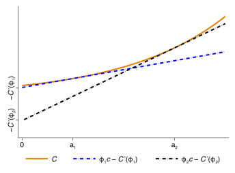
Figure 1: Legendre Transformation

Figure 1 illustrates the Legendre transformation through the tangent lines of the convex resource cost function of providing consumption utility in (31). The dashed lines are tangent lines of the resource cost function with slope $\varphi$. The corresponding value of the Legendre transform is the negative of the $y$-intercept for this tangent line, $-\mathcal{C}^{*}(\varphi)$.

A convex function exceeds all tangent lines. For any consumption utility $c$, and for any point of tangency $a$:

$$\mathcal{C}(c)\geq\mathcal{C}(a)+(c-a)\mathcal{C}^{\prime}(a)=\varphi c-\mathcal{C}^{*}(\varphi),$$ (31)

where the equality follows by parameterizing the tangent lines with their slope $\varphi:=\mathcal{C}^{\prime}(a)$ and by letting $\mathcal{C}^{*}(\varphi):=-\mathcal{C}(a)+a\mathcal{C}^{\prime}(a)$ for $a={\mathcal{C}^{\prime}}^{-1}(\varphi)$. The function $\mathcal{C}^{*}$ is called is the Legendre transformation for the resource cost of providing consumption utility $\mathcal{C}$. Since a convex function exceeds all of its tangent lines, and since the function value equals the value of the tangent line at the point of tangency:

$$\mathcal{C}(c)=\max_{\varphi\geq 0}\;\varphi c-\mathcal{C}^{*}(\varphi).$$ (32)

The Legendre transformation converts the convex resource cost of providing consumption utility on the left side of (32) into a family of linear constraints on the right. The family of linear constraints is parameterized by the slopes of the tangent lines to the cost function. Since the resource cost increases with consumption utility, the slopes of the tangent lines are positive, or $\varphi\geq 0$.

Figure 1 shows the Legendre transformation through the tangent lines of the convex resource cost function of providing consumption utility in (31). For example, the blue dashed is the tangent line of the resource cost function at point $a_{1}$, which has a slope $\varphi_{1}$. The value of the Legendre transform corresponding to the slope $\varphi_{1}$ is the negative of the $y$-intercept for this tangent line, as denoted by $-\mathcal{C}^{*}(\varphi_{1})$.

The previous steps hold for any convex function, allowing us to apply the same argument to transform the resource cost of providing work disutility into a family of linear constraints:

$$\mathcal{X}_{s}(x_{s})=\max_{\psi_{s}\leq 0}\;\psi_{s}x_{s}-\mathcal{X}_{s}^{*}(\psi_{s}),$$ (33)

for each skill $s\in\mathcal{S}$. An increase in production disutility increases production and therefore lowers resource costs. The resource cost of production disutility is decreasing, implying negative slopes of the tangent lines, or $\psi_{s}\leq 0$.

To summarize, the transformed planning problem is to minimize the resource cost of providing utilitarian welfare $\mathcal{U}$:

$$\int\Big{(}\max_{\varphi(p)}\big{(}\varphi(p)c(p)-\mathcal{C}^{*}(\varphi(p))\big{)}+z(p)\sum_{s}\max_{\psi_{s}(p)}\big{(}\psi_{s}(p)x_{s}(p)-\mathcal{X}_{s}^{*}(\psi_{s}(p))\big{)}\Big{)}\pi(p)\text{d}p$$ (34)

subject to incentive constraints (13) for all workers $(p,q)\in P\times P$, linear outside option constraints (14) for all workers $p\in P$, and the linear promise keeping condition (15). In Section A.8, we show this planning problem is equivalent to maximizing utilitarian welfare subject to the resource constraint, the incentive constraints, and the outside option constraints. In Section A.9 we show how to derive the stochastic dominance condition and the general ABC formula directly from the transformed planning problem.

Numerical Approach. The only nonlinear part of the optimization problem that remains to be linearized is the objective:

$$\min\int\left(\mathcal{C}(c(p))+z(p)\big{(}\mathcal{X}_{c}(x_{c}(p))+\mathcal{X}_{m}(x_{m}(p))\big{)}\right)\pi(p)\text{d}p.$$ (35)

To illustrate our approach, we focus on the linearization of the convex resource cost function for consumption utility $\mathcal{C}$, and we suppose that boundaries for the optimal solution are known a priori, or $\underline{c}(p)\leq c(p)\leq\bar{c}(p)$ and $\underline{x}_{s}(p)\leq x_{s}(p)\leq\bar{x}_{s}(p)$.

The idea is to approximate the convex cost for consumption utility $\mathcal{C}$ from below with the tangent lines on the bounded interval. For each worker $p$, it follows from the definition of the Legendre transform (32) that $\mathcal{C}(c(p))=\max\limits_{\varphi}\varphi c(p)-\mathcal{C}^{*}(\varphi)$. We numerically replace this continuous set of tangent slopes $\varphi$ in the definition of the Legendre transform with a finite set of tangent lines. Specifically, we consider a list of slopes $\{\varphi_{i}(p)\}_{i=1}^{n}$ with corresponding tangent lines $l^{c}_{ip}(t):=\varphi_{i}(p)t-\mathcal{C}^{*}(\varphi_{i}(p))$ such that the inequality:

$$0\leq\mathcal{C}(t)-\max_{1\leq i\leq n}\;l^{c}_{ip}(t)\leq\varepsilon_{c}$$ (36)

holds for all $t$ in the bounded interval $[\underline{c}(p),\bar{c}(p)]$. Analogously, in order to linearize the resource cost of labor disutility $\mathcal{X}_{s}$, we consider a list of slopes $\{\psi^{s}_{i}(p)\}_{i=1}^{n}$ with corresponding tangent lines $l^{s}_{ip}(t):=\psi^{s}_{i}(p)t-\mathcal{X}^{*}(\psi^{s}_{i}(p))$ such that the inequality:

$$0\leq\mathcal{X}_{s}(t)-\max_{1\leq i\leq n}\;l^{s}_{ip}(t)\leq\varepsilon_{s}$$ (37)

holds for each skill $s\in\mathcal{S}$ and for all $t$ in the interval $[\underline{x}_{s}(p),\bar{x}_{s}(p)]$.

As a key step, we next introduce independent auxiliary variables $r(p)$ for each worker $p$ satisfying the following set of linear inequalities for all $i$:

$$r(p)\geq\varphi_{i}(p)c(p)-\mathcal{C}^{*}(\varphi_{i}(p)).$$ (38)

It follows from the discussion above that $r(p)\gtrsim\mathcal{C}(c(p))$ for each worker $p$. For the resource cost of disutility from working, we similarly define independent auxiliary variables $r_{s}(p)$ satisfying the linear inequalities for all $i$:

$$r_{s}(p)\geq\psi^{s}_{i}(p)x_{s}(p)-\mathcal{X}^{*}(\psi^{s}_{i}(p)).$$ (39)

We substitute the auxiliary variables $r(p)$ and $r_{s}(p)$ for $\mathcal{C}(c(p))$ and $\mathcal{X}_{s}(x_{s}(p))$ into our nonlinear objective to define the approximate planner problem. The approximate planner problem chooses $(c,x_{s},r,r_{s})$ to solve:

$$\min\int\left(r(p)+z(p)\big{(}r_{c}(p)+r_{m}(p)\big{)}\right)\text{d}\pi,$$ (40)

subject to the incentive constraints (13), the outside option constraints (14), the promise keeping constraint (15), constraints on the auxiliary variables (38) and (39), and the approximation bounds for consumption utility $\underline{c}(p)\leq c(p)\leq\bar{c}(p)$ and task outputs $\underline{x}_{s}(p)\leq x_{s}(p)\leq\bar{x}_{s}(p)$.

In Appendix A.10 we prove the theoretical accuracy of the approximate planner problem and describe the algorithm that we use to characterize the numerical solution.

5 Positive Economy

In this section, we describe and characterize an equilibrium in a positive model of workers with multidimensional skills sorting with heterogeneous firms.

Firm. Every firm $z$ takes wage schedule $w$ as given and chooses two workers to solve:

$$\Omega(z)=\max_{x_{1},x_{2}}\;y(x_{1},x_{2},z)-w(x_{1})-w(x_{2}).$$ (41)

We define the surplus function $S$ as output minus payments to the workers and the firm:

$$S(x_{1},x_{2},z):=y(x_{1},x_{2},z)-w(x_{1})-w(x_{2})-\Omega(z).$$ (42)

The output of a firm cannot exceed payments to its workers and owner, that is, $S(x_{1},x_{2},z)\leq 0$ for any triplet $(x_{1},x_{2},z)$.

Worker. Every worker takes the wage schedule $w$ as given and chooses their cognitive and manual task inputs $x$ to solve:

$$\max_{x_{c},x_{m}}\;u(c)-v\Big{(}\frac{x_{c}}{\alpha_{c}}\Big{)}-v\Big{(}\frac{x_{m}}{\alpha_{m}}\Big{)}$$ (43)

subject to the budget constraint $c=(1-\tau)w(x)$, where $w(x)=w(x_{c},x_{m})$ is the wage as a function of both cognitive and manual inputs, and the disutility from work is given by (2). The government taxes earnings at a linear rate $\tau$ to finance public expenditures $G$ that are not valued (or valued separately) by workers.

Resources. The resource constraint is given by:

$$\int y(x_{1},x_{2},z)\text{d}\gamma(x_{1},x_{2},z)=\int c(\alpha)\text{d}\Phi(\alpha)+\int\Omega(z)\text{d}F_{z}(z)+G.$$ (44)

Total production, $\int y(x_{1},x_{2},z)\text{d}\gamma(x_{1},x_{2},z)$, equals output distributed to workers, $\int c(\alpha)\text{d}\Phi(\alpha)$, to firms $\int\Omega(z)\text{d}F_{z}(z)$, and to public expenditures $G$.

Equilibrium. A competitive equilibrium is a wage schedule $w$, a worker input distribution $F_{x}$, a feasible assignment $\gamma$, and an allocation $\{(c(\alpha),x_{c}(\alpha),x_{m}(\alpha))\}$ such that firms solve their profit maximization problem (41), workers solve the worker’s problem (43), the government budget constraint is satisfied $G=\tau\int w(x)\text{d}\Phi(\alpha)$, and the resource constraint (44) is satisfied.

5.1 Characterizing Equilibrium

To characterize an equilibrium, we relate our positive economy to optimal transport problems (Villani, 2003; Galichon, 2018).

Primal Problem. The primal problem is to choose an assignment to maximize production:

$$\max_{\gamma\in\Gamma}\;\int y(x_{1},x_{2},z)\text{d}\gamma.$$ (45)

The choice of the assignment function is restricted by the feasibility constraint, $\gamma\in\Gamma(F_{x},F_{x},F_{z})$. $\Gamma$ denotes the set of probability measures on the product space $X\times X\times Z$ such that the marginal distributions of $\gamma$ onto $X$ and $Z$ are $F_{x}$ and $F_{z}$ respectively.

Dual Problem. The dual transport problem is to choose functions $w$ and $\Omega$ that solve:

$$\min\;\int w(x_{1})\text{d}F_{x}+\int w(x_{2})\text{d}F_{x}+\int\Omega(z)\text{d}F_{z},$$ (46)

subject to the constraint that the surplus function is weakly negative for any triplet $(x_{1},x_{2},z)\in X\times X\times Z$, that is, $S(x_{1},x_{2},z)\leq 0$.

We connect the primal problem and the dual problem to equilibrium in Lemma 3.

Lemma 3.

The equilibrium assignment $\gamma$ solves the primal problem (45), equilibrium wages $w$ and firm value $\Omega$ solve the dual problem (46).

The proof is in Appendix A.11. We use Lemma 3 to characterize the equilibrium assignment and equilibrium wages. We solve the primal problem (45) to characterize the equilibrium assignment function and the dual problem (46) to characterize wages $w$ and firm value $\Omega$.

Equilibrium Characterization. We observe that solving for the equilibrium assignment in the positive economy follows the same steps as solving for the planner assignment in Section 3.1. It thus follows from Proposition 1 that the equilibrium features self-matching between workers and coworkers, and positive sorting between team quality and firm project values.

To characterize wages and firm values, we use Lemma 3 and solve the dual transportation problem. Since the surplus is negative for any triplet in equilibrium, $S(x_{1},x_{2},z)\leq 0$, and since the aggregate resource constraint (44), the government budget constraint and the household budget constraints hold in equilibrium, the surplus equals zero almost everywhere with respect to the equilibrium assignment, so $w(x_{1})+w(x_{2})+\Omega(z)=y(x_{1},x_{2},z)$. Firm output is distributed to its owner and to its workers. We use this condition to establish properties of the firm value function and the wage schedule.

We first note that wages are only a function of effective worker skills $X=x^{2}_{c}+x^{2}_{m}$, and we define $h(X)$, the firm’s total wage bill, as $h(X):=2w(x)$. By applying standard arguments from optimal transport, wages are convex in effective skill $X$, so small differences in effective worker skill translate into increasingly large differences in worker earnings, and the firm value function is the Legendre transform of the wage bill, $\Omega=h^{*}$. As a result, $h(X)+h^{*}(z)=zX$. The derivation of these properties is presented in Section A.13.

In our quantitative analysis, we infer the distribution of project values $F_{z}$ using earnings data. The key is to show that there exists a firm project $z$ such that $h(X)+h^{*}(z)=zX$ for any pairing $(z,X)$. When the wage bill $h$ is continuously differentiable the derived fact that $h(X)+h^{*}(z)=zX$ implies $z=h^{\prime}(X)$. That is, the derivative of the firm’s wage bill is equal to its project value. Given some increasing and convex wage bill $h$, and effective skills $X$, this condition identifies increasing values for firm productivity $z$.

We apply this logic to the parametric continuously differentiable function $h(X)=X^{\eta}+2\zeta$ where $\eta\geq 1$ governs the convexity of the wage bill and $\zeta$ captures the lowest wage per worker. Using the derived fact that $z=h^{\prime}(X)$, we can relate the distribution of firm projects $z$ to the convexity parameter $\eta$ of the wage bill. In the limit where $\eta$ is equal to 1, there is no dispersion in firm productivity. We formalize this in Lemma 4.

Lemma 4.

For some firm distribution $F_{z}$ there exists an equilibrium with ($i$) a self-matched assignment, and ($ii$) a wage function:

$$w(x)=\frac{1}{2}\big{(}x^{2}_{c}+x^{2}_{m}\big{)}^{\eta}+\zeta.$$ (47)

The proof is in Appendix A.14. The idea is to show there is a firm distribution $F_{z}$ such that given wage schedule (47), workers and firms both optimize in a self-matching equilibrium. Given the firm technology (4) and the wage equation (47), firm profits are decreasing in the difference between their workers’ skills. To minimize output losses, firms thus hire pairs of identical coworkers. Given wage equation (47), the worker problem has a unique solution, implying that the distribution of worker inputs $F_{x}$ is uniquely determined by the worker problem. Finally, we map the firm distribution that induces (47) as an equilibrium wage equation using $z=h^{\prime}(X)$. We next use this equilibrium construction to establish pointwise identification of the worker skill distribution for all U.S. workers.

6 Quantitative Analysis

In this section we infer the distribution of cognitive and manual talents $\Phi$. The estimation of the underlying distributions of skills, a central input for the calculation of the optimal tax formula, generalizes the derivation of the unidimensional skills in Saez (2001) to a labor market model with multidimensional skills, coworker and firm effects. We also calibrate the parameter $\rho$ that governs the curvature of disutility with respect to effort.

6.1 Data Sources

We use data from the American Community Survey (ACS). We consider individuals between 25 and 60 years of age. The final sample from the ACS includes almost 16 million individuals between 2000 and 2019. For all our results, we use sample weights provided by the survey.

Our measure of labor income is wage and salary income before taxes over the past 12 months. This measure includes wages, salaries, commissions, cash bonuses, tips, and other money income received from an employer. We drop individuals with earnings below a threshold to focus on workers who are attached to the labor market. This minimum is equal to one-half of the federal minimum wage times 13 weeks at 40 hours per week (as in Guvenen, Ozkan, and Song (2014) and Guvenen, Karahan, Ozkan, and Song (2021)).

The ACS contains occupational information for every worker. We combine a worker with the task intensity for their occupation using O*NET task measures from Acemoglu and Autor (2011). Our cognitive measure is the average $Z$-score of their cognitive measures, and our manual measure is the average $Z$-score of their manual measures. Our resulting scores are approximately normally distributed across occupations.

For identification, we construct a measure of relative task intensity by occupation. To obtain aggregated task production levels we use a Cobb-Douglas technology to map worker subtasks into final task production similar to Kremer (1993), Acemoglu and Autor (2011) and Deming (2017):

$$q_{s}=\exp\bigg{(}\frac{1}{|\mathcal{V}|}\sum\limits_{\nu\in\mathcal{V}}\log q_{s\nu}\bigg{)}.$$ (48)

Letting $\log q_{s\nu}$ be the $Z$-score by subtask $\nu$, we obtain cognitive and manual task production levels. Since the $Z$-scores for our aggregated cognitive and manual measure are approximately normally distributed, task production levels are approximately lognormal. We now make an identification assumption that the relative task input intensity is equal to the relative task production level, $x_{m}/x_{c}=q_{m}/q_{c}$, which is hence also approximately lognormally distributed.

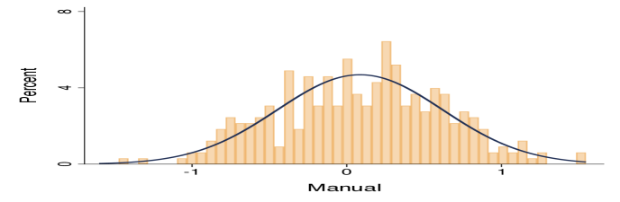
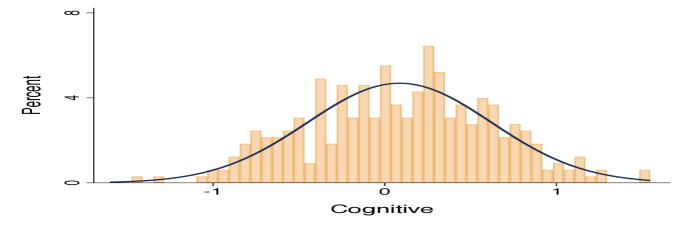
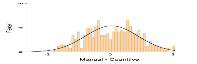
Figure 2: Task Intensity Across Occupations

Figure 2 shows the distribution of manual and cognitive task intensity across occupations in logs (left and center panel) together with the relative distribution of manual and cognitive task intensity (right panel). Each of the distributions is well-approximated by a lognormal distribution.

Figure 2 shows the distribution of manual and cognitive task intensity across occupations in logs together with the relative distribution of manual and cognitive task intensity. The first two panels show that both the distribution of cognitive task intensity and the distribution of manual task intensity can be described by a lognormal distribution. The right panel shows that the same holds for the relative manual task intensity.

Figure 3 displays the relationship between relative task intensity and average earnings across occupations. Earnings are low for occupations with high manual task intensity, such as gardeners and truck drivers, while earnings are high for occupations with high cognitive task intensity such as software developers and actuaries. Moving from the 25th percentile to the 75th percentile in relative manual task intensity decreases earnings from 62 to 35 thousand dollars.

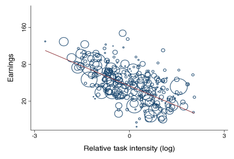
Figure 3: Earnings and Relative Task Intensity

Figure 3 show the relation between average earnings (y-axis, logarithmic scale) and relative task intensity across occupations. Average earnings are decreasing in the relative manual task intensity. Moving from the 25th percentile to the 75th percentile in relative task intensity decreases earnings from 62 to 35 thousand dollars. The size of each circle corresponds to the occupation’s employment share.

6.2 Calibration

We now calibrate the positive model. We parameterize fiscal policy and preferences, and infer the underlying multidimensional skill distribution.

The government taxes labor income to finance expenditures $G$. If pre-tax earnings are $w$, then taxes are given by $T(w)=\tau w$. After-tax earnings are thus given by $(1-\tau)w$, we set $\tau=0.3$.

Firm heterogeneity governs the convexity of the wage schedule (see Lemma 4). We set the curvature parameter for the wage schedule $\eta$ to align the added variation in log wages due to firm heterogeneity with estimates from the literature on variation in log wages due to firm effects. Using the wage equation (47), the variation in firm projects multiplies the underlying variation across workers by $\eta^{2}$. We choose $\eta=1.1$ to attribute 17 percent of the added variation in wages to firm effects. Our target of 17 percent is in line with estimates from the literature.

We next discuss the calibration of worker preferences. We use linear preferences with respect to consumption goods, $u(c)=c$, and estimate the parameter governing the curvature of the disutility function to efforts in each task $\rho$. We set $\rho$ such that a regression of log market hours on hourly wages, holding constant the marginal value of wealth, yields a coefficient of 0.55. The target value of 0.55 comes from the meta-analysis of estimates of the intensive margin Frisch elasticity from microvariation in Chetty, Guren, Manoli, and Weber (2012).

To use estimates for the Frisch elasticity of substitution of total hours with respect to hourly productivity to calibrate the curvature of the utility function with respect to effort, we derive this expression within our model. Given the specification for the disutility from work (2), the linear utility from consumption, and the worker technology (3), the worker’s problem (43) is:

$$\max\limits_{x_{c},x_{m}}\;\frac{1}{2}(1-\tau)(x_{c}^{2}+x_{m}^{2})^{\eta}-\kappa\big{(}\frac{x_{c}}{\alpha_{c}}\big{)}^{\rho}-\kappa\big{(}\frac{x_{m}}{\alpha_{m}}\big{)}^{\rho}$$ (49)

The optimality conditions to the worker’s problem for each task $s\in\mathcal{S}$ are:

$$(1-\tau)\eta\big{(}2w(x)\big{)}^{\frac{\eta-1}{\eta}}=\kappa\rho\frac{x_{s}^{\rho-2}}{\alpha^{\rho}_{s}},$$ (50)

where $w(x)=\frac{1}{2}(x^{2}_{c}+x^{2}_{m})^{\eta}+\zeta$ by wage equation (47) with $\zeta$ representing minimum earnings in our data. In words, the marginal consumption utility from supplying extra tasks equals the marginal cost of effort. Taking the ratio of these optimality conditions, this implies that the skill, effort and task intensity ratio are related by:

$$\frac{\alpha_{m}}{\alpha_{c}}=\Big{(}\frac{x_{m}}{x_{c}}\Big{)}^{\frac{\rho-2}{\rho}}=\Big{(}\frac{\ell_{m}}{\ell_{c}}\Big{)}^{\frac{\rho-2}{2}},$$ (51)

where the second equality follows from the worker task technology (3), $x_{s}=\alpha_{s}\ell_{s}$. The marginal rate of substitution between activities, $\big{(}\frac{\ell_{c}}{\ell_{m}}\big{)}^{\rho-1}$, is equal to the ratio of marginal benefits between activities, $\big{(}\frac{\alpha_{c}}{\alpha_{m}}\big{)}^{2}\frac{\ell_{c}}{\ell_{m}}$. The relative efforts are determined by the relative skills $\frac{\alpha_{c}}{\alpha_{m}}$. Workers spend more effort on tasks in which they are more talented.

Using the first-order conditions for effort, and observing that the share of total efforts on each task is constant by (51), we can express the Frisch elasticity of total hours $\ell_{c}+\ell_{m}$ as:

$$\varepsilon=\frac{\partial\log(\ell_{c}+\ell_{m})}{\partial\log z(x)}\bigg{|}_{\lambda}=\frac{\partial\log(\ell_{c}+\ell_{m})}{\partial\log(1-\tau)}\bigg{|}_{\lambda}=\frac{1}{\rho-1},$$ (52)

where $\lambda$ is the marginal value of wealth, and $z(x):=w(x)/(\ell_{c}+\ell_{m})$ is productivity per hour. We set $\rho=2.8$ so that the Frisch elasticity $\varepsilon$ is indeed $0.55$. Finally, we normalize $\kappa=\frac{1}{2\rho}$.

Skill Distribution. We now identify the skill distribution point-by-point. Using the solution to the worker’s problem (43), together with data on both total earnings and occupational relative task intensity for each worker, we exactly identify two sources of worker productivity $(\alpha_{c},\alpha_{m})$ that rationalize the data as a model outcome. This identification argument is similar to Boerma and Karabarbounis (2020, 2021) who use explicit solutions for home production models to identify productivity at home and to separately identify permanent and transitory market productivity using data on consumption, home and market hours.

Using the O*NET task measures, we have information on the relative task intensity for each occupation $\frac{x_{m}}{x_{c}}$ and, hence, we identify the relative skills $\frac{\alpha_{m}}{\alpha_{c}}$ by equation (51). To additionally determine the level of tasks, we use the wage equation (47):

$$w(x)=\frac{1}{2}\big{(}x^{2}_{c}+x^{2}_{m}\big{)}^{\eta}=\frac{x^{2\eta}_{c}}{2}\bigg{(}1+\Big{(}\frac{x_{m}}{x_{c}}\Big{)}^{2}\bigg{)}^{\eta}$$ (53)

Given the skill ratio for an individual their occupation, $\frac{x_{m}}{x_{c}}$, and an individual their wage $w(x)$, this equation uniquely determines the level of cognitive tasks $x_{c}$, and hence the level of manual tasks $x_{m}$. By the optimality condition (50), we identify both cognitive skills $\alpha_{c}$ and manual skills $\alpha_{m}$ for each worker. We illustrate the exact identification through examples and then identify the cognitive and manual skills for every worker in the ACS.

Table 1: Example

		Relative Task	Wages	Task Intensity		Task Skills
		$x_{m}/x_{c}$	$w(x)$	$x_{m}$	$x_{c}$	$\alpha_{m}^{\rho}$	$\alpha_{c}^{\rho}$
1	Baseline	1	1	1.00	1.00	0.50	0.50
2	Task intensity	3	1	1.35	0.45	0.63	0.26
3	Wages	1	4	2.00	2.00	0.87	0.87
4	Taxes $\tau=0.3$	1	1	1.00	1.00	0.71	0.71
5	Firms $\eta=1.1$	1	1	0.97	0.97	0.42	0.42

Table 1 illustrates the identification of workers’ manual and cognitive skills through five examples. We infer higher levels of manual skills with higher manual task intensity (in Row 2), higher earnings (Row 3), higher taxes (Row 4), and with less dispersion in firms’ project values (Row 5).

Examples. To provide insight into the mechanism and identification of the sources of worker heterogeneity, we consider a numerical example. We first consider an economy without taxes $\tau=0$ and without heterogeneity in firm projects, or $\eta=1$.

Suppose a worker’s occupational relative task intensity is equal to one, $\frac{x_{m}}{x_{c}}=1$, and their earnings equal mean earnings, which we normalize to one. By (53), the worker’s cognitive task intensity and the worker’s manual task intensity are equal to $1$. Using the optimality condition for task inputs (50), $\alpha_{s}^{\rho}=\frac{1}{2}$, implying the worker is equally skilled in both tasks. This worker is presented in the first row of Table 1.

Inferred manual skill increases with manual task intensity. Consider some worker with relative manual task intensity equal to three, $\frac{x_{m}}{x_{c}}=3$, and average earnings. By (53), the cognitive task intensity is $x_{c}=\frac{1}{\sqrt{5}}<1$ and hence the worker’s manual task intensity is greater with $x_{m}=\frac{3}{\sqrt{5}}>1$. Since $\alpha^{\rho}_{s}=\frac{1}{2}x_{s}^{\rho-2}$, it follows that the worker’s inferred manual skill increases with relative manual task intensity, while the worker’s cognitive skills decreases, as shown in the second row of Table 1.

Inferred skill levels increase with earnings. For a worker with a relative task intensity of one, but a high level of earnings, the relative skill intensity is one but the level of each task is greater. Consider a worker that earns four times average earnings. By (53), we identify the worker’s cognitive task intensity, and therefore the worker’s manual task intensity, to be equal to $2$. Using the worker’s optimality condition for task inputs (50), $\alpha_{s}^{\rho}=\frac{1}{2}2^{\rho-2}$, implying that the worker is equally skilled in both tasks, and almost 1.75 times as skilled as a worker in the same occupation earning average earnings. This worker is presented in the third row of Table 1.

The presence of taxes does not affect inferred task intensities $x$, but does increase the inferred skill levels $\alpha$. Since the identification of the task intensity is based on pretax earnings (53), inferred task intensities do not vary with taxes. For $\eta=1$, since the task intensity does not change with taxes, we obtain $\alpha^{\rho}_{s}=\frac{1}{2(1-\tau)}x_{s}^{\rho-2}$. When workers are taxed, the marginal benefit from completing tasks is reduced. To rationalize the same levels of cognitive and manual task intensity supplied by a worker, it must be less costly for the worker to complete tasks due to increased levels of skills, as shown in the fourth row of Table 1.

Finally, increased dispersion in firm project values decreases wage dispersion that is attributed to dispersion in task intensity. Consider the parametric introduction of dispersion in firm projects with $\eta>1$. Reorganizing the wage equation (53), $x_{c}=\left(2w(x)\right)^{\frac{1}{2\eta}}\Big{/}\sqrt{1+\left(\frac{x_{m}}{x_{c}}\right)^{2}}$, shows that higher values of $\eta$ compress the dispersion in task intensity. Further, by combining the first-order condition (50) with wage equation (53), we obtain $\alpha^{\rho}_{s}\propto w(x)^{\frac{\rho}{2\eta}-1}$. An increase in $\eta$ decreases the effective dispersion in skills. Dispersion in firm project values magnifies underlying differences in task intensity due to the positive sorting between workers and projects. Equivalently, small differences in effective worker skills generate large differences in earnings.

Table 2: Illustration of Identification

Occupation	Relative	Wages	Manual	Cognitive	Firm	SOC Code
	$\log\frac{x_{m}}{x_{c}}$	$\mathbb{E}w(x)$	$\frac{\alpha_{m}-\mathbb{E}\alpha_{m}}{\sigma_{m}}$	$\frac{\alpha_{c}-\mathbb{E}\alpha_{c}}{\sigma_{c}}$	$\frac{\alpha_{z}-\mathbb{E}\alpha_{z}}{\sigma_{z}}$
Gardeners	-1.7	125	-0.94	-2.34	-1.25	37$-$3010
Truck drivers	-1.6	140	-1.45	-1.93	-0.25	53$-$3030
Cashiers	-0.7	120	-0.47	-1.16	-1.61	41$-$2010
Police officers	-0.1	169	-0.83	-0.49	-0.84	33$-$3050
Physicians	-0.2	198	-1.79	-1.32	-3.13	29$-$1060
Software developers	-1.5	193	-1.71	-1.25	-1.46	15$-$1030
Financial managers	-1.8	198	-2.25	-1.31	-1.57	11$-$3030
Chief executives	-2.1	158	-2.39	-1.71	-2.62	11$-$1010
Actuaries	-2.7	143	-3.47	-1.63	-2.39	15$-$2010

Table 2 illustrates the identification of underlying worker skills for a number of occupations. Holding constant the relative manual skill intensity, high earnings identify high skill levels as seen by comparing the identified manual and cognitive skills of police officers and physicians. Holding constant earnings, high manual task intensity identifies high manual skills as seen by comparing the identified skills of gardeners and cashiers.

Having illustrated the identification with numerical examples, we turn to identification using earnings data. Table 2 illustrates the identification of underlying skills for representative workers in occupations listed in the first column. The second column shows the relative manual task intensity for these occupations from O*NET task measures. The third column shows average earnings of the workers by occupation in the ACS. Table 2 shows a negative relation between manual task intensity and average earnings by occupation, in line with Figure 3.

To identify manual and cognitive skills, we use equations (50), (51) and (53). First, we establish that higher earnings identify higher levels of skills, everything else equal. Holding constant the manual task intensity $x_{m}/x_{c}$, wage equation (53) shows that the level of cognitive tasks, and hence the level of manual tasks, increases by $\frac{1}{2\eta}$ percent for a one percent increase in wages. Consider an example of police officers and physicians. Since the relative task intensity for police officers and physicians is comparable, their relative skills are comparable by (51). Average earnings of physicians exceed the average earnings of police officers implying a higher level of both cognitive and manual skills for physicians. Indeed, the fourth and fifth column in Table 2 show that while both physicians and police officers’ cognitive and manual talents exceed the population average, $\alpha_{s}>\mathbb{E}\alpha_{s}$, the skills of physicians exceed the skills of police officers in both dimensions.

Second, we consider two occupations with similar wages to show that high manual task intensity identifies high manual skill all else equal. While the earnings of gardeners and cashiers are similar, gardening is more demanding in manual skills. By equation (53), this implies that the cognitive task requirements of gardeners are lower than the cognitive task requirements for cashiers. By equation (51) it follows that a gardener has more manual skills than a cashier, while the cashier has more cognitive skills than the gardener. The fourth and fifth column in Table 2 displays this pattern.

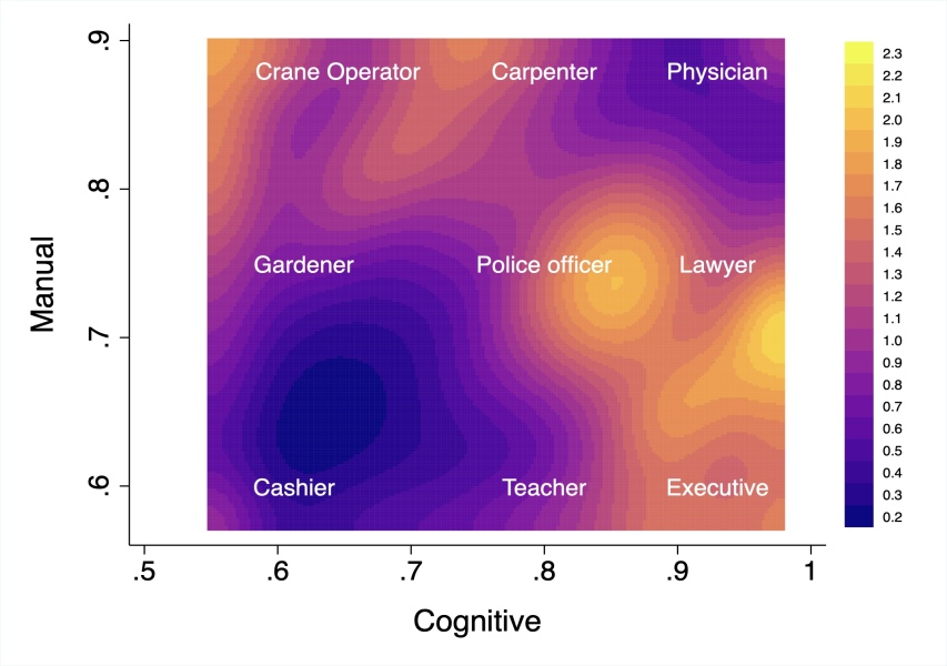
Figure 4: Inferred Skill Distribution

Figure 4 shows the inferred worker skill distribution, with bright colors indicating more mass. The panel shows the smoothed distribution of cognitive and manual skills that exactly rationalizes the data which is obtained using data on relative task intensity by occupation and worker earnings, through equations (50) to (53). The values are normalized such that one reflects a uniform distribution.

We apply the exact identification argument to data for all workers in the ACS to identify their skills. By identifying skills at the worker level, we allow for skill heterogeneity within occupations driven by earnings differences within occupation. As in the example, workers with high earnings have higher cognitive and manual skills than a worker with low earnings in the same occupation. Figure 4 shows the resulting distribution of cognitive and manual skills, after 90 percent winsorization and after smoothing the pointwise identified distribution using a kernel density estimation.

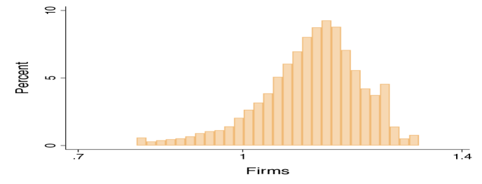
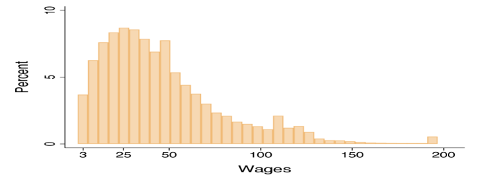
Figure 5: Firm and Wage Distribution

Figure 5 shows the histogram for the inferred firm distribution (left panel) and the model implied distribution of wages (right panel).

For illustrative purposes, it is instructive to introduce representative occupations in Figure 4. Specifically, we provide nine representative occupation within the type space. For example, cashiers are workers with both low cognitive and low manual skills, chief executives have low manual skills but high cognitive skills, while physicians have both high cognitive and high manual skills.

Finally, Figure 5 shows the inferred firm productivity distribution in the left panel and the implied wage distribution in the right panel. The left hand distribution shows that the distribution of firm projects is relatively concentrated with project values ranging from 30 percent below the mean to 20 percent above the mean (1.1). By construction, the right panel replicates the empirical distribution of wages.

7 Quantitative Results

In this section, we present the quantitative results to the planning problem using the empirically relevant model of Section 6.

7.1 Unconstrained Benchmark

To build intuition for the solution, we first present a benchmark absent any incentive constraints, outside option constraints, and firm heterogeneity. The planning problem simplifies to minimizing resource costs (11) subject to the promise keeping condition (9). By using the functional form for preferences, the promise keeping condition simplifies to:

$$\int\Big{(}c(\alpha)-\kappa\big{(}x_{c}(\alpha)\big{/}\alpha_{c}\big{)}^{\rho}-\kappa\big{(}x_{m}(\alpha)\big{/}\alpha_{m}\big{)}^{\rho}\Big{)}\text{d}\Phi\geq\mathcal{U}.$$ (54)

At an optimum, cognitive tasks are independent of workers’ routine skills, and the elasticity of cognitive tasks with respect to cognitive skills is $\frac{\rho}{\rho-2}$. Furthermore, the solution does not feature bunching. To see this, note that the following optimality condition has to be satisfied:

$$x_{s}\propto\alpha_{s}^{\frac{\rho}{\rho-2}},$$ (55)

for each skill $s\in\{c,m\}$. Owing to additive separability of tasks in both preferences and technology, the efforts on task $s$ depend only on the worker’s skills in this task. Equivalently, there is no cross-dependence between labor tasks. Since (55) describes a one-to-one relation between the worker’s skills and efforts in each task, there is no bunching at optimum. That is, within a neighborhood of worker $\alpha$, every pair of distinct workers $(\alpha^{\prime},\alpha^{\prime\prime})$ is assigned distinct allocations as $x(\alpha^{\prime})\neq x(\alpha^{\prime\prime})$.

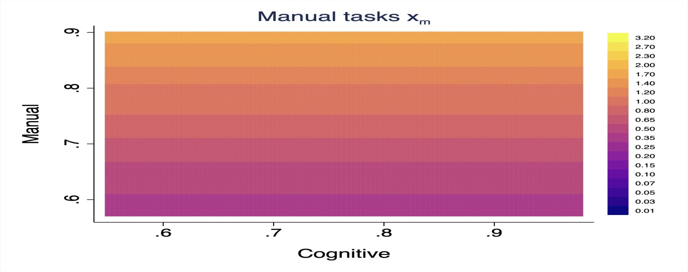
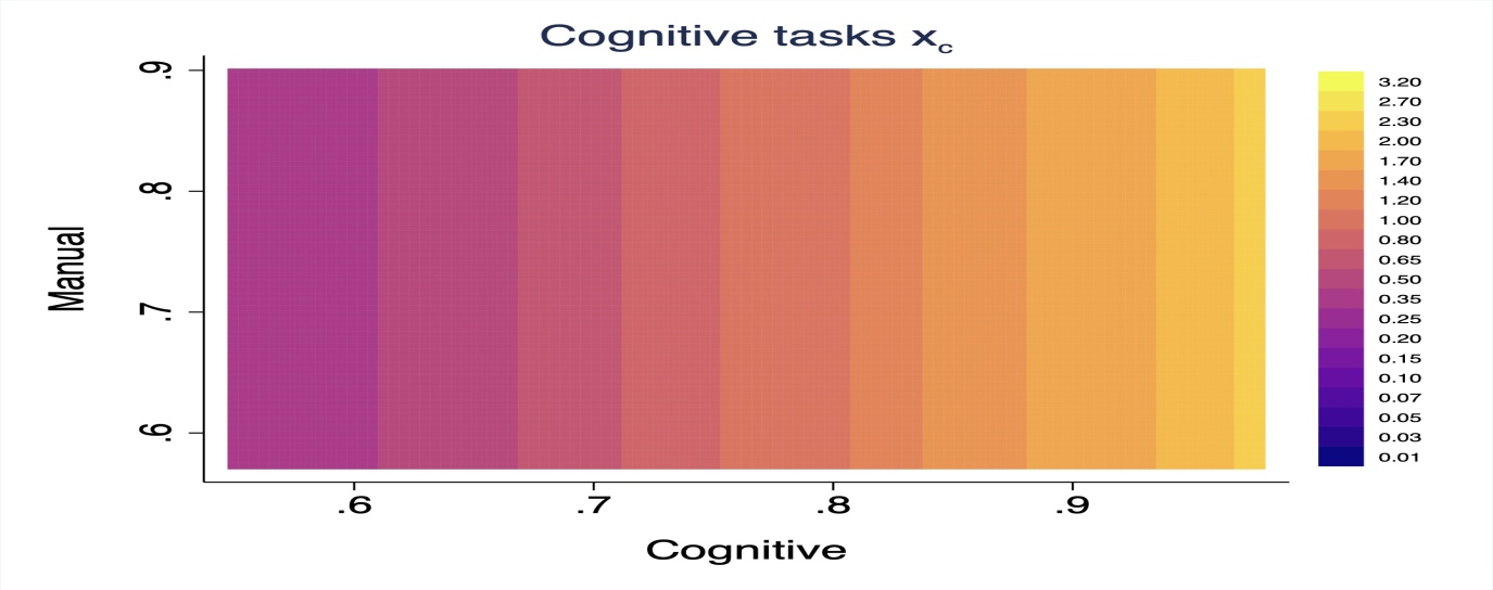
Figure 6: Benchmark Solution

Figure 6 visualizes the benchmark allocation for task intensity by worker’s cognitive and manual skills. The left panel illustrates the allocation of manual tasks $x_{m}$, the right panel shows the allocation of cognitive tasks $x_{c}$. The optimal allocation does not feature any cross-dependence between tasks. The left panel shows that manual task intensity only varies with manual skill, the right panel shows that cognitive task intensity only varies with cognitive skill.

Given the empirical description of the distribution for cognitive and manual skills in Figure 4, equation (55) describes the optimal dispersion in terms of both cognitive and manual tasks. For the skill distribution in Figure 4, the maximum to minimum skill ratio is approximately equal to 2, implying that the optimal maximum to minimum task ratio is given by $11\approx 2^{\frac{\rho}{\rho-2}}$. Introducing firm heterogeneity magnifies the optimal maximum to minimum task ratio. The increase from the dispersion in skills to the dispersion in tasks is driven by the optimal pairing of workers and coworkers. Due to the optimal self-matching of workers in both cognitive and manual tasks, production is convex in each. When a worker’s tasks increase, the direct effect is an increase in the worker’s production, while the indirect effect is an increase in the production of their coworker. Due to the indirect effect, the planner wants to increase the dispersion in each task. Absent any interactions between workers and coworkers, the production technology is linear in each task, implying an optimal elasticity of cognitive tasks with respect to cognitive skills of $\frac{\rho}{\rho-1}$. In this case, the optimal maximum to minimum ratio is only equal to $3\approx 2^{\frac{\rho}{\rho-1}}$.

Figure 6 visualizes the benchmark allocation of task intensity by worker’s cognitive and manual skills. The left panel shows the allocation of manual tasks, the right panel shows the allocation of cognitive tasks. Since (55) rules out any cross-dependence between tasks, the optimal allocation is captured by parallel horizontal and vertical lines, respectively. The left panel shows that manual task intensity only varies with manual skill, the right panel shows that cognitive task intensity only varies with cognitive skill.

7.2 Optimal Solution

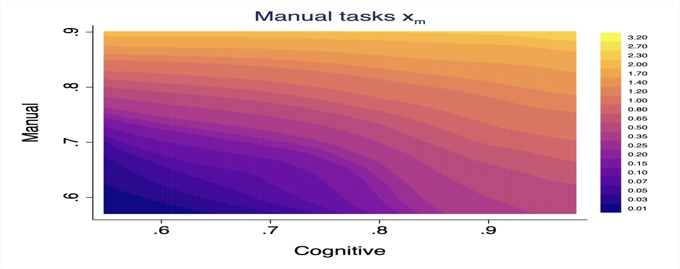
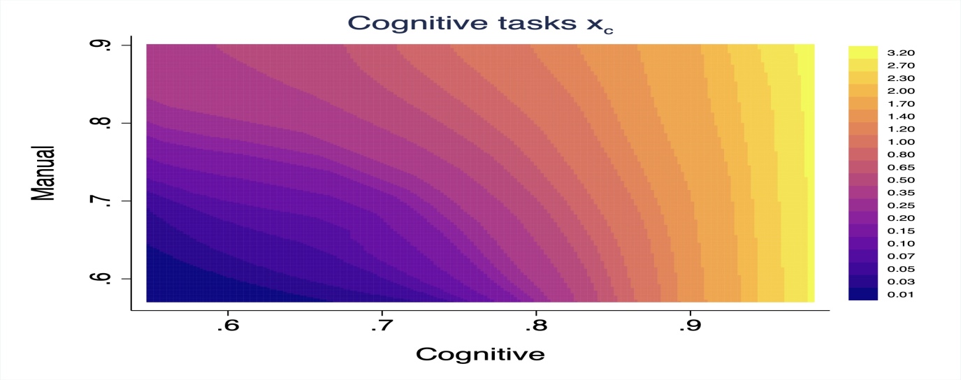
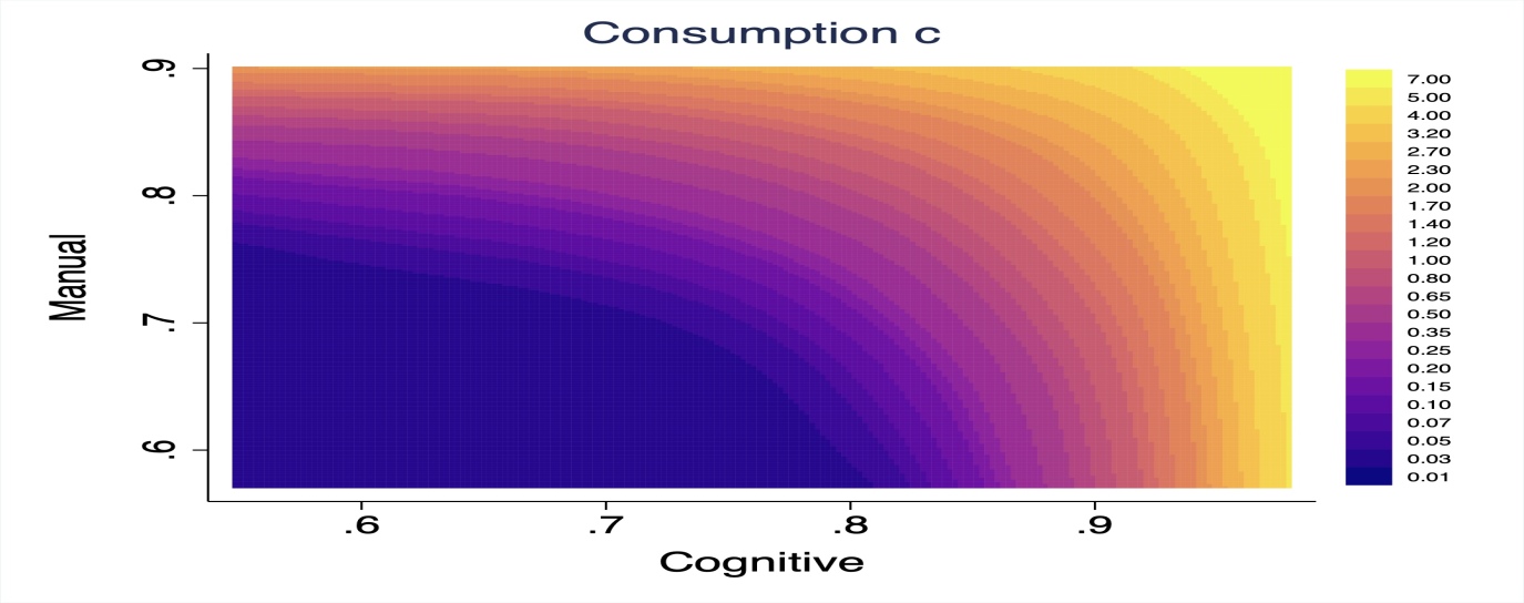
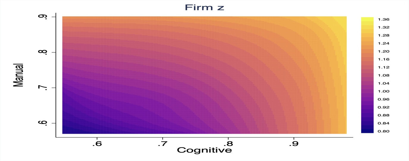
Figure 7: Solution

Figure 7 visualizes the planner solution by worker’s cognitive and manual skills. The top row shows the allocation of manual and cognitive tasks, the bottom row shows the allocation of consumption and the assignment of workers to firms. The optimal allocation features cross-dependence between tasks. For example, in contrast to the benchmark, optimal cognitive task intensity depends positively on a worker’s routine skills.

Figure 7 shows the solution to the planner problem. The top row shows the allocation of manual and cognitive tasks, the bottom row shows the allocation of consumption and the assignment of workers to firms. In contrast to the benchmark, optimal task intensity in one skill depends positively on a worker’s other skills. Consider the manual task allocation in the top left panel. Similar to the benchmark solution, the manual task intensity increases with a worker’s manual skills holding constant their cognitive skills. In contrast to the benchmark solution, the manual task intensity also increases with workers’ cognitive skills. That is, workers with the same manual ability but with a higher cognitive ability have a higher level of the manual task. Moreover, this codependence between cognitive skills and manual tasks intensifies at low levels of cognitive skills. This can be seen by the contour lines being almost negative 45 degree lines at the lower level of manual abilities, while being almost flat at the high level of manual abilities as in the case without incentive problems. The same pattern is true for the cognitive tasks.

To illustrate, consider an example of a cashier (low manual/low cognitive), an executive (low manual/high cognitive), a crane operator (high manual/low cognitive), and a physician (high manual/high cognitive). Differences between cashiers and executives as well as differences between crane operators and physicians are exclusively driven by differences in cognitive skill. Under the benchmark without the incentive constraints, a cashier and an executive conduct identical levels of manual tasks, being identical in terms of their manual skills. In the optimal solution, however, the executive who has high cognitive skills conducts a higher level of manual tasks. In contrast, consider a crane operator and a physician who have high manual skills but the crane operator has low cognitive skills. Under both the benchmark allocation and the full solution, a crane operator and a physician conduct almost identical levels of manual tasks and are thus undistorted in this dimension. The top left panel of Figure 7 shows that the solution features similar positive codependence between manual tasks and cognitive skills at all other levels of cognitive skills.

The bottom left panel shows the solution for consumption. Consumption increases with skills. Consumption of workers with top cognitive skills exceeds consumption of workers with top manual skills due to higher absolute levels of skill. The bottom right panel shows the assignment of workers to firms. Given the output of cognitive and manual tasks, the planner assigns workers with greatest effective skills $X=x^{2}_{c}+x^{2}_{m}$ to projects of greater value following Proposition 1. For example, a physician works on a more valuable project than a cashier as in the positive economy. Since the range of the cognitive skills is higher than the range of the manual skills, the high value projects are assigned towards workers with greater cognitive skills.

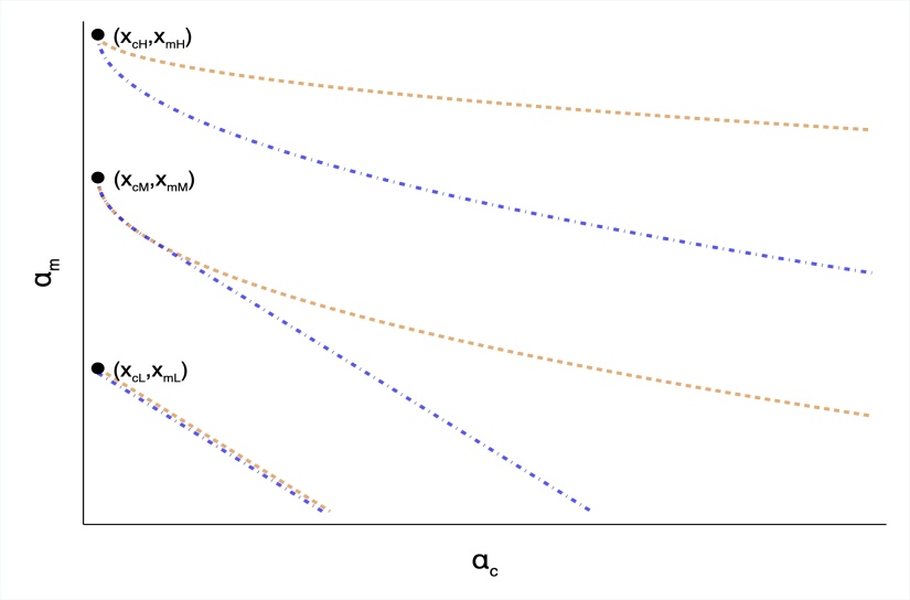
Figure 8: Illustration of Bunching

Figure 8 visualizes the procedure to determine bunching using hypothetical isocurves. The orange lines represent isocurves for different cognitive task levels, while the blue lines represent isocurves for different manual task levels. Worker $\alpha$ is bunched with worker $\alpha^{\prime}\neq\alpha$ if the isocurves for $x(\alpha)$ intersect $\alpha^{\prime}$. The isocurves for $x(\alpha_{M})$, which correspond to gardeners’ tasks, intersect for relatively high levels of manual skill and for relatively low levels of cognitive skill $\alpha_{c}$. Gardeners bunch with workers whose comparative advantage also lies in manual work.

Bunching. We now describe the nature of bunching in the optimal solution. Bunching means that different workers are assigned identical labor supply allocations and, therefore, are also assigned the same consumption allocation (see Section 3.4).

When different worker types bunch, they are assigned identical task levels. A worker $\alpha$ is bunched if there are any other workers who are assigned the same task levels $x(\alpha)$. Visually, we draw the isocurves corresponding to both $x_{c}(\alpha)$ and $x_{m}(\alpha)$ displayed on Figure 7 in the worker space $\alpha$ and assess whether the isocurves intersect for any other worker $\alpha^{\prime}$. If there exists a worker $\alpha^{\prime}\neq\alpha$ such that the isocurves intersect, then workers $\alpha$ and $\alpha^{\prime}$ are bunched.

Figure 8 gives an example of the procedure to determine optimal bunching using isocurves. The orange lines represent isocurves for different cognitive task levels, while the blue lines represent isocurves for different manual task levels. The dots indicate three hypothetical allocations. First, consider the isocurves corresponding to the allocation of crane operators in the top left corner. The orange isocurve represents workers with other combinations of skills $(\alpha_{c},\alpha_{m})$ who produce the same cognitive tasks $x_{cH}$ as the crane operator. The blue isocurve represents workers with other combinations of skills $(\alpha_{c},\alpha_{m})$ who produce the same manual tasks $x_{mH}$ as the crane operator. The lines intersect only at one point $-$ the skills of the crane operator at the top left corner. That is, no other worker type $(\alpha_{c},\alpha_{m})$ receives the same task allocation $(x_{cH},x_{mH})$ that is assigned to the crane operator. Next, consider the isocurves corresponding to the allocation of a gardener in the middle of Figure 8. The orange isocurve (workers producing the same cognitive tasks $x_{cM}$ as the gardener) overlaps with the blue isocurve (workers producing the same manual tasks $x_{mM}$ as the gardener) for high levels of manual skill $\alpha_{m}$ and for relatively low levels of cognitive skill $\alpha_{c}$. This range of workers $(\alpha_{c},\alpha_{m})$ produces the same cognitive and manual tasks $(x_{cM},x_{mM})$ as the gardener. This indicates that gardeners bunch with workers whose comparative advantage also lies in manual work. This is the targeted bunching region. Note that for the higher skills the planner separates the workers. Finally, consider the bottom-left allocation corresponding to cashiers. In this case, the orange and blue isolines for cognitive and manual tasks overlap throughout the type space. All workers with skills $(\alpha_{c},\alpha_{m})$ on that line produce the same cognitive and manual tasks $(x_{cL},x_{mL})$ as the cashier, despite their differences in skills. This is the region of blunt bunching where the planner does not distinguish the skills of the workers when allocating tasks.

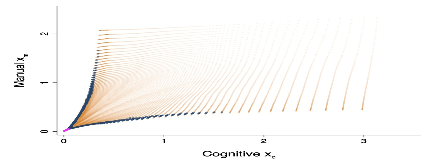
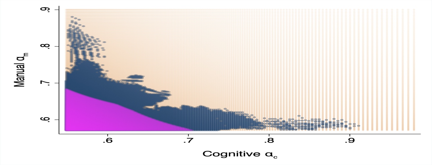
Figure 9: Optimal Bunching

Figure 9 shows bunching at the solution. The left panel demonstrates bunching in the allocation space by displaying combinations of optimal cognitive and manual tasks $(x_{c},x_{m})$. An allocation is marked in pink or in blue if the allocation is assigned to more than one worker, while the allocation is marked orange if the allocation is assigned to one worker. The right panel displays bunching in the worker type space $(\alpha_{c},\alpha_{m})$. In this figure, a worker type is marked in pink or in blue if the worker’s task allocation is also assigned to another worker. The pink area indicates the blunt bunching region while the blue area indicates the targeted bunching region.

Figure 9 shows bunching at the optimal solution and presents two complementary views of the issue. The left panel displays bunching through the allocation of labor tasks. That is, we display the combinations of the cognitive and manual tasks $(x_{c},x_{m})$ that are optimal. An allocation is marked in pink or in blue if the allocation is assigned to more than one worker, while the allocation is marked orange if the allocation is assigned to one worker. There are two main regions of bunching in this picture. The first region is that of the blunt bunching and is given by the pink line segment at the very bottom of both of the cognitive and manual tasks. The second region is that of the targeted bunching and is represented by two blue line segments at the borders of the task trapezoid. That is, targeted bunching happens when the task intensity is low for only one task. The lower (flat) blue line segment represents the low manual tasks, and the upper (vertical) line segment represents the low cognitive tasks. Note that even for these borders, when the task intensity becomes sufficiently high, the allocations are no longer bunched – that is, the blue line turns into the orange line on the edges of the trapezoid.

To see which workers are bunched, the right panel shows bunched workers in the type space $(\alpha_{c},\alpha_{m})$. In this figure, a worker type is marked in blue if the worker’s task allocation is also assigned to another worker. This panel shows that bunched workers have low cognitive or low manual skills (or both). Workers with high manual or high cognitive skills may be bunched when their skill set is asymmetric. Workers with high cognitive skills bunch when their manual skills are low, and vice versa. To quantify the extent of bunched workers in the economy, we overlay the right panel with the worker type distribution of Figure 4. At the optimum, 9.8 percent of the workers is bunched. The blunt bunching region comprises 30 percent of bunched workers. The targeted bunching region comprises 70 percent of bunched workers.

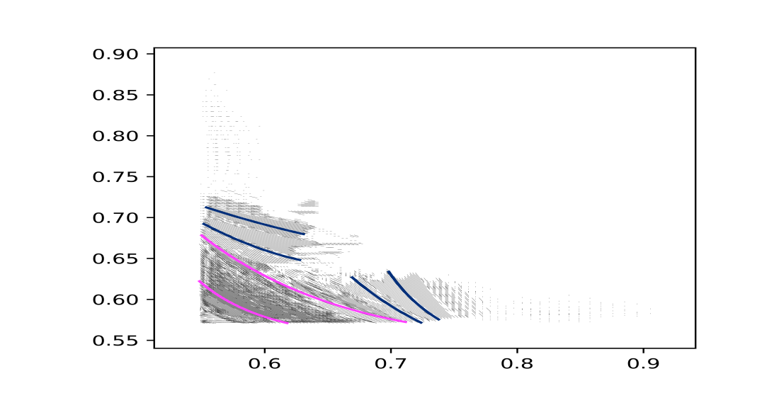
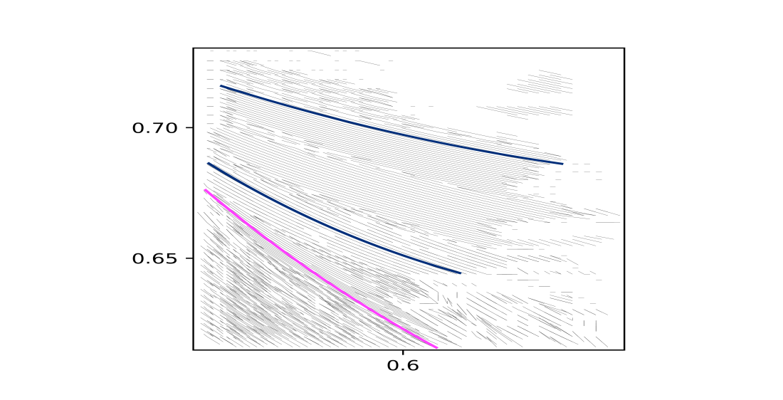
Figure 10: Bunching Patterns

Figure 10 shows with whom workers bunch by connecting workers with a line in the worker type space if their allocations are bunched. Workers exclusively bunch with workers that are better in one skill dimension, but worse in another as represented by downward-sloping lines. Pink lines indicate the blunt bunching region, while blue lines indicate bunching patterns in the targeted bunching region. Under blunt bunching, workers on the vertical boundary bunch with workers on the horizontal boundary, unlike under targeted bunching. The right-hand panel zooms in to distinguish the blunt bunching region from the targeted bunching region.

Workers bunch with other workers both near and afar. While Figure 9 shows at what allocations workers are bunched and which workers are bunched, it does not show with whom workers bunch. These bunching relations are shown in Figure 10. This figure connects two workers with a line in the type space if their allocation is marked as bunched.

Workers do not bunch with workers over whom they have an absolute advantage or who have an absolute advantage over them. Workers exclusively bunch with workers that are better in one skill dimension, but worse in another. In Figure 9 this is evident since all connections are represented by downward-sloping lines. Gardeners with somewhat better cognitive skills, but somewhat lower manual skills are bunched with colleagues with less cognitive skills, and higher manual labor skills. Despite their slight difference in skill composition, the planner assigns both identical tasks.

Within our bunching regions we distinguish two distinct patterns. In the lower triangle, which we indicate by pink lines, the planner bunches together cognitive and manual tasks for all workers, ranging from those with relatively high manual skills to those with relatively high cognitive skills. Workers with the same effective skill index produce the same cognitive and manual tasks. Work is not tailored towards workers’ specific skills, but rather to an overall level of their skills. In the blunt region, the planner deters misreporting by assigning identical allocations to different workers. Deviations are trivially deterred among these workers but at great efficiency costs.

The planner also bunches workers in the targeted bunching regions, but in a less rudimentary fashion because the efficiency cost of bunching increases with workers’ skills. The planner separately bunches together cognitive and manual tasks for workers that are relatively skilled in manual tasks and similarly bunches together the cognitive and manual tasks for workers that are relatively skilled in cognitive tasks. Unlike in the lower triangle, however, workers that are relatively skilled in cognitive labor no longer bunch with workers that are skilled in manual labor.

In the regions without bunching, the planner distorts allocations to deter deviations by workers to allocations they find desirable similar to the canonical unidimensional case. This is incentive provision through distinct distorted allocations.

Taxation. Having analyzed the planner allocation, we study the implications for optimal taxes. Specifically, we study the labor wedge (18) for cognitive and manual tasks. Using linear preferences for consumption, the labor wedge (18) can also be expressed as:

$$1-\tau_{s}=\frac{1}{2}\frac{x_{s}(\alpha)^{\rho-2}}{z(\alpha)\alpha_{s}^{\rho}}\qquad\implies\qquad\log(1-\tau_{s})\propto-\log z+(\rho-2)\log x_{s}-\rho\log\alpha_{s}.$$ (56)

The labor wedge is determined by the optimal assignment through $\log z$, by the allocation of tasks through $(\rho-2)\log x_{s}$, and by worker skills through $\rho\log\alpha_{s}$. Workers at better firms optimally face a higher labor wedge. If the planner reduces tasks, the labor wedge increases. Keeping allocations constant, the labor wedge increases when workers are more skilled.

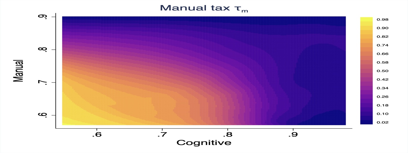
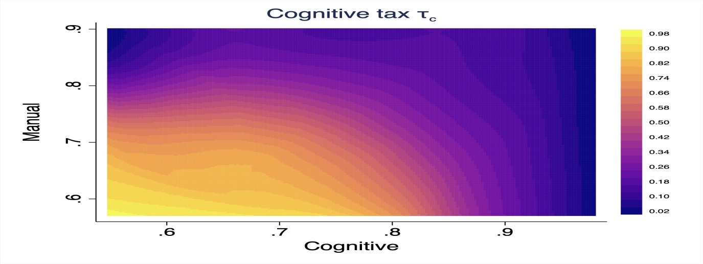
Figure 11: Tax Wedges

Figure 11 visualizes the tax wedges for the planner solution. The left panel displays the manual tax wedge, the right panel displays the cognitive tax wedge.

The optimal tax wedges are presented in Figure 11. First, the respective wedge is zero for the worker with the highest respective skill. Consider the graph for the manual tax in the left panel. Workers with the highest manual skill are those represented by the top horizontal boundary of the graph. The manual tax on them is zero. Note that for the workers with the top cognitive skill, who are represented as the right vertical boundary, the manual tax is not zero. The manual tax on the best crane operator (highest manual and low cognitive) and a physician (highest manual and high cognitive) is zero while it is positive on the best executive (low manual and highest cognitive).

The reverse is true for the cognitive tax, which is displayed in the right panel of Figure 11. The cognitive tax on the workers with the highest cognitive skill is zero. For workers with the top manual skill the cognitive tax is not zero. The cognitive tax on top executives (low manual and highest cognitive) and a physician (highest manual and high cognitive) are zero while it is positive on the best crane operator (highest manual and low cognitive).

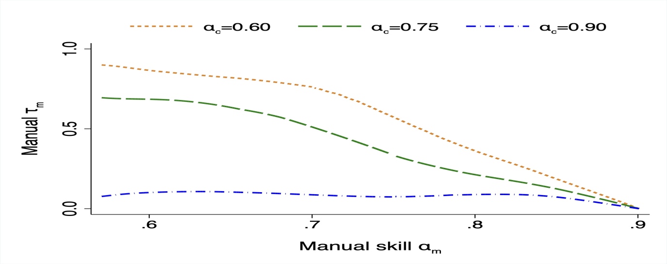
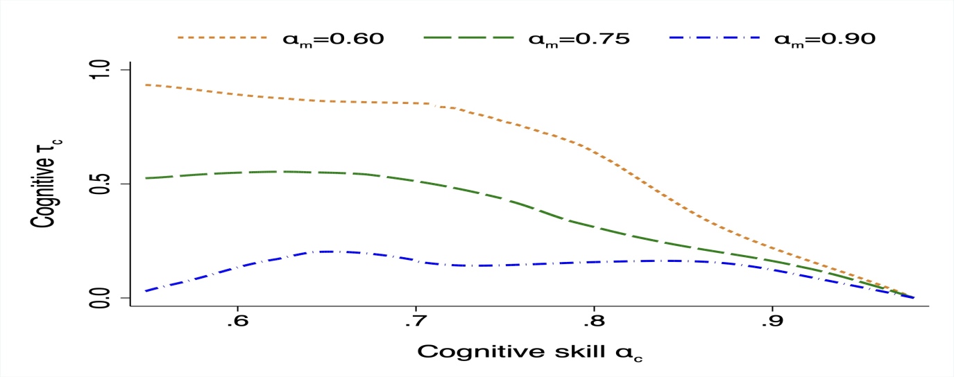
Figure 12: Manual and Cognitive Tax Wedge

Figure 12 describes how the tax wedges vary with the level of worker skill. Figure 12 displays the manual wedge in the left panel, and the cognitive tax wedge in the right panel, for three groups of workers separated by their cognitive and manual skills, respectively.

Second, we describe how taxes change with the level of the skill. Figure 12 plots the manual (on the left) and cognitive taxes (on the right) for three groups of workers separated by their skills that correspond to the heatmap in Figure 11. Consider top manual workers. Those are physicians (high cognitive), carpenters (medium cognitive), and crane operators (low cognitive). These workers are located in the top horizontal strip of Figure 11 and represented by the blue dash-dotted line in the right panel of Figure 12. These workers are not in bunched regions, and the cognitive tax on them is generally low.

Consider medium manual workers. Those are lawyers (high cognitive), police officers (medium cognitive), and gardeners (low cognitive). These workers are located in the middle horizontal strip of Figure 11 and are represented by the green dashed line in the right panel of Figure 12. The cognitive tax on them is higher and less hump-shaped. Three forces give this shape stemming from equation (56) $-$ the assignment to the heterogeneous firms, the task allocation, and the worker skill. The assignment is monotonic: lawyers are assigned to better firms than police officers and gardeners. This force gives a higher labor wedge on lawyers compared to the gardeners. Conversely, the task allocation increases with skills leading to a reduction in labor wedges. Finally, the labor wedge increases in worker skills. The low cognitive skill workers (gardeners) face a higher cognitive labor wedge than the highest cognitive skill workers (lawyers) which is hence driven by the low amounts of cognitive tasks they conduct. The high level of tax distortion on gardeners is also driven by the fact that they are bunched while lawyers and police officers are not bunched. Gardeners are located in the targeted bunching region. Their comparative advantage is in their manual skill and they are more separated along the manual dimension but bunched more in the cognitive dimension.

Consider low manual workers. Those are executives (high cognitive), teachers (medium cognitive), and cashiers (low cognitive). These workers are located in the lowest horizontal strip of Figure 11 and are represented by the orange dotted line in the right panel of Figure 12. The cognitive tax on them is higher than on medium manual workers. The cognitive tax is generally decreasing in skill with executives facing a lower marginal tax rate than cashiers. The high level of distortions on cashiers and teachers is also driven by the fact that they are both bunched. The teachers are in the targeted bunching region – they have comparative advantage in their cognitive skills and are more separated along the cognitive dimension but bunched more in the manual dimension. The cashiers are in the blunt bunching region. They are bunched in both the manual and the cognitive dimensions and this leads to their allocation being heavily distorted compared to the benchmark.

In the left panel of of Figure 12 we repeat the tax analysis for the manual tax skill wedge. Finally, in Appendix B we analyze robustness of our results with respect to firm heterogeneity.

8 Conclusion

We advance the understanding of optimal taxation policy in multidimensional environments with bunching theoretically as well as quantitatively. Our general ABC formula shares the logic of the classic ABC formula but instead shows that at the optimum the schedule of tax benefits should second order stochastically dominate the schedule of tax distortions. For an empirically relevant model, we show that bunching is both substantial and nuanced and, hence, importantly impacts the design of optimal policy.

Bunching and Taxing Multidimensional Skills

Online Appendix

Job Boerma, Aleh Tsyvinski and Alexander Zimin

April 2022

Appendix A Proofs

In this appendix, we formally prove the results in the main text.

A.1 Proposition 1

To understand the optimal assignment, we consider a discrete version of the problem with identical worker samples $\{x_{1s}\}=\{x_{2s}\}$ drawn from distribution $F_{x}$ and a firm project sample $\{z_{s}\}\sim F_{z}$ for $s=\{1,\dots,n\}$. The discrete problem is to find a joint distribution $\gamma$ to maximize output:

$$\max\limits_{\gamma\in\underline{\Gamma}}\;\sum\gamma_{ijk}\hskip 1.42271pty(x_{1i},x_{2j},z_{k}).$$ (A.1)

where $\gamma\in\underline{\Gamma}:=\{\gamma_{ijk}\geq 0\hskip 2.27626pt\big{|}\hskip 1.13791pt\sum_{jk}\gamma_{ijk}=1,\sum_{ik}\gamma_{ijk}=1,\sum_{ij}\gamma_{ijk}=1\}$. We next solve this problem in steps.

First, we prove that without loss we can focus on assignments $\gamma$ that are symmetric in worker inputs, so that $\gamma_{ijk}=\gamma_{jik}$. Suppose a solution $\gamma$ is not symmetric, and use that the worker input samples are identical to define another feasible transport plan $\hat{\gamma}$ so that $\hat{\gamma}_{ijk}=\gamma_{jik}$ for all workers and projects. When $\gamma$ solves the assignment problem, so does $\hat{\gamma}$ because $\sum\hat{\gamma}_{ijk}y(x_{1i},x_{2j},z_{k})=\sum\gamma_{jik}y(x_{1i},x_{2j},z_{k})=\sum\gamma_{jik}y(x_{2j},x_{1i},z_{k})=\sum\gamma_{ijk}y(x_{1i},x_{2j},z_{k})$, where the second equality follows as the production technology is symmetric in worker inputs, and the third equality follows by relabeling. This implies that the assignment $\frac{1}{2}\left(\gamma+\hat{\gamma}\right)$ is also a solution, which is indeed a symmetric solution. In summary, for every optimal assignment $\gamma$ there is a symmetric assignment $\frac{1}{2}\left(\gamma+\hat{\gamma}\right)$ that also solves the assignment problem. Without loss of generality we can therefore focus on assignments $\gamma$ that are symmetric in worker inputs.

Second, we prove it is optimal to self-match workers so that $\gamma_{ijk}\neq 0$ implies that the workers are identical, or $i=j$. Consider an optimal symmetric assignment $\gamma$ and some project $z_{k}$, and denote the joint distribution of workers assigned to this project by $\gamma^{k}_{ij}:=\gamma_{ijk}$. We construct the marginal distributions of workers and coworkers assigned to this project as $\mu_{1i}:=\sum_{j}\gamma^{k}_{ij}$ and $\mu_{2j}:=\sum_{i}\gamma^{k}_{ij}$. Due to the symmetry of the assignment function $\gamma$, the worker and coworker distribution within the firm are identical, $\mu=\mu_{1}=\mu_{2}$. Further, we let $\hat{\gamma}^{k}$ denote the optimal reassignment of workers and coworkers within the project:

$$\max\limits_{\gamma^{k}\in\tilde{\Gamma}(\mu,\mu)}\;\sum\gamma_{ij}\hskip 1.42271pty\big{(}x_{1i},x_{2j};z_{k}\big{)}.$$ (A.2)

that is, $\hat{\gamma}^{k}$ solves the assignment problem within a firm given worker and coworker distribution $\mu$.

Within firms it is optimal to self-match workers. Suppose some firm $z$ is assigned some worker and coworker distribution $\mu$, and consider two identical samples from this distribution. The within-firm assignment problem given these identical worker samples $\{x_{ij}\}$ for $i\in\{1,2\}$ and $j\in\mathcal{J}:=\{1,\dots,J\}$ is to choose an assignment, or equivalently a permutation $\sigma$, to maximize output $z\sum\limits_{j\in\mathcal{J}}\hskip 1.42271pt\big{(}x^{j}_{1c}x^{\sigma(j)}_{2c}+x^{j}_{1m}x^{\sigma(j)}_{2m}\big{)}$. Using the rearrangement inequality, aggregate output is bounded by:

$$\max\limits_{\sigma}\;z\sum\limits_{j\in\mathcal{J}}\hskip 1.42271pt\big{(}x^{j}_{1c}x_{2c}^{\sigma(j)}+x_{1m}^{j}x_{2m}^{\sigma(j)}\big{)}\leq z\sum\limits_{j\in\mathcal{J}}\hskip 1.42271pt\big{(}x^{j}_{1c}x^{j}_{2c}+x^{j}_{1m}x^{j}_{2m}\big{)}=z\sum\limits_{j\in\mathcal{J}}\hskip 1.42271pt\big{(}(x^{j}_{c})^{2}+(x^{j}_{m})^{2}\big{)}$$ (A.3)

for every $x^{1}_{is}\leq\dots\leq x^{\mathcal{J}}_{is}$. The final equality follows as the worker and coworker distributions are identical. We conclude that self-matching within every project attains maximum production. The rearrangement inequality implies optimality of positively sorting the skills of workers within each firm as the production technology for each unidimensional task is supermodular as in Becker (1973). In our environment with multidimensional skills positive sorting within each task is indeed attained by self-matching, implying that $\hat{\gamma}^{k}$ is a diagonal matrix.

To formally establish that the optimal assignment function features self-matching for each firm, also with continuous marginal distributions $\mu$, we observe that (A.3) implies that the self-matching set $M\subset X\times X$ is $c$-monotone (see, e.g., Bogachev and Kolesnikov (2012) or Ambrosio and Gigli (2013)).

Definition.

The set $M$ is $c$-monotone if for all pairings $(x_{11},x_{21}),(x_{12},x_{22}),\dots,(x_{1n},x_{2n})\in M$:

$$\sum\limits_{j\in\mathcal{J}}y(x_{1j},x_{2j})\geq\sum\limits_{j\in\mathcal{J}}y(x_{1j},x_{2\sigma(j)})$$ (A.4)

for any permutation $\sigma$.

The $c$-monotonicity condition directly implies the weaker condition that the matching set $M$ is $c$-cyclically monotone, or $\sum\limits_{j\in\mathcal{J}}y(x_{1j},x_{2j})\geq\sum\limits_{j\in\mathcal{J}}y(x_{1j},x_{2j+1})$, where $x_{2n+1}=x_{21}$. The self-matching assignment $\gamma_{z}$ with support on matching set $M$ is optimal as this statement is equivalent to the support of $\gamma_{z}$ being $c$-cyclically monotone following Theorem 1.2.7 in Bogachev and Kolesnikov (2012) or Theorem 1.13 in Ambrosio and Gigli (2013).

Given optimal self-matching of workers within each firm, we construct a diagonal assignment $\hat{\gamma}$ by replacing $\gamma^{k}$ with the optimal self-matched $\hat{\gamma}^{k}$ for every project $k$. Since $\hat{\gamma}^{k}$ solves the assignment problem within each firm, $\sum\hat{\gamma}_{ijk}y(x_{1i},x_{2j},z_{k})\geq\sum\gamma_{ijk}y(x_{1i},x_{2j},z_{k})$. By the construction of $\hat{\gamma}$, it holds that $\hat{\gamma}_{ijk}\neq 0$ implies that workers are identical $i=j$ for any $k$. Without loss of generality, an optimal assignment indeed features self-matching of workers with coworkers within projects $z$. We define effective worker skills, or a team’s quality, by $X:=x^{2}_{c}+x^{2}_{m}$.

Finally, the optimal assignment sorts the best teams with the most valuable firm projects. Since the optimal assignment of workers within firms is self-matching, the Kantorovich problem (A.1) simplifies to finding transport plan $\gamma_{ik}\in\underline{\Gamma}:=\{\gamma_{ik}\geq 0\hskip 2.27626pt\big{|}\hskip 1.13791pt\sum_{k}\gamma_{ik}=1,\sum_{i}\gamma_{ik}=1\}$ to solve:

$$\max\limits_{\gamma\in\underline{\Gamma}}\;\sum\gamma_{ik}\hskip 1.42271pty\big{(}X_{i},z_{k}\big{)},$$ (A.5)

that is, to assign teams to firms. Given that the reduced-form production technology is supermodular, the solution to this problem is a positive sorting between the team quality $X_{i}$ and the project value $z_{k}$. The solution to the original multimarginal Kantorovich problem (A.1) is then constructed using $\gamma_{ijk}=\gamma_{ik}\delta_{ij}$, where $\delta$ is the Kronecker delta function.

While we constructed the solution to the Kantorovich formulation of the assignment problem in the main text, we observe that the optimal assignment to the discrete planning problem $\gamma_{ijk}$ is a Monge solution, meaning $\gamma_{ijk}\in\{0,1\}$. This means the optimal assignment is a solution to the discrete planning problem of choosing permutations $\sigma_{i}$, to maximize output

$$\max\limits_{\sigma_{1},\sigma_{2}}\;\sum_{s}\hskip 1.42271pty\big{(}x_{1\sigma_{1}(s)},x_{2\sigma_{2}(s)},z_{s}\big{)}.$$ (A.6)

given the identical worker samples $\{x_{is}\}$ drawn from the distribution $F_{x}$ and a firm project sample $\{z_{s}\}$ drawn from the distribution $F_{z}$ for $s=\{1,\dots,n\}$.

Before proceeding, we observe that a transport problem with two identical worker distributions $F_{x}$ with measure one for each role is equivalent to a transport problem with a single distribution of workers $F_{x}$ with measure two. Owing to the symmetry of workers’ skills in production (4), these are equivalent. Intuitively, any assignment for a problem with distinct worker distributions can be made symmetric. Consider assignment $\gamma$ that solves the discrete assignment problem for distinct worker distributions $F_{x_{1}}$ and $F_{x_{2}}$. The transpose of the assignment $\gamma$ along the worker input dimensions, which we denote by $\gamma^{\prime}$, solves the discrete assignment problem with worker input distributions $F_{x_{2}}$ and $F_{x_{1}}$. This implies that symmetric assignment $\hat{\gamma}:=\frac{\gamma+\gamma^{\prime}}{2}$ solves the discrete assignment problem with worker distributions $F_{x}=\frac{1}{2}(F_{x_{1}}+F_{x_{2}})$.

Continuous Distributions. To obtain the solution for continuous distributions of workers and coworkers, we extend our argument for the discrete distributions. We construct an assignment $\gamma$ that self-matches workers and coworkers to obtain a unidimensional distribution for team quality $X$. The assignment $\gamma$ combines self-matching of workers with positive sorting between worker skill index $X$ and projects $z$.

This assignment $\gamma$ solves the Kantorovich problem (10). To prove this claim, denote the support of the assignment by $M$, the matching set. Consider a collection of points within the matching set, $\{(x_{1s},x_{2s},z_{s})\}\in M$, then for each of those points it holds $x_{1s}=x_{2s}$, and that $z_{s}\leq z_{s^{\prime}}$ implies $X_{s}\leq X_{s^{\prime}}$. Since the support is constructed by using a Monge solution for the discrete assignment problem, $\sum_{s}\hskip 1.42271pty(x_{1\sigma_{1}(s)},x_{2\sigma_{2}(s)},z_{s})\leq\sum_{s}\hskip 1.42271pty(x_{1s},x_{2s},z_{s})$ for all permutations $\sigma_{1},\sigma_{2}$. Equivalently, the matching set $M$ is $c$-monotone. By Theorem 1.2 in Griessler (2018), the assignment $\gamma$ solves the Kantorovich problem. This concludes the proof to Proposition 1.

A.2 Incentive Constraints

We next show which incentive compatibility constraints are redundant to the planner. We establish that every reducible incentive constraint is redundant in the presence of the irreducible constraints, which shrinks the set of incentive constraints that needs to be taken into account by the planner. To show this result, we first define irreducible constraints.

Figure A.1: Reducible and Irreducible Incentive Constraints

Figure A.1 shows reducible and irreducible incentive constraints for worker $A$. When the irreducible incentive constraints between workers $A$ and $B$ are satisfied (as indicated by the black solid line between workers $A$ and $B$), and the irreducible incentive constraints between workers $B$ and $C$ are satisfied (as indicated by the blue solid line between workers $B$ and $C$), then reducible incentive constraints between $A$ and $C$ are satisfied (as indicated by the orange dashed line). Every reducible incentive constraint is satisfied when the irreducible constraints are. The black solid lines denote all the irreducible incentive constraints for worker $A$.

Definition.

A couple of points $(p,q)\subseteq L$ is irreducible if there is no point $m\in L$ on the interval between $p$ and $q$.

Lemma 5.

All reducible incentive constraints are implied by irreducible incentive constraints.

The proof is presented below.

Figure A.1 shows the reducible and the irreducible incentive constraints for worker $A$. When the irreducible incentive constraints between workers $A$ and $B$ are satisfied (as indicated by the black solid line between workers $A$ and $B$), and the irreducible incentive constraints between workers $B$ and $C$ are satisfied (as indicated by the blue solid line between workers $B$ and $C$), then reducible incentive constraints between $A$ and $C$ are satisfied (as indicated by the orange dashed line). Every reducible incentive constraint is satisfied when the irreducible constraints are. The black solid lines denote the irreducible incentive constraints for worker $A$. The incentive constraints between workers $A$ and $D$ as well as between workers $A$ and $E$ are also reducible.

We next establish that no other incentive constraints can be eliminated a priori. The set of feasible allocations strictly increases by removing any of the irreducible incentive constraint. To prove this result, let $L\subseteq\mathbb{R}^{2}$ be a discrete, finite subset.

Lemma 6.

Consider any irreducible incentive constraint where worker type $p_{0}$ does not want to report to be of type $q_{0}$. If we eliminate such an incentive constraint, then there exists an allocation that satisfies all other incentive constraints while worker type $p_{0}$ wants to report $q_{0}$. That is, for any irreducible pair $(p_{0},q_{0})\subseteq L$ there exists functions $(u,x)$ such that:

$$u(p)-u(q)\geq\langle p-q,-x(q)\rangle$$

for all $(p,q)\in L$ where $(p,q)\neq(p_{0},q_{0})$ and

$$u(p_{0})-u(q_{0})<\langle p_{0}-q_{0},-x(q_{0})\rangle.$$

The proof is in presented below.

We denote the set of utility allocations that satisfy both the set of irreducible linear incentive constraints and the linear outside option constraints by $\mathcal{I}$.

Proof to Lemma 5. Let $v$ be a ray from a parameter point $p=(p_{c},p_{m})$, and let scalar parameters $\lambda$ and $\beta$ be such that $0<\lambda<\beta$. We consider points $p+\lambda v$ and $p+\beta v$.

We first show that if incentive constraints between points $p$ and $p+\lambda v$ as well as $p+\lambda v$ and $p+\beta v$ are satisfied, then incentive constraints between $p$ and $p+\beta v$ are implied. By (17), we know the incentive constraint that $p$ does not want to report $q=p+\lambda v$ implies:

$$u(p)-u(p+\lambda v)\geq-\lambda\langle v,\nabla u(p+\lambda v)\rangle=\lambda\langle v,x(p+\lambda v)\rangle.$$ (A.7)

Similarly, the incentive constraint that $q=p+\lambda v$ does not want to report $p$ implies:

$$u(p+\lambda v)-u(p)\geq\lambda\langle v,\nabla u(p)\rangle=-\lambda\langle v,x(p)\rangle$$

Adding these two constraints, we obtain $\langle v,x(p)\rangle\geq\langle v,x(p+\lambda v)\rangle$.

Using the incentive constraint that $p+\beta v$ does not want to report $p+\lambda v$:

$$u(p+\beta v)-u(p+\lambda v)\geq-(\beta-\lambda)\langle v,x(p+\lambda v)\rangle,$$ (A.8)

we show that given these incentive constraints, the constraint between points $p+\beta v$ and $p$ is implied. We evaluate

$$u(p+\beta v)-u(p) =\big{(}u(p+\beta v)-u(p+\lambda v)\big{)}+\big{(}u(p+\lambda v)-u(p)\big{)}$$

$$\geq-(\beta-\lambda)\langle v,x(p+\lambda v)\rangle-\lambda\langle v,x(p)\rangle$$

$$\geq-(\beta-\lambda)\langle v,x(p)\rangle-\lambda\langle v,x(p)\rangle=-\beta\langle v,x(p)\rangle$$

where the first inequality follows from the first and third incentive constraint, while the second inequality follows as $\langle v,x(p)\rangle\geq\langle v,x(p+\lambda v)\rangle$. The final equality indeed implies that $p+\beta v$ does not want to report $p$.

Similarly, we use the incentive constraint that $p+\lambda v$ does not want to report $p+\beta v$:

$$u(p+\lambda v)-u(p+\beta v)\geq-(\lambda-\beta)\langle v,x(p+\beta v)\rangle$$ (A.9)

in order to prove that $p$ does not want to report $p+\beta v$ is implied:

$$u(p)-u(p+\beta v) =\big{(}u(p)-u(p+\lambda v)\big{)}+\big{(}u(p+\lambda v)-u(p+\beta v)\big{)}$$

$$\geq\lambda\langle v,x(p+\lambda v)\rangle-(\lambda-\beta)\langle v,x(p+\beta v)\rangle$$

$$\geq\lambda\langle v,x(p+\beta v)\rangle-(\lambda-\beta)\langle v,x(p+\beta v)\rangle=\beta\langle v,x(p+\beta v)\rangle$$

where the final inequality follows by adding (A.8) and (A.9), which implies $\langle v,x(p+\lambda v)\rangle\geq\langle v,x(p+\beta v)\rangle$. This shows we do not need to incorporate incentive constraints between $p$ and $p+\beta v$ when we incorporate the incentive constraint between $p$ and $p+\lambda v$, and between $p+\lambda v$ and $p+\beta v$.

The final step is that our result so far held for general scalar parameters $\lambda$ and $\beta$ be such that $0<\lambda<\beta$. We note that for $\underline{\lambda}$ so that $0<\underline{\lambda}<\lambda<\beta$, we can show that the constraints between $p$ and $p+\lambda v$ are implied by the constraints between $p$ and $p+\underline{\lambda}v$ as well as $p+\underline{\lambda}v$ and $p+\lambda v$. Hence, for every point $p$ we only need to consider the constraints for the lowest possible values for $\lambda$. These constraints are irreducible.

Proof to Lemma 6. By induction. The induction base is a set of points in $L$ with $|L|=2$. Let the points within the set be $p_{0}$ and $q_{0}$. We show there exist functions $(u,x)$ so that:

$$u(q_{0})-u(p_{0}) \geq\langle q_{0}-p_{0},-x(p_{0})\rangle$$

$$u(p_{0})-u(q_{0}) <\langle p_{0}-q_{0},-x(q_{0})\rangle.$$

Construct the function $x(p_{0})=x(q_{0})=0$, and $u(p_{0})=0$ and $u(q_{0})=1$.

Induction step for $|L|=n+1$ points. Let $z$ denote a vertex of the convex hull of set $L$ which is neither $p_{0}$ nor $q_{0}$. Such a point indeed exists, else the convex hull is an interval between $p_{0}$ and $q_{0}$, implying that any other point of the set $L$ would be a point between $p_{0}$ and $q_{0}$ contradicting $(p_{0},q_{0})$ is irreducible.

Remove the point $z$ from the set $L$. By induction step at $n$, there exist functions $(u,x)$ for the lattice $L\setminus\{z\}$ such that for the same irreducible pair $(p_{0},q_{0})\subseteq L\setminus\{z\}$:

$$u(p)-u(q)\geq\langle p-q,-x(q)\rangle$$

for all $(p,q)\in L\setminus\{z\}$ and $(p,q)\neq(p_{0},q_{0})$ and

$$u(p_{0})-u(q_{0})<\langle p_{0}-q_{0},-x(q_{0})\rangle.$$

We need to extend the functions $u$ and $x$ onto the point $z$. Here, we will use that $z$ is a vertex of the convex hull. We construct the value for the functions $u$ and $x$ at point $z$. At the point $z$, we require:

$$u(z)-u(p) \geq\langle z-p,-x(p)\rangle$$

$$u(p)-u(z) \geq\langle p-z,-x(z)\rangle$$

for all $p\in L\setminus\{z\}$. Reorganizing, the first inequality becomes

$$u(z)\geq\max_{p\neq z}\;\big{\{}u(p)+\langle z-p,-x(p)\rangle\big{\}}=:\mathrm{C}$$

where we observe constant $\mathrm{C}$ is independent of both $u(z)$ and $x(z)$. We set $u(z)=\mathrm{C}$. As a result, the second inequality is written as:

$$u(p)-\mathrm{C}\geq\langle p-z,-x(z)\rangle.$$

To show that the inequality is satisfied, we use the following variation of Farkas’ Lemma. For any convex polytope $\mathrm{P}$ and for any vertex $v$ of this polytope, there exist a hyperplane such that $v$ belongs to the hyperplane while all other points of the convex polytope $\mathrm{P}$ lie strictly on one side of it. Equivalently, there exists a vector $h$ such that $\langle x-v,h\rangle<0$ for all $x\in\mathrm{P}\setminus\{v\}$.

Since point $z$ is a vertex of the convex hull of $L$ there exists $\tilde{x}(z)$ so that $\langle p-z,-\tilde{x}(z)\rangle<0$ for every $p\in L\setminus\{z\}$. Define the constant $\mathrm{C}_{p}=\langle p-z,-\tilde{x}(z)\rangle<0$. Then there exists positive value $t_{p}>0$ so that:

$$\langle p-z,-t_{p}\tilde{x}(z)\rangle=t_{p}\mathrm{C}_{p}<u(p)-\mathrm{C}.$$

Further, let $t=\max\limits_{p\in L\setminus\{z\}}t_{p}$, implying that $\langle p-z,-t\tilde{x}(z)\rangle=t\mathrm{C}_{p}\leq t_{p}\mathrm{C}_{p}<u(p)-\mathrm{C}$ for all $p\in L\setminus\{z\}$. Hence, we set $x(z)=t\tilde{x}(z)$ to conclude our claim.

A.3 Lemma 2

We first prove that if the indirect utility function (16) is strongly convex, then there is no bunching. By the inverse function theorem, using that the indirect utility function $u$ is twice continuously differentiable, if the Jacobian matrix of the mapping from $p$ to $x$ is invertible then the labor task allocation is invertible. The Jacobian matrix of the mapping from $p$ to $x$ is the negative to the Hessian matrix of the indirect utility function $\Big{(}\begin{smallmatrix}\partial x_{c}/\partial p_{c}&\partial x_{c}/\partial p_{m}\\ \;\partial x_{m}/\partial p_{c}\;\;&\;\;\partial x_{m}/\partial p_{m}\;\end{smallmatrix}\Big{)}$ using $x(p)=-\nabla u(p)$. Since the utility function $u$ is strongly convex for worker $p$, its Hessian matrix is invertible, and hence the Jacobian matrix is. Summarizing, if the utility function is strongly convex, then there is no bunching.

Now we prove that if the indirect utility function (16) is not strongly convex, when the Hessian matrix is degenerate for all workers in the neighborhood of $p$, worker $p$ is bunched, or $p\in\mathcal{B}$. To prove this statement, consider a mapping $f$ from worker type $p$ to the labor allocation $x$, and let $\mathcal{P}$ denote the neighborhood of workers around $p$ such that Hessian matrix $H(u)$ is degenerate for all workers $p\in\mathcal{P}$. Since the Jacobian matrix of the mapping $f$ is the negative to the Hessian matrix of the indirect utility function, the Jacobian matrix is degenerate for all workers $p\in\mathcal{P}$. Equivalently, $\mathcal{P}$ is a critical set. By Sard’s theorem it follows that the image $f(\mathcal{P})$ has Lebesgue measure zero.

To prove that worker $p$ is bunched, suppose by contradiction they are not, $p\notin\mathcal{B}$. Equivalently, the mapping $f$ is injective in a neighborhood $\hat{\mathcal{P}}\subseteq\mathcal{P}$. By the invariance of domain, the image $f(\hat{\mathcal{P}})$ is a non-empty open set. This implies that the Lebesgue measure is strictly positive for the image, contradicting the implication from Sard’s theorem. Thus, workers are bunched when the Euler-Lagrange equation does not hold.

A.4 Proposition 2

To prove the proposition, we prove Lemma 7 and Lemma 8.

Lemma 7.

Let $(c,x_{s})$ solve the planner problem. The following condition holds with equality at an optimum:

$$\int\big{(}\mathcal{C}^{\prime}(c)c+z\big{(}\mathcal{X}_{c}^{\prime}(x_{c})x_{c}+\mathcal{X}_{m}^{\prime}(x_{m})x_{m}\big{)}\big{)}\pi\text{d}p=\lambda\int\big{(}c-p_{c}x_{c}-p_{m}x_{m}\big{)}\pi\text{d}p.$$ (A.10)

Proof.

Consider an allocation $(c,x_{s})$ that satisfies the incentive compatibility constraints and the outside option constraints. Consider multiplying this allocation by some constant factor $\zeta>0$, to obtain the allocation $\zeta(c,x_{s})$. The Lagrangian of the scaled allocation exceeds the Lagrangian of the optimal allocation $(c,x_{s})$, or $\mathcal{L}(c,x_{s})\leq\mathcal{L}(\zeta(c,x_{s}))$. Therefore, we can consider a variation around the optimal allocation $(c,x_{s})$, where we scale the allocation by a small fraction $\varepsilon$, so that alternative allocation $(c+\varepsilon c,x_{s}+\varepsilon x_{s})$ is feasible. Given such a variation, the implied change in the resource cost is given by:

$$\Delta=\varepsilon\Big{(}\int\big{(}\mathcal{C}^{\prime}(c)c+z\big{(}\mathcal{X}_{c}^{\prime}(x_{c})x_{c}+\mathcal{X}_{m}^{\prime}(x_{m})x_{m}\big{)}\big{)}\pi\text{d}p-\lambda\int\big{(}c-p_{c}x_{c}-p_{m}x_{m}\big{)}\pi\text{d}p\Big{)}+o(\varepsilon).$$ (A.11)

At an optimum, neither a positive $(\varepsilon>0)$ nor a negative $(\varepsilon<0)$ small variation decreases the cost of resources, so $\Delta=o(\varepsilon)$, which establishes (A.10).∎

Lemma 8.

Let $(c,x_{s})$ solve the planning problem, then the implementability condition (20) holds for any feasible allocation $(\hat{c},\hat{x}_{s})\in\mathcal{I}$.

Proof.

If two allocations $(c,x_{s})$ and $(\hat{c},\hat{x}_{s})$ both satisfy the incentive constraints and outside option constraints, so does their convex combination $(\tilde{c},\tilde{x}_{s}):=(1-\varepsilon)(c,x_{s})+\varepsilon(\hat{c},\hat{x}_{s})$ for any $\varepsilon\in(0,1)$. If $(c,x_{s})$ is a planner solution, it follows that for any $\varepsilon\in(0,1)$ and for any feasible allocation $(\hat{c},\hat{x}_{s})$, a convex combination of the alternative allocation with the solution increases the Langrangian value relative to its optimum, $\mathcal{L}(\tilde{c},\tilde{x}_{s})-\mathcal{L}(c,x_{s})\geq 0$. By construction of the convex combination, this is equivalent to $\mathcal{L}\big{(}(c,x_{s})+\varepsilon\big{(}(\hat{c},\hat{x}_{s})-(c,x_{s})\big{)}\big{)}-\mathcal{L}\big{(}c,x_{s}\big{)}\geq 0$.

To further develop this, note that $\mathcal{L}((c,x_{s})+\varepsilon((\hat{c},\hat{x}_{s})-(c,x_{s})))-\mathcal{L}(c,x_{s})=\varepsilon(\int(\mathcal{C}^{\prime}(c)(\hat{c}-c)+z\sum\mathcal{X}_{s}^{\prime}(x_{s})(\hat{x}_{s}-x_{s}))\pi\text{d}p-\lambda\int((\hat{c}-c)-\sum p_{s}(\hat{x}_{s}-x_{s}))\pi\text{d}p\big{)}+o(\varepsilon)=\varepsilon(\int(\mathcal{C}^{\prime}(c)\hat{c}+z\sum\mathcal{X}_{s}^{\prime}(x_{s})\hat{x}_{s})\pi\text{d}p-\lambda\int(\hat{c}-\sum p_{s}\hat{x}_{s})\pi\text{d}p)+o(\varepsilon)$, where the final equality follows by the optimality condition in Lemma 7. Equation (21) follows because for any $\varepsilon\in(0,1)$ the previous condition is positive.

$$\int\big{(}\mathcal{C}^{\prime}(c)\hat{c}+z\big{(}\mathcal{X}_{c}^{\prime}(x_{c})\hat{x}_{c}+\mathcal{X}_{m}^{\prime}(x_{m})\hat{x}_{m}\big{)}\big{)}\pi\text{d}p\geq\lambda\int\big{(}\hat{c}-p_{c}\hat{x}_{c}-p_{m}\hat{x}_{m}\big{)}\pi\text{d}p,$$ (20)

for any allocation $(\hat{c},\hat{x}_{s})\in\mathcal{I}$.∎

A.5 Second-Order Stochastic Dominance in One Dimension

Let $\Upsilon_{a}(p)$ denote a decreasing, nonnegative and convex function parameterized by $a$ that is strictly positive for all $p<a$ and is equal to zero for all $p\geq a$. Specifically, we let $\Upsilon_{a}(p):=\max(a-p,0)$. Given that $\Upsilon_{a}(p)$ is decreasing, nonnegative, and convex, measure $f$ second-order stochastically dominating measure $g$ implies that $\int\Upsilon_{a}f\text{d}p\geq\int\Upsilon_{a}g\text{d}p$ for all $a$ following (23). Given the specification for $\Upsilon_{a}(p)$ this is equivalent to $\int_{0}^{a}(a-p)f\text{d}p\geq\int_{0}^{a}(a-p)g\text{d}p$ for all $a$, alternatively $\int F\text{d}p\geq\int G\text{d}p$. Since any unidimensional decreasing, nonnegative and convex indirect utility function $\hat{u}$ with $\hat{u}(\bar{p})=0$ can be considered as a positive combination of $\Upsilon_{a}(p)$, the claim holds.

A.6 Proposition 3

We start with the region of strong convexity of the indirect utility function $u$ and, hence, a region without bunching. To analyze properties of optimal tax distortions, we use a perturbation function. Specifically, we construct a variation of the indirect utility function for a specific worker $p$. Consider a worker $p$ in the interior of the type space such that both the assignment function $z$ and the distribution of worker types $\pi$ are differentiable in a neighborhood around this worker. Moreover, suppose that the strongly convex utility function $u$ is twice continuously differentiable within a neighborhood of the worker $p$.

Consider an arbitrary perturbation of the indirect utility $u$ denoted $\hat{u}=u+\varepsilon V$, where $V$ is a bump function that is concentrated in a small ball around $p$ which lies within the neighborhood around $p$, and $\varepsilon$ is small. The arbitrary perturbation function $u+\varepsilon V$ is convex for small enough values for $\varepsilon$ within the support of the bump function, $|\varepsilon|<\bar{\varepsilon}$. Intuitively, if the underlying utility function is strongly convex, a small enough additive perturbation preserves convexity.

The perturbation function is convex, positive and non-increasing, and therefore implementable (21). Since the implementability condition (21) is linearly separable and holds with equality for an optimal utility function by Proposition 2, the implementability also has to be satisfied for $\varepsilon V$ for all $|\varepsilon|\leq\bar{\varepsilon}$. Since $\varepsilon$ can take either positive or negative values, the implementability condition holds with equality with respect to the bump function $V$:

$$\int\big{(}\mathcal{C}^{\prime}(c)\big{(}V-\nabla V\cdot p\big{)}-z\mathcal{X}^{\prime}(x)\cdot\nabla V\big{)}\pi\text{d}p=\lambda\int V\pi\text{d}p.$$ (A.12)

Integrating the left-hand side of this equation by parts and tending the bump function $V$ to the Dirac delta function, we obtain the Euler-Lagrange equation in Proposition 3.

Convex Perturbation Function. We establish that the perturbation function is convex. We suppose that the indirect utility function $u$ is strongly convex for interior worker type $p$ and twice continuously differentiable within its neighborhood. Specifically, we suppose that $H(u)-\alpha I$ is positive semidefinite for worker $p$ for some $\alpha>0$, where $H$ denotes the Hessian matrix and $I$ denotes the identity matrix.

Since worker $p$ is in the interior of the type space, the indirect utility function is strictly positive and strictly decreasing for worker $p$. By contradiction, suppose the indirect utility function equals zero for worker $p$, $u(p)=0$. Since the indirect utility function is non-increasing, $u(p+\varepsilon)=0$ for small enough $\varepsilon\geq 0$, implying that the gradient of the indirect utility function for worker $p$ is equal to zero, $\nabla u(p)=0$. By implication, consider that the partial derivative of the indirect utility function with respect to cognitive type $p_{c}$ equals zero, $\frac{\partial}{\partial p_{c}}u(p)=0$. Since we consider a partial derivative for a convex function, the partial derivative increases with $p_{c}$ so that $\frac{\partial}{\partial p_{c}}u(p_{c}+\varepsilon_{c},p_{m})=0$ for all $\varepsilon_{c}\geq 0$, or $\frac{\partial^{2}}{\partial^{2}p_{c}}u(p)=0$. It hence follows that $H_{cc}(u)=0$, and hence that $H_{cc}(u)-\alpha<0$ for $\alpha>0$ which contradicts that $H(u)-\alpha I$ is positive semidefinite by the Sylvester criterion. We conclude that the utility function is strictly positive and strictly decreasing for interior worker $p$.

Since the indirect utility function $u$ is strongly convex for worker type $p$ and twice continuously differentiable within its neighborhood, the utility function is strongly convex in this neighborhood. The restriction that $H(u)-\alpha I$ is positive semidefinite in a neighborhood around worker type $p$ implies $H(u)-\frac{\alpha}{2}I$ is positive semidefinite in the neighborhood around $p$ when the indirect utility function is twice continuously differentiable. Hence, the utility function $u$ is indeed strongly convex in this neighborhood.

We consider a perturbation of the indirect utility $u$ denoted by $u+\varepsilon V$, where $V$ is a bump function that is concentrated in a small ball around $p$ which lies within the neighborhood around $p$, and $\varepsilon$ is small. The arbitrary perturbation function $u+\varepsilon V$ is convex for small enough values for $\varepsilon$ within the support of the bump function, $|\varepsilon|<\bar{\varepsilon}$.

While intuitive, we prove that $u+\varepsilon V$ is convex for small enough values for $\varepsilon$ within the support of the bump function in two steps. First, we observe that for some $\beta>0$, it holds that $H(V)-\beta I$ is negative semidefinite and that $H(V)+\beta I$ is positive semidefinite. In the former case, negative semidefinite is equivalent to $x_{c}^{2}V^{\phantom{2}}_{cc}+2x^{\phantom{2}}_{c}x^{\phantom{2}}_{m}V^{\phantom{2}}_{cm}+x_{m}^{2}V^{\phantom{2}}_{mm}\leq\beta(x_{c}^{2}+x_{m}^{2})$ for any $(x_{c},x_{m})$. To see this, we first observe $x_{c}^{2}V^{\phantom{2}}_{cc}+2x^{\phantom{2}}_{c}x^{\phantom{2}}_{m}V^{\phantom{2}}_{cm}+x_{m}^{2}V^{\phantom{2}}_{mm}\leq|x_{c}|^{2}|V^{\phantom{2}}_{cc}|+2|x^{\phantom{2}}_{c}||x^{\phantom{2}}_{m}||V^{\phantom{2}}_{cm}|+|x_{m}|^{2}|V^{\phantom{2}}_{mm}|$. Furthermore, we use that $2|x_{m}||x_{c}|\leq|x_{c}|^{2}+|x_{m}|^{2}$ to write $x_{c}^{2}V^{\phantom{2}}_{cc}+2x^{\phantom{2}}_{c}x^{\phantom{2}}_{m}V^{\phantom{2}}_{cm}+x_{m}^{2}V^{\phantom{2}}_{mm}\leq x_{c}^{2}(|V^{\phantom{2}}_{cc}|+|V^{\phantom{2}}_{cm}|)+x_{m}^{2}(|V^{\phantom{2}}_{cm}|+|V^{\phantom{2}}_{mm}|)$. Therefore, there indeed exists $\beta=\max(|V^{\phantom{2}}_{cc}|+|V^{\phantom{2}}_{cm}|,|V^{\phantom{2}}_{cm}|+|V^{\phantom{2}}_{mm}|)>0$ such that $H(V)-\beta I$ is negative semidefinite. Through a similar argument $H(V)+\beta I$ is positive semidefinite. Given $\beta>0$, it holds that $\varepsilon H(V)+|\varepsilon|\beta I$ is positive semidefinite for positive $\varepsilon$, and that $\varepsilon(H(V)-\beta I)=\varepsilon H(V)+|\varepsilon|\beta I$ is positive semidefinite for negative $\varepsilon$.

Second, we note that the Hessian matrix for the perturbation function is additively separable, $H(u+\varepsilon V)=H(u)+\varepsilon H(V)$. Since the matrix $H(u)-\frac{\alpha}{2}I$ is positive definite, the matrix $H(u+\varepsilon V)-\frac{\alpha}{2}I-\varepsilon H(V)$ is positive definite. Finally, since the sum of positive semidefinite matrices is itself positive semidefinite, it follows that $H(u+\varepsilon V)-\left(\frac{\alpha}{2}-|\varepsilon|\beta\right)I$ is positive semidefinite for $\varepsilon$ small enough, which confirms that the perturbation function is indeed convex. Following analogous reasoning, the indirect utility function $u$ is also decreasing and positive in a neighborhood around worker $p$.

Changing Coordinates. To connect our expression to the existing literature, we transform the ABC formula into the original type coordinates $\alpha$. We illustrate this transformation by focusing on the partial derivative with respect to cognitive skill in (29),

$$\partial_{p_{c}}\left(\frac{\pi}{u^{\prime}(\mathcal{C}(c))}p_{c}\frac{\tau_{s}}{1-\tau_{c}}\right),$$ (A.13)

where $\pi$ is the probability distribution in the transformed worker space $p$. To convert this term into the original worker space, we first recall the change of coordinates $p_{s}=\kappa\alpha_{s}^{-\rho}$, or equivalently $\alpha_{s}=(\kappa/p_{s})^{\frac{1}{\rho}}$, implying that $\text{d}\alpha_{s}=-\frac{1}{\rho}\frac{\alpha_{s}}{p_{s}}\text{d}p_{s}=-\frac{1}{\kappa\rho}\alpha_{s}^{\rho+1}\text{d}p_{s}$.

We first explicitly formulate the relationship between the distribution function in the original worker type space $\alpha$ given by $\phi$, and the worker distribution function in transformed coordinates $p$ given by $\pi$:

$$\phi(\alpha)\text{d}\alpha_{c}\text{d}\alpha_{m} =\phi(\alpha)\frac{\alpha_{c}^{\rho+1}\alpha_{m}^{\rho+1}}{(\kappa\rho)^{2}}\text{d}p_{c}\text{d}p_{m}=\pi(p)\text{d}p_{c}\text{d}p_{m},$$

where the distribution function $\pi(p):=\phi(\alpha)\alpha_{c}^{\rho+1}\alpha_{m}^{\rho+1}/(\kappa\rho)^{2}$. As a result, we express (A.13) as:

$$\partial_{p_{c}}\left(\frac{\pi}{u^{\prime}(c(\alpha))}\frac{\tau_{c}}{1-\tau_{c}}\kappa\alpha_{c}^{-\rho}\right)=\partial_{p_{c}}\bigg{(}\frac{\phi}{u^{\prime}(c(\alpha))}\frac{\tau_{c}}{1-\tau_{c}}\frac{\alpha_{c}\alpha_{m}^{\rho+1}}{\kappa\rho^{2}}\bigg{)},$$ (A.14)

Next, by the chain rule we have that $\frac{\partial z}{\partial p_{c}}=\frac{\partial z}{\partial\alpha_{c}}\frac{\partial\alpha_{c}}{\partial p_{c}}$, which gives:

$$\partial_{p_{c}}\bigg{(}\frac{\pi}{u^{\prime}(c(\alpha))}\frac{\tau_{c}}{1-\tau_{c}}\kappa\alpha_{c}^{-\rho}\bigg{)} =\partial_{\alpha_{c}}\bigg{(}\frac{\phi}{u^{\prime}(c(\alpha))}\frac{\tau_{c}}{1-\tau_{c}}\frac{\alpha_{c}\alpha_{m}^{\rho+1}}{\kappa\rho^{2}}\bigg{)}\frac{\partial\alpha_{c}}{\partial p_{c}}=-\frac{\alpha_{c}^{\rho+1}\alpha_{m}^{\rho+1}}{\kappa^{2}\rho^{3}}\partial_{\alpha_{c}}\bigg{(}\frac{\phi}{u^{\prime}(c(\alpha))}\frac{\tau_{c}}{1-\tau_{c}}\alpha_{c}\bigg{)}$$

The derivation for the manual skill term is symmetric, which allows us to summarize the previous two expressions for both tasks as:

$$\partial_{p_{s}}\bigg{(}\frac{\pi}{u^{\prime}(c(\alpha))}\frac{\tau_{s}}{1-\tau_{s}}\kappa\alpha_{c}^{-\rho}\bigg{)}=-\frac{\alpha_{c}^{\rho+1}\alpha_{m}^{\rho+1}}{\kappa^{2}\rho^{3}}\partial_{\alpha_{s}}\bigg{(}\frac{\phi}{u^{\prime}(c(\alpha))}\frac{\tau_{s}}{1-\tau_{s}}\alpha_{s}\bigg{)},$$ (A.15)

Finally, we rewrite the left side of equation (29), using the relation between density functions, as

$$\pi\bigg{(}\frac{1}{u^{\prime}(\mathcal{C}(c))}-\lambda\bigg{)}=-\phi(\alpha)\frac{\alpha_{c}^{\rho+1}\alpha_{m}^{\rho+1}}{\kappa^{2}\rho^{2}}\bigg{(}\lambda-\frac{1}{u^{\prime}(c(\alpha))}\bigg{)}$$ (A.16)

Combining equation (29) in the worker type space $p$, with (A.15) and (A.16), we obtain (30) in the worker space $\alpha$.

A.7 Proposition 4

By Proposition 3 it follows that when the Euler-Lagrange equation does not hold, the Hessian matrix is degenerate for worker $p$. We next show that the Hessian matrix $H(u)$ is also degenerate for all workers within the neighborhood of $p$. By contradiction, suppose that in every neighborhood of point $p$ we can find a worker $\hat{p}$ such that its Hessian is non-degenerate, or equivalently, has full rank. By Proposition 3, the Euler-Lagrange condition holds for worker $\hat{p}$. We can thus construct a sequence of points $\{\hat{p}_{n}\}$ that converges to $p$. Since the Euler-Lagrange equation is continuous in $p$, the sequence converges and that the Euler-Lagrange equation holds for worker $p$, which is a contradiction.

A.8 Planner Duality

We prove duality between our cost minimization problem and a welfare maximization problem. The welfare maximization problem is to choose allocation $(c,x_{s})$ to maximize utilitarian welfare:

$$\int\big{(}c-p_{c}x_{c}-p_{m}x_{m}\big{)}\pi\text{d}p,$$ (A.17)

subject to the incentive constraints (13), the outside option constraints (14) and the linear resource constraint:

$$\int\big{(}\mathcal{C}(c)+z(p)\big{(}\mathcal{X}_{c}(x_{c})+\mathcal{X}_{m}(x_{m})\big{)}\big{)}\pi\text{d}p\leq R,$$ (A.18)

for some exogenous level of federal resources $R$.

Proposition 5.

Let $(c,x_{s})$ solve the cost minimization problem associated with maximum welfare level $\overline{\mathcal{U}}$ so that the minimum resource cost is less than government resources $R$. Then allocation $(c,x_{s})$ solves the welfare maximization problem given government resources $R$.

Conversely, if allocation $(c,x_{s})$ solves the welfare maximization problem for resources $R$ and induces welfare $\overline{\mathcal{U}}$, then $(c,x_{s})$ solves the cost minimization solves the cost minimization problem for $\mathcal{U}=\overline{\mathcal{U}}$.

Proof.

First, we establish that the welfare attained by the cost minimization problem and welfare maximization problem are identical. Consider the solution to the cost minimization problem with maximum welfare level $\overline{\mathcal{U}}$ such that the resource cost is below resource level $R$. Allocation $(c,x_{s})$ satisfies both the incentive constraints and the resource constraints of the welfare maximization problem and is thus a feasible solution to the welfare maximization problem. Welfare in the welfare maximization problem therefore exceeds $\overline{\mathcal{U}}$.

Conversely, take the solution to the welfare maximization and let $\overline{\overline{\mathcal{U}}}$ denote maximum welfare. Consider the allocation $(c,x_{s})$ that solves the welfare maximization problem. The allocation $(c,x_{s})$ satisfies both the incentive constraints and the promise keeping constraint to the cost minimization problem. Further, the associated resource cost is below resource level $R$. Hence, $\overline{\mathcal{U}}\geq\overline{\overline{\mathcal{U}}}$, implying that welfare is identical for the two problems, $\overline{\mathcal{U}}=\overline{\overline{\mathcal{U}}}$.

Second, we show duality of allocations. Suppose allocation $(c,x_{s})$ solves the cost minimization problem with maximum welfare level $\mathcal{U}$ such that the cost is below resources $R$, but the allocation does not solve the welfare maximization problem. Then, there is an alternative allocation $(\hat{c},\hat{x}_{s})$ that solves the welfare maximization problem, is feasible, and attains strictly greater welfare. This implies that there exists a welfare level $\hat{\mathcal{U}}>\mathcal{U}$ so that $(\hat{c},\hat{x}_{s})$ has a cost below resources $R$, contradicting that $\mathcal{U}$ is the maximum welfare so that the minimum resource cost is below $R$.

Conversely, suppose allocation $(\hat{c},\hat{x}_{s})$ solves the welfare maximization problem given resources $R$ inducing welfare $\hat{\mathcal{U}}$, but does not solve the cost minimization problem. Then, there exists an alternative allocation $(c,x_{s})$ that solves the cost minimization problem for a welfare level $\mathcal{U}>\hat{\mathcal{U}}$ such that the minimum cost is below resources $R$. Allocation $(c,x_{s})$ is feasible and attains strictly greater welfare, contradicting that $(\hat{c},\hat{x}_{s})$ solves the welfare maximization problem.∎

A.9 Transformed Planner Problem

In this appendix, we analyze the planner problem of choosing an allocation $(c,x_{s})$ to minimize the resource cost of providing welfare as in Section 3.2. Using the Legendre transforms (32) and (33) to linearize the resource costs, the planning problem is equivalent to:

$$\min_{c,x_{s}}\;\max\limits_{\varphi,\psi_{s}}\;\int\Big{(}\big{(}\varphi(p)c(p)-\mathcal{C}^{*}(\varphi(p))\big{)}+z(p)\sum_{s}\big{(}\psi_{s}(p)x_{s}(p)-\mathcal{X}_{s}^{*}(\psi_{s}(p))\big{)}\Big{)}\pi(p)\text{d}p$$ (A.19)

subject to the set of linear irreducible incentive constraints (13), the linear outside option constraints (14) for all workers $p\in P$, and the promise keeping constraint (15).

To develop properties of the solution we formulate a Lagrangian, where $\lambda$ is the multiplier on the promise keeping constraint:

$$\mathcal{L}\big{(}c,x_{s},\varphi,\psi_{s}\big{)}=\int\Big{(}\big{(}\varphi c-\mathcal{C}^{*}(\varphi)\big{)}+z\sum_{s}\big{(}\psi_{s}x_{s}-\mathcal{X}_{s}^{*}(\psi_{s})\big{)}-\lambda\Big{(}\int\big{(}c-\sum p_{s}x_{s}\big{)}-\mathcal{U}\Big{)}\Big{)}\pi\text{d}p.$$ (A.20)

The Lagrangian is a continuous function that is concave-convex. Since the Legendre transform of a convex function is itself convex, the Lagrangian is concave in the distortions $(\varphi,\psi_{s})$ holding constant the allocations $(c,x_{s})$, and convex in the allocations when holding constant the distortions. Further, since the set of allocations that satisfies the incentive constraints (13) and outside option constraints (14) is convex, we can apply the minimax theorem. We use the minimax relationship, $\min\limits_{c,x_{s}\in\mathcal{I}}\;\max\limits_{\varphi\geq 0,\psi_{s}\leq 0}\mathcal{L}\big{(}c,x_{s},\varphi,\psi_{s}\big{)}=\max\limits_{\varphi\geq 0,\psi_{s}\leq 0}\;\min\limits_{c,x_{s}\in\mathcal{I}}\;\mathcal{L}\big{(}c,x_{s},\varphi,\psi_{s}\big{)}$, to establish Lemma 9.

Lemma 9.

For every incentive compatible allocation $(c,x_{s})\in\mathcal{I}$, stochastic dominance has to be satisfied:

$$\int\Big{(}\varphi c+\sum\psi_{s}x_{s}\Big{)}\pi\text{d}p\geq\lambda\int\big{(}c-\sum p_{s}x_{s}\big{)}\pi\text{d}p.$$ (A.21)

The result follows by analyzing $\max\limits_{\varphi\geq 0,\psi_{s}\leq 0}\;\min\limits_{c,x_{s}\in\mathcal{I}}\;\mathcal{L}\big{(}c,x_{s},\varphi,\psi_{s}\big{)}$. By contradiction, suppose instead that $\int(\varphi c+\sum\psi_{s}x_{s})\pi\text{d}p<\lambda\int(c-\sum p_{s}x_{s})\pi\text{d}p$. Consider an increase in the allocation $(c,x_{s})$ by a constant factor $\zeta>1$. Since incentive compatible constraints are linear, the alternative allocation $\zeta(c,x_{s})$ is feasible. By increasing the constant factor, $\zeta\rightarrow\infty$, optimization would lead to negative infinity, which is not optimal. At the solution to the planning problem, the stochastic dominance condition (A.21) will hold with equality.

Proposition 6.

Let $(c,x_{s},\varphi,\psi_{s})$ solve the planning problem, then stochastic dominance condition holds with equality at optimum:

$$\int\Big{(}\varphi c+\sum\psi_{s}x_{s}\Big{)}\pi\text{d}p=\lambda\int\big{(}c-\sum p_{s}x_{s}\big{)}\pi\text{d}p.$$ (A.22)

Proof.

To establish the result, we use two problems. First, define the maximization problem:

$$\max\limits_{\varphi,\psi_{s}}\;\underline{\mathcal{L}}(\varphi,\psi_{s},\lambda),$$ (A.23)

where $\underline{\mathcal{L}}(\varphi,\psi_{s},\lambda):=\min\limits_{c,x_{s}}\mathcal{L}(c,x_{s},\varphi,\psi_{s},\lambda)$. Let $(\varphi^{*},\psi^{*}_{s})$ be a solution to this problem. Similarly, we define a minimization problem:

$$\min\limits_{c,x_{s}}\;\bar{\mathcal{L}}(c,x_{s}),$$ (A.24)

where $\bar{\mathcal{L}}(c,x_{s}):=\max\limits_{\varphi,\psi_{s}}\mathcal{L}(c,x_{s},\varphi,\psi_{s},\lambda)$, and let $(c^{*},x^{*}_{s})$ be a minimizer to this problem.

Claim 1.

We show that for the Lagrangian (A.20) evaluated at the optimum it holds that:

$$\mathcal{L}\big{(}c^{*},x^{*}_{s},\varphi^{*},\psi^{*}_{s},\lambda\big{)}=\min\limits_{c,x_{s}}\;\max\limits_{\varphi,\psi_{s}}\;\mathcal{L}\big{(}c,x_{s},\varphi,\psi_{s},\lambda\big{)}=\max\limits_{\varphi,\psi_{s}}\;\min\limits_{c,x_{s}}\;\mathcal{L}\big{(}c,x_{s},\varphi,\psi_{s},\lambda\big{)}$$ (A.25)

Proof.

Necessarily it holds that $\mathcal{L}(c^{*},x^{*}_{s},\varphi^{*},\psi^{*}_{s},\lambda)\geq\min\limits_{c,x_{s}}\mathcal{L}(c,x_{s},\varphi^{*},\psi^{*}_{s},\lambda)=\underline{\mathcal{L}}(\varphi^{*},\psi^{*}_{s},\lambda)$. Since $(\varphi^{*},\psi^{*}_{s})$ solves the optimization problem, $\underline{\mathcal{L}}(\varphi^{*},\psi^{*}_{s},\lambda)=\max\limits_{\varphi,\psi_{s}}\underline{\mathcal{L}}(\varphi,\psi_{s},\lambda)=\max\limits_{\varphi,\psi_{s}}\min\limits_{c,x_{s}}\mathcal{L}(c,x_{s},\varphi,\psi_{s},\lambda)$, and thus it follows $\mathcal{L}(c^{*},x^{*}_{s},\varphi^{*},\psi^{*}_{s},\lambda)\geq\max\limits_{\varphi,\psi_{s}}\min\limits_{c,x_{s}}\mathcal{L}(c,x_{s},\varphi,\psi_{s},\lambda)$.

Similarly, note that it necessarily holds that $\mathcal{L}(c^{*},x^{*}_{s},\varphi^{*},\psi^{*}_{s},\lambda)\leq\max\limits_{\varphi,\psi_{s}}\mathcal{L}(c^{*},x^{*}_{s},\varphi,\psi_{s},\lambda)=\bar{\mathcal{L}}(c^{*},x^{*}_{s})$. Since the utility allocation $(c^{*},x^{*}_{s})$ is a solution to the minimization problem, $\bar{\mathcal{L}}(c^{*},x^{*}_{s})=\min\limits_{c,x_{s}}\;\bar{\mathcal{L}}(c,x_{s})=\min\limits_{c,x_{s}}\max\limits_{\varphi,\psi_{s}}\mathcal{L}(c,x_{s},\varphi,\psi_{s},\lambda)$. Combining the previous two statements, we conclude $\mathcal{L}(c^{*},x^{*}_{s},\varphi^{*},\psi^{*}_{s},\lambda^{*})\leq\min\limits_{c,x_{s}}\max\limits_{\varphi,\psi_{s}}\mathcal{L}(c,x_{s},\varphi,\psi_{s},\lambda)$, and hence:

$$\min\limits_{c,x_{s}}\max\limits_{\varphi,\psi_{s}}\;\mathcal{L}(c,x_{s},\varphi,\psi_{s},\lambda)\geq\mathcal{L}(c^{*},x^{*}_{s},\varphi^{*},\psi^{*}_{s},\lambda)\geq\max\limits_{\varphi,\psi_{s}}\min\limits_{c,x_{s}}\;\mathcal{L}(c,x_{s},\varphi,\psi_{s},\lambda).$$ (A.26)

By the minimax theorem it follows that (A.25) applies.∎

Optimality Conditions. We obtain optimality conditions analyzing the planner problem using $\mathcal{L}(c^{*},x^{*}_{s},\varphi^{*},\psi^{*}_{s},\lambda^{*})=\max\;\min\;\mathcal{L}(c,x_{s},\varphi,\psi_{s},\lambda)$ from Claim 1. By reorganizing terms:

$$\max\limits_{\varphi,\psi_{s}}\min\limits_{c,x_{s}\in\mathcal{I}}\;\int\Big{(}\varphi c+\sum\psi_{s}x_{s}-\lambda\Big{(}c-\sum p_{s}x_{s}\Big{)}-\mathcal{C}^{*}(\varphi)-\sum\mathcal{X}_{s}^{*}(\psi_{s})-\lambda\mathcal{U}\Big{)}\pi\text{d}p.$$ (A.27)

We observe that only the first four terms depend on the utility allocation, and observe further that these terms are necessarily jointly positive for some utility allocation to be incentive compatible following Lemma 9. Since allocation $(c,x_{s})=0$ is incentive compatible and attains the minimum, the optimal utility allocation is chosen such that these terms jointly equal zero, implying:

$$\int\big{(}\varphi^{*}c^{*}+\sum\psi^{*}_{s}x^{*}_{s}\big{)}\pi\text{d}p=\lambda\int\big{(}c^{*}-\sum p^{*}_{s}x^{*}_{s}\big{)}\pi\text{d}p,$$ (A.22)

and thus concluding the proof.∎

To obtain further optimality conditions to our problem, we analyze the planner problem using $\mathcal{L}(c^{*},x^{*}_{s},\varphi^{*},\psi^{*}_{s},\lambda)=\min\;\max\;\mathcal{L}(c,x_{s},\varphi,\psi_{s},\lambda)$ in Claim 1 to write:

$$\min\limits_{c,x_{s}}\;\max\limits_{\varphi,\psi_{s}}\int\Big{(}\varphi c-\mathcal{C}^{*}(\varphi)+\sum\psi_{s}x_{s}-\sum\mathcal{X}_{s}^{*}(\psi_{s})-\lambda\big{(}c-\sum p_{s}x_{s}-\mathcal{U}\big{)}\Big{)}\pi\text{d}p.$$ (A.28)

We observe that only the first four terms depend on the convex conjugates, and that only the final term depends on the multiplier, in terms of the inner maximization problem. Since the promise keeping condition requires $c-\sum p_{s}x_{s}\geq\mathcal{U}$, and $\lambda\geq 0$, it has to hold that $\lambda(c^{*}-\sum p^{*}_{s}x^{*}_{s}-\mathcal{U})=0$. Similarly, it has to hold that $\varphi^{*}={\mathcal{C}}^{\prime}(c^{*})$ and $\psi^{*}_{s}={\mathcal{X}_{s}}^{\prime}(x^{*}_{s})$.

A.10 Numerical Approach

In this appendix, we describe the accuracy of the approximate planner problem and provide the algorithm that we use to characterize its solution. The precision of the solution to the approximate planner’s problem naturally depends on the accuracy of the prior location of the solution. The criterion we evaluate to ensure that the location is accurate is the absence of binding boundary constraints at the optimal solution. In line with this criterion, we define a solution is proper when no boundary constraints binds.

Definition.

The solution to the approximate problem is proper if the solution is strictly interior, that is $\underline{c}(p)<c(p)<\bar{c}(p)$, $\underline{x}_{s}(p)<x_{s}(p)<\bar{x}_{s}(p)$ if $\underline{x}_{s}(p)\neq 0$ and $x_{s}(p)\geq\underline{x}_{s}(p)$ when $\underline{x}_{s}(p)=0$.

Proposition 7 shows that one can readily verify that a proper solution approximates well the optimal solution to the initial planner problem.

Proposition 7.

For the approximate problem, introduce the maximal approximation errors:

$$\varepsilon:=\max_{p}\max_{\underline{c}\leq t\leq\overline{c}}\left[\mathcal{C}(t)-\max_{i}\;l^{c}_{ip}(t)\right]\hskip 19.91684pt\text{and}\hskip 19.91684pt\varepsilon_{s}:=\max_{p}\max_{\underline{x}_{s}\leq t\leq\overline{x}_{s}}\left[z(p)\mathcal{X}_{s}(t)-z(p)\max_{i}l^{s}_{ip}(t)\right].$$

If the solution to the approximate planner problem is proper, then the overall approximation error is bounded from above by the sum of maximal approximation errors:

$$0\leq\int\Big{(}\mathcal{C}(c(p))+z(p)\big{(}\mathcal{X}_{c}(x_{c}(p))+\mathcal{X}_{m}(x_{m}(p))\big{)}\Big{)}\text{d}\pi-\Omega\leq\varepsilon+\varepsilon_{c}+\varepsilon_{m},$$

where $\Omega$ is the minimum value for the original problem.

Proof.

We show that if the solution $(c,x_{s},r,r_{s})$ to the approximation problem is proper, then the overall approximation error is bounded from above by the sum of maximal approximation errors. We next prove that both inequalities are satisfied.

The first inequality is satisfied since the approximate allocation $(c,x_{s})$ is feasible. Since the approximate planner’s problem produces a feasible solution, we clearly have

$$\Omega\leq\int\left(\mathcal{C}(c(p))+z(p)\big{(}\mathcal{X}_{c}(x_{c}(p))+\mathcal{X}_{m}(x_{m}(p))\big{)}\right)\text{d}\pi.$$ (A.29)

To prove the second inequality, we use that the definition of the approximation error $\varepsilon_{c}$ and the approximation constraints (38) implies $\mathcal{C}(c(p))\leq r_{c}(p)+\varepsilon_{c}$. Denote by $(\hat{c},\hat{x}_{s})$ the allocation that attains the minimum resource cost $\Omega:=\int\left(\mathcal{C}(\hat{c}(p))+z(p)\big{(}\mathcal{X}_{c}(\hat{x}_{c}(p))+\mathcal{X}_{m}(\hat{x}_{m}(p))\big{)}\right)\text{d}\pi$. Since the solution to the approximate problem is proper, there exist a weight $\lambda\in(0,1)$ such that the convex combination given by $\tilde{c}(p)=\lambda c(p)+(1-\lambda)\hat{c}(p)$ and $\tilde{x}_{s}(p)=\lambda x_{s}(p)+(1-\lambda)\hat{x}_{s}(p)$ is a proper allocation. To construct an alternative allocation that is feasible under the approximate problem, we can set:

$$\tilde{r}_{c}(p) =\max_{i}\;l_{ip}^{c}(\tilde{c}(p))$$ (A.30)

$$\tilde{r}_{s}(p) =\max_{i}\;l_{ip}^{s}(\tilde{x}_{s}(p))$$ (A.31)

Since $(c,x_{s},r,r_{s})$ solves the approximate problem, and since $(\tilde{c},\tilde{x}_{s},\tilde{r},\tilde{r}_{s})$ is feasible, we know that the cost under the alternative allocation exceeds the cost under the approximate solution. Since the pointwise maximum of convex functions is convex, we have that

$$\tilde{r}(p) \leq\lambda\max_{i}l^{c}_{ip}(c(p))+(1-\lambda)\max_{i}l^{c}_{ip}(\hat{c}(p))\leq\lambda r(p)+(1-\lambda)\mathcal{C}(\hat{c}(p))$$ (A.32)

$$\tilde{r}_{s}(p) \leq\lambda\max_{i}l^{s}_{ip}(x_{s}(p))+(1-\lambda)\max_{i}l^{s}_{ip}(\hat{x}_{s}(p))\leq\lambda r_{s}(p)+(1-\lambda)\mathcal{X}(\hat{x}_{s}(p))$$ (A.33)

where the final inequalities follows from the definition of the approximation constraints (38), and from the observation that approximations are from below. By combining the two previous claims we write that

$$\int\big{(}r(p)+z(p)\big{(}r_{c}(p)+r_{m}(p)\big{)}\big{)}\text{d}\pi\leq\int\big{(}\tilde{r}(p)+z(p)\big{(}\tilde{r}_{c}(p)+\tilde{r}_{m}(p)\big{)}\big{)}\text{d}\pi$$

$$\leq\lambda \int\big{(}r_{c}(p)+z(p)\big{(}r_{c}(p)+r_{m}(p)\big{)}\big{)}\text{d}\pi+(1-\lambda)\int\big{(}\mathcal{C}(\hat{c}(p))+z(p)\big{(}\mathcal{X}_{c}(\hat{x}_{c}(p))+\mathcal{X}_{m}(\hat{x}_{m}(p))\big{)}\big{)}\text{d}\pi,$$

which implies $\Omega\geq\int\big{(}r_{c}(p)+z(p)\sum r_{s}(p)\big{)}\text{d}\pi$. Finally, we use the definition of the approximation errors to write:

$$\Omega\geq\int\big{(}r(p)+z(p)\big{(}r_{c}(p)+r_{m}(p)\big{)}\big{)}\text{d}\pi\geq\int\big{(}\mathcal{C}(c(p))+z(p)\big{(}\mathcal{X}_{c}(x_{c}(p))+\mathcal{X}_{m}(x_{m}(p))\big{)}\big{)}\text{d}\pi-\sum\varepsilon$$

which concludes the proof.∎

Algorithm. We use an iterative algorithm to solve the approximate planner’s problem for a given precision level. We solve the planner problem for a worker type space with 200 types in both the cognitive and the manual dimension, equivalently, for a total of 40 thousand worker types. We display the structure of our numerical approach in Algorithm 1.

Algorithm 1. Iterative Algorithm for Planner’s Problem with Fixed Assignment.

Set initial location boundaries $\{\underline{c},\overline{c}\}$ and $\{\underline{x}_{s},\overline{x}_{s}\}$, define initial accuracy levels $\varepsilon_{c}$ and $\varepsilon_{s}$

while $\varepsilon_{c}+\sum\varepsilon_{s}>\alpha\zeta$ do

      

      for each $p$, construct piecewise linear approximations of $\mathcal{C}$ and $\mathcal{X}_{s}$ on bounded intervals $[\underline{c},\overline{c}]$ and $[\underline{x}_{s},\overline{x}_{s}]$ with precisions $\varepsilon_{c}$ and $\varepsilon_{s}$

      

      solve the approximate planner’s problem

      

      if the approximate solution is proper then

            

            update precision levels $\varepsilon_{c}\to\alpha\varepsilon_{c}$ and $\varepsilon_{s}\to\alpha\varepsilon_{s}$ for some $\alpha<1$

            

            update location boundaries $[\underline{c},\overline{c}]$ and $[\underline{x}_{s},\overline{x}_{s}]$

      else

            

            relax location boundaries

       end if

      

      return solution $(c,x_{s},r_{c},r_{s})$ to the final approximate planner’s problem.

end while

Having described how to characterize the planner problem given an arbitrary assignment, we next describe how to update the assignment to obtain a jointly optimal assignment and allocation. Given the optimality of positive sorting between workers and firms in Proposition 1, we update our assignment after each step by positively sorting the distribution of project values with the effective worker skill index $\mathcal{X}_{c}(x_{c}(p))+\mathcal{X}_{m}(x_{m}(p))$. By doing so, we reassign projects across workers which yields a new assignment. We then solve the planner’s problem for the new assignment function using Algorithm 1. We proceed until the assignment converges. To the best of our knowledge, there is no proof of unique convergence for this iterative procedure. In practice, however, we find that our algorithm always converges to the same assignment function for distinct initial assignments.

A.11 Lemma 3

To prove Lemma 3, we use Lemma 10.

Lemma 10.

Suppose the objectives of the primal problem (10) and the dual problem (46) coincide $\int y(x_{1},x_{2},z)\text{d}\gamma=\int w(x_{1})\text{d}F_{x}+\int w(x_{2})\text{d}F_{x}+\int\Omega(z)\text{d}F_{z}$. Then $\gamma$ solves the primal problem, and the functions $w$ and $\Omega$ solve the dual transport problem.

The proof to Lemma 10 only uses of a notion of weak duality.

Weak Duality. Let $\gamma\in\Gamma(F_{x_{1}},F_{x_{2}},F_{z})$ be a joint probability measure, and $(f,g,h)$ be functions such that $y(x_{1},x_{2},z)\leq f(x_{1})+g(x_{2})+h(z)$ for all $(x_{1},x_{2},z)$. Then

$$\min_{f,g,h}\;\int f(x)\text{d}F_{x_{1}}+\int g(x)\text{d}F_{x_{2}}+\int h(z)\text{d}F_{z}\;\geq\;\max_{\gamma\in\Gamma}\;\int y(x_{1},x_{2},z)\text{d}\gamma.$$ (A.34)

Proof. For any functions $(f,g,h)$ so that $y(x_{1},x_{2},z)\leq f(x_{1})+g(x_{2})+h(z)$ we have:

$$\max_{\gamma\in\Gamma}\int y(x_{1},x_{2},z)\text{d}\gamma\leq\int\big{(}f(x_{1})+g(x_{2})+h(z)\big{)}\text{d}\gamma=\int f(x)\text{d}F_{x_{1}}+\int g(x)\text{d}F_{x_{2}}+\int h(z)\text{d}F_{z},$$

where the equality follows as $\gamma\in\Gamma(F_{x_{1}},F_{x_{2}},F_{z})$. Since the above inequality holds for any $(f,g,h)$ it holds for $(f,g,h)$ that minimize the right-hand side.

We use weak duality to establish Lemma 10 by contradiction.

Proof of Lemma 10. Suppose by contradiction that $\gamma$ does not solve the planning problem, then

$$\max_{\pi\in\Gamma}\int y(x_{1},x_{2},z)\text{d}\pi >\int y(x_{1},x_{2},z)\text{d}\gamma=\int w(x)\text{d}F_{x}+\int w(x)\text{d}F_{x}+\int\Omega(z)\text{d}F_{z}$$

$$\hskip 77.10715pt\geq\min_{f,g,h}\int f(x)\text{d}F_{x}+\int g(x)\text{d}F_{x}+\int h(z)\text{d}F_{z},$$ (A.35)

where the equality follows by assumption. This contradicts weak duality (A.34).

Suppose by contradiction that the functions $\hat{f},\hat{g}$, and $\hat{h}$ do not solve the dual problem. Then there exists functions $f,g$, and $h$ such that

$$\min_{f,g,h}\int f(x)\text{d}F_{x}+\int g(x)\text{d}F_{x}+\int h(z)\text{d}F_{z} <\int w(x)\text{d}F_{x}+\int w(x)\text{d}F_{x}+\int\Omega(z)\text{d}F_{z}$$

$$=\int y(x_{1},x_{2},z)\text{d}\gamma\leq\max_{\pi\in\Gamma}\int y(x_{1},x_{2},z)\text{d}\pi,$$ (A.36)

where the equality follows by the assumption. This inequality contradicts weak duality (A.34).

We now use Lemma 10 to show that equilibrium assignment $\mu$ solves the primal transport problem, and that the wage and firm value function solve the dual transport problem.

In equilibrium, the surplus is negative for any triplet $(x_{1},x_{2},z)$, which implies that $y(x_{1},x_{2},z)\leq w(x_{1})+w(x_{2})+\Omega(z)$. By substituting the household budget constraints $c=(1-\tau)w(x)$, and the government budget constraint $G=\tau\int w(x)\text{d}\Phi(\alpha)$, into the aggregate resource constraint (44), we write:

$$\int y(x_{1},x_{2},z)\text{d}\mu=\int w(x_{1})\text{d}F_{x}(x_{1})+\int w(x_{2})\text{d}F_{x}(x_{2})+\int\Omega(z)\text{d}F_{z}(z).$$ (A.37)

By Lemma 10 it thus follows that $\mu$ solves the primal problem and $w$ and $\Omega$ solve the dual problem.

A.12 Symmetric Equilibrium

We prove that we can restrict our attention to symmetric equilibria without loss of generality.

Lemma 11.

For any equilibrium with wages $w$ and assignment function $\gamma\in\Gamma(F_{x_{1}},F_{x_{2}},F_{z})$, there exists an equilibrium with wages $w$ and a symmetric assignment $\hat{\gamma}=\frac{\gamma+\gamma^{\prime}}{2}$.

Proof.

Lemma 11 states that for any competitive equilibrium with wages $w$, firm value $\Omega$, and assignment $\gamma\in\Gamma(F_{x_{1}},F_{x_{2}},F_{z})$, there is an equilibrium with identical wages $w$, firm value function $\Omega$ with a symmetric assignment function $\hat{\gamma}:=\frac{\gamma+\gamma^{\prime}}{2}\in\Gamma(F_{x},F_{x},F_{z})$, where $F_{x}:=\frac{1}{2}(F_{x_{1}},F_{x_{2}})$.

To prove this result, we first define $\gamma^{\prime}$ as a pushforward measure of the assignment function $\gamma$. We then show that the symmetric assignment function $\hat{\gamma}$ indeed solves the primal transport problem. Using Lemma 3, this establishes the result.

Definition.

Given spaces $M_{1}$ and $M_{2}$, a measure $\gamma$ concentrated on $M_{1}$, and a map $T:M_{1}\rightarrow M_{2}$, the pushforward measure of $\gamma$ through $T$, which we denote by $T_{\#}\gamma$, is defined so that:

$$\int f(y)\text{d}T_{\#}\gamma=\int f(T(x))\text{d}\gamma.$$ (A.38)

We define $\gamma^{\prime}$ as the pushforward measure of $\gamma$ through a mapping $T$, or $\gamma^{\prime}:=T_{\#}\gamma$. Our mapping $T$ maps from the matching set onto itself interchanging the position of the worker and the coworker, that is, $T:M\rightarrow M$ so that $(x_{1},x_{2},z)\rightarrow(x_{2},x_{1},z)$. If $\gamma$ is a feasible assignment, $\gamma^{\prime}$ is a feasible assignment, that is, for $\gamma\in\Gamma(F_{x_{1}},F_{x_{2}},F_{z})$ we have $\gamma^{\prime}\in\Gamma(F_{x_{2}},F_{x_{1}},F_{z})$.

Using the definition of $\gamma^{\prime}$, we construct symmetric assignment function $\hat{\gamma}:=\frac{\gamma+\gamma^{\prime}}{2}$, and observe that the symmetric assignment function is feasible given $F_{x}$, that is, $\hat{\gamma}\in\Gamma(F_{x},F_{x},F_{z})$. Moreover, we observe that:

$$\int y(x_{1},x_{2},z)\text{d}\hat{\gamma}(x_{1},x_{2},z)=\int w(x_{1})\text{d}F_{x}(x_{1})+\int w(x_{2})\text{d}F_{x}(x_{2})+\int\Omega(z)\text{d}F_{z}(z).$$ (A.39)

The left-hand side is unchanged as the production of equilibrium pairings does not change, while the right-hand side is unchanged as the skill distribution is unchanged. By Lemma 10, $\hat{\gamma}$ solves the primal transport problem, and functions $w$ and $\Omega$ solve the dual transport problem. By Lemma 3, this shows that symmetric assignment $\hat{\gamma}$ is an equilibrium assignment, $w$ are equilibrium wages, and $\Omega$ are equilibrium firm values.

Finally, we remark that the equilibrium assignment need not be $\hat{\gamma}$. Specifically, we can replace $\hat{\gamma}$ with any other optimal primal solution. Suppose that there exists another solution to the primal problem $\tilde{\gamma}$, then

$$\int y(x_{1},x_{2},z)\text{d}\tilde{\gamma}(x_{1},x_{2},z)=\int w(x_{1})\text{d}F_{x}(x_{1})+\int w(x_{2})\text{d}F_{x}(x_{2})+\int\Omega(z)\text{d}F_{z}(z),$$ (A.40)

and hence $S(x_{1},x_{2},z)=0$ for $\tilde{\gamma}$ almost everywhere.∎

A.13 Wages and Firm Values

To see why only effective skill matters, consider two workers $(x_{c},x_{m})$ and $(\hat{x}_{c},\hat{x}_{m})$ with identical effective skill $X=\hat{X}$. Since the surplus is zero almost everywhere under equilibrium assignment $\gamma$, and using production technology (4), $2w(x)+\Omega(z)=zX$ and $2w(\hat{x})+\Omega(\hat{z})=\hat{z}\hat{X}$. By the constraints to the dual problem (46), $2w(x)+\Omega(\hat{z})\geq\hat{z}X=\hat{z}\hat{X}$ and $2w(\hat{x})+\Omega(z)\geq z\hat{X}=zX$, where the equalities follow since the workers’ effective skills are identical. Combining these expressions, $w(\hat{x})\geq w(x)$ and $w(x)\geq w(\hat{x})$, so that $w(\hat{x})=w(x)$. It is useful to define $h(X)$, the firm’s total wage bill, as $h(X):=2w(x)$.

Wages are convex in effective skill $X$, so small differences in effective worker skill $X$ translate into increasingly large differences in worker earnings. The dual constraints imply $h(X)\geq zX-\Omega(z)$ for any $z$. Since the surplus is zero almost everywhere with respect to the equilibrium assignment $h(X):=\sup\limits_{z}(zX-\Omega(z))$ implying that $h=\Omega^{*}$, the firm’s wage bill is the Legendre transform of the firm value function. Since $h(X)$ is the supremum of linear functions in $X$, the wage function is convex.

The firm value function is the Legendre transform of the wage bill. The dual constraints also imply that for any $x$ it holds that $\Omega(z)\geq zX-h(X)$ and therefore $\Omega(z):=\sup\limits_{X}(zX-h(X))$. This implies that the firm value function is convex and indeed the Legendre transform of the wage bill $\Omega=h^{*}$. As a result, $h(X)+h^{*}(z)=zX$.

A.14 Lemma 4

We show there exists a firm distribution $F_{z}$ such that given wage schedule $w$, workers and firms both optimize in a self-matching equilibrium, where the distribution of worker skills $F_{x}$ is determined by the worker problems given a talent distribution $\Phi$. We verify this claim by studying the firm and worker problem given the postulated wage schedule (47).

Firm. Taking the wage schedule $w$ as given, the firm problem of choosing two workers to employ can be written as:

$$\max_{x_{1},x_{2}}\hskip 2.27626pty(x_{1},x_{2},z)-w(x_{1})-w(x_{2})=\max_{x_{1},x_{2}}\hskip 2.27626ptz\left(x_{1c}x_{2c}+x_{1m}x_{2m}\right)-\frac{1}{2}(x_{1c}^{2}+x_{1m}^{2})^{\eta}-\frac{1}{2}(x_{2c}^{2}+x_{2m}^{2})^{\eta}$$

where the equality follows from substituting in the production technology (4) and wage schedule (47). The solution to this problem is that firm $z$ wants to hire two identical workers.

To establish that each firm wants to hire two identical workers, we show that a firm that hires different workers $(x_{1},x_{2})$ such that $x_{1}\neq x_{2}$ can increase its profits by hiring two identical workers $\big{(}\frac{1}{2}(x_{1}+x_{2}),\frac{1}{2}(x_{1}+x_{2})\big{)}$. By hiring two identical workers, the firms increases its production and decreases its wage bill. Production increases since the worker production technology is concave, that is, $\big{(}\frac{x_{1c}+x_{2c}}{2}\big{)}^{2}+\big{(}\frac{x_{1m}+x_{2m}}{2}\big{)}^{2}\geq x_{1c}x_{2c}+x_{1m}x_{2m}$ is implied by $(x_{1c}-x_{2c})^{2}+(x_{1m}-x_{2m})^{2}\geq 0$. To see that the firm decreases its wage bill by hiring two identical workers, observe that $(x_{1c}-x_{2c})^{2}+(x_{1m}-x_{2m})^{2}\geq 0$ implies $\big{(}\frac{x_{1c}+x_{2c}}{2}\big{)}^{2}+\big{(}\frac{x_{1m}+x_{2m}}{2}\big{)}^{2}\leq\frac{1}{2}\left(x_{1c}^{2}+x_{1m}^{2}\right)+\frac{1}{2}\left(x_{2c}^{2}+x_{2m}^{2}\right)$, which implies that for $\eta\geq 1$ we have $\big{(}\big{(}\frac{x_{1c}+x_{2c}}{2}\big{)}^{2}+\big{(}\frac{x_{1m}+x_{2m}}{2}\big{)}^{2}\big{)}^{\eta}\leq\big{(}\frac{1}{2}\left(x_{1c}^{2}+x_{1m}^{2}\right)+\frac{1}{2}\left(x_{2c}^{2}+x_{2m}^{2}\right)\big{)}^{\eta}$. Since the function $\varsigma^{\eta}$ is convex $\big{(}\frac{1}{2}\varsigma+\frac{1}{2}\hat{\varsigma}\big{)}^{\eta}\leq\frac{1}{2}\varsigma^{\eta}+\frac{1}{2}\hat{\varsigma}^{\eta}$, we obtain $\big{(}\big{(}\frac{x_{1c}+x_{2c}}{2}\big{)}^{2}+\big{(}\frac{x_{1m}+x_{2m}}{2}\big{)}^{2}\big{)}^{\eta}\leq\frac{1}{2}\left(x_{1c}^{2}+x_{1m}^{2}\right)^{\eta}+\frac{1}{2}\left(x_{2c}^{2}+x_{2m}^{2}\right)^{\eta}$ by applying this inequality to the right-hand side. Equivalently, by hiring two identical workers $\big{(}\frac{1}{2}(x_{1}+x_{2}),\frac{1}{2}(x_{1}+x_{2})\big{)}$ a firm lowers their wage bill relative to hiring two different workers $(x_{1},x_{2})$, $w(\frac{1}{2}(x_{1}+x_{2}))+w(\frac{1}{2}(x_{1}+x_{2}))\leq w(x_{1})+w(x_{2})$. Finally, since firms hire identical workers, the firm’s optimality condition hiring effective worker skill $X$ gives $z=h^{\prime}(X)$. Since the wage schedule is convex, equilibrium sorting is positive.

Worker. The distribution of worker skills is uniquely induced by the worker problems. Given the wage schedule, a worker’s problem is:

$$\max_{x_{c},x_{m}}\;u\big{(}(1-\tau)w(x)\big{)}-\kappa\Big{(}\frac{x_{c}}{\alpha_{c}}\Big{)}^{\rho}-\kappa\Big{(}\frac{x_{m}}{\alpha_{m}}\Big{)}^{\rho}.$$ (A.41)

Using a transformation $\tilde{x}_{s}:=x_{s}^{\rho}$, the problem is:

$$\max_{\tilde{x}_{c},\tilde{x}_{m}}\;u\big{(}(1-\tau)\tilde{w}(\tilde{x}))\big{)}-\frac{\tilde{x}_{c}}{p_{c}}-\frac{\tilde{x}_{m}}{p_{m}},$$ (A.42)

where $\tilde{w}(\tilde{x}):=\Big{(}\frac{1}{2}\sum\tilde{x}_{s}^{\frac{2}{\rho}}\Big{)}^{\eta}$.

We prove strict concavity of the objective by examining each of the terms in the objective. The second and third term are linear and thus concave. We remain to verify that the first term, $u((1-\tau)\tilde{w}(\tilde{x}))$, is strictly concave. First, since the consumption utility $u$ is strictly concave:

$$\lambda u((1-\tau)\tilde{w}(x))+(1-\lambda)u((1-\tau)\tilde{w}(\tilde{x}))<u((1-\tau)(\lambda\tilde{w}(x)+(1-\lambda)\tilde{w}(\tilde{x}))$$

Since $u$ is an increasing and concave function, the first term is strictly concave if $\tilde{w}(\tilde{x})$ is strictly concave. To establish this, we note that the transformed wage equation is a composite function of a concave CES aggregate with an increasing concave function as long as $\eta\leq\frac{\rho}{2}$. The worker problem is strictly concave and thus has a unique solution, which implies the distribution of worker skills is uniquely induced by the worker’s problem.

To complete the proof we show there exists a distribution of firm projects such that the wage equation (47) is an equilibrium wage function. Since the wage bill is continuously differentiable, $z=h^{\prime}(X)$. We can use this expression to uniquely pin down a distribution of firm project values that rationalizes the wage equation. Since the wage bill is convex, the inferred distribution indeed implies positive sorting between effective worker skills and firm project values.

A.15 Frisch Elastiticity

We next show how to derive the expression for the Frisch elasticity of labor supply within our model. Adding the optimality conditions across tasks gives $\ell_{c}^{\rho}+\ell_{m}^{\rho}=\mathcal{C}w(x)\lambda$, with constant $\mathcal{C}:=(1-\tau)\frac{\eta}{\kappa\rho}$. Using the constant effort shares implied by (51), and multiplying and dividing by $\ell^{\rho}:=(\ell_{c}+\ell_{m})^{\rho}$ we write $\ell^{\rho}=\mathbb{C}w(x)\lambda$, where $\mathbb{C}:=\mathcal{C}\big{/}\big{(}\big{(}\frac{\ell_{c}}{\ell}\big{)}^{\rho}+\big{(}\frac{\ell_{m}}{\ell}\big{)}^{\rho}\big{)}$ is constant across workers. To obtain the Frisch elasticity implied by our model, we relate a worker’s total efforts to earnings per hour $z(x)=w(x)/(\ell_{c}+\ell_{m})$ as $\ell^{\rho-1}=\mathbb{C}z(x)\lambda$ to obtain (52):

$$\varepsilon=\frac{\partial\log(\ell_{c}+\ell_{m})}{\partial\log z(x)}\bigg{|}_{\lambda}=\frac{\partial\log(\ell_{c}+\ell_{m})}{\partial\log(1-\tau)}\bigg{|}_{\lambda}=\frac{1}{\rho-1}.$$ (52)

Appendix B The Role of Firm Heterogeneity

To evaluate the importance of firm heterogeneity for our quantitative findings, we next consider the planner solution absent firm heterogeneity. Our approach is to reestimate the model under the parameter restriction $\eta=1$. This restriction eliminates all heterogeneity in firms and leads to a more dispersed worker skill distributions since no part of the empirical wages variation is absorbed by firm factors. Accounting for the same wage dispersion requires more skill dispersion.

Figure A.2 presents the planner solution for the environment without firm heterogeneity. While the qualitative description for efficient labor allocations does not change, the dispersion in tasks decreases absent firm heterogeneity. Since the optimal assignment features positive sorting between worker skills, the marginal product of high skill workers increases while the marginal product of low skill workers decreases. Driven by efficiency considerations, the planner increases the tasks conducted by high skill workers and decreases the tasks conducted by low skill workers.

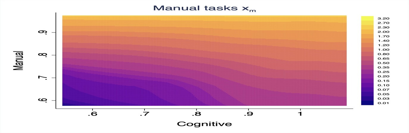
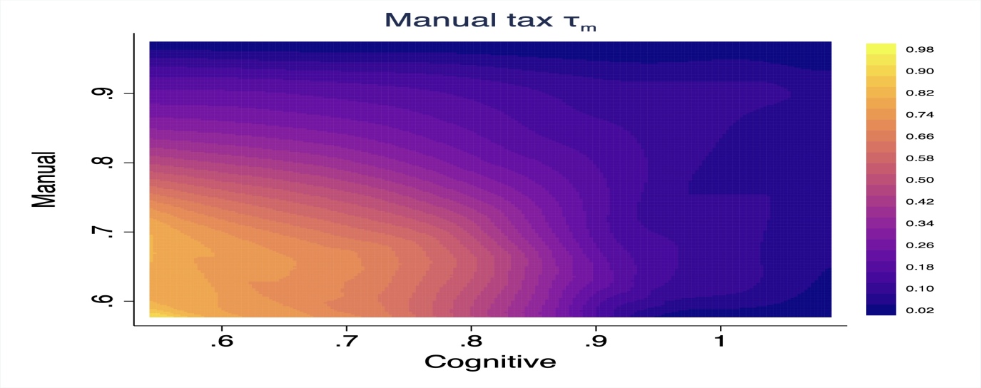
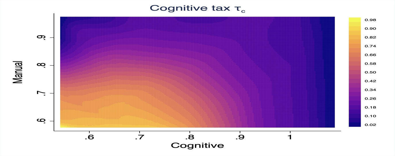
Figure A.2: Solution without Firm Heterogeneity

Figure A.2 shows the solution for the planner problem in an environment without firm heterogeneity. The top row documents the labor task and consumption allocation, the middle row shows optimal bunching, and the bottom row provides the optimal tax wedges. These panels are the equivalent of those in Figure 7, Figure 9, and Figure 11.

References

- (1)
- Abowd, Lengermann, and McKinney (2003) Abowd, J. M., P. Lengermann, and K. L. McKinney (2003): “The Measurement of Human Capital in the U.S. Economy,” U.S. Census Bureau Working Paper.
- Acemoglu and Autor (2011) Acemoglu, D., and D. Autor (2011): “Skills, Tasks and Technologies: Implications for Employment and Earnings,” in Handbook of Labor Economics, vol. 4, pp. 1043–1171.
- Ahlin (2017) Ahlin, C. (2017): “Matching Patterns when Group Size Exceeds Two,” American Economic Journal: Microeconomics, 9(1), 352–84.
- Alipour (2021) Alipour, P. (2021): “Optimal Income Taxation with Correlated Multi-Dimensional Preference Heterogeneity,” Pennsylvania State University Working Paper.
- Alvarez, Benguria, Engbom, and Moser (2018) Alvarez, J., F. Benguria, N. Engbom, and C. Moser (2018): “Firms and the Decline in Earnings Inequality in Brazil,” American Economic Journal: Macroeconomics, 10(1), 149–89.
- Ambrosio and Gigli (2013) Ambrosio, L., and N. Gigli (2013): “A User’s Guide to Optimal Transport,” in Modelling and Optimisation of Flows on Networks, pp. 1–155.
- Armstrong (1996) Armstrong, M. (1996): “Multiproduct Nonlinear Pricing,” Econometrica, 64(1), 51–75.
- Becker (1973) Becker, G. S. (1973): “A Theory of Marriage: Part I,” Journal of Political Economy, 81(4), 813–846.
- Benabou (2002) Benabou, R. (2002): “Tax and Education Policy in a Heterogeneous-Agent Economy: What Levels of Redistribution Maximize Growth and Efficiency?,” Econometrica, 70(2), 481–517.
- Blundell and Shephard (2012) Blundell, R., and A. Shephard (2012): “Employment, Hours of Work and the Optimal Taxation of Low-Income Families,” Review of Economic Studies, 79(2), 481–510.
- Boerma and Karabarbounis (2020) Boerma, J., and L. Karabarbounis (2020): “Labor Market Trends and the Changing Value of Time,” Journal of Economic Dynamics and Control, 115.
- Boerma and Karabarbounis (2021) (2021): “Inferring Inequality with Home Production,” Econometrica, 89(5), 2517–2556.
- Boerma, Tsyvinski, and Zimin (2021) Boerma, J., A. Tsyvinski, and A. P. Zimin (2021): “Sorting with Team Formation,” NBER Working Paper No. 29290.
- Bogachev and Kolesnikov (2012) Bogachev, V. I., and A. V. Kolesnikov (2012): “The Monge-Kantorovich Problem: Achievements, Connections, and Perspectives,” Russian Mathematical Surveys, 67(5), 785–890.
- Burk (1936) Burk, A. (1936): “Real Income, Expenditure Proportionality, and Frisch’s New Methods of Measuring Marginal Utility”,” The Review of Economic Studies, 4(1), 33–52.
- Card, Cardoso, and Kline (2016) Card, D., A. R. Cardoso, and P. Kline (2016): “Bargaining, Sorting, and the Gender Wage Gap: Quantifying the Impact of Firms on the Relative Pay of Women,” Quarterly Journal of Economics, 131(2), 633–686.
- Card, Heining, and Kline (2013) Card, D., J. Heining, and P. Kline (2013): “Workplace Heterogeneity and the Rise of West German Wage Inequality,” Quarterly Journal of Economics, 128(3), 967–1015.
- Chade and Eeckhout (2018) Chade, H., and J. Eeckhout (2018): “Matching Information,” Theoretical Economics, 13(1), 377–414.
- Chade, Eeckhout, and Smith (2017) Chade, H., J. Eeckhout, and L. Smith (2017): “Sorting through Search and Matching Models in Economics,” Journal of Economic Literature, 55(2), 493–544.
- Chetty, Guren, Manoli, and Weber (2012) Chetty, R., A. Guren, D. Manoli, and A. Weber (2012): “Does Indivisible Labor Explain the Difference Between Micro and Macro Elasticities? A Meta-Analysis of Extensive Margin Elasticities,” NBER Macroeconomics Annual, 27, 1–56.
- Chiappori, McCann, and Nesheim (2010) Chiappori, P.-A., R. J. McCann, and L. P. Nesheim (2010): “Hedonic Price Equilibria, Stable Matching, and Optimal Transport: Equivalence, Topology, and Uniqueness,” Economic Theory, 42(2), 317–354.
- Chiappori, McCann, and Pass (2017) Chiappori, P.-A., R. J. McCann, and B. Pass (2017): “Multi-to One-Dimensional Optimal Transport,” Communications on Pure and Applied Mathematics, 70(12), 2405–2444.
- Conesa, Kitao, and Krueger (2009) Conesa, J. C., S. Kitao, and D. Krueger (2009): “Taxing Capital? Not a Bad Idea After All!,” American Economic Review, 99(1), 25–48.
- Deming (2017) Deming, D. J. (2017): “The Growing Importance of Social Skills in the Labor Market,” Quarterly Journal of Economics, 132(4), 1593–1640.
- Diamond (1998) Diamond, P. A. (1998): “Optimal Income Taxation: An Example with a U-shaped Pattern of Optimal Marginal Tax Rates,” American Economic Review, 88(1), 83–95.
- Dupuy and Galichon (2014) Dupuy, A., and A. Galichon (2014): “Personality Traits and the Marriage Market,” Journal of Political Economy, 122(6), 1271–1319.
- Eeckhout (2018) Eeckhout, J. (2018): “Sorting in the Labor Market,” Annual Review of Economics, 10, 1–29.
- Ekeland and Moreno-Bromberg (2010) Ekeland, I., and S. Moreno-Bromberg (2010): “An Algorithm for Computing Solutions of Variational Problems with Global Convexity Constraints,” Numerische Mathematik, 115(1), 45–69.
- Galichon (2018) Galichon, A. (2018): Optimal Transport Methods in Economics. Princeton University Press.
- Galichon and Salanié (2021) Galichon, A., and B. Salanié (2021): “Cupid’s Invisible Hand: Social Surplus and Identification in Matching Models,” New York University Working Paper.
- Gayle and Shephard (2019) Gayle, G.-L., and A. Shephard (2019): “Optimal Taxation, Marriage, Home Production, and Family Labor Supply,” Econometrica, 87(1), 291–326.
- Golosov and Krasikov (2022) Golosov, M., and I. Krasikov (2022): “Multidimensional Screening in Public Finance: The Optimal Taxation of Couples,” University of Chicago Working Paper.
- Griessler (2018) Griessler, C. (2018): “C-cyclical Monotonicity as a Sufficient Criterion for Optimality in the Multimarginal Monge-Kantorovich Problem,” Proceedings of the American Mathematical Society, 146(11), 4735–4740.
- Guvenen, Karahan, Ozkan, and Song (2021) Guvenen, F., F. Karahan, S. Ozkan, and J. Song (2021): “What Do Data on Millions of US Workers Reveal about Lifecycle Earnings Dynamics?,” Econometrica, 89(5), 2303–2339.
- Guvenen, Kuruscu, Tanaka, and Wiczer (2020) Guvenen, F., B. Kuruscu, S. Tanaka, and D. Wiczer (2020): “Multidimensional Skill Mismatch,” American Economic Journal: Macroeconomics, 12(1), 210–44.
- Guvenen, Ozkan, and Song (2014) Guvenen, F., S. Ozkan, and J. Song (2014): “The Nature of Countercyclical Income Risk,” Journal of Political Economy, 122(3), 621–660.
- Heathcote, Storesletten, and Violante (2017) Heathcote, J., K. Storesletten, and G. L. Violante (2017): “Optimal Tax Progressivity: An Analytical Framework,” Quarterly Journal of Economics, 132(4), 1693–1754.
- Heathcote and Tsujiyama (2021a) Heathcote, J., and H. Tsujiyama (2021a): “Optimal Income Taxation: Mirrlees meets Ramsey,” Journal of Political Economy, 129(11), 3141–3184.
- Heathcote and Tsujiyama (2021b) (2021b): “Practical Optimal Income Taxation,” FRB of Minneapolis Working Paper.
- Judd, Ma, Saunders, and Su (2017) Judd, K., D. Ma, M. A. Saunders, and C.-L. Su (2017): “Optimal Income Taxation with Multidimensional Taxpayer Types,” Stanford University Working Paper.
- Karunamuni and Alberts (2005) Karunamuni, R. J., and T. Alberts (2005): “A Generalized Reflection Method of Boundary Correction in Kernel Density Estimation,” Canadian Journal of Statistics, 33(4), 497–509.
- Kleven, Kreiner, and Saez (2006) Kleven, H. J., C. T. Kreiner, and E. Saez (2006): “The Optimal Income Taxation of Couples,” NBER Working Paper No. 12685.
- Kleven, Kreiner, and Saez (2009) (2009): “The Optimal Income Taxation of Couples,” Econometrica, 77(2), 537–560.
- Kremer (1993) Kremer, M. (1993): “The O-Ring Theory of Economic Development,” Quarterly Journal of Economics, 108(3), 551–575.
- Lehmann, Renes, Spiritus, and Zoutman (2021) Lehmann, E., S. Renes, K. Spiritus, and F. Zoutman (2021): “Optimal Taxation with Multiple Incomes and Types,” CEPR Discussion Paper No. 16571.
- Lindenlaub (2017) Lindenlaub, I. (2017): “Sorting Multidimensional Types: Theory and Application,” Review of Economic Studies, 84(2), 718–789.
- Lindenlaub and Postel-Vinay (2022) Lindenlaub, I., and F. Postel-Vinay (2022): “Multidimensional Sorting under Random Search,” Yale University Working Paper.
- Lise and Postel-Vinay (2020) Lise, J., and F. Postel-Vinay (2020): “Multidimensional Skills, Sorting, and Human Capital Accumulation,” American Economic Review, 110(8), 2328–76.
- McAfee and McMillan (1988) McAfee, R. P., and J. McMillan (1988): “Multidimensional Incentive Compatibility and Mechanism Design,” Journal of Economic Theory, 46(2), 335–354.
- Mirrlees (1971) Mirrlees, J. A. (1971): “An Exploration in the Theory of Optimum Income Taxation,” Review of Economic Studies, 38(2), 175–208.
- Moser and Olea de Souza e Silva (2019) Moser, C., and P. Olea de Souza e Silva (2019): “Optimal Paternalistic Savings Policies,” Columbia Business School Working Paper.
- Oberman (2013) Oberman, A. M. (2013): “A Numerical Method for Variational Problems with Convexity Constraints,” SIAM Journal on Scientific Computing, 35(1), 378–396.
- Pollak (1971) Pollak, R. A. (1971): “Additive Utility Functions and Linear Engel Curves,” Review of Economic Studies, 38(4), 401–414.
- Rochet and Choné (1998) Rochet, J.-C., and P. Choné (1998): “Ironing, Sweeping, and Multidimensional Screening,” Econometrica, 66(4), 783–826.
- Rothschild and Scheuer (2013) Rothschild, C., and F. Scheuer (2013): “Redistributive Taxation in the Roy Model,” Quarterly Journal of Economics, 128(2), 623–668.
- Rothschild and Scheuer (2014) (2014): “A Theory of Income Taxation under Multidimensional Skill Heterogeneity,” NBER Working Paper No. 19822.
- Rothschild and Scheuer (2016) (2016): “Optimal Taxation with Rent-Seeking,” Review of Economic Studies, 83(3), 1225–1262.
- Roys and Taber (2022) Roys, N., and C. Taber (2022): “Skill Prices, Occupations, and Changes in the Wage Structure for Low Skilled Men,” University of Wisconsin Working Paper.
- Saez (2001) Saez, E. (2001): “Using Elasticities to Derive Optimal Income Tax Rates,” Review of Economic Studies, 68(1), 205–229.
- Sanders and Taber (2012) Sanders, C., and C. Taber (2012): “Life-cycle Wage Growth and Heterogeneous Human Capital,” Annual Review of Economics, 4(1), 399–425.
- Sattinger (1993) Sattinger, M. (1993): “Assignment Models of the Distribution of Earnings,” Journal of Economic Literature, 31(2), 831–880.
- Scheuer (2014) Scheuer, F. (2014): “Entrepreneurial Taxation with Endogenous Entry,” American Economic Journal: Economic Policy, 6(2), 126–63.
- Scheuer and Werning (2017) Scheuer, F., and I. Werning (2017): “The Taxation of Superstars,” Quarterly Journal of Economics, 132(1), 211–270.
- Shaked and Shanthikumar (2007) Shaked, M., and J. G. Shanthikumar (2007): Stochastic Orders. Springer Series in Statistics.
- Song, Price, Guvenen, Bloom, and Von Wachter (2019) Song, J., D. J. Price, F. Guvenen, N. Bloom, and T. Von Wachter (2019): “Firming Up Inequality,” Quarterly Journal of Economics, 134(1), 1–50.
- Villani (2003) Villani, C. (2003): Topics in Optimal Transportation, vol. 58. American Mathematical Society.
- Yamaguchi (2012) Yamaguchi, S. (2012): “Tasks and Heterogeneous Human Capital,” Journal of Labor Economics, 30(1), 1–53.