Prediction uncertainty validation for computational chemists
Abstract
Validation of prediction uncertainty (PU) is becoming an
essential task for modern computational chemistry. Designed to quantify
the reliability of predictions in meteorology, the calibration-sharpness
(CS) framework is now widely used to optimize and validate uncertainty-aware
machine learning (ML) methods. However, its application is not limited
to ML and it can serve as a principled framework for any PU validation.
The present article is intended as a step-by-step introduction to
the concepts and techniques of PU validation in the CS framework,
adapted to the specifics of computational chemistry. The presented
methods range from elementary graphical checks to more sophisticated
ones based on local calibration statistics. The concept of tightness,
is introduced. The methods are illustrated on synthetic datasets and
applied to uncertainty quantification data issued from the computational
chemistry literature.
This is the author’s version of the manuscript accepted for publication in The Journal of
Chemical Physics (AIP). The published version can be accessed at https://doi.org/10.1063/5.0109572
I Introduction
Uncertainty quantification (UQ) is becoming a major issue for chemical machine learning (ML),(Weymuth2022, ) notably for the prediction of molecular and material properties.(Janet2019, ; Musil2019, ; Scalia2020, ; Tran2020, ; Wang2021, ; Zhan2021, ; Imbalzano2021, ; Busk2022, ; Hu2022, ) This is also the case for quantum chemistry, when a level of confidence on predictions is sought out.(Pernot2015, ; DeWaele2016, ; Proppe2016, ; Pernot2017, ; Proppe2017, ; Pernot2017b, ; Proppe2019a, ; Lejaeghere2020, ; Proppe2022, ; Pernot2022a, ; Reiher2022, ; Weymuth2022, ) In these contexts, the validation of UQ outputs is essential to enable their use in applications such as active learning or actionable predictions for the industry.
The practice of validation methods in the computational chemistry (CC) UQ literature is quite diverse: from absent to elaborate through inappropriate. Even appropriate methods are found in several variants. There is clearly a lack of uniformity and of well-defined reference methods. The calibration-sharpness (CS) framework(Gneiting2014, ) provides a principled approach to ML-UQ validation.(Tran2020, ; Scalia2020, ; Busk2022, ) Scalia et al. (Scalia2020, ) distinguish two validation settings: (i) confidence- or intervals-based calibration,(Kuleshov2018, ) comparing the empirical coverage of prediction intervals to their intended confidence level; and (ii) error-based calibration,(Levi2020, ) comparing errors to their predicted dispersion (variance-based calibration would be more appropriate,(Kuppers2022, ) as both validation settings are based on error statistics, and I will use this denomination below).
In a recent article, noted thereafter PER2022,(Pernot2022a, ) I explored the application of the CS framework to the validation of CC-UQ. My goal was to derive a practical set of validation tools adapted to the specifics of CC-UQ, notably (i) the frequent use of statistical summaries (standard or expanded uncertainties),(Ruscic2014, ) instead of the prediction distributions expected by the CS framework, (ii) the possible presence of uncertainty on the reference data used for validation, (iii) the small size of most validation datasets when compared to ML applications, which limits the power of statistical tests, and (iv) the non-normality of the error distributions due to the frequent predominance of model errors.(Pernot2015, ; Pernot2018, ; Pernot2020b, ; Pernot2021, )
Considering these constraints, I was driven into considering two validation options for calibration, based on the available information. When expanded uncertainties are available, such as (the half-range of a 95% confidence interval, as recommended in thermochemistry(Ruscic2014, )), calibration should be tested by comparing the effective coverage of the corresponding prediction intervals to the target probability. But when standard uncertainties are available, the best option to avoid undue distribution hypotheses is to test the variance of z-scores (errors normalized by the corresponding uncertainty), which should be 1. This dichotomy maps perfectly the settings of Scalia et al. (Scalia2020, ), although implementation details may differ.
However, average calibration of a prediction uncertainty scheme over a validation set does not guarantee its small-scale reliability.(Kuleshov2018, ) When designing a prediction method, this is typically addressed by the consideration of sharpness, a statistic quantifying the concentration of predictive distributions. Within a set of calibrated method, one should prefer the sharpest one. However, even the sharpest one might still fail at small-scale reliability. This led me in PER2022 to propose local calibration analysis schemes (LCP and LZV methods), where calibration is assessed within subsets of the validation set. This is a form of group calibration(Chung2021, ) or multicalibration(HebertJohnson2017, ). I will show below how the LZV analysis relates also to the reliability diagrams introduced recently by Levi et al.(Levi2020, )
Being hampered by the lack in the CS framework of a concept qualifying small-scale or local calibration, I introduce below the tightness concept. As I found few to no use for sharpness in a pure validation context (it is mostly useful in the benchmarking or design of probabilistic prediction methods), I mostly refer in the following to a calibration-tightness (CT) framework.
A point that was not treated in PER2022 is the case where prediction statistics, typically mean and standard deviation, are based on small prediction ensembles. This is a frequent scenario in ML-UQ.(Smith2018, ; Zheng2022, ) The robustness of the calibration and tightness validation methods in presence of this source of statistical noise needed to be studied. Moreover, as the ML-UQ literature makes an abundant use of ranking-based statistics I also evaluated the interest of the correlation coefficients between uncertainty and absolute errors(Tynes2021, ) and the so-called confidence curves(Scalia2020, ) for CC-UQ validation.
The next section (Sect. II) presents a short overview of the concepts and validation methods. Its aim is to provide a step-by-step approach to the calibration-tightness UQ validation framework and enable, as far as possible, its use by non-statisticians. After this, readers new to the field might like to skip the technical sections (III-V) and go directly to Section VI for examples of application to a variety of CC-UQ datasets.
Sect. III introduces general definitions and notations used throughout the study and also the synthetic datasets used to illustrate the methods. Sect. IV presents simple graphical validation checks that do not require statistical testing procedures. These might be used for screening out problematic UQ outputs. Unfortunately, quantitative validation is often necessary to conclude in situations where rejection of calibration or tightness is not clear cut. Quantitative methods for ranking-, intervals- and variance-based methods are presented in Sect. V, with the necessary statistical tools and derived graphics. Sect. VI presents applications of these tools to datasets from the CC-UQ literature. Available software implementing the CS and CT frameworks, or parts of them, is presented in Sect. VII. A conclusive discussion is presented in Sect. VIII.
II A short guide to CC-UQ validation
This section provides a brief introduction to the concepts and methods for UQ validation in computational chemistry, by guiding potential users to the choice of methods best adapted to their data. Without further delving into the technical details, readers new to this topic should then be able to understand the case studies presented in Section VI, and to appreciate the interest and usefulness of these tools. Links to the main text are provided for each topic. For bibliographic references, please consult the relevant sections.
To begin with, one needs a validation set, which can be as minimal as a set of errors () and the corresponding dispersion statements. Errors are the differences between predicted values of a quantity of interest (QoI) and reference values, and dispersion statements on errors can take the form of predictive distributions, prediction ensembles or statistical summaries, typically uncertainties. Note that these should account for the dispersion of reference values, if any. [Sect. III.2]
The goal of calibration validation is to check the statistical consistency between the errors and their dispersion statements. One considers two complementary validation levels: average calibration (simply referred-to below as calibration), where the statistical consistency is checked over the whole validation set, and tightness, where the statistical consistency is checked at a finer scale, typically in relevant subsets of the validation set. Calibration alone does not guarantee the reliability of individual prediction uncertainties, and tightness should be sought for. Note that a set of predictions cannot be considered to be tight if it is not calibrated. [Sect. III.1]
Many validation methods are proposed in the literature. The most important decision criterion to choose a pertinent method is based on the available dispersion information. The main types occurring in CC-UQ (uncertainty, expanded uncertainty, prediction ensembles and predictive distributions) are considered now to present the available options.
Uncertainty.
Let us consider first a very common scenario, where one has a set of errors and uncertainties, noted and . Without further characterization, an uncertainty has to be understood as a standard uncertainty, i.e. the standard deviation of the possible values of the corresponding property. Hence, the basic probabilistic model linking an error to an uncertainty is , meaning that is a random realization from an unspecified distribution , centered on 0 (errors are assumed to be corrected of systematic bias) with scale/dispersion parameter . One should thus consider distribution-free validation methods, and simply answer the question: “Does uncertainty correctly quantify the dispersion of the errors ?”. [Sect. V.1.1]
-
•
If one deals with a constant value of (homoscedastic case), one cannot do much better than to check that correctly describes the variance of the errors set, i.e. or for , within the limits allowed by the size of the validation set . Note that this is a test for (average) calibration and this simple scenario does not enable to assess tightness. For this, one would need to have additional data, such as the set of predicted values from which is derived, and check that in relevant subsets of . This is called a local Z-variance (LZV) analysis. [Sect. V.2.2]
-
•
If is not constant (heteroscedastic case), a simple graphical method, where one plots vs can help to answer the main question (Fig. 1): if on such a plot the dispersion of does not increase linearly with , the statistical consistency can be rejected without further trial. In the opposite case, additional tests are necessary to assess calibration and tightness. [Sect. IV.1] For calibration, one should check that . For tightness, validation methods use the estimation of error statistics within subsets of sorted values:
- –
- –
-
–
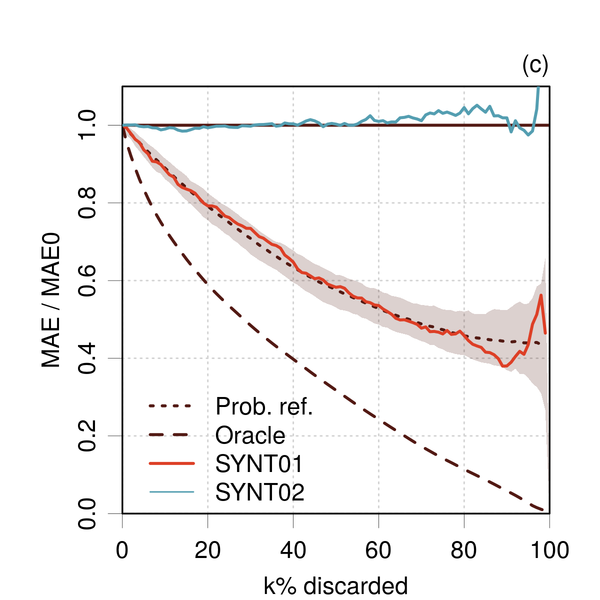
In confidence curves [Fig. 5(c)], one makes sets of errors iteratively pruned from the values associated with an increasing percentage of the largest uncertainties. The mean absolute error (MAE) for those sets is plotted against the percentage of pruning. A uniformly decreasing curve reveals that the larger absolute errors are associated with larger uncertainties, but it does not inform us on a proper scaling. To assess tightness, one needs to compare the confidence curve to a probabilistic reference curve obtained by the same procedure using a synthetic dataset of errors generated using the probabilistic model. [Sect. V.1.3]
In complement to a calibration test (for instance ), a reliability diagram and a LZV analysis provide basically the same information and enable to validate tightness. In the case of a confidence curve, a probabilistic reference is required to reach the same goal, which implies a choice of distribution for . As in the homoscedastic case, if the predicted values () are also available, tightness can be tested by a LZV analysis using subsets of .
Expanded uncertainty.
A less common scenario is based on expanded uncertainties (), which are the half range of a probability interval (typically at the % level). Without information on the distribution of prediction errors, one cannot reliably estimate a standard uncertainty from an expanded uncertainty, and the variance-based validation methods proposed above cannot be used. One should then have recourse to intervals-based validation methods. [Sect. V.1.1]
The prediction interval coverage probability (PICP) is estimated as the percentage of errors lying within the corresponding interval . For a good calibration, one should have , within the statistical uncertainty due to the size of the dataset. Applied to the whole validation set, this approach enables to validate calibration. For tightness, the same test is performed within subsets of the validation set, either along if it is not constant, and/or , if available, resulting in a local coverage probability (LCP) analysis [Fig. 4(a,b)]. [Sect. V.2.1]
Prediction ensembles.
Let us now consider ensemble-based dispersion assessments, which are common in ML-UQ. One has then an ensemble of errors for each prediction, from which to extract statistics.
For small ensembles (less than several hundred points), it is illusory to get reliable prediction intervals, and it is recommended to estimate as the standard error of an ensemble and use variance-based validation methods as described above. Note that for very small ensembles (smaller than 10 points) further complications arise, as the estimation of is itself very uncertain, and getting calibration/tightness diagnostics might be unrealistic. [Sect. V.3]
For large ensembles, one has the choice to use either intervals- and/or variance-based validation methods. In the case of intervals-based validation, a set of target probability levels can be tested in order to validate the shape of the prediction distribution. This multiple intervals-based calibration test is much more stringent than a variance-based validation.
Often, ML prediction ensembles are used for active learning more than for estimating prediction uncertainty. In such cases, the confidence curve is an interesting tool: a continuously decreasing confidence curve is sufficient to validate that a ML algorithm enables reliably to identify predictions with potentially large errors.
Predictive distributions.
Some ML methods provide for each prediction a distribution (typically normal) with is mean and dispersion parameters. As for large prediction ensembles, the full panel of variance- and intervals-based validation methods is accessible. Additionally, calibration curves are commonly used in this scenario to assess average calibration, but they do not enable to test tightness [Sect. V.2]. Note that a failure of intervals-based validation might be due either to the choice of distribution and/or to its estimated parameters, which complicates the diagnostic.
III Concepts, definitions and notations
III.1 Concepts and definitions
In order to validate the calibration of a prediction model or algorithm, one needs a validation set, composed of predicted values, their dispersion assessments, and reference values to compare with. Dispersion assessments can take the form of predictive distributions, prediction ensembles or statistical summaries, typically uncertainties.
Uncertainty.
Let us first recall the definition of uncertainty in metrology(GUM, ): “a non-negative number that quantifies the dispersion of the values being attributed to a quantity of interest” (QoI, noted ). Depending on the statistic used to quantify the dispersion, one distinguishes between standard uncertainty (noted thereafter), for which the dispersion is estimated by a standard deviation(GUM, ), and expanded uncertainty (noted thereafter), for which the dispersion is estimated by the half range of a probability interval, typically at the 95 % level ().(Ruscic2014, ) It is important to note that designing a probability interval from a standard uncertainty requires information on the QoI distribution, while no additional information is required for an expanded uncertainty.111Recently introduced,(Cox2022, ) characteristic uncertainty is estimated by . This proposition covers the gap between and in terms of information needed for prediction interval design.
Error.
In the UQ validation framework, the quantity of interest is the prediction error, i.e. the difference between a predicted value and a reference value. Different error sources might be characterized by specific uncertainties (numerical, parametric, model, aleatoric, epistemic…).(Lejaeghere2020, ) The prediction error should aggregate all the underlying error sources and, in absence of ambiguity, will be referred to simply as the error. The prediction uncertainty, which is the uncertainty on the prediction error, should thus provide a scale for the dispersion of prediction errors. This offers us a rationale for its validation, as presented in Sect. IV.1.
Calibration.
The calibration-sharpness (CS) framework(Gneiting2014, ) provides definitions for major concepts. Calibration estimates the “statistical compatibility of probabilistic forecasts and observations; essentially, realizations should be indistinguishable from random draws from predictive distributions”(Gneiting2014, ) where a probabilistic forecast or probabilistic prediction, provides a distribution over the values that can be taken by a QoI. In this framework, calibration is generally understood as average calibration, i.e. the calibration estimated over the full validation set. It is well understood that average calibration is insufficient to guarantee useful predictions.(Kuleshov2018, ; Pernot2022a, )
Sharpness.
In the optimization framework of UQ methods, sharpness metrics are used to identify more concentrated predictive distributions. Sharpness is defined as “the concentration of a predictive distribution in absolute terms; a property exclusive to the forecasts”.(Gneiting2014, ) Sharpness metrics are typically average dispersion statistics (mean prediction uncertainty or variance,(Kuleshov2018, ; Tran2020, ) or mean prediction interval width(Chung2021, ; Lai2022, )), that do not involve the reference values. As such, sharpness is barely relevant to UQ validation.
Tightness.
Stronger calibration concepts have been introduced to palliate the limitations of average calibration to describe the small-scale reliability of predictions to observations: individual calibration (calibration over each element of the validation set);(Chung2020, ) group calibration (calibration over pertinent groups of the validation set);(Chung2021, ) adversarial group calibration (calibration over randomly generated groups of the validation set);(Chung2021, ) and local calibration (calibration over groups mapping a pertinent feature).(Pernot2022a, ) Local calibration has to be understood as a form of group calibration (Chung2021, ) or multicalibration (HebertJohnson2017, ), based on the sub-setting of a continuous feature into adjacent or overlapping intervals. Its purpose is to identify local or small-scale departures from calibration which might have a diagnostic interest. When the mapping feature is prediction uncertainty, local calibration is tightly related to reliability diagrams (agreement of uncertainty with the dispersion of errors), which is also referred to as perfect calibration.(Levi2020, )
As sharpness cannot be used to characterize this small-scale reliability, I propose to use instead tightness as a dedicated concept to characterize the small-scale adaptation of UQ predictions to reference values. More widely, a set of predictions can be considered to be tight if it satisfies the requirements of any of the stronger calibration concepts (individual, group, local or perfect calibration). This offers a convenient shortcut for propositions such as group calibrated, locally calibrated or perfectly calibrated.
Note that it is tempting to assume that tightness implies average calibration. However, statistical uncertainty on calibration statistics for small groups might lead to scenarios where one accepts tightness while rejecting average calibration. As for sharpness, it is therefore important for tightness to be conditional to average calibration: a probabilistic prediction method cannot be tight if it is not (average) calibrated.
III.2 Notations
Prediction.
Let us consider a QoI, , for which one wants to make predictions with some form of confidence assessment. For a probabilistic prediction, the predictive distribution on can be characterized by its quantile function , where is a probability (the quantile function is the inverse of the cumulative distribution function).
However, few UQ methods provide predictive distribution functions, and empirical approximations are more often accessible from ensembles or samples, representative of the predictive distribution. In such cases, the standard uncertainty is estimated by the standard deviation of the sample,(GUM, ) and the expanded uncertainty from the empirical quantiles(Wilcox2012, ; Wilcox2018, )
| (1) |
where, to conform with usual notations, is the percentage corresponding to ().
The most frequent scenario in the computational chemistry UQ literature is to have a single statistical summary – very commonly the standard uncertainty and more rarely the expanded uncertainty .(Ruscic2014, ) The consequences of the absence of predictive distribution on the CS validation framework are explored below.
Validation.
For the sake of validation, predictions of , , are made for a series of test systems for which one has reference values . For each validation system , one needs at least one UQ object among , , or as defined above. Validation is made by assessing the statistical compatibility between the errors and the corresponding dispersion statements.
The minimal validation set is thus composed of errors and the corresponding UQ estimators, for instance , where if the reference data are not uncertain. When the reference values are themselves uncertain, this has to be propagated to the errors. For instance, if has a standard uncertainty and a standard uncertainty , the uncertainty on is obtained by combination of variances (considering that and are statistically independent).(GUM, ) Alternative combination schemes have to be considered for other types of uncertainty.(Pernot2022a, ) Note that if the uncertainty on the reference values contributes significantly to the uncertainty on , failure of validation tests might be difficult to interpret, as they might occur as well from the predictor as from the reference data.
Prediction intervals are at the center of the CS validation framework. A % error prediction interval can be estimated from the quantile function or its empirical variant () as
| (2) |
If one assumes the symmetry of intervals around , expanded uncertainties can also be used directly, i.e.
| (3) |
A contrario, it is not possible to design a prediction interval form a standard uncertainty without making hypotheses on the error distribution. Being mostly dominated by model errors, computational chemistry error distributions are often non-normal,(Pernot2020b, ; Pernot2021, ) which prevents the use of simple recipes (such as the rule). Making unsupported distribution hypotheses would add a fragility layer to the validation process, complicating the interpretation of negative validation tests. This prevents the application intervals-based validation to sets of standard uncertainties, and the use variance-based methods, such as reliability diagrams(Levi2020, ) of -scores () statistics(Pernot2022a, ), has been proposed as an alternative.
Intervals- and variance-based CT validation methods are presented in Sect. V.
III.3 Synthetic datasets
The methods presented below are illustrated on synthetic validation sets , with . is sampled uniformly in the interval . The SYNT01 errors are obtained from a probabilistic model
| (4) |
where is a probability density function with mean and standard deviation . This dataset is tagged as consistent, as errors and uncertainties are statistically consistent and should provide positive calibration and tightness tests. The other sets (SYNT02 and SYNT03) do not derive directly from this probabilistic model and are labeled as non-consistent.
- SYNT01
-
heteroscedastic consistent set, where the errors are generated from a zero-centered normal distribution with a standard deviation depending on , through .
- SYNT02
-
heteroscedastic non-consistent set, with errors sampled from a normal distribution and the same uncertainties as in SYNT01.
- SYNT03
-
homoscedastic non-consistent set, with errors taken from SYNT01 and constant .
IV Basic graphical methods
Considering a minimal validation set , it is possible to draw simple graphs to check that uncertainty quantifies correctly the dispersion of errors. One has to consider two cases: (1) varies notably over the validation set (heteroscedastic set); and (2) is (nearly) constant (homoscedastic set).
IV.1 Heteroscedastic validation sets
The consistency between errors and uncertainties (Eq. 4) is based on an asymmetrical relation, which can be summarized as follows
| (5) | ||||
| (6) |
i.e. large errors should occur only from predictions with large uncertainties and predictions with small uncertainties should be associated with small errors. The asymmetry results from the fact that small errors might arise as well from predictions with small uncertainty as from predictions with large uncertainty. In consequence, one should not expect a strong correlation between absolute errors and uncertainties (see Sect. V.1.3) and there is not much to learn from plots of vs .
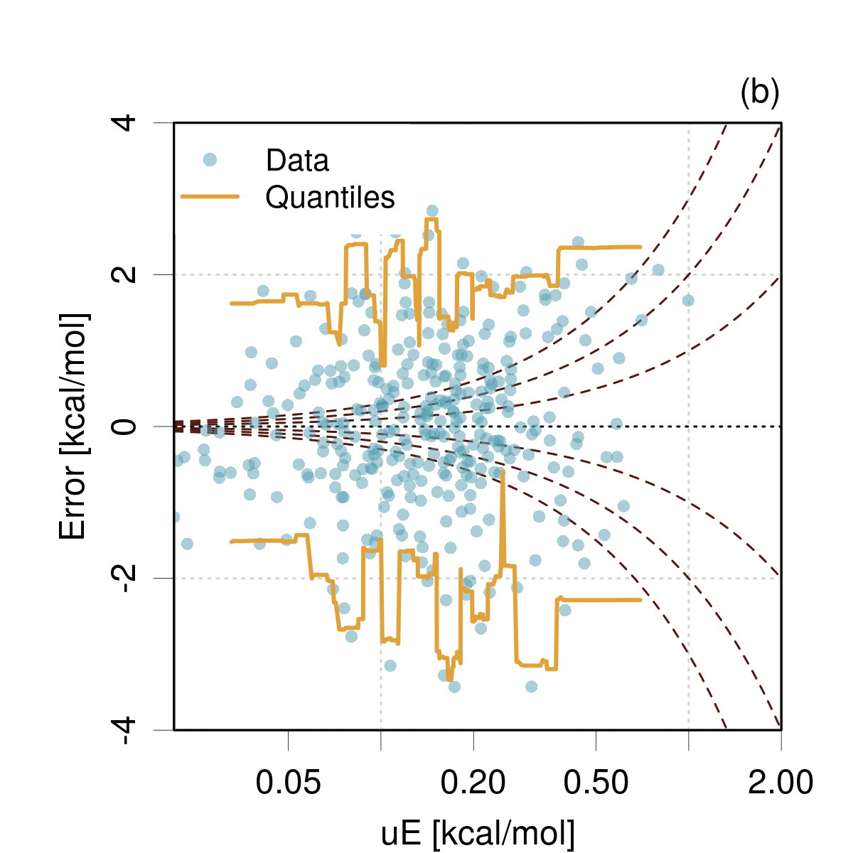
Basic plot.
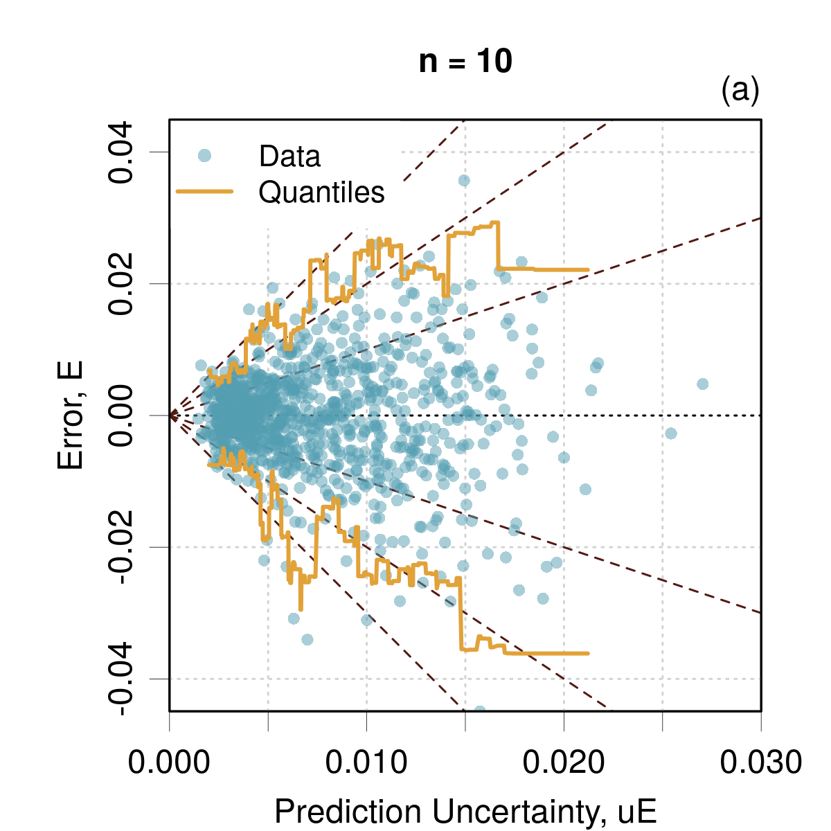
When depends notably on the validation point, one can simply plot vs to check how the dispersion of scales with .(Janet2019, ) An example is shown in Fig. 1(a), where guiding lines have been added to facilitate the appraisal of the expected linear scaling. One sees indeed for the consistent dataset SYNT01 that larger errors are associated with larger uncertainty values, giving a typical fan-like structure to the data cloud. The symmetry of the cloud with respect to the axis is furthermore a good indication that the errors have no noticeable bias.
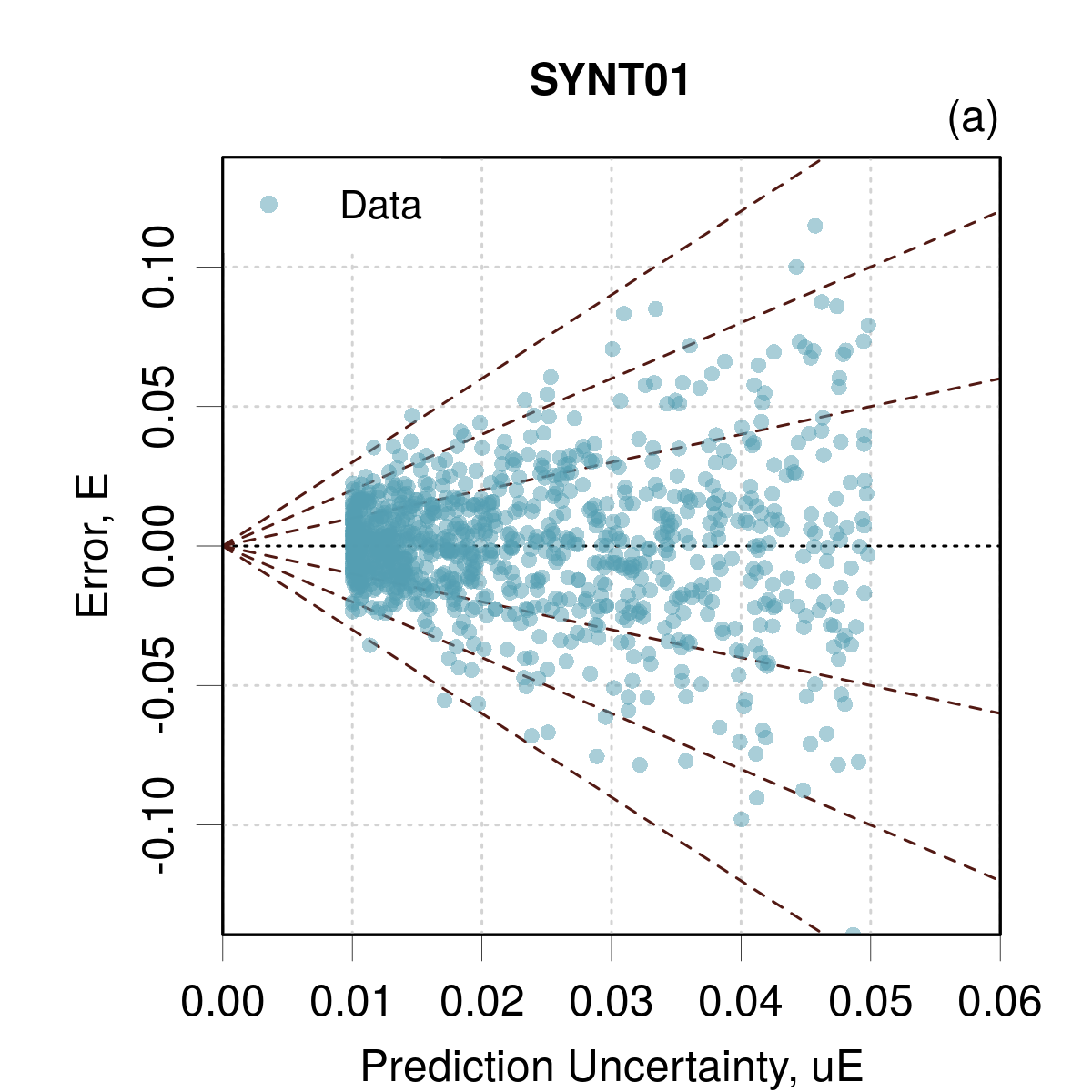
Improvements.
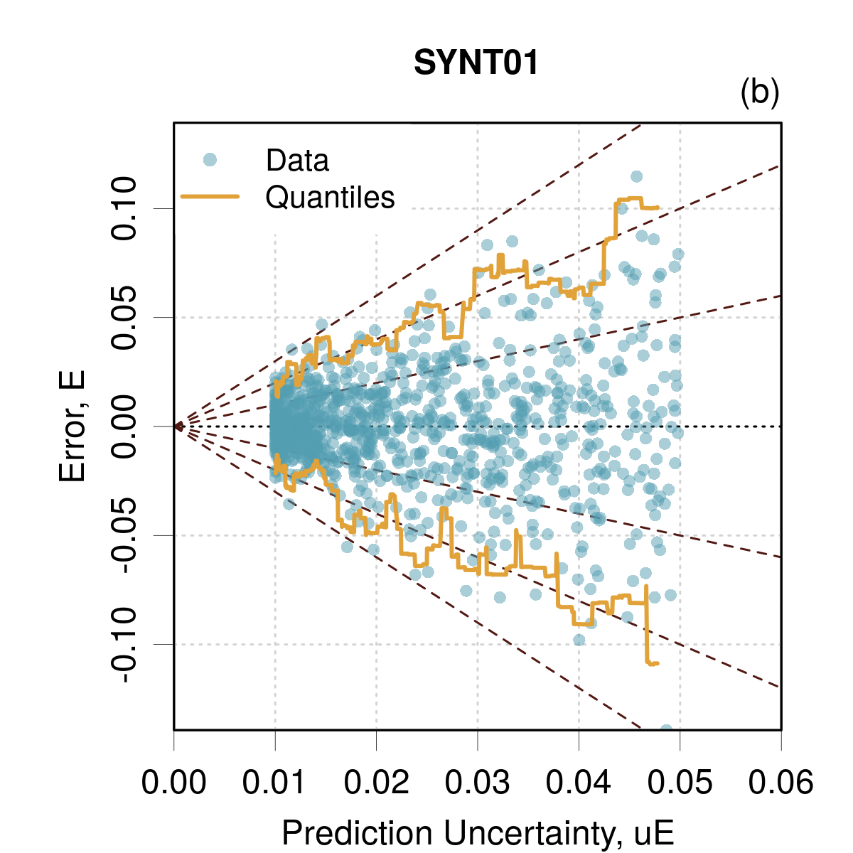
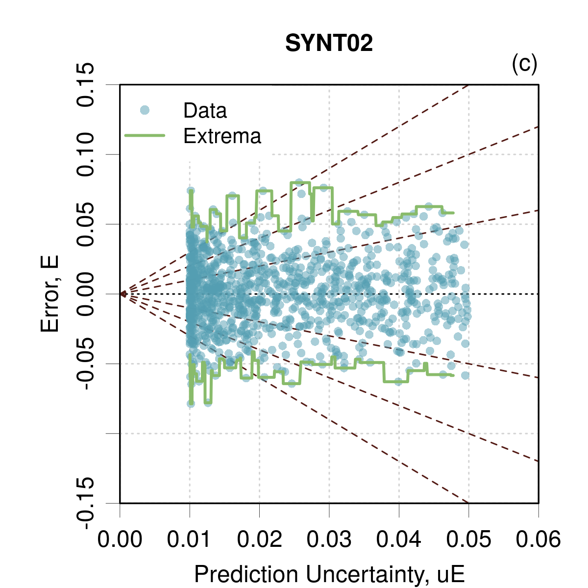
The proper scaling of with can be difficult to appreciate visually for small datasets. A little more sophisticated approach consists in adding an estimator of the local range of on the graph. This might be done by using a sliding window to estimate either the extrema or the limits of a 95 % probability interval. The latter method is called running quantiles and is depicted in Fig. 1(b). In this implementation, the sliding window contains a fixed number of points (not a fixed width of ), which is automatically estimated by using the Rice formula for histograms . One sees in Fig. 1(b) that the quantile lines oscillate around the lines, which can be expected from the properties of the normal distribution used to generate the SYNT01 dataset. In the case of the non-consistent SYNT02 dataset, Fig. 1(c) shows clearly the absence of scaling between and (the larger errors occur anywhere along the axis). This trend is underlined in this plot by running extrema lines, which are easier to compute than quantiles, but oscillate more strongly (strong dependence to outliers) and might be more difficult to interpret.
An alternative representation, plotting vs. , is used in the literature.(Musil2019, ) It is motivated by the fact that, for a normal error distribution with mean 0 and variance , the probability density function of the logarithm of absolute errors has its mode at . In these conditions, one should observe a strong concentration of points along the identity line for statistically consistent validation sets and a running mode line should lie close to it. It is important to understand the logic behind this type of plot, but I did not develop it further here because (i) it is less intuitive than the plot, (ii) it requires the estimation of the mode (or some high density levels of the data cloud) which limits the application to large datasets, and (iii) it is sensitive to deviations from the zero-centered normal error distribution which complicates the interpretation of a negative diagnostic.
IV.2 Homoscedastic validation sets
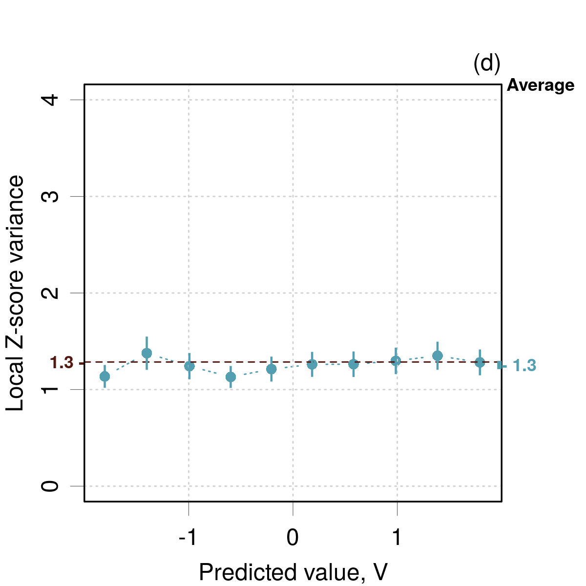
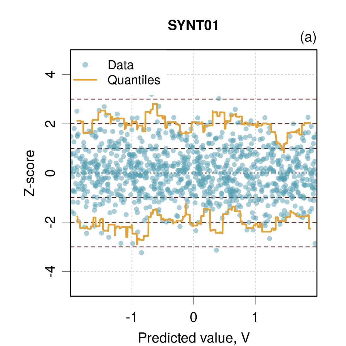
The problem when is constant is that the plot proposed above cannot be used. In such cases, the expected scaling can be appreciated by using -scores and plotting them against a relevant feature of the dataset, for instance the points index or the QoI . The latter is good to appreciate systematic trends in scaling and to relate them to a range of predicted values. Note that it might be difficult or impossible to spot z-score problems on such plots if they are not localized in space.
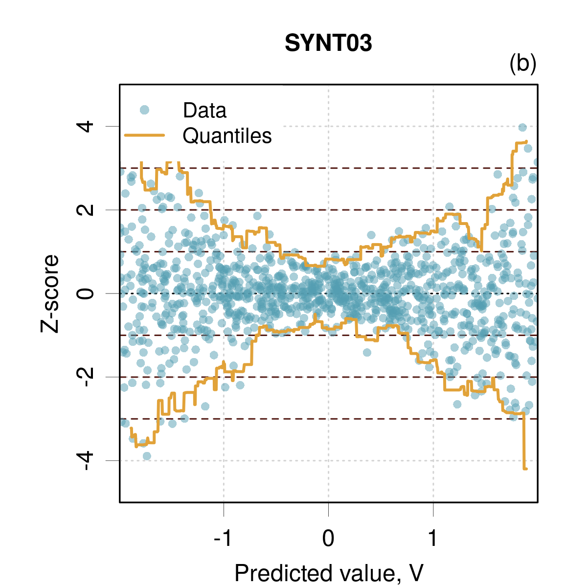
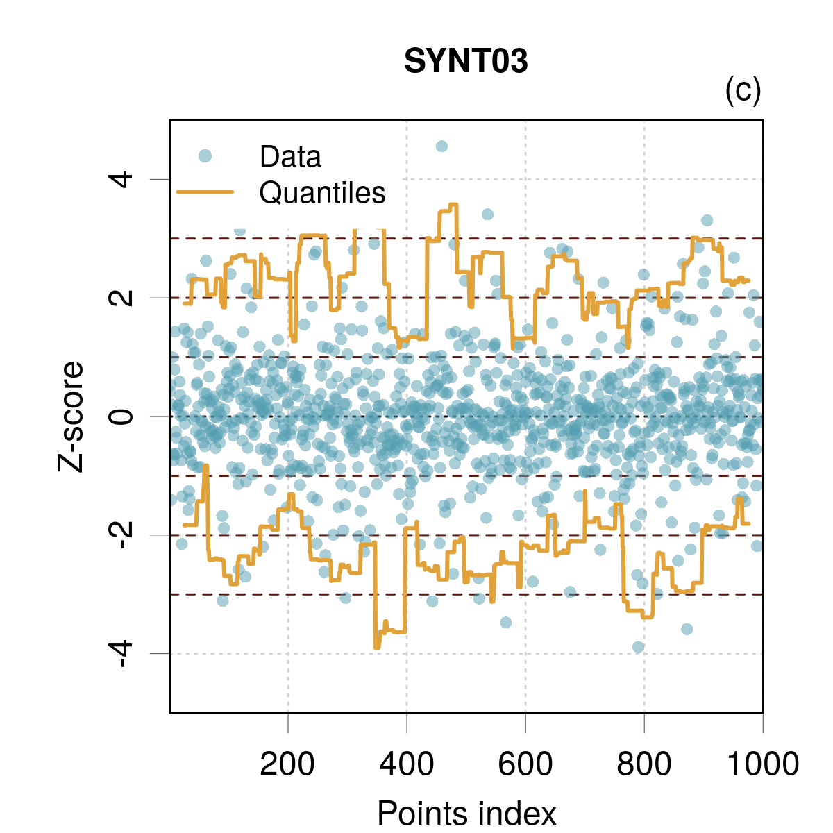
The guiding lines are now horizontal (), and, as above, a simple plot can be improved by running statistics. The running quantiles lines should run parallel to the guiding lines. An example is shown in Fig. 2(a) for an heteroscedastic consistent dataset (SYNT01). In Fig. 2(b) for a homoscedastic non-consistent dataset (SYNT03), the envelope of the data clearly deviates from the guiding lines. Although calibration is difficult to assess, one might safely conclude to a lack of tightness. Note that the diagnostic depends on the choice of a plotting ordinate. Fig. 2(c) presents the same dataset as a function of the point index. The non-reliability of the uncertainties is difficult to appreciate on this plot, as the running quantiles follow more or less the guiding lines, although with large oscillations when compared to the SYNT01 case.
IV.3 Remarks
-
•
These simple graphical methods should help to detect frank departures from calibration/tightness. They cannot be used to validate these properties. In cases where one cannot easily reject the consistency between errors and uncertainties, calibration and tightness have to be assessed by quantitative methods described below.
-
•
They are applicable to both standard () and expanded () uncertainties, albeit with different interpretations of the guiding lines.
- •
-
•
To lessen the dependence of the running statistics on a specific validation set, one might think of a bootstrapping(Efron1979, ; Efron1991, ) approach to estimate mean running statistics and their uncertainty. However, this might be a little far fetched for this simple qualitative visualization.
V Quantitative methods
V.1 Statistical framework
V.1.1 Average calibration
Intervals-based testing.
In the CS framework, a method is considered to be calibrated if the confidence of its predictions matches the probability of being correct for all confidence levels,(Tran2020, ; Tomani2021, ) which can be reformulated as “prediction intervals should have the correct coverage”.(Kuleshov2018, )
It is convenient here to deal with prediction errors instead of predicted values, and one defines the prediction interval coverage probability (PICP) as 222Note that this definition differs from the one in the calibration/sharpness literature (see e.g. Kuleshov et al.(Kuleshov2018, )) by my consideration of reference data uncertainty in the prediction interval.
| (7) |
where is the indicator function for proposition , taking values 1 when is true and 0 when is false, and is a % prediction interval for . Hence, estimating a PICP simply amounts to count the number of times a validation error falls within the corresponding prediction interval.
Using PICPs, a method is calibrated if(Kuleshov2018, )
| (8) |
In practice, one has a limited amount of validation data to test the equality, and a standard procedure to validate is to estimate a 95 % confidence interval on the statistic, , and to test if it contains :
| (9) |
The stacked notation is used as a shorthand for “does belong to ?”. Note that in the CC-UQ literature one often has to accept a weaker form of calibration, based on a single value (0.95).
is the bounded ratio of two integers () and is known in the literature as a binomial proportion.(Vollset1993, ) The finite set of realizable values for depends on , and it might not contain a given value of . There are many methods to estimate , with competing features such as optimal coverage or minimal range, and the choice of the best one is debated among experts. The main difficulty is that some properties of the confidence interval are sharply oscillating with , so that the best choice might depend on . However, all the experts agree that the textbook method (known as the Wald method), based on a normality hypothesis, has to be avoided.
An exploratory comparison (Pernot2022a, ) over a set of methods available in the R language(RTeam2019, ) showed that it is reasonable in the present setup to choose between the Agresti-Coull (Agresti1998, ), Clopper-Pearson (Clopper1934, ) and continuity-corrected Wilson (Newcombe1998, ) methods. The latter is my standard choice in this study.
A limitation of PICP testing is the saturation of the coverage at the upper limit: if a prediction interval for achieves a coverage probability , one gets no information on the amplitude of the mismatch with the target probability. As a complementary diagnostic, I find useful to consider the ranges ratio (RR), i.e. the ratio of the mean range of prediction intervals over the range of the empirical interval at probability :
| (10) |
where is the upper/lower limit of a prediction interval and is the empirical quantile function of errors, estimated over the validation set (not to be confounded with which is defined for individual predictions). Deviations of from unity quantify the mismatch amplitude. The effect of the validation set size on the value of can be estimated by bootstrapping.(Efron1979, ; Efron1991, )
A second limitation of PICP testing appears when one has no sufficient information to design a reliable prediction interval. This occurs, frequently, when only standard uncertainties are available, in absence of information on the underlying error distribution. In such cases, one should turn to variance-based validation.
Variance-based testing.
The underlying probabilistic model for variance-based testing is given by Eq. 4. Hence, for homoscedastic data, the consistency between errors and uncertainty can readily be checked by comparing the error variance to the squared uncertainty
| (11) |
To extend this equation to heteroscedastic data, let us assume that the errors are drawn from a distribution (Eq. 4) with a scale parameter distributed according to . The distribution of errors is then a compound distribution, more specifically a scale mixture distribution. The variance of the compound distribution is obtained by the law of total variance, i.e.
| (12) |
The first term of the RHS can be estimated as the mean squared uncertainty . For unbiased errors, the second term of the RHS should be small to negligible, but in a general case, its estimation requires binning of the errors according to the corresponding uncertainties, estimating the mean error in each bin and taking the variance of the mean errors over the bins. Accuracy of this procedure depends on the sample size and binning strategy, and the main limitations of this technique are the same as advanced by Scalia et al.(Scalia2020, ) for the application of reliability diagrams (see Sect. V.1.2). Besides these technical complications, the test for unbiased errors would thus be
| (13) |
which does not account for the essential pairing between errors and uncertainties, and could enable fortuitous agreements, i.e. an equality does not guarantee that the probabilistic model (Eq. 4) is respected by the data.
For heteroscedastic data, it seems thus more reliable to use scaled uncertainties, or -scores , which account for the pairing between errors and uncertainties, and for which Eq. 13 becomes
| (14) |
Note that this test is valid for both homoscedastic and heteroscedastic data.(Pernot2022a, ) In the hypothesis of unbiased errors, one should also have . Formally, can be linked to the Birge ratio used in metrology to test statistical consistency.(Birge1932, ; Kacker2010, ; Bodnar2014, ) See Appendix A for more details.
Following the same logic as for PICPs, practical validation of relies on the test
| (15) |
where can be estimated by an adapted bootstrapping method (BCa, ABC…) to avoid the normality-based textbook method.(DiCiccio1996, ) A faster, but slightly less accurate method to estimate is based on the estimation of introduced by Cho et al. (Cho2005, ), using the central moments of the sample
| (16) |
where and is the arithmetic mean of . In absence of further information on the distribution of , a normality hypothesis leads to the test
| (17) |
where denotes the upper and lower bounds of the interval, and is the % quantile of the Student’s- distribution with degrees of freedom. The symmetry of the testing interval might be problematic for small values, but in most scenarios tested in PER2022, this method performed nearly as well as the best bootstrapping methods and better than the worst ones.(Pernot2022a, ) Moreover, it is much faster.
Statistical power.
The efficiency of the tests described above depends on the size of the validation set. The power of the test is the probability to correctly reject the hypothesis that a PICP or Var(Z) value is compatible with its target value. A power threshold (typically 0.8) is defined to determine a minimal sample size.
Fig. 3 reports the minimal sample sizes necessary to reach a power of 0.8 for differences between a PICP value and its target value (see also PER2022(Pernot2022a, ) (Fig. S2) for an alternative representation). For instance, a sample size of is necessary to achieve a power of 0.8 in differentiating a PICP value of from its target. Rejecting safely a difference would take more than 2000 points for the same target. The situation worsens for smaller target values (above 0.5, which is a symmetry point): for , one needs about 800 points to reject the compatibility between and .
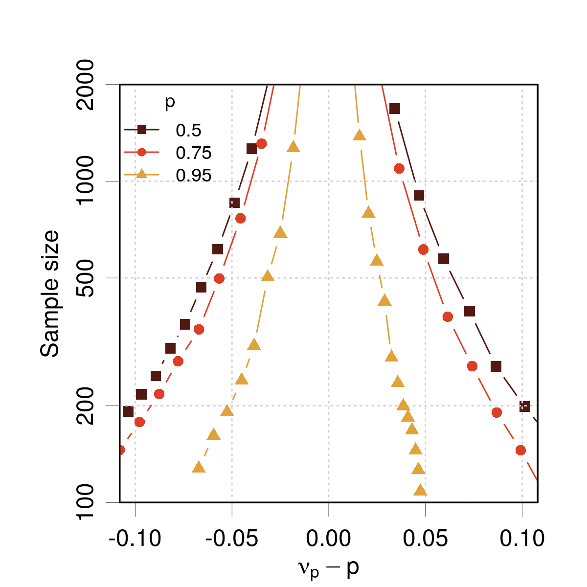
As a guiding rule, similar sample sizes are required to test .
V.1.2 Tightness
As evoked previously, using the tests presented above on a validation set provides only an average calibration diagnostic, which is not sufficient to guarantee the desired tightness of prediction intervals, i.e. the small-scale reliability of the probabilistic predictions.
Local calibration.
A simple way to assess tightness is to split the dataset into groups of sizes and test the average calibration for each group. For PICPs, one should therefore test
| (18) |
with a similar formula for .
The focus is here on the design of contiguous or overlapping groups partitioning some relevant feature. In this case, tightness is similar to local calibration. In contrast to randomly generated groups used for adversarial group calibration, local calibration enables a diagnostic of tightness problems in specific areas of the grouping feature. For continuous grouping features, several designs can be considered: contiguous groups, overlapping groups or a sliding window. For the kind of datasets we are considering in this study, the features of choice to design groups are typically the predicted value and the prediction uncertainty ( or ) for heteroscedastic validation sets. This approach leads to the local coverage probability (LCP),(Pernot2022a, ) local variance (LZV)(Pernot2022a, ) and local range ratio (LRR) analyses used in the graphical representations described below.
Reliability diagram.
To compare the uncertainty to the error, Scalia et al. (Scalia2020, ) considered the proposition of Levi at al.(Levi2020, ) to use a generalization of Eq. 11 in order ascertain the conformity of the empirical error variance with the predicted one, i.e.
| (19) |
where, for each value of , the variance is estimated on those points of the validation set having as predicted variance. The practical implementation of this scheme, resulting in a so-called reliability diagram, requires binning of values into intervals of . For each bin one plots the standard deviation of the corresponding errors, noted , vs the root of the mean squared value of the selected data, noted . Its applicability, as for Eq. 12, is limited by low bin counts, notably for small validation sets or those with highly skewed uncertainty distributions.(Scalia2020, ) Note that this formulation is closely related to the LZV analysis, but instead of estimating for binned values of , one estimates , with the same caveat about the neglect of pairing between and values as for Eq. 13.
Levi et al.(Levi2020, ) demonstrated the advantage of their method over the intervals-based approach of Kuleshov et al.(Kuleshov2018, ). I want to emphasize here that both methods do not test for the same “calibration”. The former one tests for tightness (Levi et al. speak of perfect calibration), where the latter one tests for average calibration. I think that one interest of the tightness concept is to make such a distinction more legible.
Statistical power.
The sizes of the groups should ideally be large enough to retain sufficient testing power, which in some cases might limit the number of groups and the resolution of the tightness analysis. For small validation sets, the use of overlapping groups, and notably a sliding window design, enables to preserve diagnostic resolution without loosing too much testing power.
Smaller groups mean wider confidence intervals for local statistics, and one might find situations where the average calibration is rejected, while it seems locally acceptable for all or most of the groups. In such cases, it is unlikely that the power of local tests is high enough to reach conclusions. As mentioned above, predictions which are not average calibrated cannot be accepted as tight. Nevertheless, even in absence of enough power, the presence of trends in the local statistics remains of diagnostic interest.
V.1.3 Ranking-based validation
These methods evaluate how the amplitude of errors is associated with different values. They are mostly used in applications such as active learning, where uncertainty is used to select predictions with potentially large errors.(Tynes2021, ; Zheng2022, ) They are not applicable to homoscedastic validation sets.
Correlation coefficients.
The rank correlation coefficient (RCC) between and has been advocated by Tynes et al.(Tynes2021, ) over the linear correlation coefficient (LCC) as a validation statistic. The LCC and RCC are intuitively expected to be positive if the larger absolute errors are associated with larger uncertainties and null if there is no correlation between both properties. For instance, a consistent dataset such as SYNT01 gives a RCC of , while SYNT02 gives a null value. Tynes et al.(Tynes2021, ) report values between 0.2 and 0.65 for various ML-UQ datasets in computational chemistry. These are rather weak correlation coefficients, but a perfect correlation coefficient (RCC=1) would result from an unlikely perfect predictor (an oracle) such as . However, such a validation set with perfect ranking might still fail calibration tests, as the scaling between and is not accounted for in the RCC value. One might therefore conclude on the absence of tightness from a null RCC, but nothing can be inferred about calibration or tightness from a non-null value.
Note that the score from a linear regression with intercept333Not to be confounded with the Birge ratio, also noted (Appendix A). might be used to the same effect. In this case the score is the square of the LCC. The user should however be warned that there are several definitions of the score, one of them using a linear regression without intercept. This one does not relate to the correlation coefficient. Unfortunately, this is the only version of the score statistic implemented in a popular machine learning package,(scikit-learn, ) with a notable risk to be misused.
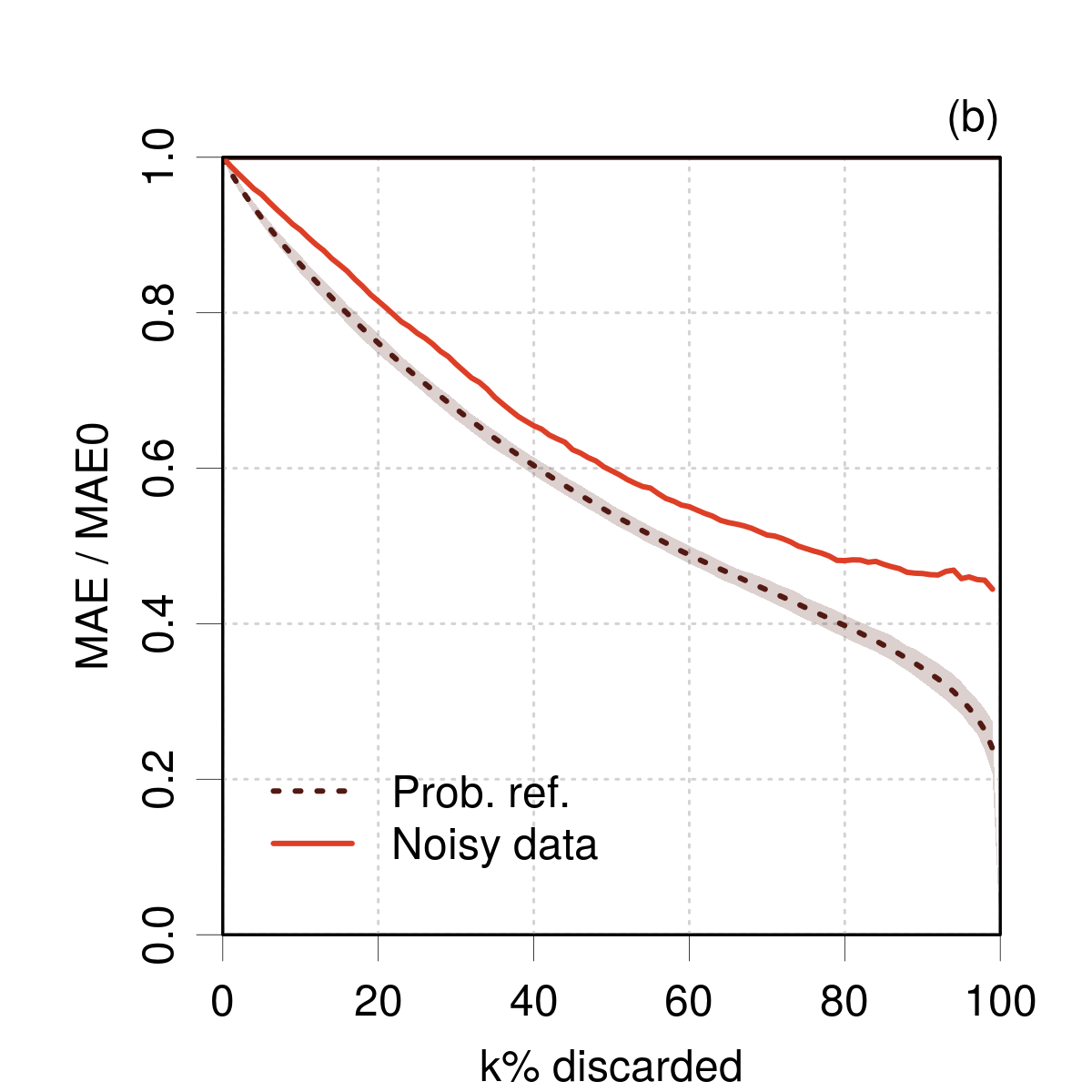
Confidence curves.
A confidence curve is established by estimating a statistic of error sets pruned from those points with uncertainties larger than a threshold.(Scalia2020, ) Technically, this is a ranking-based method, as the ordering of the data plays a determinant role.
For instance, if one defines a threshold by removing the % largest uncertainties (this applies also to expanded uncertainties), on gets a normalized confidence statistic as
| (20) |
where is an error statistic (typically the Mean Absolute Error). A continuously decreasing confidence curve reveals a desirable association between the larger errors and the larger uncertainties.
Usually, an oracle curve is plotted as reference,(Scalia2020, ) generated from an hypothetical dataset with perfect correlation between and [see Fig. 5(c)]. This reference is not realistic for the type of error distributions expected here. As an alternative, I proposed(Pernot2022c, ) to generate a reference curve from a pseudo-error set sampled from a distribution with mean 0 and standard deviation
| (21) |
The sampling is repeated to provide a stable mean reference curve and a confidence band (at the 95 % level). To avoid any ambiguity with the oracle, I refer to this curve as a probabilistic reference. The difference between oracle and probabilistic reference curves can be seen in Fig. 5(c). The effect of the choice of has been studied elsewhere.(Pernot2022c, ) To summarize, it does not practically affect the reference curve itself, but mostly the width of the confidence band. A normal distribution is a reasonable choice in absence of specific information about .
An essential point is that comparing the confidence curve to the oracle reference does not provide information about calibration nor tightness. In fact, any transformation of the uncertainties that does not affect their rank would result into exactly the same confidence curve. By contrast, pairing the confidence curve with the probabilistic reference can be considered as a proper variance-based tightness validation method. Interestingly, it provides two kinds of diagnostics: (1) a continuously decreasing confidence curve validates the use of the predictive uncertainties for active learning, regardless of calibration; and (2) a confidence curve in agreement with the probabilistic reference validates the tightness of the uncertainties. Its main weakness when compared to a local calibration method or to a reliability diagram is to depend explicitly (but weakly, as discussed above) on the choice of a probabilistic model. For the same reasons as discussed earlier, this tightness diagnostic has to be conditioned on a positive average calibration test.
V.2 Graphical representations
In practice, it is often more informative to plot the statistics and their confidence intervals than to perform the validation tests. Several plots have been proposed in the literature to check average calibration (e.g. calibration curves, PIT histograms) (Gneiting2014, ; Tran2020, ; Chung2021, ). They were tested in PER2022 and I found that they were of limited interest to the typical scenarios of computational chemistry UQ. They might nevertheless become handy in the cases where one has full probabilistic predictions,(Tran2020, ) but are not presented here as they do not provide tightness diagnostics.
V.2.1 Local coverage probability (LCP) and local range ratio (LRR) analyses
The local values of and can be plotted against the location of the group centers and compared to . The same plot can represent a series of values of interest (for instance, 0.5, 0.75 and 0.95). For a self-contained calibration/tightness diagnostic, the values for average calibration can also be displayed in the right margin of the plot.
Application to a 95% prediction interval (based on ) for the SYNT01 set is shown in Fig. 4(a), where one can see that the error bars based on for all groups along overlap the target probability, indicating a good tightness of prediction intervals. In the right margin, average calibration is also attested by the PICP value for the full dataset. These prediction intervals are therefore calibrated and tight.
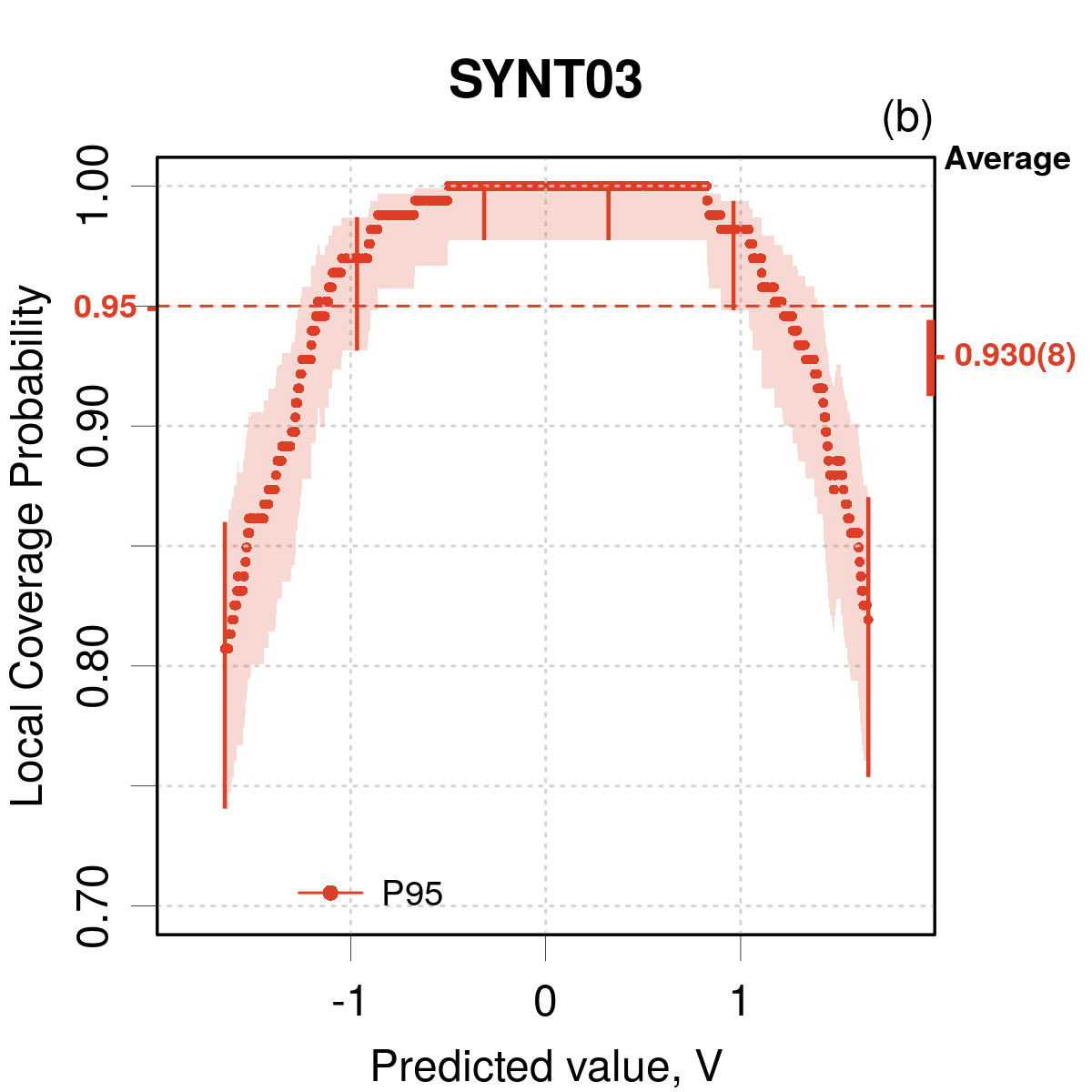
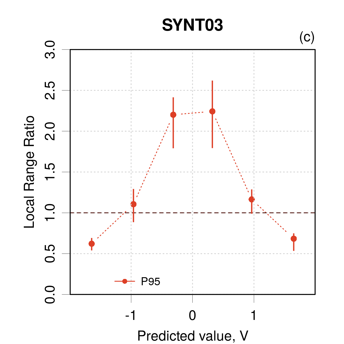

In contrast, the same analysis for the SYNT03 dataset [Fig. 4(b)] shows unambiguously a lack of tightness (average calibration is not optimal either considering the PICP value of 0.930(8)). It is clear from this graph that the constant uncertainty used for these data is only adapted for a few groups along . Moreover, the PICP values for the overestimated uncertainties saturate to 1.0, and we get no idea of the amplitude of the miscalibration from the LCP analysis. Plotting the local range ratio (LRR) statistic provides us with this information [Fig. 4(c)]. For the small uncertainties, underestimation is by a factor about 2.0, while for the large ones, the prediction interval’s width is overestimated by a factor about 2.3. Note that the LRR analysis did not use a sliding window because the excess computing time due to repeated bootstrapping does not contribute to the diagnostic. The computation overload is much less stringent for the LCP analysis, which does not use bootstrapping for confidence intervals estimation.
The same dataset can be used to illustrate how the statistics from a validation set enable to make calibrated predictions without ensuring tightness.(Levi2020, ) Expanded uncertainties are estimated from the empirical quantiles of the errors set, for and used to build uniform prediction intervals for all the points. The LCP analysis in Fig. 4(d) shows that calibration is good at all the levels (the PICP values in the right margin are consistent with their probability targets), but that tightness is not ensured at any level, as most LCP intervals do not overlap their target probability.
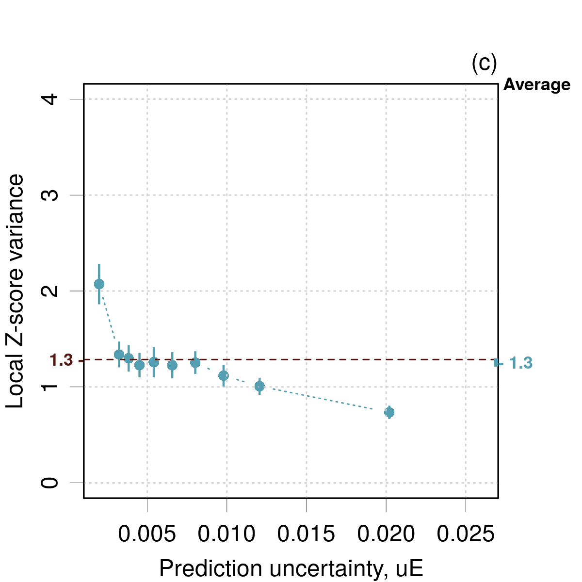
V.2.2 Local Z variance (LZV) analysis and reliability diagram
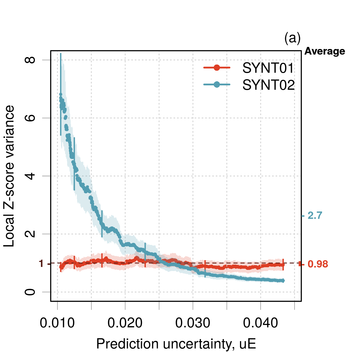
A similar representation can be used for the local validation of (LZV analysis). For the SYNT01 dataset [Fig. 5(a)], the test is fully consistent with , which is not the case for the SYNT02 dataset, for which varies between about 0.5 and 7, with an average value of 2.7. Note that for large validation sets, the use of a sliding window might present the same computation overload as for the LRR analysis, unless replacing the bootstrapping methods by the Cho method to estimate confidence intervals.
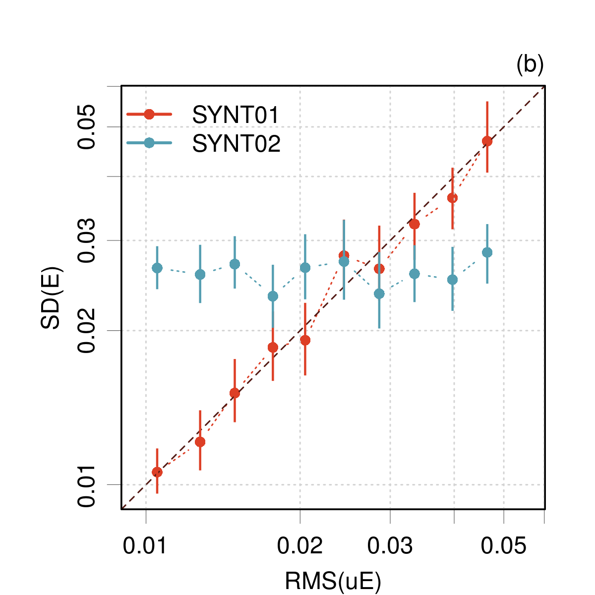
For comparison, the reliability diagram for SYNT01 and SYNT02 is presented in Fig. 5(b). The curve for SYNT01 follows closely the identity line, meaning that all levels of uncertainty describe correctly the dispersion of the corresponding errors (tightness). A contrario, the flat line for SYNT02 reveals the lack of consistency between errors and uncertainties. For the LZV analysis, the mismatch factor of the prediction uncertainty can be estimated locally by the square root of . With the reliability diagram, the same information can be obtained by taking the ratio between and .
For the same datasets, I plotted also the confidence curves [Fig. 5(c)]. As the curve for SYNT02 is non-decreasing, one can conclude readily to an absence of tightness. Comparing the confidence curve for SYNT01 to the oracle does not bring any information about calibration nor tightness. It seems to be far from the oracle, but still, the continuously decreasing curve is a positive feature. Comparison with the probabilistic reference let us unambiguously conclude that the errors match the probabilistic model relating them to uncertainties. Considering the good value of for this dataset, one might also conclude to a good tightness.
V.3 The problem of small probabilistic ensembles
It was assumed in Sect. III.2 that probabilistic predictions were made through distributions or prediction ensembles that were implicitly large enough to enable an accurate estimation of statistical summaries or empirical quantile functions used for validation. However, it is not uncommon to find applications where uncertainties are obtained as the standard deviation of small ensembles, typically with less than 10 values (see examples in Sect. VI). Estimation of quantiles from such small ensembles is not possible, barring recourse to intervals-based validation, and I would like to consider here how ranking- and variance-based validation methods perform in this context.
To illustrate the problem, let us consider a normal error distribution from which samples are drawn to estimate . Let us note the standard deviation of the ensembles. The distribution of for repeated sampling follows a scaled chi distribution with degrees of freedom
| (22) |
When considering a validation set one has therefore a variance source for entangled with the variance of , which makes the validation equation irrelevant. Kacker et al.(Kacker2010, ) formulated this in other terms by showing that the Birge ratio should not be used to estimate the statistical consistency of GUM(GUM, ) type A uncertainties. In fact, when uncertainty is estimated by the standard deviation of a small ensembles, the ratio of the mean error to the standard error is a t-score (or t-statistic)
| (23) |
In the case of a normal error distribution, has a Student’s-t distribution with degrees of freedom, and its variance is
| (24) |
When increases, the Student’s-t distribution converges to the standard normal, and one recovers .
We are thus left with two questions:
-
1.
For average calibration, how does Eq. 24 hold for non-normal distributions ? This point is studied in Appendix B and summarized here. Deviations from Eq. 24 for a large range of distribution shapes can mostly be neglected for . For smaller ensembles, one should allow for a wider range of values, that can be extracted from Fig. 12. For instance, for , values around 2, between 1.7 and 2.4, could be accepted.
-
2.
Which diagnostics can be used for tightness assessment ? This point is explored in Appendix C. The main conclusion is that all plots against (e.g. plots, LZV analysis vs. or reliability diagrams) are strongly perturbed by statistical noise and should not be used. A LZV analysis vs. is more useful in this context.
My recommendation for probabilistic predictions based on small ensembles () would thus be (1) to check average calibration through Eq. 24, possibly adapted for , and (2), conditional to average calibration, to check tightness through a LZV analysis vs. .
VI Examples
I present below several case studies based on datasets extracted from the computational chemistry literature. The first one, PRO2022,(Proppe2022, ) was already presented in PER2022 (under the PRO2021 tag). It is reconsidered here to show the interest and limits of the (,), LRR plots and confidence curves. In the same spirit, two other examples treated in PER2022 are also briefly treated together (PAN2015 and PAR2019). A recent dataset extracted from the ATOMIC-2um protocol(Bakowies2022, ) is introduced, along with two cases dealing with uncertainties extracted from small ensembles of predictions: LIN2021(Lin2021, ) from five repeats of a Free Energy Perturbation protocol and ZHE2022(Zheng2022, ) from an ensemble of eight neural networks (NN) predictions in a query by committee (QbC)(Smith2018, ) protocol.
VI.1 PRO2022444The data provided by Jonny Proppe were initially associated with a 2021 preprint by Proppe and Kircher (Proppe2021, ) and labeled PRO2021. For consistency, I now refer to the published version of the paper (Proppe2022, ) and label the data PRO2022.
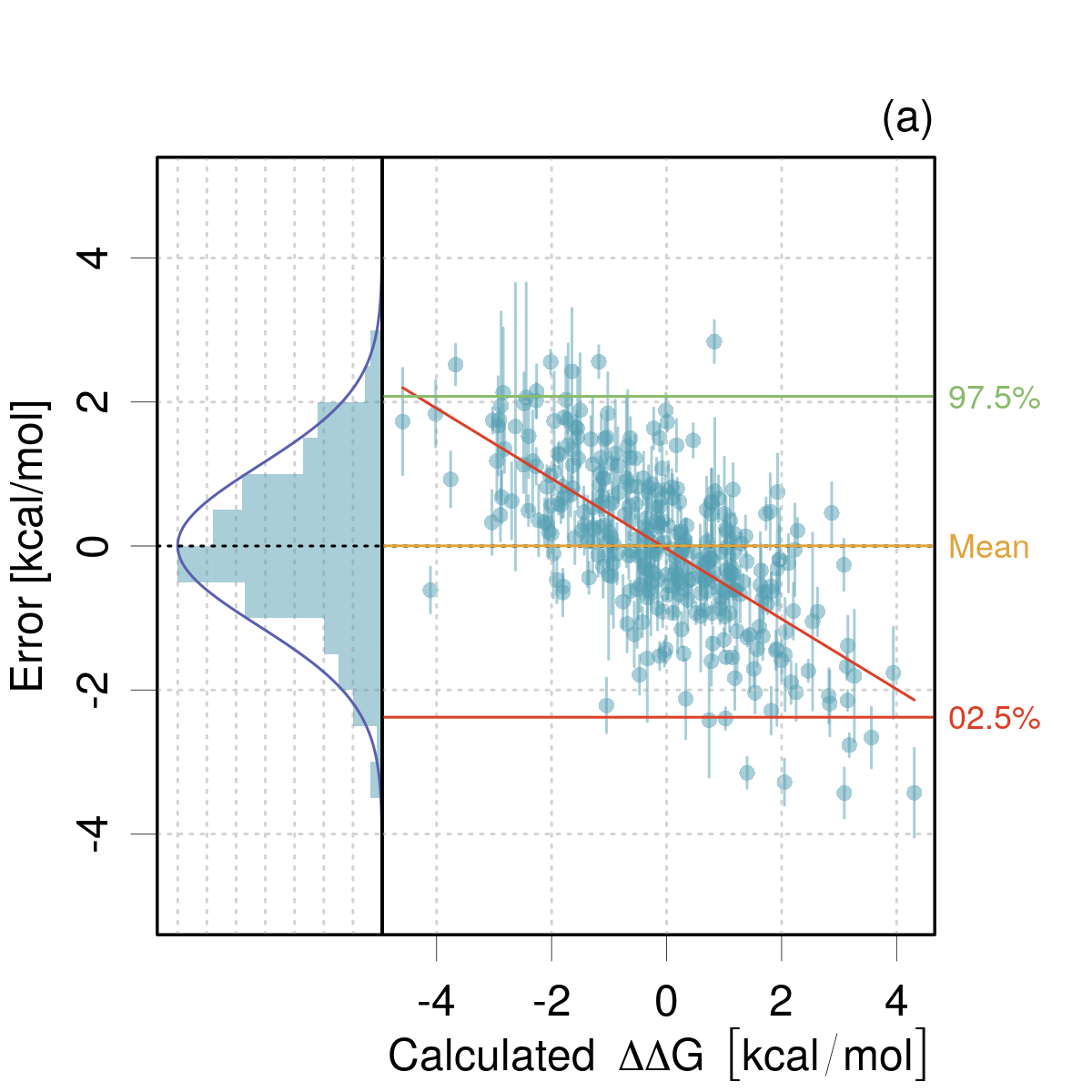
I revisit here the treatment I made of these data in PER2022(Pernot2022a, ). Proppe and Kircher(Proppe2022, ) compared two models to estimate a prediction uncertainty for the logarithm of reaction rates and provided expanded uncertainties for both models. The data are dimensionless. (,E) plots [Fig. 6(a,b)] show unambiguously that model is much better than model , in the sense that there is a better match between the scale of errors and uncertainties, notably for smaller uncertainties (below 0.2). However, one notices (as already done by Proppe and Kircher) that in both cases a single point is located outside of the interval, which suggests an overestimation of .
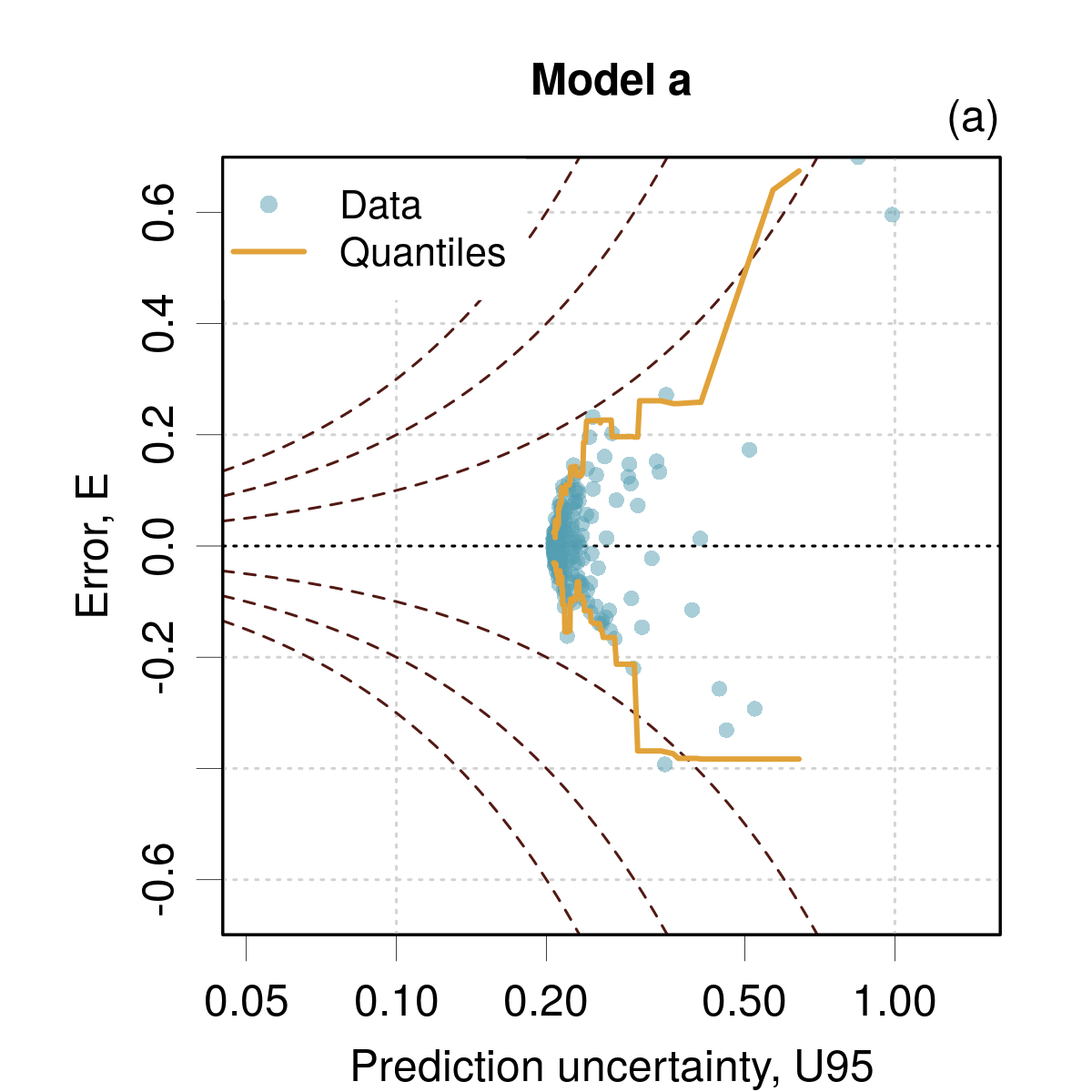
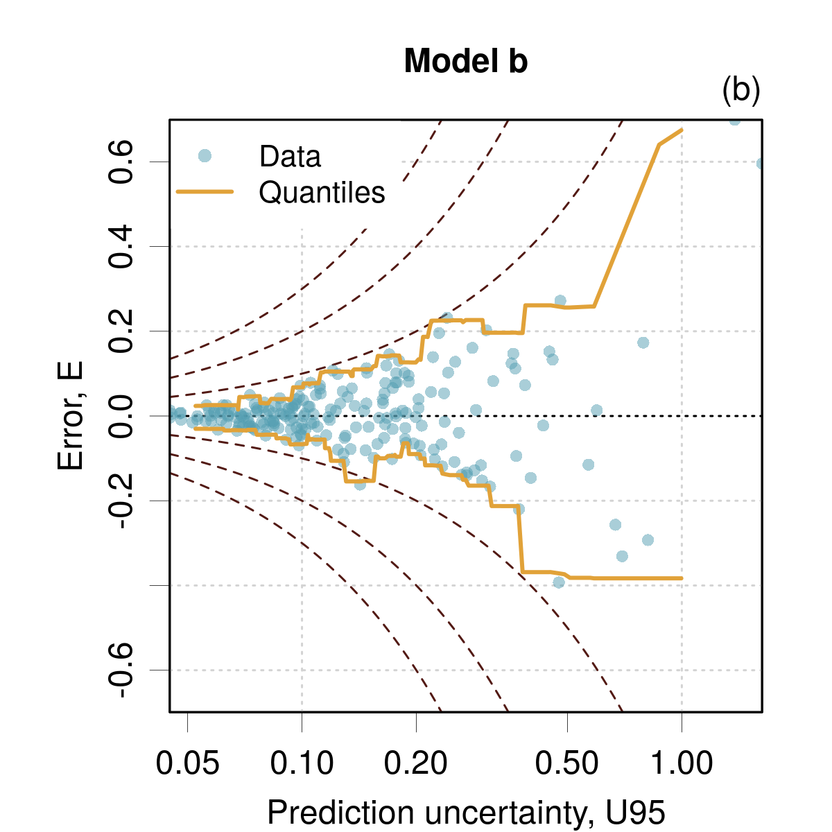
In fact, average calibration provides a PICP value of for both methods. The statistical uncertainty is too small for the confidence interval to include the target value (0.95). It is striking that, despite the difference observed in the (,E) plots, both models are identically calibrated, illustrating the shortcomings of considering average calibration without considering tightness.
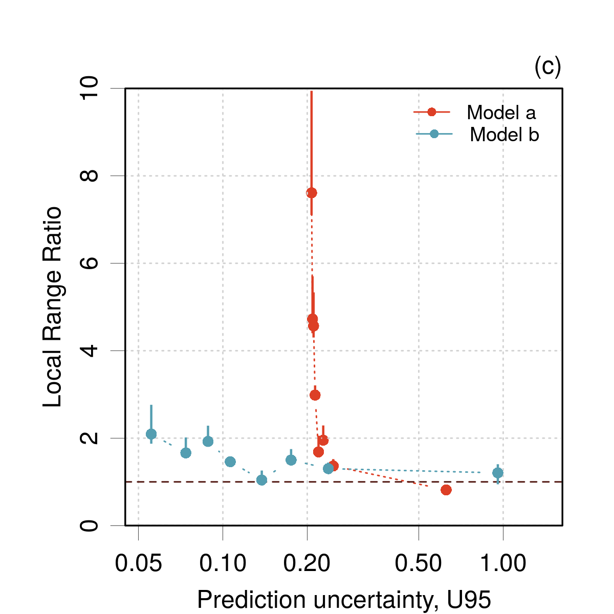
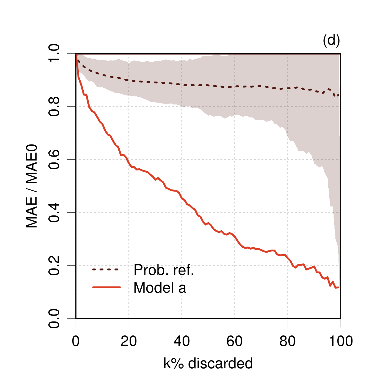
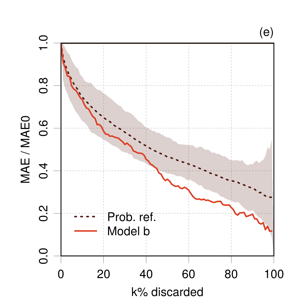
When PICP values are close to their upper limit, a LRR plot should be used to get a quantitative appreciation of the overestimation of (in PER2022, in the absence of the LRR analysis, a LZV analysis using was done). One can see on Fig. 6(c) that Model provides prediction intervals that can be up to eight times too wide, while this does not exceed a factor two for model .
Despite their considerable difference in calibration, both models have identical confidence curves [generated using , Fig. 6(d,e)], a reflection of the fact that both uncertainty sets have the same ranking (the Spearman (rank) correlation coefficient between both uncertainty sets is 1). However, the probabilistic reference curves enable to confirm the diagnostic that Model b is much closer to a good tightness than Model a. For Model b, it appears that the problem lies essentially in the small uncertainties. Despite the non-perfect calibration, one sees that both models provide uncertainties that would be suitable for active learning.
VI.2 BAK2022
Like its predecessor (ATOMIC(Bakowies2019, ; Bakowies2020, )), the ATOMIC-2um method(Bakowies2022, ) provides uncertainties on its predictions by a composite protocol. A set of 184 predictions has been compared to ATcT(Ruscic2014, ) reference values. The corresponding data (, , and ) have been collected from Table S20 of the reference article.
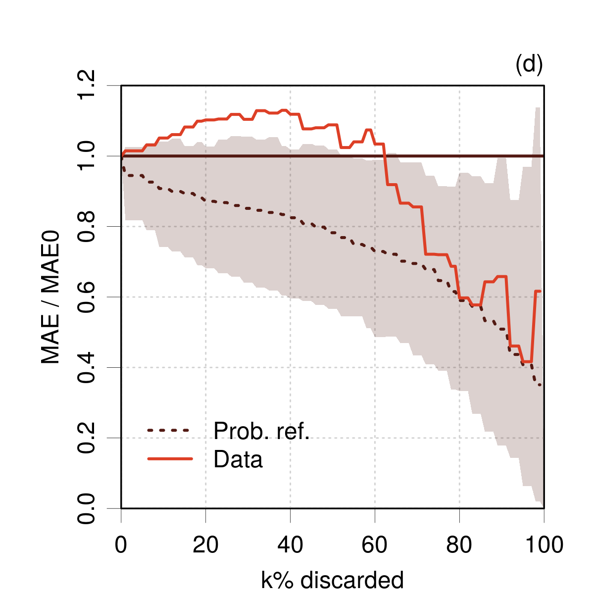
On the plot [Fig. 7(a)], the errors are well contained between the lines with a few outlying points. The seems however to be a slight bias of the errors towards the negative values that might compromise the hypothesis of symmetric prediction intervals. I checked that the correction of this bias does not improve the calibration/tightness results, so I worked with the original data.
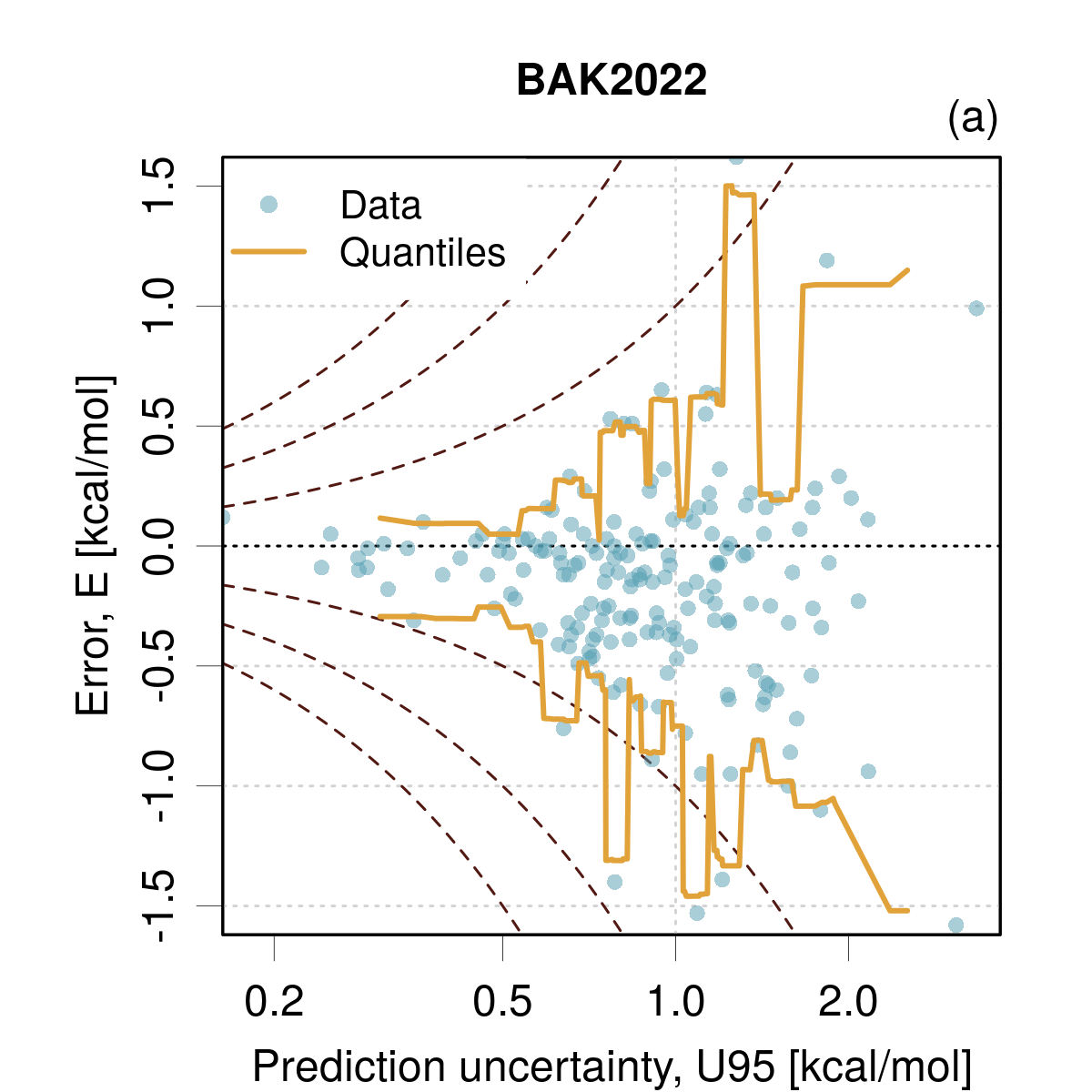
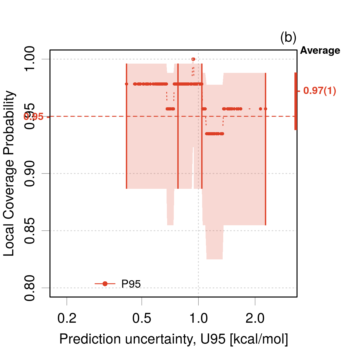
The uncertainties have been calibrated by Bakowies to target a 95% coverage in subsets of a large dataset (more than 1100 values), with an overall coverage of 97.2%.(Bakowies2022, ) From the more limited dataset used here, I get a compatible value of 0.97(1), which does not exclude the 0.95 target [Fig. 7(b)], although the LCP analysis shows a trend for overestimation of the small uncertainties. A confidence curve, built using confirms this diagnostic [Fig. 7(c)]. It shows a very good tightness, except for the bottom 25% of the uncertainties, where the curve drops and makes an excursion out of the probabilistic reference band.
Globally, these diagnostics confirm that the uncertainties estimated by the ATOMIC-2um protocol are globally and locally reliable, with a small trend to be conservative, notably for the smaller uncertainties (below ca. 0.7 kcal/mol). Note that in this range, the calculated uncertainties are in average four times larger than the reference uncertainties. It is therefore unlikely that the overestimation problem comes from the reference uncertainties.
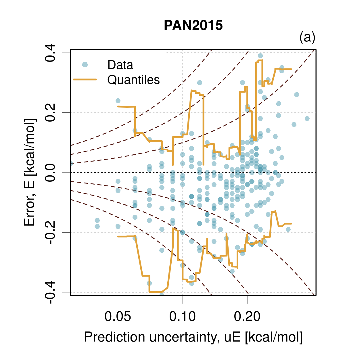
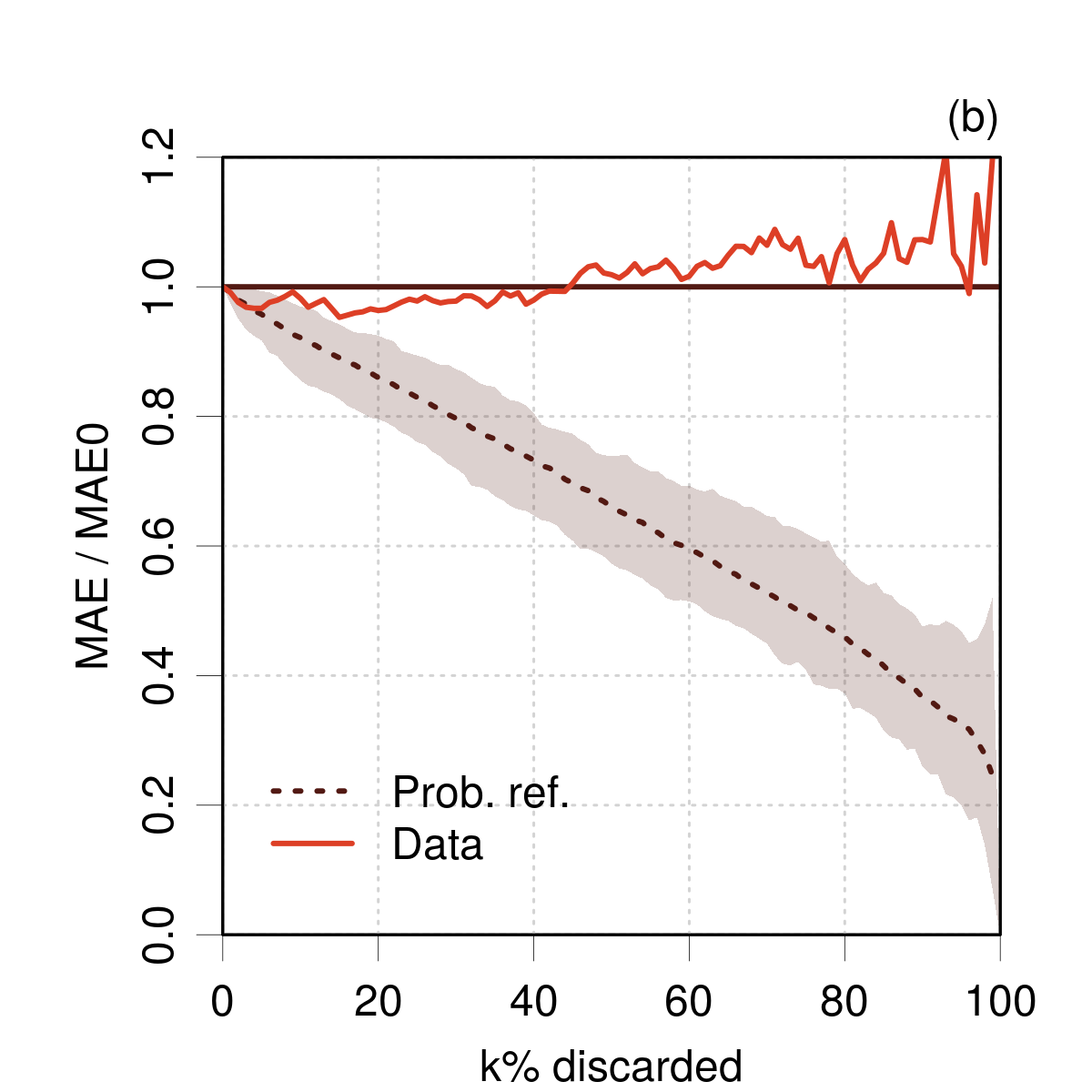
VI.3 PAN2015 and PAR2019
BEEF-based CC-UQ methods are calibrated through a parameters uncertainty inflation (PUI) scheme (Pernot2017, ; Pernot2017b, ) that implies strong functional constraints which play against their tightness. (Simm2016, ; Reiher2022, ) As the calibration is quantified by the mean prediction variance, there is no guarantee that the prediction uncertainty is reliable for any single prediction.
PAN2015.
This validation set of 257 formation heats and their standard uncertainties predicted by the mBEEF DFT has been extracted from a 2015 article by Pandey et al.(Pandey2015, ) I previously analyzed this dataset (Pernot2017b, ; Pernot2022a, ), showing an inconsistency between the prediction uncertainties and the errors amplitudes. A variance-based analysis has been performed in PER2022, showing a correct calibration with . However, the LZV analysis with respect to the prediction uncertainty revealed an absence of tightness, with values varying between 3 and 0.5. To complement this analysis, an plot and a confidence curve are reported in Fig. 8(a,b). The plot shows that uncertainties do not quantify correctly the dispersion of errors, but the most striking plot is certainly the confidence curve. As it is non-decreasing, it clearly reveals that errors and uncertainties are not statistically consistent. I find this representation to be the most revealing when compared to those presented in my earlier studies of this dataset.(Pernot2017b, ; Pernot2022a, )
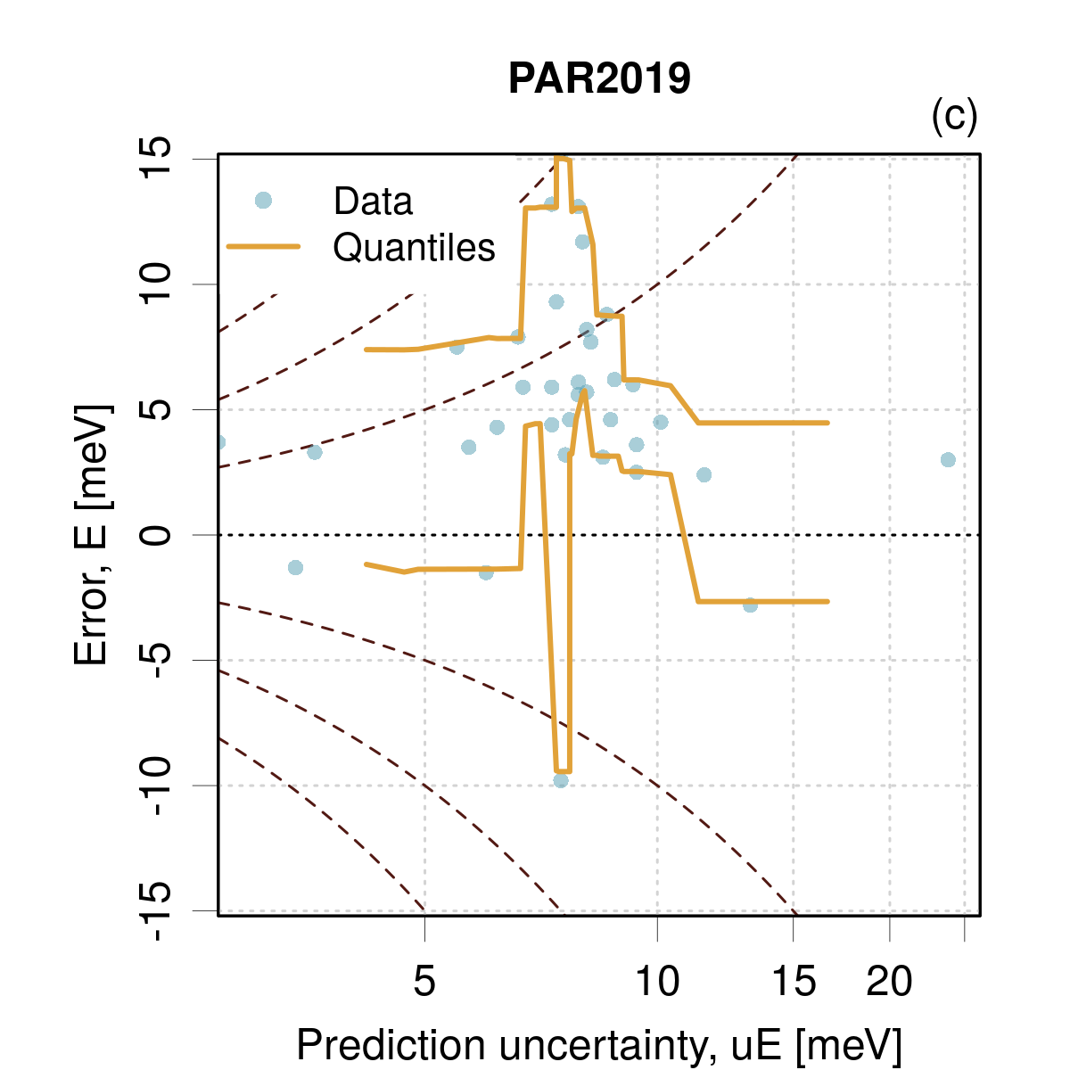
PAR2019.
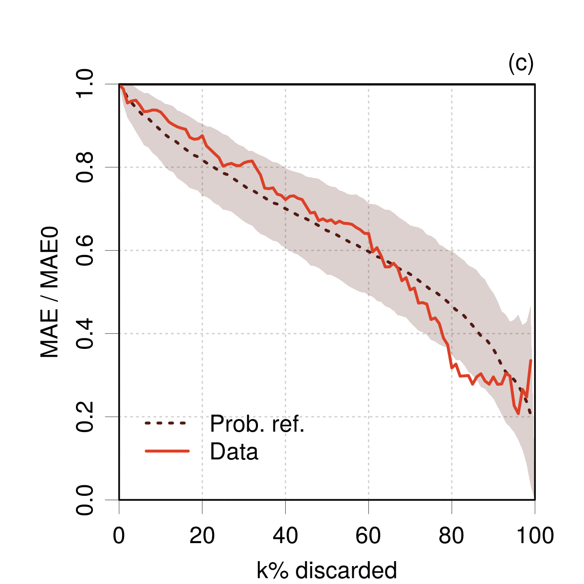
As another example of BEEF-generated uncertainties, I considered in PER2022 a small set of 35 harmonic vibrational frequencies issued from an article by Parks et al. (Parks2019, ). For this set, one has , a negative calibration test. The data are too sparse to attempt a LZV analysis. Fig. 8(c,d) reports the plot and confidence curve. Both plots enable to conclude to an absence of tightness, the confidence curve showing again an inconsistent ranking between absolute errors and uncertainties.
These examples clearly confirm that a method designed for average calibration on a learning set should not be expected to produce reliable prediction uncertainties.
VI.4 Small-ensemble predictions
VI.4.1 LIN2021
In a recent study on the prediction of binding free energies by the Free Energy Perturbation (FEP) protocol, Lin et al. (Lin2021, ) provided a set of data including reference experimental values, FEP values and FEP uncertainties for relative binding free energies (RBFE) and absolute binding free energies (ABFE). The RBFE dataset contains results for two versions of the FEP method, and I kept here the first one (Full FEP protocol) for which more data are provided (). Predicted values and uncertainties on the FEP procedures were produced by taking the mean and standard deviation of five repeats of the protocol (). To check the statistical consistency of the errors, one should therefore divide the reported standard deviations by .
The errors and their distribution are shown in Fig. 9(a). The errors have a quasi-normal distribution with a notable and unsuitable trend. The plot [Fig. 9(b)] shows that the errors seem unrelated to the uncertainties and that the uncertainties are too small to explain the dispersion of the errors. Confirming this point, the variance of t-scores is much too large ( vs. 2 for ). The confidence curve [Fig. 9(c), “Orig. data”] shows a very slow and shaky decrease, far above the reference curve, confirming a weak link between errors and uncertainties. The reported uncertainties for the FEP procedure should therefore not be interpreted nor used as prediction uncertainties. They should probably not be used either to identify predictions with large errors.
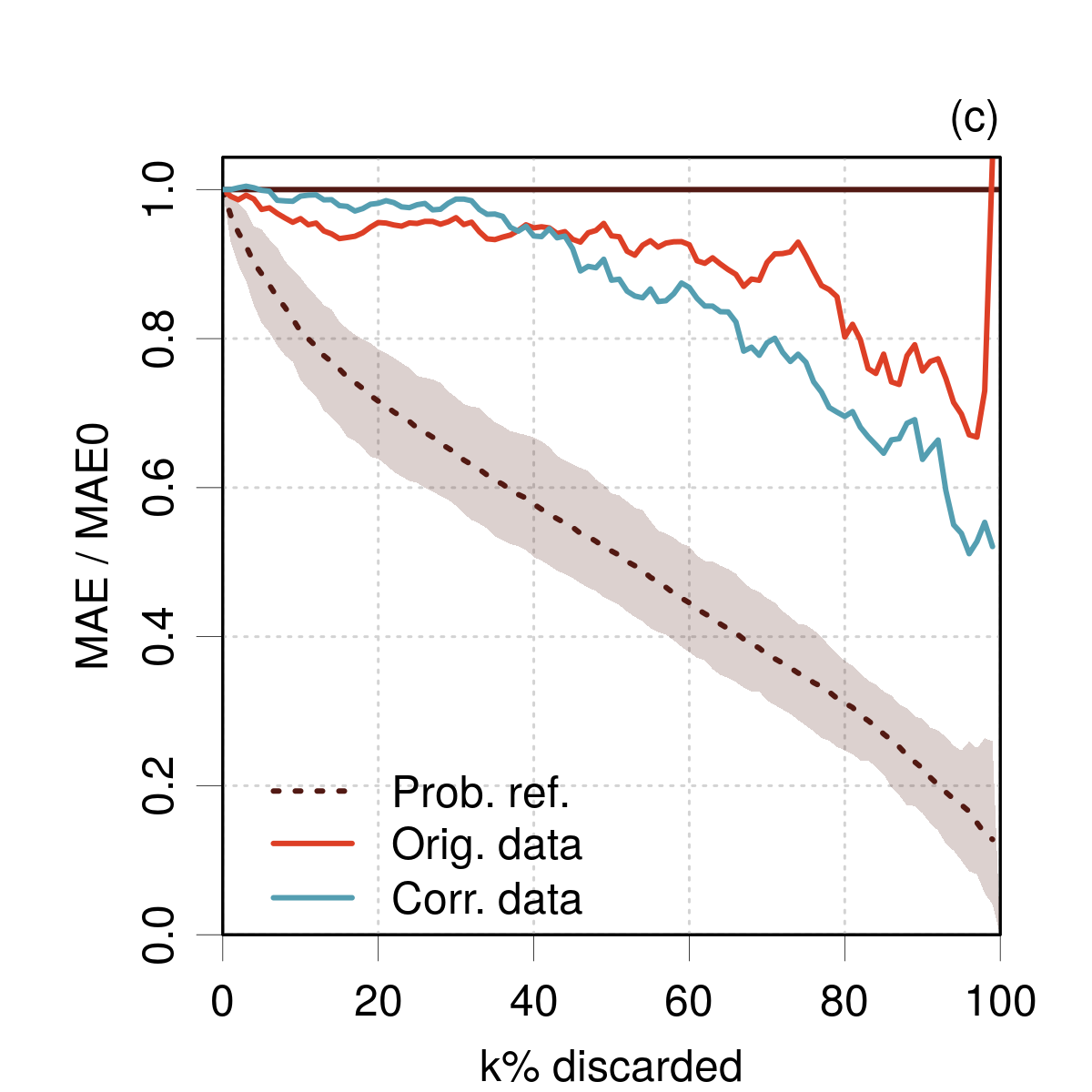
A linear trend correction, without modification of the uncertainties, improves notably the error distribution in terms of bias [Fig. 9(d)], but is insufficient to compensate for miscalibration [Fig. 9(e)]. The variance of the t-scores is reduced to , still far above the target value. The confidence curve is not improved either [as they share the same uncertainty set, both curves share the same probabilistic reference; Fig. 9(e)], and the LZV plots for the original and corrected data confirm the diagnostic.
The experimental uncertainty is reported to be about 0.4 kcal/mol for the kind of experimental data used as reference.(Wang2015c, ) Combining quadratically this value with the original uncertainties results in a significant but insufficient decrease of , to 6.1 () for the original data and 3.5 () for the corrected ones.
Model errors are not accounted for in the FEP UQ procedure, and one might conclude they have a non-negligible contribution to the error budget.
VI.4.2 ZHE2022
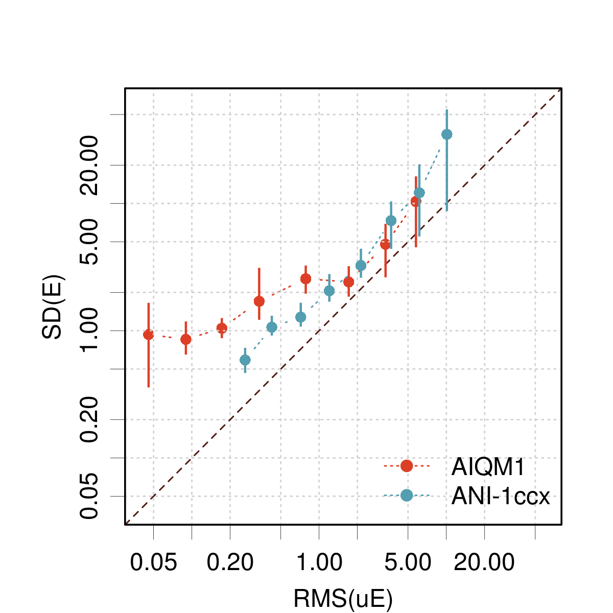
A recent article by Zheng et al. (Zheng2022, ) provides formation enthalpies and uncertainties for two data-driven methods, AIQM1 and ANI-1ccx. The uncertainties were obtained by a query by committee (QbC) strategy,(Smith2018, ) and taken as the standard deviation (SD) of the results for an ensemble of neural networks (NN). Zheng et al. consider that NN SDs provide uncertainty quantification on the methods predictions and used them to detect unreliable simulations, outliers and suspicious reference data. Two validation sets with were gathered from the source article for AIQM1 and ANI-1ccx, by aggregating data for and removing systems with missing values.
As in the QbC protocol the prediction value is taken as the mean of the NN predictions,(Smith2018, ) one should divide the reported standard deviations by for consistency. However, the authors used the standard deviation (which would be the uncertainty estimate for a single NN prediction) throughout their article, so I used it also to define . Furthermore, no information is provided about the uncertainty on the experimental data used as reference, and I ignore them in a first step.
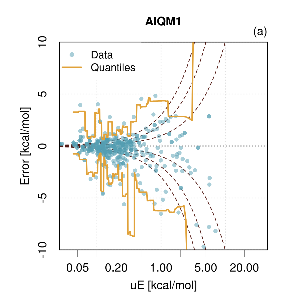
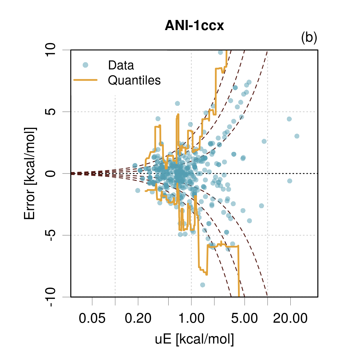
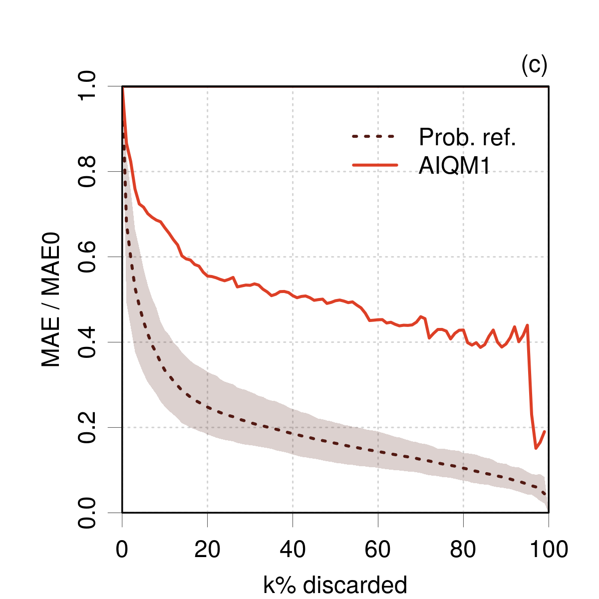
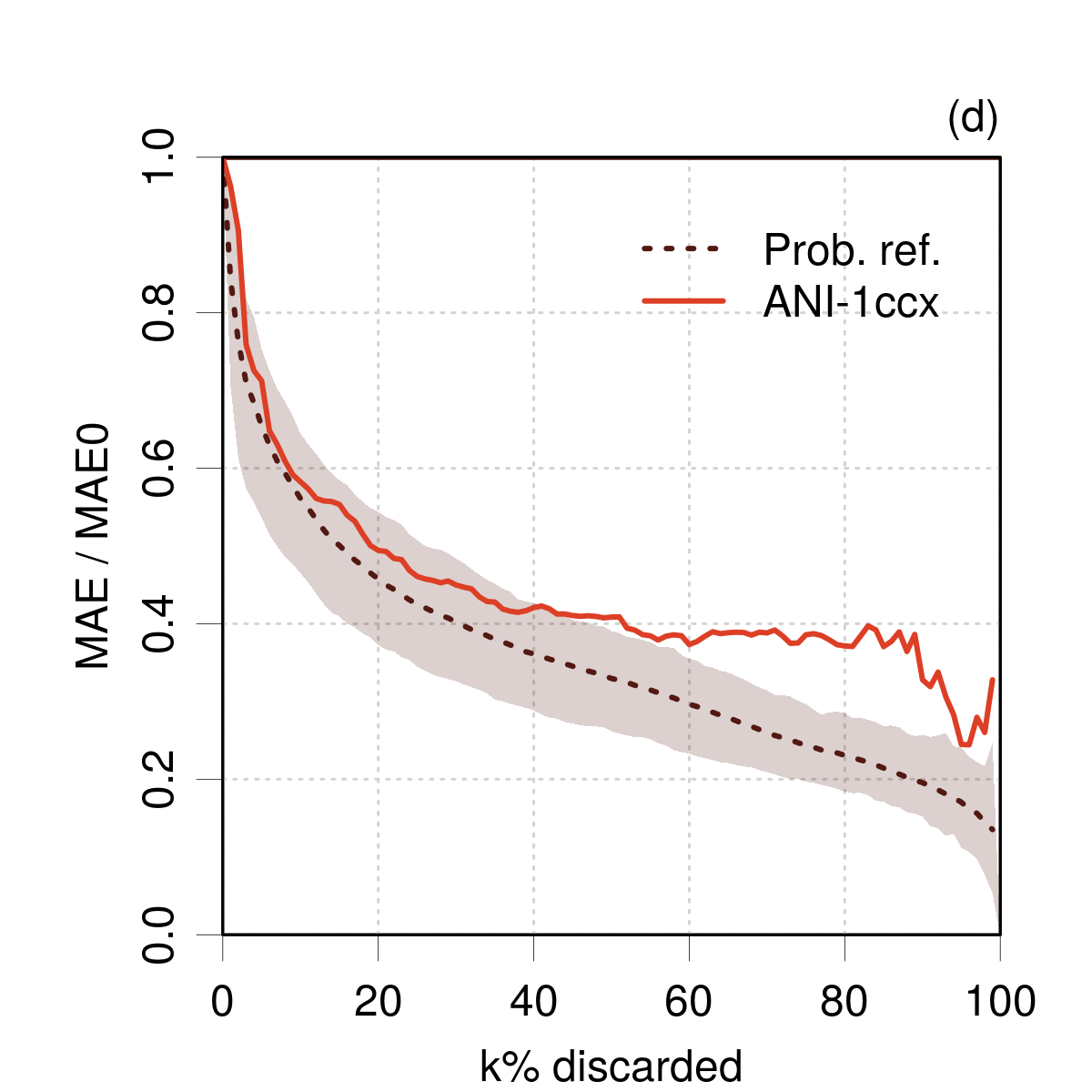
As a first diagnostic, one plots vs for both methods [Fig. 10(a,b)]. It is clear for the AIQM1 dataset that a large part of the uncertainties are too small to explain the amplitude of the errors. The consistency seems slightly better above 1 kcal/mol. One can safely reject calibration for this dataset, which is confirmed by the value of , to compare to the 1.4 target. Note that the scaling of the standard deviation by the factor would increase this value by a factor 8. The situation is somewhat better for the ANI-1ccx method [Fig. 10(b)], where the cumulative quantile curves follow grossly the guidelines. However, one has for this dataset, which leads to reject calibration.
As the score based on a linear regression without intercept used by the authors does not inform us on the correlations between and , I estimated the rank correlation coefficients for the CHNO subset and found 0.37 and 0.42 for AIQM1 and ANI-1ccx, respectively. These values are within the range reported by Tynes et al.(Tynes2021, ) for uncertainty datasets used in active learning (0.2 - 0.65). One might thus conclude that there is a rather strong relation between the QbC uncertainties and the prediction errors. This is assessed by the confidence curves [Fig. 10(c,d)]. Let us however note that these curves show a sharp decrease for the first fifth of the k axis and progressively switch to a slower decrease, or even a plateau for ANI-1ccx. This would mean that the consistency between errors and uncertainties is visible only for the 20% larger uncertainties. The departure of the confidence curves from the the probabilistic reference confirms the absence of calibration and tightness, with a better performance for ANI-1ccx.
Despite the absence of calibration, one might check the reliability of both sets on a reliability diagram [Fig. 10(d)]. Both sets have similar and slightly off reliability for the larger uncertainties (above 1 kcal/mol). Below this value, the ANI-1ccx performs better than AIQM1, with a nearly constant offset from the identity line. In contrast, the reliability curve for AIQM1 deviates from the identity line to reach a plateau, indicating a poor reliability of small uncertainties.
The median of the standard uncertainties derived666The ATcT provides expanded uncertainties. from the Active Thermochemical Tables (ATcT, ver. 1.112)(Ruscic2004, ) would be about 0.1 kcal/mol (the mean is about 0.17 kcal/mol). Adding quadratically a uniform contribution of 0.1 kcal/mol to the QbC uncertainties reduces to 29 and 4.1 for AIQM1 and ANI-1ccx, respectively. Experimental uncertainty alone is thus far from explaining the missing uncertainty and there should be a significant contribution of model errors. This is acknowledged by Zheng et al., who observed that some predictions with large errors have small QbC uncertainties.
This analysis confirms the findings of recent studies about the overconfidence of ensemble NN UQ protocols.(Tran2020, ; Scalia2020, ) It is clear from the present analysis that the QbC uncertainties cannot be considered as prediction uncertainties, mostly because they are not integrating model errors. However, as clearly demonstrated by Zheng et al. and observed on the confidence curves, they seem well fit for the purposes of active learning and outliers detection.
VII Available software
Except for simple graphical diagnostics presented in Sect. IV, extensive coding might be required to implement the CS/CT validation methods. To my knowledge, three toolboxes are freely available that implement some of these methods.
-
•
Uncertainty Toolbox. “A python toolbox for predictive uncertainty quantification, calibration, metrics, and visualizations”.(Chung2021, ) The toolbox focuses on regression tasks in ML-UQ. It implements, among other, calibration and sharpness statistics, adversarial group calibration and some re-calibration methods.
-
•
scoringutils “The scoringutils package provides a collection of metrics and proper scoring rules and aims to make it simple to score probabilistic forecasts against the true observed values.” Issued in 2022, this R package deals with predictive probability distributions represented as sample or parametric distributions.(Jordan2019, ; Bosse2022, )
-
•
ErrViewLib. Coded in R,(RTeam2019, ) the package implements functions for simple graphical checks (plotEvsPU) and calibration/tightness analysis (plotLCP, plotLRR, plotLZV, plotRelDiag and plotConfidence). It is not ML oriented and does not presently treat prediction ensembles. All the plots of the present study have been generated with ErrViewLib-v1.5d (https://github.com/ppernot/ErrViewLib/releases/tag/v1.5d), also available at Zenodo (https://doi.org/10.5281/zenodo.6783307). Alg. 1 presents a skeletal example to generate a () plot and a LCP analysis for an heteroscedastic synthetic dataset. The UncVal graphical interface to explore the main UQ validation methods provided by ErrViewLib is also available on GitHub (https://github.com/ppernot/UncVal), either as source code or as a Docker container.
library(ErrViewLib)N = 1000s2 = rchisq(N, df = 4) # Random varianceuE = 0.01 * sqrt(s2/mean(s2)) # Re-scale uncertaintyE = rnorm(N, mean=0, sd=uE) # Generate errorsErrViewLib::plotEvsPU(uE, E)U95 = 1.96*uE # U95 for normal lawErrViewLib::plotLCP(E, U95, ordX = U95, prob = 0.95, ylim = c(0.5,1))Algorithm 1 Example of R script using ErrViewLib.
VIII Discussion and conclusion
This article presents a comprehensive panel of simple and more complex graphical and statistical methods to test the calibration and tightness of probabilistic predictions. Tightness has been introduced as a concept to evaluate the small-scale reliability of probabilistic predictions. As for sharpness, its use is conditional to average calibration. The full validation of the reliability of probabilistic predictions requires thus the estimation of (average) calibration and tightness.
The tool set presented in PER2022 for intervals- and variance-based validation has been completed by easy to implement graphical checks and by ranking-based methods (correlation coefficients, confidence curves) used in machine learning(Scalia2020, ). A summary of the applicability and validation capacity of all the methods is presented in Table 1.
| Diagnostic | Applicability | Validation | |||||||
|---|---|---|---|---|---|---|---|---|---|
| Homosc. | Heterosc. | Calibrat. | Tightness | ||||||
| Average | |||||||||
| PIT hist. | |||||||||
| Calib. curve | |||||||||
| PICP | |||||||||
| Var() | |||||||||
| Cor(,) | ∗ | ||||||||
| Local | |||||||||
| LCP/LRR | † | ||||||||
| LZV | † | ||||||||
| Reliab. diag. | † | ||||||||
| Confid. curve (oracle) | ∗ | ||||||||
| Confid. curve (prob.) | † | ||||||||
We have seen that the ranking-based methods are not able to give a positive validation diagnostic, but they might be used to ascertain a negative tightness diagnostic. Note that ranking-based methods find their utility in active learning, where the main purpose of an uncertainty is to identify cases susceptible of large errors. From a set of average-calibrated methods, on should prefer the one with the best sharpness or confidence curve, but we have no guarantee that it might have a good tightness. Besides, ranking-based methods cannot be used for homoscedastic datasets (i.e. validation sets for which all predictions have the same uncertainty). We are thus left with intervals- and variance-based validation methods, the choice of which is guided by available information.
When predictions are represented by analytical distributions or large ensembles, all methods are available. Either for calibration or tightness validation, testing for the adequacy of a set of intervals with different coverage probabilities will be more demanding than testing for variance, as the latter is less dependent on the shape of the distribution. However, unless the distribution’s shape is very far from normal, e.g. with a strong asymmetry, variance-based methods should be adequate.
In many instances, the literature about computational chemistry uncertainty quantification reports only statistical summaries, i.e. standard uncertainties or expanded uncertainties at the 95 % level. In such cases, the choice of validation method is imposed: standard uncertainties should be handled by variance-based methods and expanded uncertainties by intervals-based methods. Of course, in cases where expanded uncertainties were derived from standard uncertainties by a known expansion factor, inverse transformation to standard uncertainties can give access to variance-based methods.
In the proposed framework, calibration is validated on the full validation set, using prediction intervals coverage probabilities (PICP) for the intervals-based approach and the variance of scaled errors or z-scores () for the variance-based approach. Tightness validation is based the same tools, but applied to subsets or groups of the validation set to assess local or small-scale reliability, leading to LCP analysis for the intervals-based approach and to LZV analysis for the variance-based approach. The groups can be designed according to any relevant criteria, but using the predicted value and the prediction uncertainty are two interesting alternatives. I have shown that the latter case is closely linked to the reliability diagrams introduced by Levi et al.(Levi2020, ). Note that by using a new probabilistic reference, confidence curves have been promoted from a ranking-based to a variance-based validation method for tightness. Reliability diagrams and confidence curves can only be used for heteroscedastic datasets.
A special care has to be taken for those cases where uncertainty is estimated as the standard deviation of a small ensemble (). In such cases, the scaled errors are not z-scores, but t-scores, for which the theoretical variance used for validation is (for normal predictive distributions) instead of 1 for z-scores. With this caveat in mind, it is possible to validate calibration, but we have seen that tightness is very sensitive to the statistical noise characteristic of small ensembles. In particular, the LZV approach with groups based on the prediction uncertainty, or the reliability diagrams, will reject tightness. In this case, using the predicted value as a grouping feature for the LZV analysis is a better alternative.
The tools presented in this study are of interest primarily to CC-UQ researchers in order to validate their methods to generate prediction uncertainties, but the most simple of them, such as the plot, can easily be applied by end users curious to evaluate and gain confidence in uncertainties they might want to publish or reuse. UQ outputs failing to satisfy these validation tests should be used with caution and not over-interpreted. They should not be used to infer probability intervals for the true value of a property, as would be expected in the Virtual Measurements framework.(Irikura2004, ) All the examples taken from the literature, as well as those presented in PER2022 show that designing reliable prediction uncertainties is a very demanding process, which leaves ample room for future developments in CC-UQ.
Data availability statement
The data and codes that enable to reproduce the figures of this study are openly available at the following URL: https://github.com/ppernot/2022_Tightness, or in Zenodo at https://doi.org/10.5281/zenodo.7059776.
Acknowledgments
I would like to thank Andreas Savin for enlightening and constructive discussions, Jonny Proppe for providing the PRO2022 dataset, Pavlo Dral for helpful comments on a former version of my analysis of the ZHE2022 dataset, and Matthew Evans for pointing out the Uncertainty Toolbox.
References
- (1) T. Weymuth and M. Reiher. Heuristics and uncertainty quantification in rational and inverse compound and catalyst design. In Reference Module in Chemistry, Molecular Sciences and Chemical Engineering. Elsevier, 2022.
- (2) J. P. Janet, C. Duan, T. Yang, A. Nandy, and H. J. Kulik. A quantitative uncertainty metric controls error in neural network-driven chemical discovery. Chem. Sci., 10:7913–7922, 2019.
- (3) F. Musil, M. J. Willatt, M. A. Langovoy, and M. Ceriotti. Fast and accurate uncertainty estimation in chemical machine learning. J. Chem. Theory Comput., 15:906–915, 2019.
- (4) G. Scalia, C. A. Grambow, B. Pernici, Y.-P. Li, and W. H. Green. Evaluating scalable uncertainty estimation methods for deep learning-based molecular property prediction. J. Chem. Inf. Model., 60:2697–2717, 2020.
- (5) K. Tran, W. Neiswanger, J. Yoon, Q. Zhang, E. Xing, and Z. W. Ulissi. Methods for comparing uncertainty quantifications for material property predictions. Mach. Learn.: Sci. Technol., 1:025006, 2020.
- (6) D. Wang, J. Yu, L. Chen, X. Li, H. Jiang, K. Chen, M. Zheng, and X. Luo. A hybrid framework for improving uncertainty quantification in deep learning-based QSAR regression modeling. J. Cheminf., 13:69, 2021.
- (7) N. Zhan and J. R. Kitchin. Uncertainty quantification in machine learning and nonlinear least squares regression models. AIChE J., 68:e17516, 2021.
- (8) G. Imbalzano, Y. Zhuang, V. Kapil, K. Rossi, E. A. Engel, F. Grasselli, and M. Ceriotti. Uncertainty estimation for molecular dynamics and sampling. J. Chem. Phys., 154:074102, 2021.
- (9) J. Busk, P. B. Jørgensen, A. Bhowmik, M. N. Schmidt, O. Winther, and T. Vegge. Calibrated uncertainty for molecular property prediction using ensembles of message passing neural networks. Mach. Learn.: Sci. Technol., 3:015012, 2022.
- (10) Y. Hu, J. Musielewicz, Z. Ulissi, and A. J. Medford. Robust and scalable uncertainty estimation with conformal prediction for machine-learned interatomic potentials. arXiv:2208.08337, August 2022.
- (11) P. Pernot, B. Civalleri, D. Presti, and A. Savin. Prediction uncertainty of density functional approximations for properties of crystals with cubic symmetry. J. Phys. Chem. A, 119:5288–5304, 2015.
- (12) S. De Waele, K. Lejaeghere, M. Sluydts, and S. Cottenier. Error estimates for density-functional theory predictions of surface energy and work function. Phys. Rev. B, 94:235418, 2016.
- (13) J. Proppe, T. Husch, G. N. Simm, and M. Reiher. Uncertainty quantification for quantum chemical models of complex reaction networks. Faraday Discuss., 195:497–520, 2016.
- (14) P. Pernot and F. Cailliez. A critical review of statistical calibration/prediction models handling data inconsistency and model inadequacy. AIChE J., 63:4642–4665, 2017.
- (15) J. Proppe and M. Reiher. Reliable estimation of prediction uncertainty for physicochemical property models. J. Chem. Theory Comput., 13:3297–3317, 2017.
- (16) P. Pernot. The parameter uncertainty inflation fallacy. J. Chem. Phys., 147:104102, 2017.
- (17) J. Proppe, S. Gugler, and M. Reiher. Gaussian process-based refinement of dispersion corrections. J. Chem. Theory Comput., 15:6046–6060, 2019.
- (18) K. Lejaeghere. The uncertainty pyramid for electronic-structure methods. In Y. Wang and D. L. McDowell, editors, Uncertainty Quantification in Multiscale Materials Modeling, Elsevier Series in Mechanics of Advanced Materials, pages 41 – 76. Woodhead Publishing, 2020.
- (19) J. Proppe and J. Kircher. Uncertainty quantification of reactivity scales. ChemPhysChem, 23:e202200061, 2022.
- (20) P. Pernot. The long road to calibrated prediction uncertainty in computational chemistry. J. Chem. Phys., 156:114109, 2022.
- (21) M. Reiher. Molecule-specific uncertainty quantification in quantum chemical studies. Isr. J. Chem., 62(1-2):e202100101, 2022.
- (22) T. Gneiting and M. Katzfuss. Probabilistic forecasting. Annu. Rev. Stat. Appl., 1:125–151, 2014.
- (23) V. Kuleshov, N. Fenner, and S. Ermon. Accurate uncertainties for deep learning using calibrated regression. In J. Dy and A. Krause, editors, Proceedings of the 35th International Conference on Machine Learning, volume 80 of Proceedings of Machine Learning Research, pages 2796–2804. PMLR, 10–15 Jul 2018. URL: https://proceedings.mlr.press/v80/kuleshov18a.html.
- (24) D. Levi, L. Gispan, N. Giladi, and E. Fetaya. Evaluating and calibrating uncertainty prediction in regression tasks. Sensors, 22:5540, 2022.
- (25) F. Küppers, J. Schneider, and A. Haselhoff. Parametric and multivariate uncertainty calibration for regression and object detection. arXiv:2207.01242, 2022.
- (26) B. Ruscic. Uncertainty quantification in thermochemistry, benchmarking electronic structure computations, and active thermochemical tables. Int. J. Quantum Chem., 114:1097–1101, 2014.
- (27) P. Pernot and A. Savin. Probabilistic performance estimators for computational chemistry methods: the empirical cumulative distribution function of absolute errors. J. Chem. Phys., 148:241707, 2018.
- (28) P. Pernot, B. Huang, and A. Savin. Impact of non-normal error distributions on the benchmarking and ranking of Quantum Machine Learning models. Mach. Learn.: Sci. Technol., 1:035011, 2020.
- (29) P. Pernot and A. Savin. Using the Gini coefficient to characterize the shape of computational chemistry error distributions. Theor. Chem. Acc., 140:24, 2021.
- (30) Y. Chung, I. Char, H. Guo, J. Schneider, and W. Neiswanger. Uncertainty toolbox: an open-source library for assessing, visualizing, and improving uncertainty quantification. arXiv, 2021. arXiv:2109.10254.
- (31) U. Hébert-Johnson, M. P. Kim, O. Reingold, and G. N. Rothblum. Calibration for the (computationally-identifiable) masses. arXiv, 2017. arXiv:1711.08513.
- (32) J. S. Smith, B. Nebgen, N. Lubbers, O. Isayev, and A. E. Roitberg. Less is more: Sampling chemical space with active learning. J. Chem. Phys., 148:241733, 2018.
- (33) P. Zheng, W. Yang, W. Wu, O. Isayev, and P. O. Dral. Toward chemical accuracy in predicting enthalpies of formation with general-purpose data-driven methods. J. Phys. Chem. Lett., 13:3479–3491, 2022.
- (34) M. Tynes, W. Gao, D. J. Burrill, E. R. Batista, D. Perez, P. Yang, and N. Lubbers. Pairwise difference regression: A machine learning meta-algorithm for improved prediction and uncertainty quantification in chemical search. J. Chem. Inf. Model., 61:3846–3857, 2021. PMID: 34347460.
- (35) BIPM, IEC, IFCC, ILAC, ISO, IUPAC, IUPAP, and OIML. Evaluation of measurement data - Guide to the expression of uncertainty in measurement (GUM). Technical Report 100:2008, Joint Committee for Guides in Metrology, JCGM, 2008. URL: http://www.bipm.org/utils/common/documents/jcgm/JCGM_100_2008_F.pdf.
- (36) Recently introduced,(Cox2022, ) characteristic uncertainty is estimated by . This proposition covers the gap between and in terms of information needed for prediction interval design.
- (37) Y. Lai, Y. Shi, Y. Han, Y. Shao, M. Qi, and B. Li. Exploring uncertainty in regression neural networks for construction of prediction intervals. Neurocomputing, 481:249–257, 2022.
- (38) Y. Chung, W. Neiswanger, I. Char, and J. Schneider. Beyond pinball loss: Quantile methods for calibrated uncertainty quantification. arXiv:2011.09588, 2020.
- (39) R. R. Wilcox and D. M. Erceg-Hurn. Comparing two dependent groups via quantiles. J. App. Stat., 39:2655–2664, 2012.
- (40) R. R. Wilcox and G. A. Rousselet. A guide to robust statistical methods in neuroscience. Curr. Prot. Neuroscience, 82:8.42.1–8.42.30, 2018.
- (41) B. Efron. Bootstrap Methods: Another Look at the Jackknife. Ann. Stat., 7:1–26, January 1979.
- (42) B. Efron and R. Tibshirani. Statistical data analysis in the computer age. Science, 253:390–395, 1991.
- (43) C. Tomani, S. Gruber, M. Erdem, D. Cremers, and F. Buettner. Post-hoc uncertainty calibration for domain drift scenarios. In 2021 IEEE/CVF Conference on Computer Vision and Pattern Recognition (CVPR), pages 10119–10127, Los Alamitos, CA, USA, jun 2021. IEEE Computer Society.
- (44) Note that this definition differs from the one in the calibration/sharpness literature (see e.g. Kuleshov et al.(Kuleshov2018, )) by my consideration of reference data uncertainty in the prediction interval.
- (45) S. E. Vollset. Confidence intervals for a binomial proportion. Stat Med, 12:809–824, 1993.
- (46) R Core Team. R: A Language and Environment for Statistical Computing. R Foundation for Statistical Computing, Vienna, Austria, 2019. URL: http://www.R-project.org/.
- (47) A. Agresti and B. A. Coull. Approximate is better than ’exact’ for interval estimation of binomial proportions. Am. Stat., 52:119–126, 1998.
- (48) C. J. Clopper and E. S. Pearson. The use of confidence or fiducial limits illustrated in the case of the binomial. Biometrika, 26:404–413, 1934.
- (49) R. G. Newcombe. Two-sided confidence intervals for the single proportion: comparison of seven methods. Stat. Med., 17:857–872, 1998.
- (50) R. T. Birge. The calculation of errors by the method of least squares. Phys. Rev., 40:207–227, 1932.
- (51) R. N. Kacker, R. Kessel, and K.-D. Sommer. Assessing differences between results determined according to the guide to the expression of uncertainty in measurement. J. Res. Nat. Inst. Stand. Technol., 115(6):453, 2010.
- (52) O. Bodnar and C. Elster. On the adjustment of inconsistent data using the Birge ratio. Metrologia, 51:516–521, 2014.
- (53) T. J. DiCiccio and B. Efron. Bootstrap confidence intervals. Statist. Sci., 11:189–212, 1996. URL: https://www.jstor.org/stable/2246110.
- (54) E. Cho, M. J. Cho, and J. Eltinge. The variance of sample variance from a finite population. Int. J. Pure Appl. Math., 21:387–394, 2005. URL: http://www.ijpam.eu/contents/2005-21-3/10/10.pdf.
- (55) Not to be confounded with the Birge ratio, also noted (Appendix\tmspace+.1667emA).
- (56) F. Pedregosa, G. Varoquaux, A. Gramfort, V. Michel, B. Thirion, O. Grisel, M. Blondel, P. Prettenhofer, R. Weiss, V. Dubourg, J. Vanderplas, A. Passos, D. Cournapeau, M. Brucher, M. Perrot, and E. Duchesnay. Scikit-learn: Machine learning in Python. J. Mach. Learn. Res., 12:2825–2830, 2011. URL: https://www.jmlr.org/papers/v12/pedregosa11a.html.
- (57) P. Pernot. Confidence curves for UQ validation: probabilistic reference vs. oracle. arXiv:2206.15272, 2022.
- (58) D. Bakowies. Atomic-2 protocol for thermochemistry. J. Chem. Theory Comput., 18:4142–4163, 2022.
- (59) Z. Lin, J. Zou, S. Liu, C. Peng, Z. Li, X. Wan, D. Fang, J. Yin, G. Gobbo, Y. Chen, J. Ma, S. Wen, P. Zhang, and M. Yang. A Cloud Computing Platform for Scalable Relative and Absolute Binding Free Energy Predictions: New Opportunities and Challenges for Drug Discovery. J. Chem. Inf. Model., 61:2720–2732, 2021.
- (60) The data provided by Jonny Proppe were initially associated with a 2021 preprint by Proppe and Kircher (Proppe2021, ) and labeled PRO2021. For consistency, I now refer to the published version of the paper (Proppe2022, ) and label the data PRO2022.
- (61) D. Bakowies. Estimating systematic error and uncertainty in ab initio thermochemistry. I. Atomization energies of hydrocarbons in the ATOMIC(hc) protocol. J. Chem. Theory Comput., 15:5230–5251, 2019.
- (62) D. Bakowies. Estimating systematic error and uncertainty in ab initio thermochemistry: II. ATOMIC(hc) enthalpies of formation for a large set of hydrocarbons. J. Chem. Theory Comput., 16:399–426, 2020.
- (63) G. N. Simm and M. Reiher. Systematic Error Estimation for Chemical Reaction Energies. J. Chem. Theory Comput., 12:2762–2773, 2016.
- (64) M. Pandey and K. W. Jacobsen. Heats of formation of solids with error estimation: The mBEEF functional with and without fitted reference energies. Phys. Rev. B, 91:235201, 2015.
- (65) H. L. Parks, A. J. H. McGaughey, and V. Viswanathan. Uncertainty quantification in first-principles predictions of harmonic vibrational frequencies of molecules and molecular complexes. J. Phys. Chem. C, 123:4072–4084, 2019.
- (66) L. Wang, Y. Wu, Y. Deng, B. Kim, L. Pierce, G. Krilov, D. Lupyan, S. Robinson, M. K. Dahlgren, J. Greenwood, D. L. Romero, C. Masse, J. L. Knight, T. Steinbrecher, T. Beuming, W. Damm, E. Harder, W. Sherman, M. Brewer, R. Wester, M. Murcko, L. Frye, R. Farid, T. Lin, D. L. Mobley, W. L. Jorgensen, B. J. Berne, R. A. Friesner, and R. Abel. Accurate and Reliable Prediction of Relative Ligand Binding Potency in Prospective Drug Discovery by Way of a Modern Free-Energy Calculation Protocol and Force Field. J. Am. Chem. Soc., 137:2695–2703, 2015.
- (67) The ATcT provides expanded uncertainties.
- (68) B. Ruscic, R. E. Pinzon, M. L. Morton, G. von Laszevski, S. J. Bittner, S. G. Nijsure, K. A. Amin, M. Minkoff, and A. F. Wagner. Introduction to Active Thermochemical Tables: Several "key" enthalpies of formation revisited. J. Phys. Chem. A, 108:9979–9997, 2004.
- (69) A. Jordan, F. Krüger, and S. Lerch. Evaluating probabilistic forecasts with scoringRules. J. Stat. Softw., 90:1–37, 2019.
- (70) N. I. Bosse, H. Gruson, A. Cori, E. van Leeuwen, S. Funk, and S. Abbott. Evaluating forecasts with scoringutils in R. arXiv, 2022. arXiv:2205.07090.
- (71) K. K. Irikura, R. D. Johnson, and R. N. Kacker. Uncertainty associated with virtual measurements from computational quantum chemistry models. Metrologia, 41:369–375, 2004.
- (72) M. Cox and A. O’Hagan. Meaningful expression of uncertainty in measurement. Accredit Qual Assur, 27:19–37, 2022.
- (73) J. Proppe and J. Kircher. Uncertainty Quantification of Reactivity Scales. ChemRxiv, July 2021.
- (74) R. N. Kacker, A. Forbes, R. Kessel, and K.-D. Sommer. Classical and Bayesian interpretation of the Birge test of consistency and its generalized version for correlated results from interlaboratory evaluations. Metrologia, 45:257–264, 2008.
Appendices
Appendix A Var(Z) vs. Birge ratio
Variance-based validation is an essential tool in absence of prediction intervals (see Sect. V.1.1). I implemented it through the z-scores variance statistic , where is an error scaled by the corresponding uncertainty. This statistic is closely related to the Birge ratio , introduced in 1932 by Birge to test the statistical consistency of residuals of least-squares fits.(Birge1932, ) Applying a modern metrological formulation,(Kacker2008, ) one gets
| (25) |
where is the number of degrees of freedom of the error set: if the errors are independent random variables, ; if they are residuals from a fit, , where is the number of fit parameters. For a consistent set of errors and uncertainties, on should have .
For sets of independent errors (), one has therefore
| (26) |
and
| (27) | ||||
| (28) |
as for unbiased errors.
Note that for normal error distributions, has a chi-squared distribution with degrees of freedom, which enables hypothesis testing.(Kacker2008, )
Appendix B Calibration of t-scores
In order to assess the effect of the generative distribution on the t-score distribution and more particularly on , let us consider a set of distributions covering a large range of shapes (summarized by their kurtosis value ):
-
•
Beta(1/2,1/2), ()
-
•
Uniform between ()
-
•
Exp4: exponential power () ()
-
•
Normal: standard normal, or Exp2, ()
-
•
Exp1: exponential power (), or Laplace ()
-
•
T3: Students- ()
Fig. 11 reports the distributions of the z-scores and t-scores statistics for the mean of samples of random draws from some of these generative distributions.
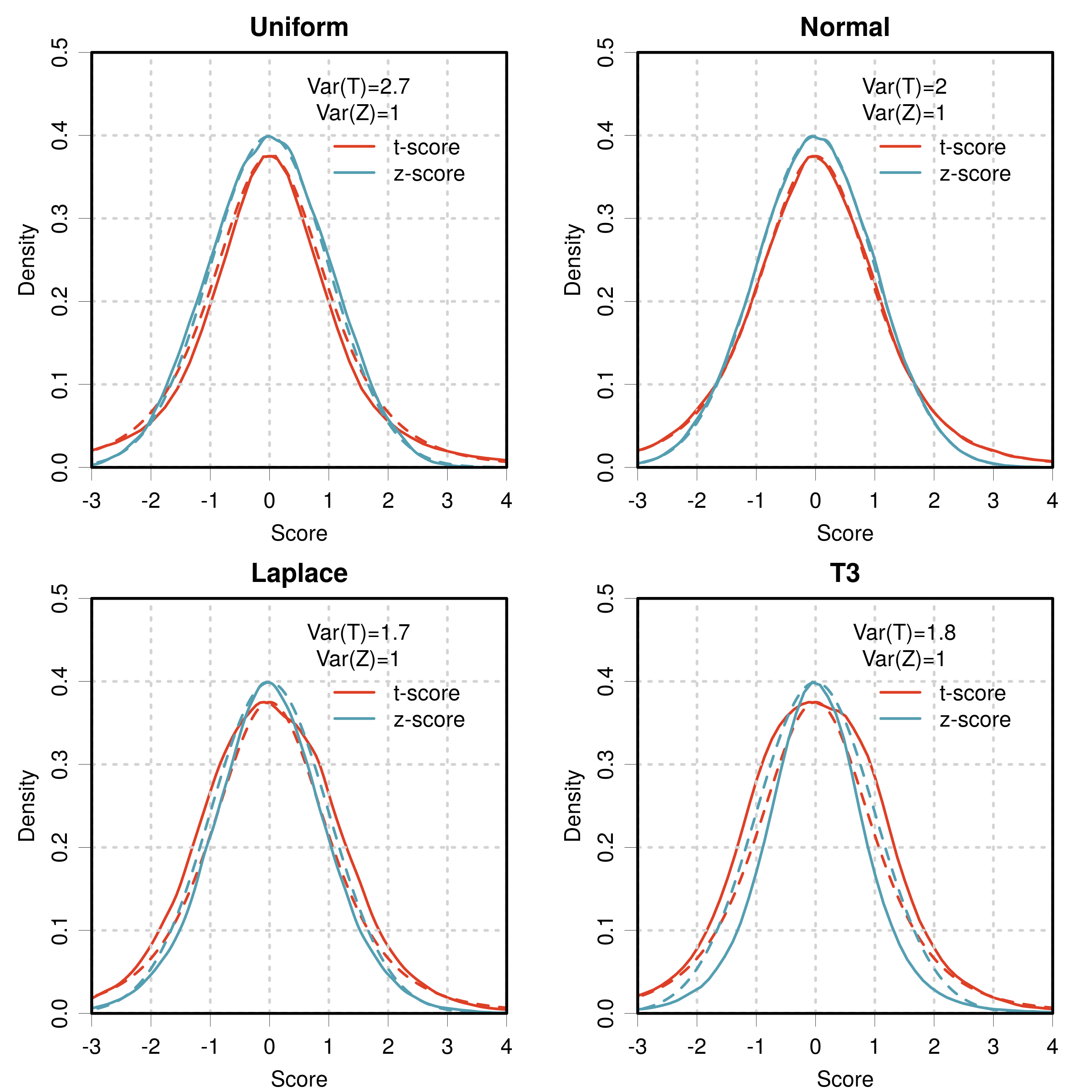
One can check that for the Normal error distribution, the t-scores and z-scores have the statistical properties described in Sect. V.3. For other generative distributions, the t- and z-score distributions deviate from the normal references. In spite of this, is independent of the generative distribution (and equal to 1 for those calibrated datasets), while depends strongly on the generative distribution. More specifically, there seems to be a reverse dependence between and the kurtosis of generative distribution, as shown in Table 2.
| Distribution | ||
|---|---|---|
| Beta(0.5,0.5) | 1.5 | 5.5 |
| Uniform(-1,1) | 1.8 | 2.7 |
| Exp4 | 2.18 | 2.4 |
| Normal | 3.0 | 2.0 |
| Exp1 | 6.0 | 1.7 |
| T3 | 1.7 |
The impact of the generative error distribution on decreases when the sample size increases (see Fig. 12). For practical purposes, one might consider the uniform and T3 distribution as extreme cases, as the Beta(0.5,0.5) distribution, displaying a concentration at the extremities of the variable range is not a very plausible predictive distribution, and there is not much variation left beyond . One might therefore consider to test t-scores calibration by . For smaller sample sizes (), one should allow for some margin around this value, within the limits shown in Fig. 12. These limits can be improved if information about the generative error distribution is available.
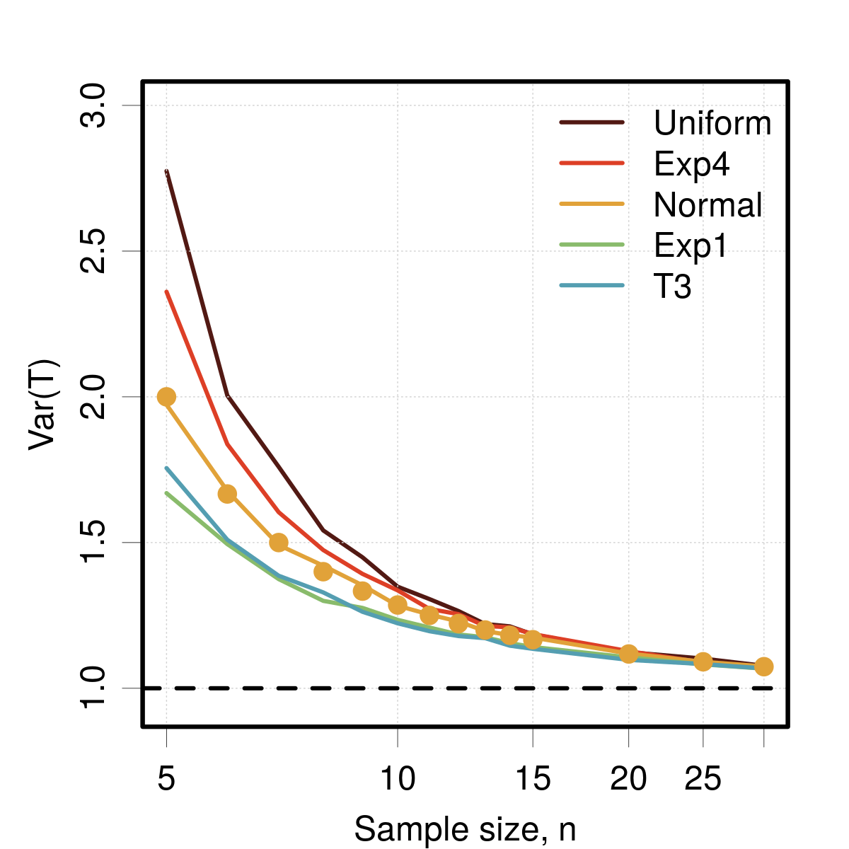
Appendix C Validation of tightness for small ensembles
Considering the inherent distribution of the standard uncertainties, testing if the uncertainties provide a good scale for the errors might be strongly perturbed, notably for heteroscedastic datasets where it is impossible to disambiguate structural uncertainty variability from the standard uncertainty statistical noise.
C.1 Homoscedastic case
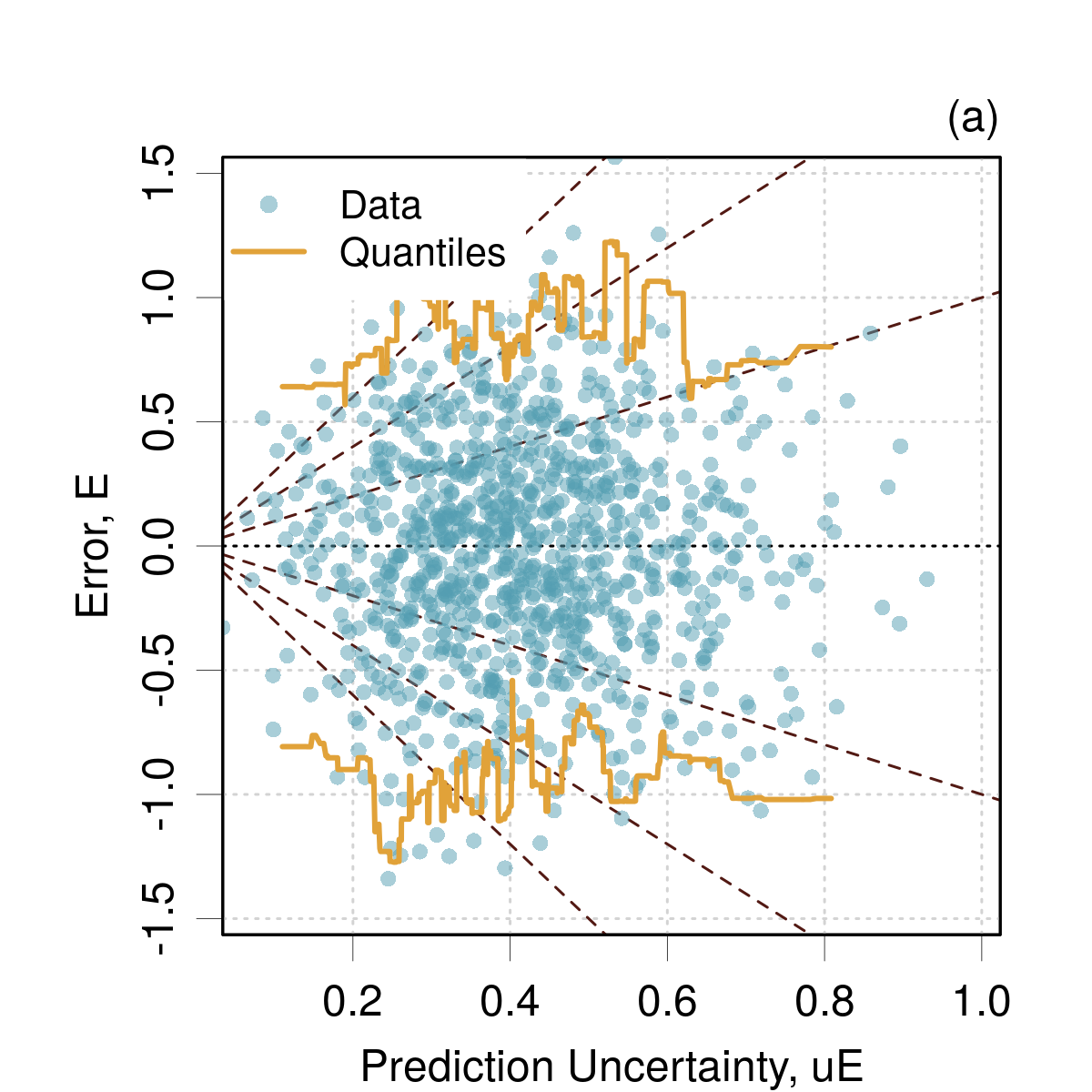
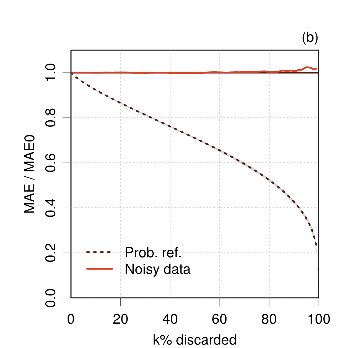
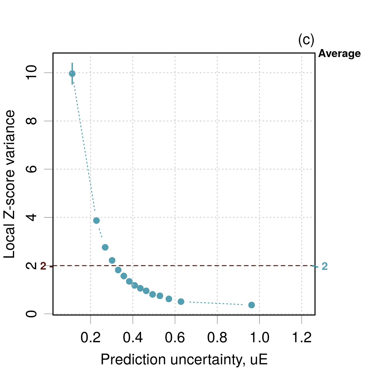
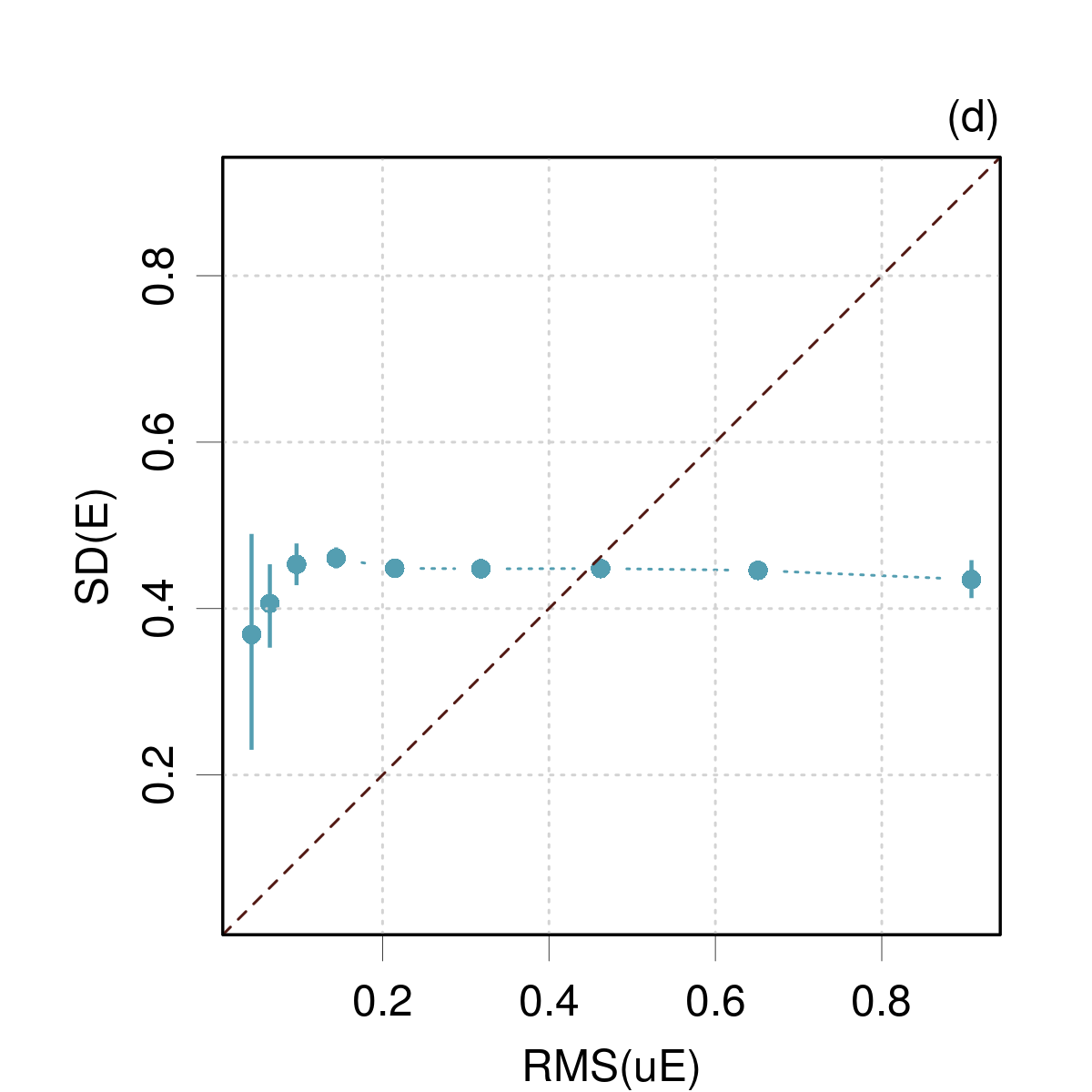
Considering the dataset for the normal generative distribution used in Fig. 11, which theoretically corresponds to an homoscedastic model, one can still make a plot because of the variability of the standard deviation [Fig. 13(a)]. From this plot, one would conclude on the absence of tightness, as there is no correlation between mean values and standard uncertainties, which is confirmed by the flat confidence curve [Fig. 13(b)]. The LZV analysis [Fig. 13(c)] shows that the average calibration is indeed correct ( for ), but the local analysis with respect to is not usable (a local analysis wrt. the calculated value might still be useful though). The LZV analysis is confirmed by the reliability diagram [Fig. 13(d)].
C.2 Heteroscedastic case

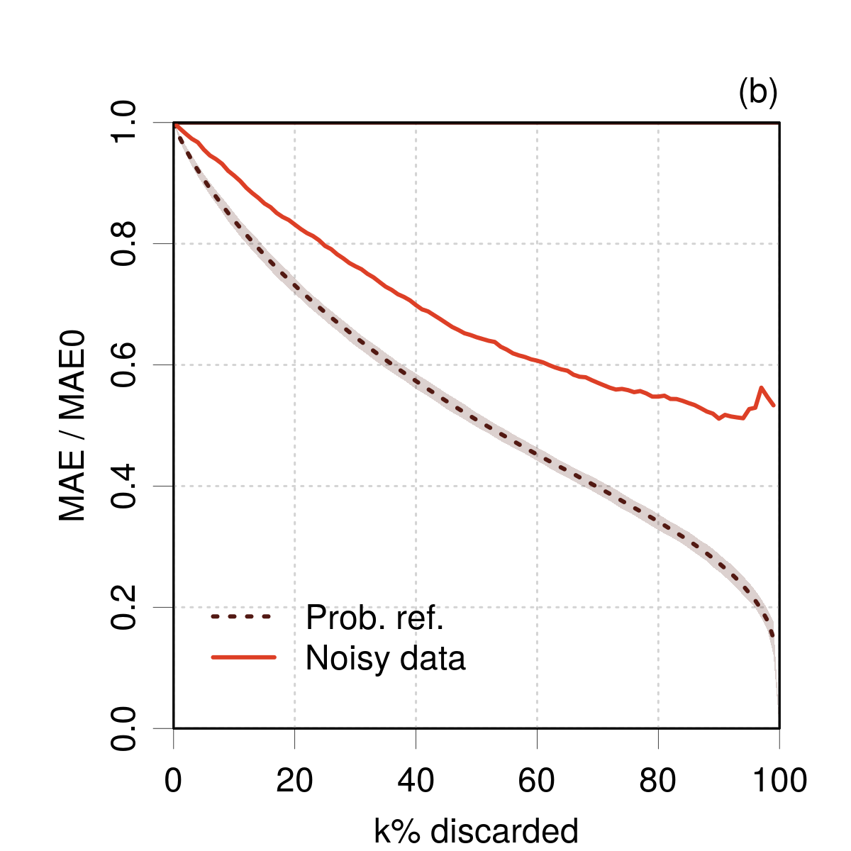
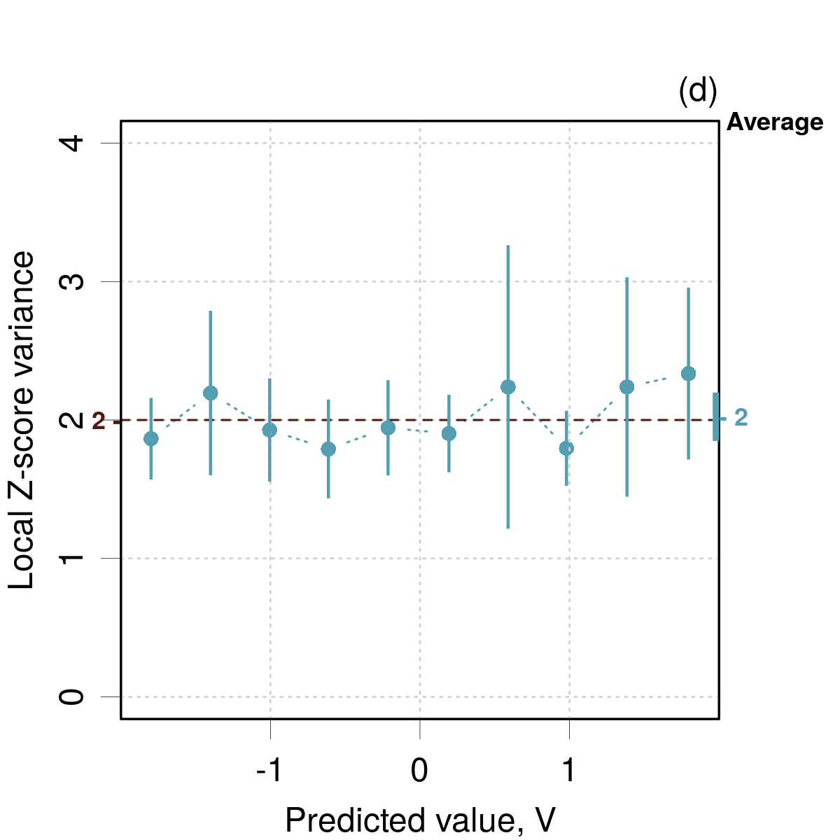
For the SYNT01 dataset, the perturbation introduced by using mean and standard error of ensembles () can be appreciated in Fig. 14. Comparison of the plot [Fig. 14(a)] to the one for the initial data [Fig. 1(b)] shows that the dataset is problematic. On the other hand, the confidence curve is continuously decreasing [Fig. 14(b)], although it does not match the probabilistic reference. As for the purely noisy example above, the LZV analysis wrt. reveals a correct average calibration but fails at the local tests [Fig. 14(c)]. However, a LZV analysis wrt. does not reveal any problem [Fig. 14(d)].
The situation for is slightly improved, however, the confidence curve and the LZV analysis wrt. would still lead to reject tightness [Fig. 15].