Graphene on a ferromagnetic substrate: instability of the electronic liquid

Abstract

We previously show [JETP Letters, 114, 763 (2021)] that a graphene sample placed on a ferromagnetic substrate demonstrates a cooperative magnetoelectronic instability. The instability induces a gap in the electronic spectrum and a canting deformation of the magnetization near the graphene-substrate interface. In this paper we prove that the interaction between the electrons in graphene strongly enhances the instability. Our estimates suggest that in the presence of even a moderate interaction the instability can be sufficiently pronounced to be detected experimentally in a realistic setting.

I Introduction

A graphene sheet placed on a ferromagnetic insulating substrate [1, 2, 3, 4] may be viewed as a prototypical graphene-spintronic [5] device. In such a heterostructure, due to the magnetic proximity effect, the spins of the graphene electrons are polarized. This polarization is accompanied by emergence of the Fermi surfaces in both graphene valleys, turning the graphene, which is a semi-metal in its pristine form, into a self-doped metal. Experimental study of such a graphene-based magnetic metal have been reported in Ref. 2, for example. As for theoretical studies dedicated to this, and similar, setups, one can mention Refs. [6, 7, 8].

In our recent paper [9] we have demonstrated that, at low temperature, a graphene sample placed in an insulating ferromagnetic substrate experiences a cooperative magnetoelectronic instability: due to the Fermi surface nesting, the perfect homogeneous ferromagnetic polarizations of both the graphene and the substrate experience canting, while the gap opens in the single-electron spectrum of the graphene. As a result of the instability, the magnetic metal becomes a magnetic semiconductor (that is, an insulator with a small gap).

To offer an intuitive and clear picture of the mechanism behind the instability, the presentation of Ref. 9 was made intentionally simple. An unfortunate downside of this approach is its diminishing reliability. The purpose of the present paper is to develop a more accurate description of the instability under study.

The simplifications incorporated into the theoretical model of Ref. 9 are of two sorts: (i) all single-electron states whose energies $\varepsilon_{\bf k}$ lie too far from the Fermi energy were neglected (specifically, all states with $|\varepsilon_{\bf k}|$ exceeding $\sim~{}1$ eV were omitted), (ii) the electron-electron interaction in graphene was ignored. Of these two, assumption (i) is purely technical: its only role was to justify the use of linear density of states (DOS) for graphene. It can be amended without introducing new concepts to the theoretical formalism of Ref. 9. The situation with (ii) is more complex, and requires more advanced theoretical apparatus.

The present paper addresses both (i) and (ii). Namely, we use the tight-binding DOS to account for all $p_{z}$ electronic states. Most importantly, we explicitly include a (Hubbard-like) interaction into the model. The interaction is then treated at the mean field level.

We will see that both modifications to the formalism act to increase the instability strength and the gap value relative to the expressions derived in Ref. 9. This makes it easier to argue that the instability may be observed in an experiment under realistic conditions.

Beside this, our formalism allows us to reveal the interaction-strength-driven crossover between magnetoelectronic instability (which relies on cooperation between the magnetic and electronic subsystems) to a more common spin-density wave (SDW) instability of purely electronic origin.

The paper is organized as follows. In Sec. II we describe the geometrical aspects of the studied heterostructure. The model Hamiltonian is introduced in Sec. III. The magnetoelectronic instability is discussed in Sec. IV, while the interaction effects are discussed in Sec. V. Section VI is reserved for the discussion of the paper’s main results and the conclusions. Technically involved derivations are relegated to Appendices.

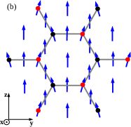
Figure 1: Schematic representation of a graphene sample on a ferromagnetic substrate. The orientation of the axes is shown in the lower left corner. The origin is at the center of the regular hexagon. Carbon atoms of graphene are represented by black (sublattice B) and red (sublattice A) circles. The solid (grey) lines connecting the atoms show carbon-carbon chemical bonds. There is a ferromagnetic substrate under graphene. Blue arrows represent local magnetization on the surface of the ferromagnet. Panel (a) corresponds to the case of perfect magnetization, see Eq. (11). Panel (b) represents the canted state. In this case, magnetization projection $M_{y}$ varies in space periodically, see Eqs. (16) and (17). We consider only those canting deformations, for which $M_{y}$ has opposite signs beneath the atoms belonging to different sublattices, in agreement with condition (17). One can easily recognize in panel (b) that $M_{y}>0$ beneath the atoms of $A$ sublattice, and $M_{y}<0$ for $B$ sublattice.

II Geometry considerations

The main object of our study is a graphene sample placed on a ferromagnetic substrate. Below we assume that the graphene lies in the $Oyz$ plane, while the $Ox$-axis is perpendicular to the substrate and directed away from it surfaces, see Fig. 1 (a). This is a “non-canonical” orientation of the coordinate system (usually it is assumed that graphene is located in the $Oxy$ plane). However, our choice makes description of the magnetic subsystem more conventional, since it will allow us to use $Oz$ as the spin quantization axis. Symbols $\hat{e}_{x,y,z}$ denote the unit vectors in the direction of the corresponding axes. To specify a point on the substrate surface we will use two-dimensional vectors ${\bf R}=y\hat{e}_{y}+z\hat{e}_{z}$ while a point inside the substrate is specified by vector ${\bf r}=x\hat{e}_{x}+y\hat{e}_{y}+z\hat{e}_{z}$, $x<0$, with $x=0$ being the substrate surface.

The graphene lattice is described by elementary translation vectors

$${\bf a}_{1,2}=\frac{\sqrt{3}}{2}a_{0}\left(\sqrt{3}\hat{e}_{y}\pm\hat{e}_{z}\right),$$ (1)

where $a_{0}$ is the distance between neighboring carbon atoms in graphene. Lattice sites coordinates on the sublattices $A$ and $B$ are given by the vectors

$${\bf R}_{A,B}={\bf a}_{1}n_{1}+{\bf a}_{2}n_{2}\mp a_{0}\hat{e}_{y},\quad n_{1,2}\in\mathbb{Z}.$$ (2)

In Fig. 1 lattice sites corresponding to different sublattices are depicted in different colors.

Finally, let us remind that the Brillouin zone in graphene has the shape of a regular hexagon, and the expression

$${\bf b}_{1,2}=\frac{2\pi}{3a_{0}}(\hat{e}_{y}\pm\sqrt{3}\hat{e}_{z})$$ (3)

specifies the reciprocal lattice vectors for graphene.

III Model for the graphene on a ferromagnetic substrate

Our model Hamiltonian describing electrons on the hexagonal lattice of graphene placed in contact with the ferromagnetic substrate reads

$$\hat{H}=\hat{H}_{0}+\hat{H}_{\rm Z}+\hat{H}_{\rm HB}.$$ (4)

Here $\hat{H}_{0}$ is the usual tight-binding Hamiltonian of the graphene

$$\hat{H}_{0}=-t\sum_{\langle\mathbf{R}_{A},\mathbf{R}_{B}\rangle,\,\sigma}\hat{d}_{\mathbf{R}_{A}\sigma}^{{\dagger}}\hat{d}_{\mathbf{R}_{B}\sigma}^{\vphantom{\dagger}}+{\rm H.c.}$$ (5)

In this expression the summation runs over the nearest-neighbor pairs ${\langle\mathbf{R}_{A},\mathbf{R}_{B}\rangle}$ and spin projection $\sigma$. Symbol $t$ denotes the hopping integral (for calculations one can use $t\approx 2.7$ eV).

Interaction between the electrons is described by the Hubbard term

$$\hat{H}_{\rm HB}=U\sum_{{\bf R}_{\alpha}}\hat{n}_{{\bf R}_{\alpha}\uparrow}\hat{n}_{{\bf R}_{\alpha}\downarrow},$$ (6)

$$\text{where}\quad\hat{n}_{{\bf R}_{\alpha}\sigma}=\hat{d}_{\mathbf{R}_{\alpha}\sigma}^{{\dagger}}\hat{d}_{\mathbf{R}_{\alpha}\sigma}^{\vphantom{\dagger}},$$ (7)

is the electron number operator and $\alpha=A,B$ is the sublattice index. Finally, the Zeeman term $\hat{H}_{\rm Z}$ induced due to the proximity to magnetic substrate equals to

$$\hat{H}_{\rm Z}=\sum_{{\bf R}_{\alpha}}{\bf h}_{{\bf R}_{\alpha}}\cdot\hat{\bf S}_{{\bf R}_{\alpha}}.$$ (8)

In this formula the electron spin operator $\hat{\bf S}_{{\bf R}_{\alpha}}$ is defined by a familiar expression

$$\hat{S}_{{\bf R}_{\alpha}}^{j}=\left(\begin{matrix}\hat{d}_{\mathbf{R}_{\alpha}\uparrow}^{{\dagger}}\hat{d}_{\mathbf{R}_{\alpha}\downarrow}^{{\dagger}}\end{matrix}\right)\hat{\sigma}^{j}\left(\begin{matrix}\hat{d}_{\mathbf{R}_{\alpha}\uparrow}^{\vphantom{\dagger}}\\ \hat{d}_{\mathbf{R}_{\alpha}\downarrow}^{\vphantom{\dagger}}\end{matrix}\right),$$ (9)

where $\hat{\sigma}^{j}$ are the Pauli matrices. Quantity ${\bf h}_{{\bf R}_{\alpha}}$ in $\hat{H}_{\rm Z}$ is the exchange field experienced by electrons on sublattice $\alpha$, on unit cell ${\bf R}$. We will assume that there is simple proportionality relation between ${\bf h}_{{\bf R}_{\alpha}}$ and local substrate magnetization ${\bf M}({\bf r})$

$${\bf h}_{{\bf R}_{\alpha}}=\tau{\bf M}(0,{\bf R}_{\alpha}).$$ (10)

In this relation, coefficient $\tau$ represents the strength of the magnetic proximity effect. Equation (10) implies that the Zeeman field at a specific carbon atom is proportional to the substrate magnetization directly beneath this atom.

For vanishing interaction $U=0$ and homogeneous ferromagnetic magnetization

$${\bf M}=M(0,0,1),\quad M>0,$$ (11)

the Hamiltonian $\hat{H}$ reads

$$\hat{H}=\sum_{\mathbf{q}}\hat{\Phi}_{\bf q}^{\dagger}\hat{\cal H}_{\bf q}^{\vphantom{{\dagger}}}\hat{\Phi}_{\bf q}^{\vphantom{{\dagger}}},$$ (12)

where $\hat{\Phi}_{\bf q}=\left(\hat{d}_{\mathbf{q}A\uparrow},\hat{d}_{\mathbf{q}B\uparrow},\hat{d}_{\mathbf{q}A\downarrow},\hat{d}_{\mathbf{q}B\downarrow}\right)^{T}$ is a bi-spinor operator corresponding to states with quasimomentum $\bf q$. In this expression $\hat{d}_{{\bf q}\alpha\sigma}$ is annihilation operator of electron with quasi-momentum ${\bf q}$, located on sublattice $\alpha$ with spin $\sigma=\uparrow,\downarrow$. Matrix $\hat{\cal H}_{\bf q}$ reads

$$\hat{\cal H}_{\bf q}=\left(\begin{matrix}h&-tf_{\mathbf{q}}&0&0\\ -tf_{\mathbf{q}}^{*}&h&0&0\\ 0&0&-h&-tf_{\mathbf{q}}\\ 0&0&-tf_{\mathbf{q}}^{*}&-h\end{matrix}\right),$$ (13)

where local Zeeman field $h$ equals to $h=\tau M$, and function $f_{\mathbf{q}}$ can be expressed as

$$f_{\bf q}=\left[1+2\exp{\left(\frac{3ia_{0}q_{y}}{2}\right)\cos{\left(\frac{\sqrt{3}a_{0}q_{z}}{2}\right)}}\right].$$ (14)

Diagonalizing $\hat{\cal H}_{\bf q}$ we derive electron dispersion for graphene on ferromagnetic substrate

$$\varepsilon^{(1,2,3,4)}_{\bf q}=\pm h\pm t|f_{\bf q}|.$$ (15)

This expression demonstrate that in the presence of the magnetic substrate the electronic structure is composed of four non-degenerate bands. Two of them cross Fermi level, forming circular Fermi surface around each non-equivalent Dirac points. Resultant dispersion is shown in Fig. 2.

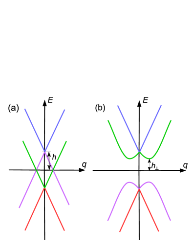
Figure 2: Schematic representation of the low-energy electron dispersion for graphene on a ferromagnetic substrate. The horizontal axis represents the two-dimensional momentum space. Energy is shown on the vertical axis. The origin corresponds to the Dirac point (the spectrum is identical near both Dirac points). For electronic states with spin $\sigma=\uparrow$ ($\sigma=\downarrow$), the apex of the Dirac cone is shifted by $h$ (shifted by $-h$). The dispersion for the perfectly homogeneous magnetization is plotted in (a). The band shown by the blue (red) line is completely empty (filled). The purple and green lines correspond to the bands crossing the Fermi level. These bands form an electron and a hole Fermi surface. The electron and hole Fermi surfaces coincide, exhibiting the perfect nesting with zero nesting vector. The insulating state with the canted magnetization is presented in (b). The filled bands (red and purple curves) contain mixed electronic states resulting from the hybridization of electron and hole states. The empty bands are shown in green and blue. The spectrum possesses a gap of $2h_{\perp}$.

Note that the Fermi surface is formed without external doping. In other words, the Zeeman field leads to self-doping effect: the electrons leave the $\sigma=\uparrow$ band, accumulating instead in the $\sigma=\downarrow$ band, generating two Fermi surface components. Due to this spin-dependent mechanism, the emerged Fermi surfaces are not spin-degenerate, unlike the situation in an ordinary metal.

Another important property of this electronic structure is the nesting of the Fermi surface. That is, the hole Fermi surface (formed by single-particle states with spin $\sigma=\uparrow$) coincides with the electronic Fermi surface (formed by single-particle states with spin $\sigma=\downarrow$). It is well known that a Fermi surface with nesting loses its stability when collective effects are taken into account. Indeed, the nesting is one of the major ingredients underpinning the mechanism of the magnetoelectronic instability discussed in our Ref. 9.

Finally, let us comment that inclusion of repulsive interaction $U>0$ into the model introduces several modifications to the non-interacting electronic state described in the previous paragraphs. For one, finite electron-electron interaction renormalizes Zeeman susceptibility. This effect is weak, as we will see below. More importantly, however, the interaction may induce a transition into an SDW phase (see, for example, Ref. 10 for a related discussion). Our investigation will show that, at low temperature, two incipient instabilities (SDW and magnetoelectronic) interact and mutually enhance each other.

IV Magnetoelectronic instability

For completeness, we briefly outline the origin of the magnetoelectronic instability for non-interacting electrons $U=0$ (more details can be found in our Ref. 9). Imagine that the perfect ferromagnetic order in the substrate [described by expression (11)] is distorted by weak canting deformation along $Oy$ axis

$$\mathbf{M}=M\left(0,\,m,\,1+O(m^{2})\right),$$ (16)

where $m=m(\mathbf{r})=m(x,{\bf R})$, $|m|\ll 1$, represents the deviation of magnetization from axis $Oz$.

The canting increases the magnetic energy of the substrate $E_{\rm m}$. One can expect that weak deformation $m$ leads to quadratic correction to the magnetic energy: $\delta E_{\rm m}=O(m^{2})$, and $\delta E_{\rm m}>0$. Due to non-zero $m$, the graphene electrons experience non-uniform Zeeman field. As long as $h=\tau Mm$ is small, it is possible to rely on the second-order perturbation theory to evaluate the graphene-electron energy correction $\delta E_{\rm e}$ caused by $m$. As it is always the case for second-order corrections, $\delta E_{\rm e}$ is non-positive ($\delta E_{\rm e}\leq 0$), but in the limit of small $\tau$ and $M$ the total energy increases ($\delta E_{\rm m}+\delta E_{\rm e}>0$), implying the overall stability of the homogeneous ferromagnetic configuration and the corresponding band structure.

Yet, there is a special type of canting $m$, for which this stability argument does not work. We explained in Ref. 9 that, because of the nested Fermi surface in our heterostructure, it is possible to construct $m=m({\bf r})$ such that the corresponding correction $\delta E_{\rm e}$ is no longer perturbative, but rather non-analytical, and the total correction $\delta E_{\rm m}+\delta E_{\rm e}$ may become negative for suitable choice of parameters. This is the origin of the magnetoelectronic instability.

To make our reasoning more concrete, let us consider $m$ such that $m=m_{\perp}>0$ under carbon atoms belonging to sublattice $A$, and $m=-m_{\perp}<0$ under atoms of sublattice $B$. In other words,

$$m(0,{\bf R}_{A})=-m(0,{\bf R}_{B})=m_{\perp}\,.$$ (17)

Schematically, the state with such a canting deformation is shown in Fig. 1 (b). Deeper in the substrate and away from its surface, the homogeneous magnetizations is restored [that is, $m(x,{\bf R})\rightarrow 0$ when $x\rightarrow-\infty$].

Formally speaking, the canting deformations satisfying Eq. (17) induce the hybridization between the electrons and holes at the Fermi energy. Such a hybridization leads to the gap opening and non-analytical contributions. Our calculations in this section will prove this fact explicitly. As for the more general, symmetry-based, discussion of this matter, interested readers may consult Refs. 10, 11.

For the canting (17), the order-of-magnitude estimate for correction is, then, $\delta E_{\rm m}\sim JM^{2}m_{\perp}^{2}{\cal N}_{\rm g}$, where ${\cal N}_{\rm g}$ is number of the unit cells in the graphene sample, and $J$ is the ferromagnetic exchange constant. For a specific model of the ferromagnetic substrate we derive (see Appendix A)

$$\delta{\cal E}_{\rm m}=\frac{\pi}{3\sqrt{3}}\frac{\zeta_{\perp}^{2}T_{\rm C}}{\zeta_{0}^{2}t},$$ (18)

where $\delta{\cal E}_{\rm m}=\delta E_{\rm m}/({\cal N}_{\rm g}t)$ is the normalized magnetic energy per unit cell, and $\zeta_{0}$ and $\zeta_{\perp}$ are two dimensionless Zeeman fields

$$\zeta_{0}=\frac{h}{t},\quad\zeta_{\perp}=\frac{h_{\perp}}{t}\,.$$ (19)

To calculate the energy of the electrons we need to find the band structure in the presence of the canting (17). Since in this Section we neglect the electron-electron interaction ($U=0$) the Hamiltonian for the graphene electrons may be expressed as in Eq. (12), with matrix ${\cal H}_{\bf q}$ being equal to

$$\hat{\cal H}_{\bf q}=\left(\begin{matrix}h&-tf_{\mathbf{q}}&-ih_{\perp}&0\\ -tf_{\mathbf{q}}^{*}&h&0&ih_{\perp}\\ ih_{\perp}&0&-h&-tf_{\mathbf{q}}\\ 0&-ih_{\perp}&-tf_{\mathbf{q}}^{*}&-h\end{matrix}\right),$$ (20)

where

$$h_{\perp}=\tau Mm_{\perp}.$$ (21)

Note that $h_{\perp}$ preserves the translation symmetry of the hexagonal lattice, but it does violate the symmetry between the two sublattices.

Diagonalizing ${\cal H}_{\bf q}$ one finds the dispersion in the presence of the canting deformation (17)

$$\varepsilon^{(1,2,3,4)}_{\mathbf{q}}=\pm\sqrt{h_{\perp}^{2}+\left(h\pm t|f_{\mathbf{q}}|\right)^{2}}\,.$$ (22)

The spectrum is plotted in Fig. 2 (b).

The total electronic energy of graphene can be expressed as $E_{\rm e}=t{\cal N}_{\rm g}{\cal E}_{\rm e}$, where the total dimensionless energy ${\cal E}_{\rm e}$ is a sum of two contributions coming from two bands ${\cal E}_{\rm e}={\cal E}_{+}+{\cal E}_{-}$ defined as

$${\cal E}_{\pm}=-\int_{0}^{3}d\zeta\,\rho(\zeta)\sqrt{\zeta_{\perp}^{2}+\left(\zeta_{0}\pm\zeta\right)^{2}}.$$ (23)

In this equation, the dimensionless honeycomb lattice DOS

$$\rho(\zeta)=\int\frac{d^{2}\mathbf{k}}{V_{\rm BZ}}\delta\left(\zeta-|f_{\mathbf{k}}|\right)$$ (24)

was introduced. For small $|\zeta|$ one can derive

$$\rho(\zeta)=\frac{2|\zeta|}{\sqrt{3}\pi}+\frac{2|\zeta|^{3/2}}{3\pi}+\ldots,$$ (25)

which is a generalization of the well-known expression for the linear asymptotic of the graphene DOS.

Straightforward mathematical analysis of the expression for ${\cal E}_{-}$ reveals that, at small $m_{\perp}$,

$${\cal E}_{-}(\zeta_{\perp})\approx{\cal E}_{-}(0)+2\rho(\zeta_{0})\zeta_{\perp}^{2}\ln\zeta_{\perp}+\ldots,$$ (26)

where the ellipsis stands for the terms which are less singular. We see that, due to the $m_{\perp}^{2}\ln m_{\perp}$ term, the total energy of the heterostructure always decreases when $m_{\perp}$ departs from zero, indicating the instability of the homogeneous ferromagnetic state.

The equilibrium value of $m_{\perp}$ is the solution of the minimization condition

$$\frac{\partial}{\partial\zeta_{\perp}}\left({\cal E}_{\rm e}+\delta{\cal E}_{m}\right)=0.$$ (27)

It is solved in Appendix B, where we derive the following expression for the dimensionless field $\zeta_{\perp}$

$$\zeta_{\perp}=\sqrt{12\zeta_{0}}\exp{\left[\frac{\sqrt{3}\pi}{4\zeta_{0}}\left(\eta(\zeta_{0})-\frac{2\pi T_{\rm C}}{3\sqrt{3}\zeta_{0}^{2}t}\right)\right]}.$$ (28)

Function $\eta(\zeta_{0})$ in this expression is defined as

$$\eta(\zeta_{0})=\int_{0}^{3}\frac{\left[\rho(\zeta)-\rho(\zeta_{0})\right]d\,\zeta}{\zeta-\zeta_{0}}+\int_{0}^{3}\frac{\rho(\zeta)d\,\zeta}{\zeta+\zeta_{0}}.$$ (29)

At small $\zeta_{0}$ one can demonstrate (see Appendix C) that

$$\eta(\zeta_{0})\approx 2I-\frac{2\zeta_{0}}{\sqrt{3}\pi}\ln\left(\frac{3}{\zeta_{0}}\right),$$ (30)

where the constant $I\approx 0.89$ is evaluated numerically. This approximation allows us to simplify Eq. (28)

$$\zeta_{\perp}=2\zeta_{0}\exp\left(\frac{C}{\zeta_{0}}-\frac{\pi^{2}T_{\rm C}}{6\zeta_{0}^{3}t}\right).$$ (31)

The coefficient $C$ in this formula is $C\approx 2.42$. The order parameter equals to

$$h_{\perp}=t\zeta_{\perp}=2h\exp{\left(\frac{Ct}{h}-\frac{\pi^{2}T_{\rm C}t^{2}}{6h^{3}}\right)},$$ (32)

while the spectral gap is $2h_{\perp}$. This relation for the gap can be compared against Eq. (45) of Ref. 9. It is easy to see that, while the general structure of these two expressions are almost identical, the gap value we found above always exceeds the value found in Ref. 9. This is a consequence of the more advanced treatment of the higher-energy single-electron states.

V Effects of the electron-electron interaction

In this section we discuss how electron-electron interaction influences the magnetoelectronic instability. Specifically we will re-derive Eq. (32) in a model with $U>0$. To reach this goal, we will use the mean field (MF) approximation. There are several (perfectly equivalent) formulations to the MF approach. Below we will use the variational version of the MF. To this end we introduce the MF Hamiltonian

$$\hat{H}^{\rm MF}=\sum_{\mathbf{q}}\hat{\Phi}_{\bf q}^{\dagger}\hat{\cal H}_{\bf q}^{\rm MF}\hat{\Phi}_{\bf q}^{\vphantom{{\dagger}}},$$ (33)

$$\hat{\cal H}_{\bf q}^{\rm MF}=t\left(\begin{matrix}\tilde{\zeta}_{0}&-f_{\mathbf{q}}&-i\tilde{\zeta}_{\perp}&0\\ -f_{\mathbf{q}}^{*}&\tilde{\zeta}_{0}&0&i\tilde{\zeta}_{\perp}\\ i\tilde{\zeta}_{\perp}&0&-\tilde{\zeta}_{0}&-f_{\mathbf{q}}\\ 0&-i\tilde{\zeta}_{\perp}&-f_{\mathbf{q}}^{*}&-\tilde{\zeta}_{0}\end{matrix}\right).$$ (34)

The ground state $\left|\Psi_{\rm MF}\right>$ of $\hat{H}^{\rm MF}$ acts as our variational wave function. Dimensionless quantities $\tilde{\zeta}_{0}$ and $\tilde{\zeta}_{\perp}$ will serve as the optimization parameters for our variational ansatz. Matrix $\hat{\cal H}_{\bf q}^{\rm MF}$ has the same structure as $\hat{\cal H}_{\bf q}$ in Eq. (20). In other words, we assume that the interaction renormalizes parameters $\zeta_{0}$ and $\zeta_{\perp}$ responsible for the magnetoelectronic instability. As we will see below, this renormalization accounts for the interaction-driven enhancement of the instability.

Using the symbol $\langle\ldots\rangle$ to denote matrix element with respect to $\left|\Psi_{\rm MF}\right>$, we can express the total dimensionless variational energy as

$${\cal E}^{\rm var}=({\cal N}_{\rm g}t)^{-1}\langle\hat{H}\rangle+\delta{\cal E}_{\rm m}.$$ (35)

Adjusting $\zeta_{\perp}$, $\tilde{\zeta}_{0}$, and $\tilde{\zeta}_{\perp}$, the minimum of ${\cal E}^{\rm var}$ must be found. Differentiating ${\cal E}^{\rm var}$ with respect to $\tilde{\zeta}_{\perp}$, we obtain

$$2t\left(\zeta_{\perp}-\tilde{\zeta}_{\perp}\right)-U\langle S^{y}\rangle=0,$$ (36)

where $\langle S^{y}\rangle$ is the average magnetization projection on a site belonging to the sublattice $A$, that is $\langle S^{y}_{{\bf R}_{A}}\rangle=\langle S^{y}\rangle$. Using the Hellmann -Feynman theorem (see Appendix D), we derive

$$\langle S^{y}\rangle=-\frac{\tilde{\zeta}_{\perp}}{2}\left[\eta(\zeta_{0})+\frac{2\tilde{\zeta}_{0}}{\sqrt{3}\pi}\ln{\left(\frac{12\tilde{\zeta}_{0}}{\tilde{\zeta}_{\perp}^{2}}\right)}\right].$$ (37)

Note that $\langle S^{y}_{{\bf R}_{B}}\rangle=-\langle S^{y}\rangle$. In other words, the average magnetization $y$-projections have different signs on different sublattices. (For $z$ axis one has $\langle S^{z}_{{\bf R}_{A}}\rangle=\langle S^{z}_{{\bf R}_{B}}\rangle=\langle S^{z}\rangle$.)

Differentiation over $\tilde{\zeta}_{0}$ allows us to obtain the second mean field equation

$$2t\left(\zeta_{0}-\tilde{\zeta}_{0}\right)-U\langle S^{z}\rangle=0.$$ (38)

As above, to calculate $\langle S^{z}\rangle$, one can invoke the Hellmann -Feynman theorem and find

$$\langle S^{z}\rangle\approx-\frac{\sqrt{3}}{\pi}\tilde{\zeta}_{0}^{2}.$$ (39)

Deriving this relation, we used Eq. (25) valid for small $\tilde{\zeta}_{0}$. Since $\langle S^{z}\rangle=O(\tilde{\zeta}_{0}^{2})$, the last term in Eq. (38) can be neglected, and we conclude

$$\tilde{\zeta}_{0}\approx\zeta_{0}.$$ (40)

This formula implies that the interaction does not introduce significant renormalization to the homogeneous Zeeman field induced by the substrate.

Finally, we minimize ${\cal E}^{\rm var}$ with respect to $\zeta_{\perp}$. We obtain

$$\frac{\partial{\cal E}^{\rm var}}{\partial\zeta_{\perp}}=2\langle S^{y}\rangle+\frac{2\pi}{3\sqrt{3}}\frac{T_{\rm C}}{t\zeta_{0}^{2}}\zeta_{\perp}=0.$$ (41)

Collecting Eqs. (41), (38) and (37), we obtain the following system of equation

$$\begin{cases}\zeta_{\perp}-\tilde{\zeta}_{\perp}=\frac{U}{2t}\langle S^{y}\rangle,\\ -2\langle S^{y}\rangle=\frac{2\pi}{3\sqrt{3}}\frac{T_{\rm C}}{t\zeta_{0}^{2}}\zeta_{\perp}\\ -2\langle S^{y}\rangle=\tilde{\zeta}_{\perp}\left(\eta(\zeta_{0})+\frac{2\zeta_{0}}{\sqrt{3}\pi}\ln{\left|\frac{12\zeta_{0}}{\tilde{\zeta}_{\perp}^{2}}\right|}\right),\end{cases}$$ (42)

where the last equation can be simplified with the help of Eq. (30) Solving this system, one determines $\tilde{\zeta}_{\perp}$ and finds the order parameter $h_{\perp}=t\tilde{\zeta}_{\perp}$

$$h_{\perp}=2h\exp\left(\frac{Ct}{h}-\frac{\sqrt{3}\pi^{2}T_{\rm C}t^{2}}{6\sqrt{3}h^{3}+\pi UT_{\rm C}h}\right).\quad$$ (43)

This expression coincide with Eq. (28) in the limit of vanishing $U$, as expected. The gap increases when $U$ grows. The resultant values of $h_{\perp}$ versus $U$ are plotted in Fig. 3 for various parameters choices.

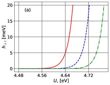
Figure 3: Order parameter $h_{\perp}$ as function of the interaction parameter $U$, for various $T_{\rm C}$, on linear (a) and log (b) scale. Solid (red) curve for $T_{\rm C}=16$ K, dashed (blue) curve for $T_{\rm C}=17$ K, dashed-dotted (green) curve for $T_{\rm C}=18$ K. For these curves we use $h=20$ meV (or, equivalently, $h=300$ T).

VI Discussion

In the previous sections we demonstrated that graphene on a ferromagnetic substrate is susceptible to cooperative magnetoelectronic instability. Near the interface between the substrate and the graphene the instability generates finite canting deformation of the ferromagnetic polarization. The canting, in turn, leads to the spectral gap in the electronic spectrum of the graphene. Our analysis generalizes the study of Ref. 9 to include the effects of finite electron-electron interaction. As Eq. (43) proves, the interaction enhances the instability.

The instability can be potentially detected in a transport experiment measuring the temperature dependence of the graphene conductivity $\sigma=\sigma(T)$. The instability will manifest itself as a sharp decrease of $\sigma(T)$ when $T$ drops below the characteristic energy scale $\sim h_{\perp}$. This implies that, for the instability to be observable in experiment, the value of $h_{\perp}$ must be sufficiently large. To assess $h_{\perp}$, one can examine Fig. 3, which shows the plots of $h_{\perp}$ versus $U$ for different values of $T_{\rm C}$. The graphs in the latter figure reveals that, while at $U=0$ the order parameter might be very weak, a realistic electron-electron interaction drastically, by orders of magnitude, enhances the equilibrium value of $h_{\perp}$, making it sufficiently strong to be detected in an experiment. Specifically, for the superstructure of graphene on EuS substrate, described in Ref. 2, one has $T_{\rm C}=16$ K and $h=300$ T (equivalently, $h=20$ meV). For such parameters $h_{\perp}\gtrsim 10$ meV for $U\gtrsim 4.65$ eV. Examining Eq. (43) for $h_{\perp}$ we notice that, as far as the interaction strength $U$ is concerned, two regimes can be identified. To illustrate this, let us re-write Eq. (43) as follows

$$h_{\perp}=2h\exp\left(\frac{Ct}{h}-\frac{\sqrt{3}\pi t^{2}/h}{U_{*}+U}\right),$$ (44)

where the characteristic interaction strength is

$$U_{*}=\frac{6\sqrt{3}h^{2}}{\pi T_{\rm C}}.$$ (45)

We see that, when $U\ll U_{*}$, one can neglect $U$ relative to $U_{*}$ in Eq. (44). In this limit, the effects of the interaction are weak, and the instability is driven exclusively by the cooperation between the substrate magnetic subsystem and the electrons of the graphene. This regime is studied in Ref. 9.

In the opposite case ($U\gg U_{*}$) one can treat $U_{*}$ as a small correction to $U$, neglecting $U_{*}$ in the zeroth-order approximation. If $U_{*}$ is removed from Eq. (44), then $T_{\rm C}$ does not enter the expression for $h_{\perp}$, indicating that the cooperation between the canting deformation and the electrons is no longer important. Instead, the only remaining role of the ferromagnetic substrate is to generate a Fermi surface with finite DOS $\rho\propto h$ at the Fermi energy. In this regime, the nested Fermi surface is driven into the SDW-like insulating state by the electron-electron interaction, as discussed in Ref. 10.

The two regimes are connected by a crossover which occurs at $U\sim U_{*}$. In the crossover region, both electron-electron interaction effects and the canting deformation in the substrate cooperate together equally to induce the instability.

To conclude, we studied the influence of the electron-electron interaction on the magnetoelectronic instability in graphene on the ferromagnetic substrate. We demonstrated that the interaction enhances the instability significantly: even a moderate strength interaction can increase the characteristic energy scale by several orders of magnitude. Our findings suggest that the instability could be detected experimentally in realistic settings.

Appendix A Magnetic energy correction

In this appendix we calculate the magnetic energy of the substrate with and without the canting deformation of the ferromagnetic magnetization. Our starting point is the Weiss model of a ferromagnet. In the Weiss approximation, the magnetic energy of the substrate is

$$E_{m}=-\frac{J}{2}\sum_{i\bm{\delta}}\mathbf{M}_{{\bf r}_{i}}\mathbf{M}_{{\bf r}_{i}+\bm{\delta}}\,.$$ (46)

Here $J$ is the exchange integral, ${\bf r}_{i}$ denotes position of $i$’th “atom” in three-dimensional lattice of the substrate, vectors $\bm{\delta}$ link a given atom with its nearest neighbors, and ${\bf M}_{{\bf r}_{i}}$ is the magnetization on the $i$’th atom. We assume that vectors ${\bf M}_{{\bf r}_{i}}$ have the same length: $|{\bf M}_{{\bf r}_{i}}|=M$ for any $i$.

For a model of this type, we can derive expression for Curie temperature:

$$T_{\rm C}=\frac{JM^{2}Z}{3},$$ (47)

where $Z$ is the number of the nearest neighbors of an atom. This expression can be obtained using the mean-field method applied to energy (46). The advantage of Eq. (47) stems from the fact that it allows us to estimate $J$, using often-available experimental data for the Curie temperature, low-temperature substrate magnetization $M$, and $Z$.

Denoting the number of atoms in the substrate as ${\cal N}$, we can express the energy of the perfectly ordered ferromagnetic configuration as

$$E_{\|}=-\frac{\cal N}{2}ZJM^{2}\,,$$ (48)

which is valid at $T\ll T_{\rm C}$. For configurations with weak and smooth deviations from the homogeneously ordered state the energy becomes $E_{m}\approx E_{\|}+\delta E_{\rm m}$, where the correction $\delta E_{\rm m}$ equals to

$$\delta E_{m}\approx\frac{JM^{2}}{2a_{0}}\int_{V}\!\!(\nabla m)^{2}dV\,,$$ (49)

where we assumed that substrate material has cubic lattice ($Z=6$) whose lattice constant is $a_{0}$ (generalizations beyond these two assumptions are trivial). The dimensionless cant $m=m({\bf r})$, $|m|\ll 1$, is introduced by Eq. (16). It is treated here as a function of a three-dimensional continuous variable ${\bf r}=(x,{\bf R})$, while integration in Eq. (49) is performed over the volume of the substrate ($x<0$).

We now want to apply Eq. (49) for the evaluation of the magnetic energy increase $\delta E_{\rm m}$ caused by the canting deformation shown in Fig. 1 (b). Our goal is (i) to find $m$ which satisfies boundary condition (17) at $x=0$, while (ii) delivering the minimum to the functional (49).

However, the boundary condition (17) was formulated for a function on a lattice. For a continuous approximation that we employ in this Appendix, such a boundary condition is incomplete. Indeed, it fixes the values of $m$ on a discrete set of points only, thus, on $\mathbb{R}^{2}$, there are infinitely many non-identical functions satisfying Eq. (17). To mend this problem we extend the boundary condition

$$m(0,{\bf R})=-\frac{2}{3\sqrt{3}}m_{\perp}\sum_{\mathbf{K}}\sin{(\mathbf{K}\mathbf{R})}\,,\quad{\bf R}\in\mathbb{R}^{2}.$$ (50)

where vector $\mathbf{K}$ runs over the following list of values

$$\mathbf{K}=\mathbf{b}_{1},\quad\mathbf{K}=\mathbf{b}_{2},\quad\mathbf{K}=-\mathbf{b}_{1}-\mathbf{b}_{2}.$$ (51)

The advantage of this sum is that not only it is compatible with the Eq. (17), but it contains the minimum number (six) of plane waves, while all spatial frequencies $|{\bf K}|=4\pi/(3a_{0})$ have the lowest possible values compatible with Eq. (17). Adding more plane waves with shorter wave lengths leads to more positive contributions to the functional $\delta E_{\rm m}$.

To proceed with (i) and (ii) formulated above, we derive the Laplace equation

$$\nabla^{2}m=0\,,$$ (52)

for $m$ within the substrate, with Eq. (50) at the interface. The solution to this mathematical problem is

$$m(\mathbf{r})=-\frac{2}{3\sqrt{3}}m_{\perp}\exp{\left(|\mathbf{K}|x\right)}\sum_{\mathbf{K}}\sin{(\mathbf{K}\mathbf{R})}\,.$$ (53)

This expression demonstrates that, as expected, the canting deformation of the magnetization is the strongest directly at the surface ($x=0$), but it quickly decreases deep into the substrate. Substituting this $m=m({\bf r})$ into Eq. (49), we obtain

$$\delta E_{m}=\frac{4\pi}{27}\frac{Jm_{\perp}^{2}M^{2}{\cal S}}{a_{0}^{2}}=\frac{4\pi}{27}\frac{Jh_{\perp}^{2}{\cal S}}{a_{0}^{2}\tau^{2}}\,.$$ (54)

Alternatively, we can write using dimensionless quantities that

$$\delta{\cal E}_{m}=\frac{\pi}{3\sqrt{3}}\frac{\zeta_{\perp}^{2}T_{\rm C}}{\zeta_{0}^{2}t}.$$ (55)

As we mentioned in Sec. IV, the magnetic energy associated with the cant is quadratic in $m_{\perp}$ and does not contain any non-analytic contributions.

Appendix B Single-particle gap value

In this Appendix we provide detailed derivation of Eq. (28) for the dimensionless order parameter $\zeta_{\perp}$. The calculations presented below improves the derivation of Eq. (30) in Ref. 12. Our starting point is Eq. (27) which we expand as follows

$$\frac{\partial\left({\cal E}_{1}+{\cal E}_{2}+\delta{\cal E}_{m}\right)}{\partial\zeta_{\perp}}=\zeta_{\perp}\left(-\int_{0}^{3}\frac{\rho(\zeta)d\,\zeta}{\sqrt{\zeta_{\perp}^{2}+\left(\zeta-\zeta_{0}\right)^{2}}}-\int_{0}^{3}\frac{\rho(\zeta)d\,\zeta}{\sqrt{\zeta_{\perp}^{2}+\left(\zeta+\zeta_{0}\right)^{2}}}+\frac{2\pi}{3\sqrt{3}}\frac{T_{\rm C}}{\zeta_{0}^{2}t}\right)\approx$$ (56)

$$\approx\zeta_{\perp}\left(\frac{2\pi}{3\sqrt{3}}\frac{T_{\rm C}}{\zeta_{0}^{2}t}-\rho(\zeta_{0})\int_{0}^{3}\frac{d\,\zeta}{\sqrt{\zeta_{\perp}^{2}+\left(\zeta-\zeta_{0}\right)^{2}}}-\eta(\zeta_{0})\right)=0,$$

where function $\eta(\zeta_{0})$ is defined by Eq. (29). The integral $\rho(\zeta_{0})\int_{0}^{3}{d\,\zeta}(\zeta_{\perp}^{2}+\left(\zeta-\zeta_{0}\right)^{2})^{-1/2}$ in (56) can be found explicitly

$$\rho(\zeta_{0})\int_{0}^{3}\frac{d\,\zeta}{\sqrt{\zeta_{\perp}^{2}+\left(\zeta-\zeta_{0}\right)^{2}}}\approx\frac{2\zeta_{0}}{\sqrt{3}\pi}\ln{\left(\frac{12\zeta_{0}}{\zeta_{\perp}^{2}}\right)}.$$ (57)

As a result we can solve equation (56) and obtain value of $\zeta_{\perp}$

$$\zeta_{\perp}=\sqrt{12\zeta_{0}}\exp{\left\{\frac{\sqrt{3}\pi}{4\zeta_{0}}\left(\eta(\zeta_{0})-\frac{2\pi T_{\rm C}}{3\sqrt{3}\zeta_{0}^{2}t}\right)\right\}},$$ (58)

which is Eq. (28).

Appendix C Approximation for $\eta(\zeta_{0})$

In this Appendix we derive the approximate form for $\eta(\zeta_{0})$ valid in the limit of small $\zeta_{0}$. We start by noting that the low-$\zeta_{0}$ singularities of the integral $\int_{0}^{3}d\,\zeta{\left[\rho(\zeta)-\rho(\zeta_{0})\right]}/{|\zeta-\zeta_{0}|}$ are weak, and it is sufficient to to approximate the integral by a constant

$$\int_{0}^{3}\frac{\left[\rho(\zeta)-\rho(\zeta_{0})\right]d\,\zeta}{|\zeta-\zeta_{0}|}=I+O(\zeta_{0}),$$ (59)

$$I=\int_{0}^{3}\frac{\rho(\zeta)d\zeta}{\zeta}\approx 0.89.$$ (60)

To prove that the ignored terms in Eq. (59) are indeed $O(\zeta_{0})$, we split the integration interval into two sub-intervals $\int_{0}^{3}\ldots=\int_{0}^{\zeta^{*}}\ldots+\int_{\zeta^{*}}^{3}\ldots$, where $\zeta^{*}$ satisfies $\zeta_{0}<\zeta^{*}\ll 1$. One can write

$$\int_{\zeta^{*}}^{3}\frac{\left[\rho(\zeta)-\rho(\zeta_{0})\right]d\,\zeta}{|\zeta-\zeta_{0}|}=\int_{\zeta^{*}}^{3}\frac{\rho(\zeta)d\,\zeta}{\zeta}-$$ (61)

$$\rho(\zeta_{0})\int_{\zeta^{*}}^{3}\frac{d\,\zeta}{\zeta-\zeta_{0}}+\zeta_{0}\int_{\zeta^{*}}^{3}\frac{\rho(\zeta)d\,\zeta}{\zeta(\zeta-\zeta_{0})}.$$

In the right-hand side of this relation, the integrands are non-singular for $\zeta^{*}<\zeta<3$. The first integral is independent of $\zeta_{0}$, while two other explicitly belong to $O(\zeta_{0})$ class.

As for the integral from 0 to $\zeta^{*}$, due to smallness of $\zeta^{*}$, the expansion (25) can be used. Thus

$$\frac{\rho(\zeta)-\rho(\zeta_{0})}{\zeta-\zeta_{0}}\approx\frac{2}{\sqrt{3}\pi}+\frac{2\sqrt{\zeta}}{3\pi}+\frac{2\zeta_{0}}{3\pi(\sqrt{\zeta_{0}}+\sqrt{\zeta})}.$$ (62)

Deriving this representation we used the following relation $\frac{x^{3/2}-y^{3/2}}{x-y}=\frac{x+\sqrt{xy}+y}{x^{1/2}+y^{1/2}}.$We see from Eq. (62) that the integral over the sub-interval $(0,\zeta^{*})$ equals to a $\zeta_{0}$-independent constant plus $O(\zeta_{0})$ corrections, as Eq. (59) implies.

The second integral in Eq. (29) can be transformed as follows

$$\int_{0}^{3}\frac{\rho(\zeta)d\,\zeta}{\zeta+\zeta_{0}}=\int_{0}^{3}\frac{\rho d\zeta}{\zeta}+\int_{0}^{3}d\zeta\left[\frac{\rho}{\zeta_{0}+\zeta}-\frac{\rho}{\zeta}\right]$$ (63)

$$=I-\zeta_{0}\int_{0}^{3}\frac{\rho d\zeta}{\zeta(\zeta+\zeta_{0})}.$$

To estimate $\int_{0}^{3}{d\zeta\rho(\zeta)}/[\zeta(\zeta+\zeta_{0})]$, we re-write it to show explicitly the most singular contribution

$$\int\!\!\frac{\rho d\zeta}{\zeta(\zeta\!+\!\zeta_{0})}\!=\!\frac{2}{\sqrt{3}\pi}\ln\!\left(\!\frac{3}{\zeta_{0}}\!\right)\!+\!\int\!\frac{\left[(\rho/\zeta)\!-\!\rho^{\prime}(0)\right]\!d\zeta}{\zeta+\zeta_{0}}.$$ (64)

The remaining integral is finite in the limit $\zeta_{0}\rightarrow 0$, as can be proven with the help of Eq. (25). To evaluate it numerically we divide the integration interval into two parts

$$\int_{0}^{3}\frac{\left[(\rho/\zeta)-\rho^{\prime}(0)\right]d\zeta}{\zeta+\zeta_{0}}=\int^{\zeta^{*}}_{0}\frac{\left[(\rho/\zeta)-\rho^{\prime}(0)\right]d\zeta}{\zeta+\zeta_{0}}$$ (65)

$$+\int^{3}_{\zeta^{*}}\frac{\left[(\rho/\zeta)-\rho^{\prime}(0)\right]d\zeta}{\zeta+\zeta_{0}}.$$

The usefulness of this representation stems from the fact that numerically evaluated numerator has large error bars near zero $\zeta$. Fortunately, for small $\zeta^{*}$ and $0<\zeta<\zeta^{*}$ analytical approximation based on Eq. (25) can be used: $\rho(\zeta)/\zeta-\rho^{\prime}(0)={2\zeta^{1/2}}/(3\pi)$. Integral over the interval between $\zeta^{*}=0.2$ and 3, evaluated numerically, is found to be very small. Thus

$$\int_{0}^{3}\frac{\left[(\rho/\zeta)-\rho^{\prime}(0)\right]d\zeta}{\zeta+\zeta_{0}}\approx\frac{4}{3\pi}\sqrt{\zeta^{*}}\approx 0.2$$ (66)

for $\zeta^{*}=0.2$. Collecting all terms, we find

$$\eta(\zeta_{0})=2I-\frac{2\zeta_{0}}{\sqrt{3}\pi}\ln\left(\frac{3}{\zeta_{0}}\right)+O(\zeta_{0}),$$ (67)

where the retained terms are more singular than those which were ignored. This expression is the basis for Eq. (30).

Appendix D Mean field equations derivations

In this Appendix we will provide additional technical details for the mean field equations derivations. Our goal is to differentiate ${\cal E}^{\rm var}$, defined by Eq. (35), over the variational parameters $\zeta_{\perp}$, $\tilde{\zeta}_{0}$, and $\tilde{\zeta}_{\perp}$. With this in mind, it is convenient to express ${\cal E}^{\rm var}$ in the following manner

$${\cal E}^{\rm var}=({\cal N}_{\rm g}t)^{-1}\left(\langle\hat{H}^{\rm MF}\rangle+\langle\delta\hat{H}\rangle+\langle\hat{H}_{\rm HB}\rangle\right)+\delta{\cal E}_{\rm m}.\qquad$$ (68)

In brief, this representation explicitly splits $\langle\hat{H}\rangle$ into three terms: (i) the mean field energy $\langle\hat{H}^{\rm MF}\rangle$, (ii) the interaction term $\langle\hat{H}_{\rm HB}\rangle$, and (iii) all other contributions $\langle\delta\hat{H}\rangle$. The Hamiltonian in (iii) is bilinear in single-electron operators

$$\delta\hat{H}=\sum_{\mathbf{q}}\hat{\Phi}_{\bf q}^{\dagger}\delta\hat{\cal H}\hat{\Phi}_{\bf q}^{\vphantom{{\dagger}}},$$ (69)

its associated matrix $\delta\hat{\cal H}$ equals to

$$\delta\hat{\cal H}=t\left(\begin{matrix}\delta\zeta_{0}&0&-i\delta\zeta_{\perp}&0\\ 0&\delta\zeta_{0}&0&i\delta\zeta_{\perp}\\ i\delta\zeta_{\perp}&0&-\delta\zeta_{0}&0\\ 0&-i\delta\zeta_{\perp}&0&-\delta\zeta_{0}\end{matrix}\right),$$ (70)

where $\delta\zeta_{0}=\zeta_{0}-\tilde{\zeta}_{0}$, and $\delta\zeta_{\perp}=\zeta_{\perp}-\tilde{\zeta}_{\perp}$.

Let us differentiate ${\cal E}^{\rm var}$ over $\tilde{\zeta}_{\perp}$. The term $\delta{\cal E}_{\rm m}$ is independent of $\tilde{\zeta}_{\perp}$, thus the corresponding derivative vanishes. The Hellmann-Feynman theorem allows us to establish that

$$\frac{\partial\langle\hat{H}^{\rm MF}\rangle}{\partial\tilde{\zeta}_{\perp}}=2t\langle S^{y}\rangle{\cal N}_{\rm g}.$$ (71)

Here we used the relation $\langle S^{y}_{{\bf R}_{A}}\rangle=-\langle S^{y}_{{\bf R}_{B}}\rangle=\langle S^{y}\rangle$ which connects magnetization projections on the two sublattices.

To calculate the derivatives for two other terms in Eq. (68) we can write explicit expressions for them

$$\langle\delta\hat{H}\rangle=2t\left(\delta\zeta_{0}\langle S_{z}\rangle+\delta\zeta_{\perp}\langle S_{y}\rangle\right){\cal N}_{\rm g},$$ (72)

$$\langle\hat{H}_{\rm HB}\rangle=\frac{U}{2}\left(1-\langle S_{z}\rangle^{2}-\langle S_{y}\rangle^{2}\right){\cal N}_{\rm g}.$$ (73)

Therefore

$$\frac{\partial\langle\delta\hat{H}\rangle}{\partial\tilde{\zeta}_{\perp}}=2t\left(-\langle S_{y}\rangle+\delta\zeta_{\perp}\frac{\partial\langle S_{y}\rangle}{\partial\tilde{\zeta}_{\perp}}\right){\cal N}_{\rm g},$$ (74)

$$\frac{\partial\langle\hat{H}_{\rm HB}\rangle}{\partial\tilde{\zeta}_{\perp}}=-U\langle S_{y}\rangle\frac{\partial\langle S_{y}\rangle}{\partial\tilde{\zeta}_{\perp}}{\cal N}_{\rm g}.$$ (75)

Collecting all contributions, we obtain

$$\frac{\partial{\cal E}^{\rm var}}{\partial\tilde{\zeta}_{\perp}}=\left(2\delta\zeta_{\perp}-\frac{U}{t}\langle S_{y}\rangle\right)\frac{\partial\langle S_{y}\rangle}{\partial\tilde{\zeta}_{\perp}}.$$ (76)

Equating the latter with zero one recovers Eq. (36). Two other mean field equations are derived using similar tactics.

Finally, we want to outline the derivation of expression (37) for $\langle S^{y}\rangle$. The most convenient approach is to use Eq. (71). The mean field energy is

$$\langle\hat{H}^{\rm MF}\rangle=-{\cal N}_{\rm g}t\int_{0}^{3}d\zeta\,\rho\sqrt{\tilde{\zeta}_{\perp}^{2}+\left(\tilde{\zeta}_{0}-\zeta\right)^{2}}-$$ (77)

$${\cal N}_{\rm g}t\int_{0}^{3}d\zeta\,\rho\sqrt{\tilde{\zeta}_{\perp}^{2}+\left(\tilde{\zeta}_{0}+\zeta\right)^{2}}.\quad$$

Substituting this expression into Eq. (71), one derives

$$2\langle S^{y}\rangle=-\tilde{\zeta}_{\perp}\int_{0}^{3}\frac{\rho(\zeta)d\zeta}{\sqrt{\tilde{\zeta}_{\perp}^{2}+\left(\tilde{\zeta}_{0}-\zeta\right)^{2}}}-$$ (78)

$$\tilde{\zeta}_{\perp}\int_{0}^{3}\frac{\rho(\zeta)d\zeta}{\sqrt{\tilde{\zeta}_{\perp}^{2}+\left(\tilde{\zeta}_{0}+\zeta\right)^{2}}}.$$

The derivation steps discussed in Appendix B allows one to recover Eq. (37) from Eq. (78).

References

Wang et al. [2015]
Z. Wang,
C. Tang,
R. Sachs,
Y. Barlas, and
J. Shi,
“Proximity-Induced Ferromagnetism in Graphene Revealed by
the Anomalous Hall Effect,” Phys. Rev. Lett.
114, 016603
(2015).
Wei et al. [2016]
P. Wei,
S. Lee,
F. Lemaitre,
L. Pinel,
D. Cutaia,
W. Cha,
F. Katmis,
Y. Zhu,
D. Heiman,
J. Hone, et al.,
“Strong interfacial exchange field in the graphene/EuS
heterostructure,” Nat. Mater.
15, 711 (2016).
Mendes et al. [2015]
J. B. S. Mendes,
O. Alves Santos,
L. M. Meireles,
R. G. Lacerda,
L. H. Vilela-Leão,
F. L. A. Machado,
R. L. Rodríguez-Suárez,
A. Azevedo, and
S. M. Rezende,
“Spin-Current to Charge-Current Conversion and
Magnetoresistance in a Hybrid Structure of Graphene and Yttrium Iron
Garnet,” Phys. Rev. Lett.
115, 226601
(2015).
Leutenantsmeyer
et al. [2016]
J. C. Leutenantsmeyer,
A. A. Kaverzin,
M. Wojtaszek,
and B. J. van
Wees, “Proximity induced room temperature ferromagnetism
in graphene probed with spin currents,” 2D Mater.
4, 014001 (2016).
Han et al. [2014]
W. Han,
R. K. Kawakami,
M. Gmitra, and
J. Fabian,
“Graphene spintronics,” Nat.
Nanotechnol. 9, 794
(2014).
Zollner et al. [2016]
K. Zollner,
M. Gmitra,
T. Frank, and
J. Fabian,
“Theory of proximity-induced exchange coupling in graphene
on hBN/(Co, Ni),” Phys. Rev. B
94, 155441
(2016).
Cardoso et al. [2018]
C. Cardoso,
D. Soriano,
N. A.
García-Martínez, and
J. Fernández-Rossier,
“Van der Waals Spin Valves,” Phys.
Rev. Lett. 121, 067701
(2018).
Zollner et al. [2018]
K. Zollner,
M. Gmitra, and
J. Fabian,
“Electrically tunable exchange splitting in bilayer
graphene on monolayer Cr2X2Te6 with X = Ge, Si, and Sn,”
New J. Phys. 20,
073007 (2018).
Dresvyankin et al. [2021]
D. N. Dresvyankin,
A. V. Rozhkov,
and A. O.
Sboychakov, “Magnetoelectronic Instability
of Graphene on a Ferromagnetic Substrate,” Pis’ma v
ZhETF 114, 824
(2021), [JETP Letters, 114, 763
(2021)].
Aleiner et al. [2007]
I. L. Aleiner,
D. E. Kharzeev,
and A. M.
Tsvelik, “Spontaneous symmetry breaking in
graphene subjected to an in-plane magnetic field,”
Phys. Rev. B 76,
195415 (2007).
Rakhmanov et al. [2012]
A. L. Rakhmanov,
A. V. Rozhkov,
A. O. Sboychakov,
and F. Nori,
“Instabilities of the -Stacked Graphene Bilayer,”
Phys. Rev. Lett. 109,
206801 (2012).
Sboychakov et al. [2013]
A. O. Sboychakov,
A. V. Rozhkov,
A. L. Rakhmanov,
and F. Nori,
“Antiferromagnetic states and phase separation in doped
AA-stacked graphene bilayers,” Phys. Rev. B
88, 045409
(2013).