Relativistic calculated K-shell level widths and fluorescence yields
for atoms with 20$\leq$Z$\leq$30

Abstract

The $K$-shell level radiative, non-radiative, and total widths, $K$-shell fluorescence yields and $K$-shell hole state lifetimes for atoms with 20$\leq$Z$\leq$30 have been calculated in fully-relativistic way using the extensive multiconfiguration Dirac-Fock calculations with the inclusion of the Breit interaction and QED corrections and also using multiconfiguration Dirac-Hartree-Slater calculations.

I Introduction

$K$-shell atomic level width, $\Gamma_{K}$, and fluorescence yields, $\omega_{K}$, have been an object of the intense research for several decades, both experimentally and theoretically, and a large number of articles have been published on these subjects. In 1969-70, McGuire McGuire (1969, 1970) was the first who published $\omega_{K}$ values for atoms with 4$\leq$Z$\leq$54. Then, in 1971, Walters and Balla Walters and Bhalla (1971) and Kostroun et al. Kostroun et al. (1971) published $\omega_{K}$ values for atoms with 5$\leq$Z$\leq$54 and 10$\leq$Z$\leq$70, respectively. These calculations were based on the Hartree-Fock-Slater method. In 1972, Bambynek et al. Bambynek et al. (1972) published a review article with a selection of the "most reliable" experimental and theoretical $\omega_{K}$ values for selected atoms with 13$\leq$Z$\leq$92. In 1979, Krause and Oliver published compilation of $\Gamma_{K}$ Krause and Oliver (1979) and $\omega_{K}$ Krause (1979) values for atoms with 5$\leq$Z$\leq$110, basing on both experimental and theoretical data. In 1980, Chen et al. Chen et al. (1980) published $\Gamma_{K}$ and $\omega_{K}$ values for selected atoms with 18$\leq$Z$\leq$96, calculated by using relativistic Dirac-Hartree-Slater method. Afterwards, in 1994, Hubbell et al. Hubbell et al. (1994) published a compilation of experimental and semi-empirical $\omega_{K}$ values for atoms with 3$\leq$Z$\leq$110. In 2001, Campbell and Papp presented Campbell and Papp (2001) a compilation of recommended $\Gamma_{K}$ values for atoms with 10$\leq$Z$\leq$92 basing on experimental data and earlier compilation of EADL Perkins et al. (1991) from 1991. Although these data are already several decades old and in the last years the more advanced relativistic methods have been developed, they are still widely used for comparison with experimental results.

The knowledge of natural $K$-shell level widths are a base for investigation of width of various $K$-shell X-ray lines; the comparison between theoretical and experimental X-ray linewidths leads to analysis of ionization mechanisms in the inner shells of atom (see eg. Polasik et al. (2011)). A good knowledge of $K$-shell fluorescence yields is important for the analysis of various measurements in the fields of nuclear, atomic, molecular, and applied physics (see eg. Bambynek et al. (1972)). On the other hand, in the last years, there have been many experimental high precision measurements of the $K$-shell fluorescence yields for atoms with 20$\leq$Z$\leq$30 Yashoda et al. (2005); Şahin et al. (2005); Gudennavar et al. (2003); Durak and Özdemır (2001); Şimşek et al. (2000); Söğüt (2010); Han et al. (2007), but the full agreement between experimental and theoretical or semi-empirical data was not obtained.

In this work the theoretical predictions for radiative, non-radiative, and total natural $K$-shell level widths, as well as $K$-shell fluorescence yields and $K$-shell hole state lifetimes, for atoms with 20$\leq$Z$\leq$30 have been evaluated basing on the multiconfiguration Dirac-Fock (MCDF) method and the multiconfiguration Dirac-Hartree-Slater (DHS) method. It is important to note that in case of open-shell atoms (when de-excitation concerns many states) every state has a specific width, thus, radiative and total widths presented in this work are the average values evaluated as an arithmetic mean of all widths for individual states.

II Theoretical background

II.1 Relativistic calculations

The methodology of MCDF calculations performed in the present studies is similar to the published earlier, in many papers (see, e.g., Grant et al. (1980a, b); Grant and J.McKenzie (1980); Hata and Grant (1983); Grant (1984); Dyall et al. (1989); Grant (1974, 1988); Polasik (1989, 1995)). The effective Hamiltonian for an N-electron system is expressed by

$$H=\sum_{i=1}^{N}h_{D}(i)+\sum_{j>i=1}^{N}C_{ij},$$ (1)

where $h_{D}(i)$ is the Dirac operator for $i$-th electron and the term $C_{ij}$ accounts for electron-electron interactions. The latter is a sum of the Coulomb interaction operator and the transverse Breit operator. An atomic state function (ASF) with the total angular momentum $J$ and parity $p$ is assumed in the form

$$\Psi_{s}(J^{p})=\sum_{m}c_{m}(s)\Phi(\gamma_{m}J^{p}),$$ (2)

where $\Phi(\gamma_{m}J^{p})$ is a configuration state function (CSF), $c_{m}(s)$ is a configuration mixing coefficient for state $s$, $\gamma_{m}$ represents all information required to define a certain CSF uniquely. Apart from the transverse Breit interaction two types of quantum electrodynamics (QED) corrections have been included (self-energy and vacuum polarization).

In general, the multiconfiguration DHS method is similar to the MCDF method, but simplified expression for electronic exchange integrals is used Gu (2008).

Table 1: Numbers of $K^{-1}$, $L_{2,3}^{-1}$, $M_{2,3}^{-1}$, $L^{-2}$, $L^{-1}M^{-1}$, $L^{-1}N^{-1}$, $M^{-2}$, $M^{-1}N^{-1}$ for considered valence electronic configurations.

Z	Atom	Valence	Number of states for spectator hole(s)
		configuration	$K^{-1}$	$L_{2,3}^{-1}$	$M_{2,3}^{-1}$	$L^{-2}$	$L^{-1}M^{-1}$	$L^{-1}N^{-1}$	$M^{-2}$	$M^{-1}N^{-1}$
20	Ca	$4s^{2}$	1	2	2	10	20	6	10	6
21	Sc	$3d^{1}4s^{2}$	4	12	12	53	122	31	56	32
22	Ti	$3d^{2}4s^{2}$	16	45	45	210	484	122	227	126
23	V	$3d^{3}4s^{2}$	38	110	110	493	1174	287	556	303
24	Cr	$3d^{5}4s^{1}$	144	417	417	1934	4858	288	2458	322
25	Mn	$3d^{5}4s^{2}$	74	214	214	967	2429	561	1229	624
26	Fe	$3d^{6}4s^{2}$	63	180	180	838	2172	486	1160	560
27	Co	$3d^{7}4s^{2}$	38	110	110	493	1356	287	773	350
28	Ni	$3d^{8}4s^{2}$	16	45	45	210	616	122	392	160
29	Cu	$3d^{10}4s^{1}$	2	4	4	16	66	3	63	5
30	Zn	$3d^{10}4s^{2}$	1	2	2	10	36	6	35	10

Table 2: Radiative level widths of $K^{-1}$ hole state atomic level for atoms with 20$\leq$Z$\leq$30 (Coulomb gauge).

Z	Atom	$\bar{X}_{i}$ [s-1]		$\sum_{i}\bar{X}_{i}$	$\Gamma^{Rad}$
		$K\alpha_{1,2}$ [$\times 10^{14}$]	$K\beta_{1,3}$ [$\times 10^{13}$]	[$\times 10^{14}$ s-1]	[eV]
20	Ca	1.737	2.412	1.978	0.130
21	Sc	2.167	2.827	2.449	0.161
22	Ti	2.670	3.531	3.023	0.199
23	V	3.257	4.351	3.692	0.243
24	Cr	3.935	5.142	4.450	0.293
25	Mn	4.712	6.391	5.351	0.352
26	Fe	5.599	7.635	6.362	0.419
27	Co	6.605	9.047	7.509	0.494
28	Ni	7.739	10.643	8.804	0.579
29	Cu	9.015	11.007	10.116	0.666
30	Zn	10.424	12.950	11.719	0.771

Table 3: Radiative level widths of $K^{-1}$ hole state atomic level for atoms with 20$\leq$Z$\leq$30 (Babushkin gauge).

Z	Atom	$\bar{X}_{i}$ [s-1]		$\sum_{i}\bar{X}_{i}$	$\Gamma^{Rad}$
		$K\alpha_{1,2}$ [$\times 10^{14}$]	$K\beta_{1,3}$ [$\times 10^{13}$]	[$\times 10^{14}$ s-1]	[eV]
20	Ca	1.579	2.758	1.855	0.122
21	Sc	1.985	3.202	2.305	0.152
22	Ti	2.459	3.974	2.856	0.188
23	V	3.012	4.868	3.499	0.230
24	Cr	3.654	5.726	4.227	0.278
25	Mn	4.391	7.074	5.098	0.336
26	Fe	5.234	8.411	6.075	0.400
27	Co	6.192	9.921	7.184	0.473
28	Ni	7.274	11.622	8.437	0.555
29	Cu	8.491	12.021	9.694	0.638
30	Zn	9.814	12.859	11.100	0.731

II.2 Lifetime of excited states, width of corresponding atomic levels, and fluorescence yields

Each excited state can be attributed by the mean lifetime $\tau$. The mean lifetime can be defined as time after which the number of excited states of atoms decreases $e$ times. The mean lifetime is determined by a total transition rate of de-excitation (radiative and non-radiative) processes $W_{i}$:

$$\tau=\left(\sum_{i}W_{i}\right)^{-1}=\left(\sum_{i}X_{i}+\sum_{j}A_{j}+\sum_{k}C_{k}\right)^{-1}\;,$$ (3)

where $X_{i}$ is a transition rate of radiative process, $A_{j}$ is a transition rate of non-radiative Auger process, and $C_{k}$ is a transition rate of non-radiative Coster-Kronig or super-Coster-Kronig process. De-excitation processes happen in all possible ways leading to lower energetic states allowed by selection rules.

Due to the energy-time uncertainty principle ($\Delta E\Delta t=\hbar$), the lifetime of excited state $\tau$ is connected with width of corresponding atomic level $\Gamma$ (note that for one atomic level there may be more than one corresponding excited states) by the relationship

$$\Gamma=\frac{\hbar}{\tau}=\hbar W=\hbar\sum_{i}W_{i}\;.$$ (4)

Natural width of atomic level can be obtained in form of a sum of radiative width $\Gamma_{X}$, Auger width $\Gamma_{A}$, and Coster-Kronig $\Gamma_{C}$ width; or, in other way, as a sum of radiative and non-radiative widths:

$$\Gamma=\Gamma_{X}+\Gamma_{A}+\Gamma_{C}=\Gamma^{Rad}+\Gamma^{Nrad}\;,$$ (5)

where $\Gamma^{Rad}=\Gamma_{X}$ and $\Gamma^{Nrad}=\Gamma_{A}+\Gamma_{C}$. The relevant yields are linked to the terms presented above, i.e.

$$\omega=\frac{\Gamma_{X}}{\Gamma}=\frac{\sum_{i}X_{i}}{\sum_{i}X_{i}+\sum_{j}A_{j}+\sum_{k}C_{k}}\;,$$ (6a)

$$a=\frac{\Gamma_{A}}{\Gamma}=\frac{\sum_{j}A_{j}}{\sum_{i}X_{i}+\sum_{j}A_{j}+\sum_{k}C_{k}}\;,$$ (6b)

$$f=\frac{\Gamma_{C}}{\Gamma}=\frac{\sum_{k}C_{k}}{\sum_{i}X_{i}+\sum_{j}A_{j}+\sum_{k}C_{k}}\;,$$ (6c)

where $\omega$ is fluorescence yield, $a$ is Auger yield, and $f$ is Coster-Kronig yield.

For open-shell atomic systems for each atomic hole level $(nlj)^{-\alpha}$ (where $\alpha$= 1, 2, …, $2j+1$) a great number of hole states $(nlj)_{J}{}^{-\alpha}$ are linked. Therefore, for $i$-th hole state all transition rates $W_{ij}$ corresponded to $j$-th de-excitation process should be considered. Radiative part of natural width $\Gamma^{Rad}_{i}$ of $i$-th hole state can be determined by using transition rate of radiative processes $X_{ij}$ according to the formula

$$\Gamma^{Rad}_{i}=\hbar\sum_{j}X_{ij}\;.$$ (7)

Radiative part of the natural width of $(nlj)^{-\alpha}$ hole atomic level is taken as the arithmetic mean of the radiative parts to the natural width of the each hole state $(nlj)_{J}{}^{-\alpha}$, i.e. according to the following formula

$$\Gamma^{Rad}=\frac{\sum_{i}\Gamma^{Rad}_{i}}{n}\;,$$ (8)

where $\Gamma^{Rad}$ is a radiative part of natural level width, and $n$ is a number of hole state corresponding to a given hole level.

Similarly, the non-radiative part of the natural width can be determined by calculating the transition rates for non-radiative Auger $A_{ij}$ and Coster-Kronig $C_{ik}$ processes according to the formula

$$\Gamma^{Nrad}=\frac{\hbar\left(\sum_{i,j}A_{ij}+\sum_{i,k}C_{ik}\right)}{n}\;,$$ (9)

where all the designations are analogous to those above. Then the total natural width of the atomic hole levels can be determined according to the Eq. 5.

Equations 7, 8, and 9 can be rewritten to the form of:

$$\Gamma^{Nrad}=\hbar\sum_{j}\bar{X}_{j}\;,$$ (10)

$$\Gamma^{Nrad}=\hbar\left(\sum_{j}\bar{A}_{j}+\sum_{k}\bar{C}_{k}\right)\;,$$ (11)

where $\bar{X}_{j}=\frac{1}{n}\sum_{i}X_{ij}$ is a mean value of transition rates per one $(nlj)_{J}{}^{-\alpha}$ hole state for $j$-th de-excitation channel, and for $\bar{A}$ and $\bar{C}$ similarly.

III Results and discussion

Considered radiative de-excitation processes for $K^{-1}$ hole states are: $K\alpha_{1,2}$ ($K$-$L_{2,3}$) and $K\beta_{1,3}$ ($K$-$M_{2,3}$). These are electric (E1) dipole transitions. Transitions of higher order (E2, M1, M2, etc.) were not included here due to the small contribution to the level widths. Considered radiative de-excitation processes are: $K$-$LL$, $K$-$LM$, $K$-$LN$, $K$-$MM$, and $K$-$MN$. It is worth noticing that in the case of $K^{-1}$ hole states there is no Coster-Kronig de-excitation process. For open-shell atoms, numerous states are engaged for these de-excitation channels (see Table 1).

The calculations of radiative transition rates were carried out by means of Grasp2k code Jönsson et al. (2007). The radiative transition rates were calculated in both Coulomb Grant (1974) and Babushkin Babushkin (1964) gauges. The calculations of non-radiative transition rates were carried out by means of both Fac code Gu (2003, 2008) and a piece of code from Ratip suite Fritzsche (2001, 2012), which uses Grasp92 Parpia et al. (1996) calculated wavefunctions. All the versions of Grasp code are fully MCDF codes. The Fac code is based on modified DHS method, but multiconfigurational approach and Breit interaction are also included.

Table 4: Non-radiative level widths of $K^{-1}$ hole state atomic level for atoms with 20$\leq$Z$\leq$30 (Fac calculated).

Z	Atom	$\bar{A}_{i}$ [s-1]					$\sum_{i}\bar{A}_{i}$	$\Gamma^{Nrad}$
		K-LL	K-LM	K-LN	K-MM	K-MN	[$\times 10^{15}$ s-1]	[eV]
		[$\times 10^{14}$]	[$\times 10^{14}$]	[$\times 10^{12}$]	[$\times 10^{13}$]	[$\times 10^{11}$]
20	Ca	7.744	1.677	4.388	0.918	5.318	0.956	0.629
21	Sc	8.022	1.774	4.364	0.990	5.388	0.994	0.655
22	Ti	8.282	1.862	4.319	1.054	5.411	1.030	0.678
23	V	8.525	1.944	4.264	1.113	5.404	1.063	0.700
24	Cr	8.761	1.983	1.844	1.123	2.316	1.088	0.716
25	Mn	8.965	2.095	4.137	1.222	5.340	1.123	0.739
26	Fe	9.165	2.166	4.072	1.274	5.296	1.150	0.757
27	Co	9.354	2.234	4.007	1.323	5.247	1.177	0.774
28	Ni	9.532	2.300	3.943	1.372	5.197	1.201	0.791
29	Cu	9.705	2.340	2.164	1.389	2.972	1.221	0.804
30	Zn	9.861	2.428	3.821	1.468	5.096	1.248	0.821

Table 5: Non-radiative level widths of $K^{-1}$ hole state atomic level for atoms with 20$\leq$Z$\leq$30 (Ratip calculated).

Z	Atom	Valence	$\bar{A}_{i}$ [s-1]			$\sum_{i}\bar{A}_{i}$	$\Gamma^{Nrad}$
		configurations	K-LL	K-LM	K-MM	[$\times 10^{15}$ s-1]	[eV]
			[$\times 10^{14}$]	[$\times 10^{14}$]	[$\times 10^{13}$]
20	Ca	$4s^{2}$	8.155	1.944	1.167	1.022	0.672
21	Sc	$3d_{3/2}^{1}4s^{2}$	8.356	2.064	1.278	1.055	0.694
22	Ti	$3d_{3/2}^{4}$	8.657	2.045	1.209	1.082	0.712
23	V	$3d_{3/2}^{4}4s^{1}$	8.834	2.196	1.362	1.117	0.735
24	Cr	$3d_{5/2}^{6}$	9.037	2.251	1.395	1.143	0.752
25	Mn	$3d_{5/2}^{6}4s^{1}$	9.204	2.375	1.521	1.173	0.772
26	Fe	$3d_{5/2}^{6}4s^{2}$	9.373	2.511	1.660	1.205	0.793
27	Co	$3d_{3/2}^{1}3d_{5/2}^{6}4s^{2}$	9.503	2.512	1.734	1.219	0.802
28	Ni	$3d^{10}$	9.693	2.533	1.642	1.239	0.816
29	Cu	$3d^{10}4s^{1}$	9.830	2.628	1.738	1.263	0.831
30	Zn	$3d^{10}4s^{2}$	9.969	2.813	1.930	1.297	0.854

Table 6: Total level widths of $K^{-1}$ hole state atomic level, and fluorescence yields and lifetimes of $K^{-1}$ hole states for atoms with 20$\leq$Z$\leq$30 for four calculation models (see text for details).

Z	Atom	$\Gamma$ [eV]				$\omega$				$\tau$ [$\times 10^{-16}$ s]
		C+F	B+F	C+R	B+R	C+F	B+F	C+R	B+R	C+F	B+F	C+R	B+R
20	Ca	0.760	0.751	0.803	0.795	0.171	0.162	0.162	0.154	8.666	8.759	8.201	8.284
21	Sc	0.816	0.806	0.855	0.846	0.198	0.188	0.188	0.179	8.069	8.164	7.694	7.780
22	Ti	0.877	0.866	0.911	0.900	0.227	0.217	0.218	0.209	7.507	7.602	7.222	7.311
23	V	0.943	0.930	0.978	0.965	0.258	0.248	0.248	0.239	6.983	7.079	6.730	6.819
24	Cr	1.009	0.994	1.045	1.030	0.290	0.280	0.280	0.270	6.524	6.620	6.299	6.388
25	Mn	1.091	1.075	1.124	1.108	0.323	0.312	0.313	0.303	6.031	6.125	5.854	5.942
26	Fe	1.176	1.157	1.212	1.193	0.356	0.346	0.346	0.335	5.597	5.688	5.431	5.517
27	Co	1.269	1.247	1.297	1.275	0.390	0.379	0.381	0.371	5.188	5.277	5.077	5.162
28	Ni	1.370	1.346	1.395	1.371	0.423	0.413	0.415	0.405	4.804	4.890	4.718	4.802
29	Cu	1.469	1.442	1.497	1.469	0.453	0.443	0.445	0.434	4.479	4.566	4.396	4.479
30	Zn	1.593	1.552	1.625	1.585	0.484	0.471	0.475	0.461	4.133	4.241	4.050	4.154

In Tables 2 and 3 the present calculated values of radiative part of natural $K^{-1}$ level width for atoms with 20$\leq$Z$\leq$30 are collected (in both Coulomb and Babushkin gauges). In Tables 4 and 5 the present calculated values of non-radiative part of natural $K^{-1}$ level width are collected (calculated with the use of both Fac and Ratip codes). In order to simplify the calculations and because of the restriction in number of simultaneously optimized states within Grasp92 code, in the case of non-radiative transition rates calculated by Ratip code the valence electronic configurations were simplified in order to minimize number of states. In fact, this approach can change values of non-radiative transition rates a little, but the tests show that it do not change the total value of non-radiative part of natural $K^{-1}$ level width substantially. The $K$-$LN$ and $K$-$MN$ non-radiative de-excitation channels are also omitted in this case, because of their minor contribution to the level width. For each of Tables 2, 3, 4, and 5, the values of present calculated radiative and non-radiative transition rates for considered de-excitation processes for $K^{-1}$ hole states are also shown in the form of mean values per one $K^{-1}$ hole state.

The total $K^{-1}$ level widths, the fluorescence yields and the lifetimes of $K^{-1}$ states for four calculation models are collected in Table 6. The first model, marked as C+F, uses Coulomb-gauge values for radiative transitions and Fac calculated values for non-radiative transitions. The second one, marked as B+F, uses Babushkin-gauge values for radiative transitions and Fac calculated values for non-radiative transitions. The third model, marked as C+R, uses Coulomb-gauge values for radiative transitions and Ratip calculated values for non-radiative transitions. The fourth model, marked as B+R, uses Babushkin-gauge values for radiative transitions and Ratip calculated values for non-radiative transitions.

One can see from Tables 2 and 3 and from Tables 4 and 5 that there is a few percentage difference between radiative width values calculated by using Coulomb and Babushkin gauge; similarly, there is also a few percentage difference between non-radiative width values calculated by using MCDF (Ratip code) and DHS (Fac code). As a result, the values of total $K^{-1}$ level widths for mentioned above models differ from each other by a few percent. This implicates the statement, that values of ab initio calculations of level widths depend not only on the advancement of computational method (MCDF vs. DHS), but also on the choice of gauge for radiative de-excitation rates.

Figures 1 and 2 present the comparison of data available in literature (theoretical and semi-empirical) discussed by other authors and present calculated values of $K^{-1}$ level width and $K^{-1}$ fluorescence yields, respectively.

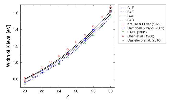
Figure 1: (Color online) Level widths of $K^{-1}$ hole state atomic level for atoms with 20$\leq$Z$\leq$30 compared to available theoretical and semi-empirical literature data: Krause and Oliver Krause and Oliver (1979), Campbell and Papp Campbell and Papp (2001), EADL Perkins et al. (1991), Chen et al. Chen et al. (1980), Casteleiro et al. Casteleiro et al. (2010).

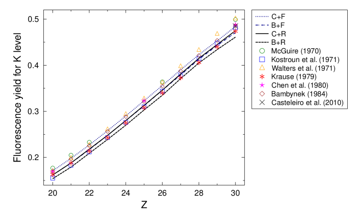
Figure 2: (Color online) Fluorescence yields of $K^{-1}$ hole state atomic level for atoms with 20$\leq$Z$\leq$30 compared to available theoretical and semi-empirical literature data: McGuire McGuire (1970), Kostroun et al. Kostroun et al. (1971), Walters et al. Walters and Bhalla (1971), Krause Krause (1979), Chen et al. Chen et al. (1980), Bambynek Bambynek (1984) (obtained from the compilation of Hubbell Hubbell et al. (1994)), Casteleiro et al. Casteleiro et al. (2010).

Table 7: Fluorescence yields of $K^{-1}$ hole state atomic level for atoms with 20$\leq$Z$\leq$30 compared to last obtained experimental literature data.

Z	Calculation model				Experimental data
	C+R	B+R	C+F	B+F	Yashoda et al.	Durak and Özdemır	Gudennavar et al.	Şimşek et al.
					Yashoda et al. (2005)	Durak and Özdemır (2001)	Gudennavar et al. (2003)	Şimşek et al. (2000)
20	0.154	0.161	0.163	0.170	-	-	-	-
21	0.184	0.175	0.193	0.184	-	-	-	-
22	0.218	0.209	0.227	0.217	0.218 $\pm$ 0.008	-	-	0.214 $\pm$ 0.004
23	0.248	0.239	0.258	0.248	0.249 $\pm$ 0.009	-	-	0.240 $\pm$ 0.008
24	0.280	0.270	0.290	0.280	-	-	-	0.291 $\pm$ 0.006
25	0.313	0.303	0.323	0.312	-	0.354 $\pm$ 0.007	-	0.311 $\pm$ 0.008
26	0.345	0.335	0.356	0.345	-	0.330 $\pm$ 0.005	-	0.331 $\pm$ 0.012
27	0.381	0.371	0.389	0.379	0.375 $\pm$ 0.014	-	-	0.355 $\pm$ 0.011
28	0.414	0.404	0.422	0.412	0.408 $\pm$ 0.015	0.412 $\pm$ 0.015	-	0.448 $\pm$ 0.014
29	0.440	0.448	0.448	0.456	0.438 $\pm$ 0.016	0.412 $\pm$ 0.029	-	0.455 $\pm$ 0.015
30	0.470	0.478	0.480	0.487	0.471 $\pm$ 0.018	0.482 $\pm$ 0.032	0.464 $\pm$ 0.010	0.482 $\pm$ 0.022
Z	Calculation model				Experimental data
	C+R	B+R	C+F	B+F	Şahin et al.	Söğüt	Han et al.
					Şahin et al. (2005)	Söğüt (2010)	Han et al. (2007)
20	0.154	0.161	0.163	0.170	0.174 $\pm$ 0.021	-	-
21	0.184	0.175	0.193	0.184	-	-	-
22	0.218	0.209	0.227	0.217	0.222 $\pm$ 0.027	-	0.234 $\pm$ 0.019
23	0.248	0.239	0.258	0.248	0.261 $\pm$ 0.031	-	0.264 $\pm$ 0.021
24	0.280	0.270	0.290	0.280	-	0.265 $\pm$ 0.026	0.295 $\pm$ 0.024
25	0.313	0.303	0.323	0.312	-	0.297 $\pm$ 0.030	0.351 $\pm$ 0.028
26	0.345	0.335	0.356	0.345	-	0.366 $\pm$ 0.033	0.358 $\pm$ 0.029
27	0.381	0.371	0.389	0.379	-	0.391 $\pm$ 0.039	-
28	0.414	0.404	0.422	0.412	-	0.451 $\pm$ 0.045	0.435 $\pm$ 0.035
29	0.440	0.448	0.448	0.456	-	0.478 $\pm$ 0.047	0.452 $\pm$ 0.036
30	0.470	0.478	0.480	0.487	-	0.525 $\pm$ 0.050	0.477 $\pm$ 0.038

In Table 7 and Figure 3 the comparison between present calculated values of $K^{-1}$ fluorescence yields and the last years literature experimental data is presented. A good agreement between present calculated values and the other literature data is obtained, nevertheless, because of the significant differences in experimental data, it is hard to state which calculation model out of those mentioned above is closer fitted to experimental values of fluorescence yields. In order to obtain this statement, the residual variances (i.e. a sum of squared residuals divided by a number of considered experimental points) for experimental points and theoretical points of four models have been calculated. These variances are collected in Table 8. From Tables 7 and 8, one can see that the experimental fluorescence yields presented in the papers of Yashoda et al. Yashoda et al. (2005), Durak and Özdemır Durak and Özdemır (2001), and Gudennavar et al. Gudennavar et al. (2003) are closer the theoretical values obtained by C+R model, the ones presented in the papers of Şimşek et al. Şimşek et al. (2000) and Söğüt Söğüt (2010) are closer to B+F model, and finally, these presented in the papers of Şahin et al. Şahin et al. (2005) and Han et al. Han et al. (2007) are closer to C+F model. However, the experimental fluorescence yields obtained with the smallest error, i.e. Yashoda et al. Yashoda et al. (2005) and Gudennavar et al. Gudennavar et al. (2003) data, are very close to the theoretical values obtained by C+R model. This would suggest that relativistic calculations based on both MCDF-originated radiative and non-radiative transition rates reproduce experimental fluorescence yields values better.

Table 8: Residual variances for experimental points and theoretical points of four models. All numbers are multiplied by $10^{4}$, e.g. 1.225 means 1.225$\times 10^{-4}$.

	Yashoda et al.	Durak and Özdemır	Gudennavar et al.	Şimşek et al.	Şahin et al.	Söğüt	Han et al.
Model	Yashoda et al. (2005)	Durak and Özdemır (2001)	Gudennavar et al. (2003)	Şimşek et al. (2000)	Şahin et al. (2005)	Söğüt (2010)	Han et al. (2007)
C+R	0.130	5.676	0.360	2.891	1.970	9.800	3.730
B+R	0.603	8.004	1.960	3.116	2.706	9.629	7.107
C+F	1.225	6.074	2.560	3.498	0.551	7.387	1.365
B+F	1.023	7.900	5.290	2.543	0.676	6.406	3.881

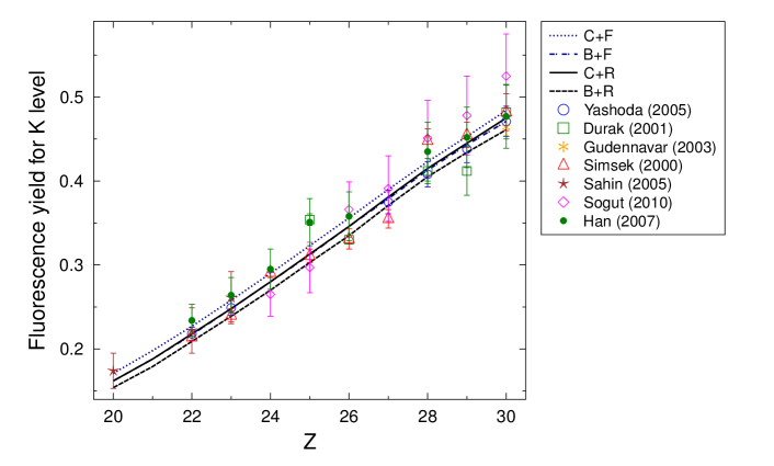
Figure 3: (Color online) Fluorescence yields of $K^{-1}$ hole state atomic level for atoms with 20$\leq$Z$\leq$30 compared to last obtained experimental literature data: Yashoda et al. Yashoda et al. (2005), Durak and Özdemır Durak and Özdemır (2001), Gudennavar et al. Gudennavar et al. (2003), Şimşek et al. Şimşek et al. (2000), Şahin et al. Şahin et al. (2005), Söğüt Söğüt (2010), Han et al. Han et al. (2007).

IV Conclusions

The $K$-shell level widths and $K$-shell fluorescence yields for atoms with 20$\leq$Z$\leq$30 have been calculated in relativistic way using MCDF and DHS calculations. The comparison between experimental fluorescence yields and theoretical ones, calculated by means of four models, results in satisfactory agreement. The present obtained results can be helpful in interpretation of experimental data of fluorescence yields and $K$-shell X-ray lines widths.

Acknowledgments

The Author is thankful to Gustavo Aucar (Northeastern University of Argentina) for hosting during this paper was being prepared.

References

- McGuire (1969) E. J. McGuire, Phys. Rev. A 85, 1 (1969).
- McGuire (1970) E. J. McGuire, Phys. Rev. A 2, 273 (1970).
- Walters and Bhalla (1971) D. L. Walters and C. P. Bhalla, Phys. Rev. A 3, 1919 (1971).
- Kostroun et al. (1971) V. O. Kostroun, M. H. Chen, and B. Craseman, Phys. Rev. A 3, 533 (1971).
- Bambynek et al. (1972) W. Bambynek, B. Crasemann, R.W. Fink, H.U. Freund, H. Mark, C.D. Swift, R.E. Price, and P.V. Rao, Rev. Mod. Phys. 44, 716 (1972).
- Krause and Oliver (1979) M. O. Krause and J. H. Oliver, J. Phys. Chem. Ref. Data 8, 329 (1979).
- Krause (1979) M. O. Krause, J. Phys. Chem. Ref. Data 8, 307 (1979).
- Chen et al. (1980) M. H. Chen, B. Crasemann, and H. Mark, Phys. Rev. A 21, 436 (1980).
- Hubbell et al. (1994) J. H. Hubbell, P. N. Trehan, N. Singh, B. Chand, D. Mehta, M. L. Garg, R. R. Garg, S. Singh, and S. Puri, J. Phys. Chem. Ref. Data 23, 339 (1994).
- Campbell and Papp (2001) J. L. Campbell and T. Papp, Atomic Data and Nuclear Data Tables 77, 1 (2001).
- Perkins et al. (1991) S. T. Perkins, D. E. Cullen, M.-H. Chen, J. H. Hubbell, J. Rathkopf, and J. H. Scofield, Tech. Rep. UCRL-50400 30, Lawrence Livermore National Laboratory (1991).
- Polasik et al. (2011) M. Polasik, K. Słabkowska, J. Rzadkiewicz, K. Kozioł, J. Starosta, E. Wiatrowska-Kozioł, J.-Cl. Dousse, and J. Hoszowska, Phys. Rev. Lett. 107, 073001 (2011).
- Yashoda et al. (2005) T. Yashoda, S. Krishnaveni, and R. Gowda, Nucl. Instru. Meth. Phys. B 240, 607 (2005).
- Şahin et al. (2005) M. Şahin, L. Demir, and G. Budak, Appl. Radiat. Isot. 63, 141 (2005).
- Gudennavar et al. (2003) S.B. Gudennavar, N.M. Badiger, S.R. Thontadarya, and B. Hanumaiah, Rad. Phys. and Chem. 68, 721 (2003).
- Durak and Özdemır (2001) R. Durak and Y. Özdemır, Rad. Phys. Chem. 61, 19 (2001).
- Şimşek et al. (2000) Ö. Şimşek, O. Doğan, Ü. Turgut, and M. Ertuğrul, Rad. Phys. Chem. 58, 207 (2000).
- Söğüt (2010) Ö. Söğüt, Chin. J. Phys. 48, 212 (2010).
- Han et al. (2007) I. Han, M. Şahin, L. Demir, and Y. Şahin, Appl. Radiat. Isot. 65, 669 (2007).
- Grant et al. (1980a) I. P. Grant, B. J. McKenzie, P. H. Norrington, D. F. Mayers, and N.C. Pyper, Comput. Phys. Commun. 21, 207 (1980a).
- Grant et al. (1980b) I. P. Grant, B. J. McKenzie, and P. H. Norrington, Comput. Phys. Commun. 21, 233 (1980b).
- Grant and J.McKenzie (1980) I. P. Grant and B. J.McKenzie, J. Phys. B 13, 2671 (1980).
- Hata and Grant (1983) J. Hata and I.P. Grant, J. Phys. B 16, 3713 (1983).
- Grant (1984) I.P. Grant, Int. J. Quantum Chem. 25, 23 (1984).
- Dyall et al. (1989) K. G. Dyall, I. P. Grant, C. T. Johonson, F. A. Parpia, and E. P. Plummer, Comput. Phys. Commun. 55, 425 (1989).
- Grant (1974) I.P. Grant, J. Phys. B 7, 1458 (1974).
- Grant (1988) I.P. Grant, Relativistic Effects in Atoms and Molecules, in: Methods in Computational Chemistry, vol. 2 (Plenum, New York, 1988).
- Polasik (1989) M. Polasik, Phys. Rev. A 39, 616 (1989).
- Polasik (1995) M. Polasik, Phys. Rev. A 52, 227 (1995).
- Gu (2008) M. F. Gu, Can. J. Phys. 86, 675 (2008).
- Jönsson et al. (2007) P. Jönsson, X. He, C. Froese Fischer, and I.P. Grant, Comput. Phys. Commun. 177, 597 (2007).
- Babushkin (1964) F. A. Babushkin, Acta Phys. Polon. 25, 749 (1964).
- Gu (2003) M. F. Gu, Astrophys. J. 582, 1241 (2003).
- Fritzsche (2001) S. Fritzsche, J. Elect. Spect. Rel. Phen. 114, 1155 (2001).
- Fritzsche (2012) S. Fritzsche, Comput. Phys. Commun. 183, 1525 (2012).
- Parpia et al. (1996) F. A. Parpia, C. Froese Fischer, and I. P. Grant, Comput. Phys. Commun. 94, 249 (1996).
- Casteleiro et al. (2010) C. Casteleiro, F. Parente, P. Indelicato, and J. P. Marques, Eur. Phys. J. D 56, 1 (2010).
- Bambynek (1984) W. Bambynek, A New Evaluation of K-Shell Fluorescence Yields (X-84 Proc., Leipzig, 1984).