A Hardware-aware and Stable Orthogonalization Framework

Abstract

The orthogonalization process is an essential building block in Krylov space methods, which takes up a large portion of the computational time. Commonly used methods, like the Gram-Schmidt method, consider the projection and normalization separately and store the orthogonal base explicitly. We consider the problem of orthogonalization and normalization as a QR decomposition problem on which we apply known algorithms, namely CholeskyQR and TSQR. This leads to methods that solve the orthogonlization problem with reduced communication costs, while maintaining stability and stores the orthogonal base in a locally orthogonal representation. Furthermore, we discuss the novel method as a framework which allows us to combine different orthogonalization algorithms and use the best algorithm for each part of the hardware. After the formulation of the methods, we show their advantageous performance properties based on a performance model that takes data transfers within compute nodes as well as message passing between compute nodes into account. The theoretic results are validated by numerical experiments.

15A23, 65F25, 65Y05

1 Introduction

The orthogonalization process is an important building block in Krylov space methods, both to solve linear systems as well as to compute eigenvectors. In this paper we focus on the orthogonalization as part of the Arnoldi process, as it is used for example in the GMRes method. Beside the application of the operator (and the preconditioner) the projection and orthogonalization step takes up the major portion of the runtime. On modern architectures not the actual computation is the bottleneck, but communication [9]. Communication means the exchange of data between the components of the hardware. This exchange happens between the memory and the CPU as well as between compute nodes in distributed environments. This paper aims at algorithms that optimize the communication and hence achieve better performance in high-performance computing (HPC) environments. To this end, we extend the TSQR algorithm [7, 8] and adopt the data structure to store the base of the Krylov space in a locally orthogonal representation. Based on it we introduce a framework in which different algorithms can be combined utilizing their advantages on different parts of the computer architecture.

Communication-avoiding and communication-hiding Krylov methods gained a lot attention these days. In particular Block Krylov methods are well suited for high-performance computing [11, 10]. These methods were originally developed to solve linear systems with multiple right-hand sides [18] or to compute multiple eigenvectors simultaneously [14]. Since then also block variants of the Arnoldi method [19] and GMRes method [21] were proposed.

A particular issue of the orthogonalization process is stability. Especially the classical Gram-Schmidt procedure may produce a significant orthogonalization error. The stability properties of various block Gram-Schmidt procedures are analyzed in the paper of Carson et al. [4] and an excellent overview of existing block Gram-Schmidt methods is given in [5], taking performance and stability into account.

A new approach for reducing the synchronization cost in a block Gram-Schmidt algorithm are presented by Swirydowicz et al. [23]. To remedy the problem of synchronization points in the block Gram-Schmidt process, they propose the so-called low-synch [23, 3] methods that delay the normalization of Krylov vectors.

Yamazaki et al. [28] already presented a method that combines the projection and normalization step in a single reduction in the context of the classical Gram-Schmidt method. This was later extended to block Gram-Schmidt [5] under the name BCGS-PIP. The same algorithm can be derived in our setting as we will see in Section 3.

The separate consideration of projection and normalization leads to multiple synchronization points, at least two. This paper is based on the observation, that these problems can be treated together: Let $Q\in\mathbb{R}^{n\times k}$ be an orthogonal matrix which columns span the already computed Krylov space and $X\in\mathbb{R}^{n\times s}$ the block-vector that contains the new directions of the Krylov space. The aim is now to compute an orthogonal matrix $U\in\mathbb{R}^{n\times t}$ such that $\operatorname{span}(Q,U)=\operatorname{span}(Q,X)$ and $Q^{T}U=0$. We call this problem the project and normalize (PQR) problem. It can be solved by computing the reduced QR factorization

(1) $$\begin{bmatrix}Q&X\end{bmatrix} =\begin{bmatrix}Q&U\end{bmatrix}\begin{bmatrix}I&P\\ 0&N\end{bmatrix},$$

with projection matrix $P\in\mathbb{R}^{k\times s}$ and normalizer $N\in\mathbb{R}^{t\times s}$. In most cases we have $t=s$ and $N$ is a upper triangular matrix. The other case, $t<s$, appears if the system $\begin{bmatrix}Q&X\end{bmatrix}$ is linearly dependent. In the context of block Krylov space methods this case is called the deflation case. The matrix $N$ is then a row-echelon matrix. Depending on the implementation details, it might be reasonable to use $t=s$ in all cases and treat the rank-deficiency of $N$ later on. One possibility is to use a rank-revealing QR-decomposition, i.e. pivoting, to enforce triangular shape of $N$.

The matrix $Q$ must not necessarily stored explicitly, but, depending on the orthogonlization method, it might be useful to store it in an other representation. Walker [25] for example used a sequence of Householder reflectors to store the orthogonal base in the GMRes method. This was proposed by Walker [25]. In Section 4 we will use a locally orthogonal representation. However, the output $U$ of the method should be available explicitly, as it used to compute the subsequent Krylov space directions by applying the operator.

Computing the QR-factorization (1) is actually more costly than the original orthogonalization problem, but as we know QR-factorization algorithms (namely CholQR [15, Thm. 5.2.3] and TSQR [8]) that can solve this problem with only one global synchronization, we can apply these algorithm to solve the projection and normalize problem with one global synchronization. Additionally, we can make use of the known structure of problem (1), i.e. $Q$ is already orthogonal, to simplify and improve the resulting method.

The main contribution of this paper is an orthogonalization framework for Krylov methods so, that the actual algorithm can be adapted to the properties of the hardware. It is structured as follows. In Section 2 we show how a method that solves problem (1) can be used in the Arnoldi procedure and review the Gram-Schmidt and Householder method for the orthogonalization. These methods are the fundamental building blocks in the framework. As a further building block we discuss the BCGS-PIP method, and show how to deduce it from the Cholesky QR algorithm in Section 3. In the same manner we introduce the novel TreeTSPQR and FlatTSPQR methods, which are deduced from the respective TSQR algorithm in Section 4, which act as connectors between the building blocks. In Section 5 we use performance models to analyze the performance of the different algorithms and show how the TSPQR algorithms can be combined with the Householder and BCGS-PIP+ method to build an orthogonalization framework that is adapted on the architecture of a given supercomputer. Numerical experiments that show the stability and performance properties are given in Section 6. Finally, we give a conclusion and outlook in Section 7.

2 Orthogonalization in Krylov space methods

Let $R\in\mathbb{R}^{n\times s}$ with ${s\ll n}$. The block Arnoldi method constructs a sequence of orthogonal bases $\mathcal{V}_{k}$ for the block Krylov space

(2) $$\mathcal{K}^{k}(A,R) =\operatorname{span}\left(R,AR,\ldots,A^{k-1}R\right)$$

and block-Hessenberg matrices $H_{k}$ that satisfy the so-called block Arnoldi relation

(3) $$A\mathcal{V}_{k-1}=\mathcal{V}_{k}H_{k}.$$

The algorithm can be formulated by solving problem (1) in every iteration. The algorithm is shown in Algorithm 1.

Algorithm 1 Block Arnoldi

$V_{0}=RH_{0}$$\triangleright$ QR-factorization

for $i=0,\ldots$ do

     $X_{i+1}=AV_{i}$

     $\begin{bmatrix}\mathcal{V}_{i}&X_{i+1}\end{bmatrix}=\begin{bmatrix}\mathcal{V}_{i}&V_{i+1}\end{bmatrix}\begin{bmatrix}I&P\\ 0&N\end{bmatrix}$ $\triangleright$ Solve (1)

     $\mathcal{V}_{i+1}=\begin{bmatrix}\mathcal{V}_{i}&V_{i+1}\end{bmatrix}$

     $H_{i+1}=\begin{bmatrix}H_{i}&P\\ 0&N\end{bmatrix}$

end for

The basis $\mathcal{V}_{k}$ can then be used in the block GMRes method to solve large sparse linear systems with multiple right-hand sides or to compute eigenvectors of the operator $A$. The spectrum of $H_{k}$ is an approximation for the spectrum of $A$.

In practice two strategies are commonly used to solve (1) in Algorithm 1. The Gram-Schmidt method, either in the classical or in the modified variant, and the Householder method. Depending on the used orthogonalization method the matrices $\mathcal{V}_{k}$ might not be stored explicitly. As we will see, if the Householder method is used, the basis $\mathcal{V}_{k}$ is stored as product of Householder reflectors. Similarly, in the method introduced in Section 4 it is stored as the product of locally orthogonal matrices.

To assess the stability of the presented algorithms we apply them for computing a QR-factorization of a matrix $A$. Algorithm 2 computes the QR-factorization by solving the PQR problem (1) block-column-wise, where $A_{i}$ denote the $i$th block-column of $A$ i.e. the columns $si$ to $s(i+1)$.

Algorithm 2 Block Column-oriented QR-factorization

$A_{0}=Q_{0}R_{0}$ $\triangleright$ QR-factorization

for $i=1\,\ldots\,\frac{m}{s}$ do

     $\begin{bmatrix}Q_{i}&A_{i+1}\end{bmatrix}=\begin{bmatrix}Q_{i}&U_{u}\end{bmatrix}\begin{bmatrix}I&P\\ 0&N\end{bmatrix}$ $\triangleright$ Solve (1)

     $Q_{i+1}=\begin{bmatrix}Q_{i}&U_{i}\end{bmatrix}$

     $R_{i}=\begin{bmatrix}R_{i-1}&P\\ 0&N\end{bmatrix}$

end for

The orthogonality error in the Frobenius norm

(4) $$e_{\perp}:=\|I-Q^{T}Q\|_{F}$$

gives an indication for the stability, as accumulated errors immediately impede the orthogonality and increase the error $e_{\perp}$. Estimations for $e_{\perp}$ are given depended on the machine precision and condition number of the input matrix $A$, cf. Section 6. We will denote the machine precision by $\varepsilon$ and the condition number by $\kappa$.

2.1 Gram-Schmidt

The Gram-Schmidt method is the oldest variant for orthogonalizing a set for vectors. The block classical variant (BCGS) projects the matrix $X$ onto the orthogonal complement of $Q$ by computing

(5) $$\tilde{U}=(I-QQ^{T})X=X-Q(Q^{T}X).$$

After that the result is normalized by computing the reduced QR decomposition of $\tilde{U}$. This QR factorization can for example be efficiently computed by the TSQR algorithm or by the CholQR algorithm. The resulting algorithm is shown in Algorithm 3.

Algorithm 3 Block Classical Gram-Schmidt (BCGS)

$P=Q^{T}X$

$\tilde{U}=X-QP$

$\tilde{U}=UN$ $\triangleright$ QR factorization

As shown by Giraud et al. [13] the orthogonalization error of the BCGS method is of order $\mathcal{O}(\varepsilon\kappa^{2})$.

To improve the stability the modified Gram-Schmidt method was introduced and adapted for block orthogonalization [17]. It computes the projection of each column $q_{i}$ in $Q$ separately

(6) $$\tilde{U}=(I-q_{k}q_{k}^{T})\cdots(I-q_{1}q_{1}^{T})X.$$

This leads to an orthogonalization error of $\mathcal{O}(\varepsilon\kappa)$. Algorithm 4 shows the pseudocode of the algorithm. Subscripts denote the column of the respective matrix.

Algorithm 4 Block Modified Gram-Schmidt (BMGS)

$\tilde{U}_{0}=X$

for $i=1,\ldots,k$ do

     $P_{i}=q_{i}^{T}\tilde{U}_{i-1}$

     $\tilde{U}_{i}=\tilde{U}_{i-1}-q_{i}P_{i}$

end for

$\tilde{U}_{k}=UN$$\triangleright$ QR factorization

The modified Gram-Schmidt method has the disadvantage that $k$ inner products are computed sequentially. In contrast to the classical variant this means that the matrix $U$ is loaded $k$ times from the memory and in a distributed computation environment this leads to $k$ collective communications, i.e. synchronization points.

Another approach for improving the stability is the reiteration of the classical Gram-Schmidt method [1]. It improves the orthogonalization error of the classical Gram-Schmidt method by applying the algorithm twice. It is proven that the first reiteration brings the orthogonalization error down to $\mathcal{O}(\varepsilon)$ [2]. Algorithm 5 shows the reiterated BCGS algorithm (BCGS+). As the BCGS method is applied twice, the costs for the BCGS+ method are twice the costs for the BCGS method.

Algorithm 5 Block Classical Gram-Schmidt with reiteration (BCGS+)

Solve $\begin{bmatrix}Q&X\end{bmatrix}=\begin{bmatrix}Q&U_{1}\end{bmatrix}\begin{bmatrix}I&P_{1}\\ 0&N_{1}\end{bmatrix}$ using BCGS

Solve $\begin{bmatrix}Q&U_{1}\end{bmatrix}=\begin{bmatrix}Q&U\end{bmatrix}\begin{bmatrix}I&P_{2}\\ 0&N_{2}\end{bmatrix}$ using BCGS

$P=P_{1}N_{2}+P_{2}$ and $N=N_{2}+N_{1}N_{2}$

2.2 Householder

We consider the Householder method in a form that treats the problem column-wise, an elaborate analysis can be found in the book of Golub and von Loan [15, Chapter 5]. For brevity we employ a python-style slicing syntax to refer to submatrices and subvectors. It is indicated by rectangular brackets. E.g. $X\texttt{[}\StrSubstitute{0:k}{:}{\,\mathtt{:}\,},\StrSubstitute{i}{:}{\,\mathtt{:}\,}\texttt{]}$ denotes the first $k$ entries of the $i$th column of $X$.

The matrix $Q$ in the Householder method is stored as a product of Householder reflectors

(7) $$\mathcal{Q}_{k} =H_{0}\cdots H_{k-1} H_{i}=I-2v_{i}v_{i}^{T},$$ with

for some $v_{i}\in\mathbb{R}^{n}$ with $\|v_{i}\|=1$. The operators $H_{i}$ are symmetric and orthogonal. The matrix $Q$ can be explicitly assembled by applying the operator $\mathcal{Q}_{k}$ to the first $k$ unit vectors

(8) $$Q=\mathcal{Q}_{k}I\texttt{[}\StrSubstitute{0:n}{:}{\,\mathtt{:}\,},\StrSubstitute{0:k}{:}{\,\mathtt{:}\,}\texttt{]}.$$

To solve problem (1), the new Householder reflectors are constructed column by column. Let $\mathcal{Q}_{k+i}=H_{0}\cdots H_{k+i-1}$ be constructed. The next column $X\texttt{[}\StrSubstitute{0:n}{:}{\,\mathtt{:}\,},\StrSubstitute{i}{:}{\,\mathtt{:}\,}\texttt{]}$ in $X$ is projected by applying $\mathcal{Q}^{T}_{k+i}$

(9) $$\tilde{u}_{i}=\mathcal{Q}_{k+i}^{T}X\texttt{[}\StrSubstitute{0:n}{:}{\,\mathtt{:}\,},\StrSubstitute{i}{:}{\,\mathtt{:}\,}\texttt{]}=H_{k+i-1}\cdots H_{0}X\texttt{[}\StrSubstitute{0:n}{:}{\,\mathtt{:}\,},\StrSubstitute{i}{:}{\,\mathtt{:}\,}\texttt{]}.$$

The upper $k$ entries in $\tilde{u}_{i}$ are the respective coefficients of $P$ and $N$

(10) $$P\texttt{[}\StrSubstitute{0:n}{:}{\,\mathtt{:}\,},\StrSubstitute{i}{:}{\,\mathtt{:}\,}\texttt{]} =\tilde{u}_{i}\texttt{[}\StrSubstitute{0:k}{:}{\,\mathtt{:}\,}\texttt{]} N\texttt{[}\StrSubstitute{0:i}{:}{\,\mathtt{:}\,},\StrSubstitute{i}{:}{\,\mathtt{:}\,}\texttt{]}=\tilde{u}_{i}\texttt{[}\StrSubstitute{k:k\!+\!i}{:}{\,\mathtt{:}\,}\texttt{]}.$$

From the lower part the vector $\tilde{v}_{k}$ is computed as

(11) $$\tilde{v}_{k}=(\tilde{u}\texttt{[}\StrSubstitute{k\!+\!i:n}{:}{\,\mathtt{:}\,}\texttt{]}-\sigma\lambda e_{1}),$$

where $\lambda$ is the norm of the lower part of $\tilde{u}$ and $\sigma$ chosen as the invert sign of $\tilde{u}\texttt{[}\StrSubstitute{k}{:}{\,\mathtt{:}\,}\texttt{]}$ to avoid cancellation and improve the stability of the algorithm. The diagonal entry of $N$ is then given by $N\texttt{[}\StrSubstitute{i}{:}{\,\mathtt{:}\,},\StrSubstitute{i}{:}{\,\mathtt{:}\,}\texttt{]}=\sigma\lambda$. This vector is then normalized to obtain the Householder reflector

(12) $$v_{k+1}\texttt{[}\StrSubstitute{k:n}{:}{\,\mathtt{:}\,}\texttt{]}=\frac{1}{\|\tilde{v}_{k+1}\|}\tilde{v}_{k+1},$$

while the upper $k$ coefficients are set to $0$.

Algorithm 6 Householder (HH)

1:$\tilde{X}=H_{k-1}\cdots H_{0}X$

2:for $i=0\ldots s-1$ do

3:     $\tilde{u}_{i}=H_{k+i-1}\cdots H_{k}\tilde{X}\texttt{[}\StrSubstitute{0:n}{:}{\,\mathtt{:}\,},\StrSubstitute{i}{:}{\,\mathtt{:}\,}\texttt{]}$

4:     $P\texttt{[}\StrSubstitute{0:n}{:}{\,\mathtt{:}\,},\StrSubstitute{i}{:}{\,\mathtt{:}\,}\texttt{]}=\tilde{u}_{i}\texttt{[}\StrSubstitute{0:k}{:}{\,\mathtt{:}\,},\StrSubstitute{i}{:}{\,\mathtt{:}\,}\texttt{]}$

5:     $N\texttt{[}\StrSubstitute{0:i}{:}{\,\mathtt{:}\,},\StrSubstitute{i}{:}{\,\mathtt{:}\,}\texttt{]}=\tilde{u}_{i}\texttt{[}\StrSubstitute{k:k\!+\!i}{:}{\,\mathtt{:}\,},\StrSubstitute{i}{:}{\,\mathtt{:}\,}\texttt{]}$

6:     $\lambda=\|\tilde{u}_{i}\texttt{[}\StrSubstitute{k:n}{:}{\,\mathtt{:}\,},\StrSubstitute{i}{:}{\,\mathtt{:}\,}\texttt{]}\|_{2}$

7:     $\sigma=-\operatorname{sgn}(\tilde{u}_{i}\texttt{[}\StrSubstitute{k}{:}{\,\mathtt{:}\,},\StrSubstitute{i}{:}{\,\mathtt{:}\,}\texttt{]})$

8:     $N\texttt{[}\StrSubstitute{i}{:}{\,\mathtt{:}\,},\StrSubstitute{i}{:}{\,\mathtt{:}\,}\texttt{]}=\sigma\lambda$

9:     $\tilde{v}_{k+i}=\tilde{u}\texttt{[}\StrSubstitute{k\!+\!i:n}{:}{\,\mathtt{:}\,},\StrSubstitute{i}{:}{\,\mathtt{:}\,}\texttt{]}-\sigma\lambda e_{1}$

10:     $v_{k+i}\texttt{[}\StrSubstitute{k\!+\!i:n}{:}{\,\mathtt{:}\,}\texttt{]}=\frac{1}{\|\tilde{v}_{k+i}\|}\tilde{v}_{k+i}$

11:end for

Algorithm 6 shows the pseudocode for the Householder method (HH). In practice the application of the Householder reflectors $H_{k-1}\cdots H_{0}$ can be applied on block for all columns in $X$. This avoids reading $v_{k}\ldots v_{1}$ from the memory in every loop iteration. The algorithm is known to be stable and produces and orthogonalization error in $\mathcal{O}(\varepsilon)$.

3 BCGS-PIP

The CholQR algorithm is a well-known algorithm for computing the QR factorization of a tall-skinny matrix. It computes the QR factorization of a matrix $A$ by Cholesky factorizing the Gram matrix $A^{T}A=LL^{T}$. The QR factorization is then given by $A=QR$ with $Q=XL^{-T}$ and $R=L^{T}$. While this algorithm has optimal performance properties, it renders unstable if the matrix $A$ is ill-conditioned. As it was shown by Carson et al. [4] and we will also see in Section 6 the orthogonalization error is of order $\mathcal{O}(\kappa^{2}\varepsilon)$, as long as $\kappa^{2}<\varepsilon^{-1}$.

To deduce the algorithm, we apply the Cholesky QR algorithm on the PQR problem (1). The occurring Gram matrix can be Cholesky factorized by

(13) $$\begin{bmatrix}Q&X\end{bmatrix}^{T}\begin{bmatrix}Q&X\end{bmatrix} =\begin{bmatrix}I&P\\ P^{T}&X^{T}X\end{bmatrix}$$

(14) $$=\begin{bmatrix}I&0\\ P^{T}&N^{T}\end{bmatrix}\begin{bmatrix}I&P\\ 0&N\end{bmatrix},$$

where $P=Q^{T}X$ and $N$ is the Cholesky factor of $X^{T}X-P^{T}P=N^{T}N$. The result $U$ is then given by

(15) $$U=XL^{-T}-QPL^{-T}.$$

This algorithm is called BCGS-PIP [4]. The PIP stands for Pythagorean Inner Product and refers to the original derivation from the Pythagorean theorem. As it already holds for the CholQR algorithm, this algorithm turns out to be quite unstable. Like CholQR or BCGS, the orthogonlization error is of order $\mathcal{O}(\kappa^{2}\varepsilon)$. For a detailed stability analysis see [5]. The pseudocode for this algorithm is shown in Algorithm 7.

Algorithm 7 BCGS-PIP

Compute $P=Q^{T}X$ and $G=X^{T}X$ $\triangleright$ At once

Compute Cholesky factorization $N^{T}N=G-P^{T}P$

$U=XN^{-1}-QPN^{-1}$

Regarding the communication, the algorithm requires one synchronization for computing the Gram and projection matrix. The matrices $Q$ and $X$ are loaded two times from the memory, once for the computation of $G$ and $P$ and once for the assembly of $U$.

Using this algorithm in the GMRes method leads to the so-called one-step latency method presented by Ghysels et al. [12].

3.1 Reiteration

A remedy for the loss of orthogonalization is to reiterate the algorithm [27]. As for the BCGS+ method, this brings the orthogonalization error down to machine precision as long as $\varepsilon\kappa^{2}\leq\frac{1}{2}$, while doubling the computational and communication effort. In total this algorithm performs two synchronizations and loads the matrices $Q$ and $X$ four times. BCGS-PIP with reiteration (BCGS-PIP+) is shown in Algorithm 8.

Algorithm 8 BCGS-PIP with reiteration (BCGS-PIP+)

Compute $P_{1}=Q^{T}X$ and $G_{1}=X^{T}X$ $\triangleright$ At once

Compute Cholesky factorization $N_{1}^{T}N_{1}=G_{1}-P_{1}^{T}P_{1}$

$U_{1}=XN_{1}^{-1}-QP_{1}N_{1}^{-1}$

Compute $P_{2}=Q^{T}U_{1}$ and $G_{2}=U_{1}^{T}U_{1}$ $\triangleright$ At once

Compute Cholesky factorization $N_{2}^{T}N_{2}=G_{2}-P_{2}^{T}P_{2}$

$U=U_{1}N_{2}^{-1}-QP_{2}N_{2}^{-1}$

$P=P_{1}N_{2}+P_{2}$ and $N=N_{2}+N_{1}N_{2}$

Another drawback of the algorithm is the implementation of deflation. The textbook variant of the Cholesky factorization is not rank-revealing, meaning it can not be used to decide whether $G$ has full rank. Hence we perform a singular value-decomposition of the matrix $G-P^{T}P=U\Sigma U^{T}$, where we truncate singular values smaller than a certain tolerance, yielding a full-rank square-root

(16) $$N=\tilde{U}\tilde{\Sigma}^{\frac{1}{2}}$$

of $G-P^{T}P$, where $\tilde{\Sigma}$ denotes the diagonal matrix of the significant singular values and $\tilde{U}$ the corresponded left columns of $U$.

4 TSPQR

After we have introduced several orthogonalization methods, we now propose the TSPQR method. It subdivides the PQR problem into smaller problems of the same type and thus enables us to apply recursion. Furthermore, it builds up on the previous introduced methods and gives us the choice which method is used on which level.

Like the BCGS-PIP algorithm the TSPQR algorithm is derived from the QR-factorization problem (1), but instead of the CholQR algorithm, we apply the TSQR algorithm [8]. It was proposed in two variants - a tree reduction and a sequential incremental one. We will consider both in the following subsections.

4.1 TreeTSPQR

The tree-TSQR algorithm computes a QR factorization of a tall-skinny matrix $A\in\mathbb{R}^{n\times s}$ by row-wise decomposing $A$ into $p$ local blocks and factorizing these blocks in parallel

(17) $$A=\begin{bmatrix}A_{1}\\ \vdots\\ A_{p}\end{bmatrix}=\begin{bmatrix}Q_{1}R_{1}\\ \vdots\\ Q_{p}R_{p}\end{bmatrix}.$$

The word local emphasizes that the problems are so small that they can be solved without communication.

Then, the QR factorization of the vertically stacked $R$-factors is computed

(18) $$\begin{bmatrix}R_{1}\\ \vdots\\ R_{p}\end{bmatrix}=\begin{bmatrix}S_{1}\\ \vdots\\ S_{p}\end{bmatrix}R$$

and the global QR factorization of $A$ is then given by

(19) $$A=\begin{bmatrix}Q_{1}S_{1}\\ \vdots\\ Q_{p}S_{p}\end{bmatrix}R.$$

To avoid that the QR factorization of the $R$-factors grows to large and thus become too costly, this algorithm is applied recursively, meaning it is applied itself to compute the local QR factorizations in equation (17), or to compute the reduced QR factorization (18).

Now we apply the TSQR algorithm to compute the factorization (1). For that we assume that the matrix $Q$ was also computed with this algorithm and is therefore stored in the TSQR representation, i.e.

(20) $$Q=\begin{bmatrix}Q_{1}\\ &Q_{2}\\ &&\ddots\\ &&&Q_{p}\end{bmatrix}\begin{bmatrix}R_{1}\\ R_{2}\\ \vdots\\ R_{p}\end{bmatrix},$$

where $Q_{1},\ldots,Q_{p}$ are local orthogonal matrices and $R_{1},\ldots,R_{p}$ are local upper triangular matrices. As the matrix $Q$ is orthogonal we see that the stacked matrix of $R$-factors is orthogonal too

(21) $$\begin{bmatrix}R_{1}^{T},\ldots,R_{p}^{T}\end{bmatrix}\begin{bmatrix}R_{1}\\ \vdots\\ R_{p}\end{bmatrix} =\begin{bmatrix}R_{1}^{T},\ldots,R_{p}^{T}\end{bmatrix}\begin{bmatrix}Q_{1}^{T}\\ &\ddots\\ &&Q_{p}^{T}\end{bmatrix}\begin{bmatrix}Q_{1}\\ &\ddots\\ &&Q_{p}\end{bmatrix}\begin{bmatrix}R_{1}\\ \vdots\\ R_{p}\end{bmatrix}$$

(22) $$=Q^{T}Q$$

(23) $$=I.$$

Applying the TSQR algorithm on problem (1) then means that we first must solve the local QR factorizations

(24) $$\begin{bmatrix}Q_{i}R_{i}&X_{i}\end{bmatrix} =\begin{bmatrix}Q_{i}&U_{i}\end{bmatrix}\begin{bmatrix}R_{i}&P_{i}\\ 0&N_{i}\end{bmatrix}$$

for every $i=1\ldots,p$, which is equivalent to

(25) $$\begin{bmatrix}Q_{i}&X_{i}\end{bmatrix} =\begin{bmatrix}Q_{i}&U_{i}\end{bmatrix}\begin{bmatrix}I&P_{i}\\ 0&N_{i}\end{bmatrix}.$$

This problem is the same as (1) but of smaller size and can be solved locally by one of the previous mentioned methods (or by a TSPQR algorithm itself to introduce recursion). We call the algorithm that is used for solving these problems the local subalgorithm.

Once all the local problems are solved, a reduction step computes the QR factorization of the stacked $R$ factors:

(26) $$\begin{bmatrix}R_{1}&P_{1}\\ 0&N_{1}\\ \vdots&\vdots\\ R_{p}&P_{p}\\ 0&N_{p}\\ \end{bmatrix} =\begin{bmatrix}R_{1}&\widetilde{P}_{1}\\ 0&\widetilde{N}_{1}\\ \vdots\\ R_{p}&\widetilde{P}_{p}\\ 0&\widetilde{N}_{p}\\ \end{bmatrix}\begin{bmatrix}I&P\\ 0&N\end{bmatrix},$$

which is again a variant of problem (1), as we have seen that the stacked R-factors are orthogonal. The algorithm that is used to solve this problem is called the reduction subalgorithm.

The solution of the global system is then given by

(27) $$\begin{bmatrix}Q&X\end{bmatrix} =\begin{bmatrix}\begin{bmatrix}Q_{1}&U_{1}\end{bmatrix}\begin{bmatrix}R_{1}&\widetilde{P}_{1}\\ 0&\widetilde{N}_{1}\end{bmatrix}\\ \vdots\\ \begin{bmatrix}Q_{p}&U_{p}\end{bmatrix}\begin{bmatrix}R_{p}&\widetilde{P}_{p}\\ 0&\widetilde{N}_{p}\end{bmatrix}\\ \end{bmatrix}\begin{bmatrix}I&P\\ 0&N\end{bmatrix}.$$

The matrix $U$ can then be computed by block-wise matrix products

(28) $$U=\begin{bmatrix}\begin{bmatrix}Q_{1}&U_{1}\end{bmatrix}\begin{bmatrix}\widetilde{P}_{1}\\ \widetilde{N}_{1}\end{bmatrix}\\ \vdots\\ \begin{bmatrix}Q_{p}&U_{p}\end{bmatrix}\begin{bmatrix}\widetilde{P}_{p}\\ \widetilde{N}_{p}\end{bmatrix}\end{bmatrix}.$$

Algorithm 9 TreeTSPQR

for $i=1,\ldots,p$ do

     Solve $\begin{bmatrix}Q_{i}&X_{i}\end{bmatrix}=\begin{bmatrix}Q_{i}&U_{i}\end{bmatrix}\begin{bmatrix}I&P_{i}\\ &N_{i}\end{bmatrix}$

end for

Solve $\begin{bmatrix}R_{1}&P_{1}\\ &N_{1}\\ \vdots&\vdots\\ R_{p}&P_{p}\\ &N_{p}\end{bmatrix}=\begin{bmatrix}R_{1}&\widetilde{P}_{1}\\ &\widetilde{N}_{1}\\ \vdots&\vdots\\ R_{p}&\widetilde{P}_{p}\\ &\widetilde{N}_{p}\\ \end{bmatrix}\begin{bmatrix}R&P\\ &N\end{bmatrix}$

Algorithm 9 shows the pseudocode for the tree variant of the TSPQR algorithm (TreeTSPQR). As the local subproblems are independent they can be solved in parallel. The size of the subproblems should be chosen such that all data fits in the cache, so it must only be loaded once from the main memory. In Section 6 (Fig. 5) we show a benchmark regarding the size of the subproblems.

4.2 FlatTSPQR

There is also a flat variant of the TSQR algorithm that we apply on problem (1) as well, to derive a flat variant of the TSPQR algorithm. Flat TSQR computes a QR decomposition by factorizing the upper part of the matrix and proceed with the remainder stacked with the R-factor of the upper part

(29) $$A =\begin{bmatrix}Q_{1}R_{1}\\ A_{1}\end{bmatrix}=\begin{bmatrix}Q_{1}\\ &I\end{bmatrix}\begin{bmatrix}R_{1}\\ A_{1}\end{bmatrix}=\begin{bmatrix}Q_{1}\\ &I\end{bmatrix}\begin{bmatrix}Q_{2}\\ &I\end{bmatrix}\begin{bmatrix}R_{2}\\ A_{2}\end{bmatrix}=\ldots$$

$$=\begin{bmatrix}Q_{1}\\ &I\end{bmatrix}\cdots\begin{bmatrix}Q_{p-1}\\ &I\end{bmatrix}Q_{p}R.$$

In this representation all factors $\begin{bmatrix}Q_{i}\\ &I\end{bmatrix}$ varying in size.

Applying this method to problem (1) leading to the following method. We assume that $Q$ is stored as a product of the form

(30) $$Q=\begin{bmatrix}Q_{1}\\ &I\end{bmatrix}\cdots\begin{bmatrix}Q_{p-1}\\ &I\end{bmatrix}Q_{p}$$

and like in equation (LABEL:eq:flat_tsqr) the matrix $X$ is partitioned accordingly

(31) $$X=\begin{bmatrix}X_{1}\\ \vdots\\ X_{p}\end{bmatrix}.$$

Starting with solving $\begin{bmatrix}Q_{1}&X_{1}\end{bmatrix}=\begin{bmatrix}Q_{1}&U_{1}\end{bmatrix}\begin{bmatrix}I&P_{1}\\ 0&N_{1}\end{bmatrix}$, this leads to the sequence of problems

(32) $$\begin{bmatrix}\hbox{\multirowsetup$Q_{i}$}&P_{i-1}\\ &N_{i-1}\\ &X_{i}\end{bmatrix}=\begin{bmatrix}Q_{i}&U_{i}\end{bmatrix}\begin{bmatrix}I&P_{i}\\ 0&N_{i}\end{bmatrix}$$

for $i=2,\ldots,p$. Once all these problems are solved, (1) can be written as

(33) $$\begin{bmatrix}Q&X\end{bmatrix} =\begin{bmatrix}Q_{1}&U_{1}\\ &&I\end{bmatrix}\cdots\begin{bmatrix}Q_{p-1}&U_{p-1}\\ &&I\end{bmatrix}\begin{bmatrix}Q_{p}&U_{p}\\ \end{bmatrix}\begin{bmatrix}I&P_{p}\\ &N_{p}\end{bmatrix}.$$

Here the matrix $U$ is assembled by computing the following matrix products

(34) $$U=\begin{bmatrix}Q_{1}&U_{1}\\ &&I\end{bmatrix}\cdots\begin{bmatrix}Q_{p-1}&U_{p-1}\\ &&I\end{bmatrix}U_{p}.$$

Algorithm 10 FlatTSPQR

Solve $\begin{bmatrix}Q_{1}&X_{1}\end{bmatrix}=\begin{bmatrix}Q_{1}&U_{1}\end{bmatrix}\begin{bmatrix}I&P_{1}\\ &N_{1}\end{bmatrix}$

for $i=2,\ldots,p$ do

     Solve $\begin{bmatrix}\hbox{\multirowsetup$Q_{i}$}&P_{i-1}\\ &N_{i-1}\\ &X_{i}\end{bmatrix}=\begin{bmatrix}Q_{i}&U_{i}\end{bmatrix}\begin{bmatrix}I&P_{i}\\ &N_{i}\end{bmatrix}$

end for

$P=P_{p}\qquad N=N_{p}$

Algorithm 10 shows the FlatTSPQR algorithm. In contrast to the TreeTSPQR algorithm the local subproblems are not independent and hence cannot be solved in parallel.

Like the TSQR algorithm, both variants inherit the stability properties of the used subalgorithms. In the tree variant both choices of subalgorithms, local and reduction, must be stable to obtain a stable method. We verify this numerically in Section 6 (Fig. 3). Compared with the BCGS-PIP algorithm all algorithms load the matrix $Q$ and $X$ only twice from the main memory but the TSPQR algorithms are stable (if a proper subalgorithm is used). Furthermore, both algorithms, BCGS-PIP and TreeTSPQR, only used one synchronization point in a parallel setting. However, we will see in Section 5 that it is faster to use BCGS-PIP+ for the reduction in the message passing level, instead of using a reduction tree.

5 TSPQR as a Framework

In this section we illustrate how the TSPQR methods can be used as a framework to combine the building blocks and design a method tailored on a specific hardware. In particular for the TreeTSPQR method different sub-methods can be chosen for computing the local and reduced problems. As an example we use a CPU based cluster, consisting of multiple nodes with multiple cores organized with a cache hierarchy. The nodes are connected by a network. Other architectures like GPUs or more sophisticated network topologies can be treated similarly.

To investigate the choice of methods and assess the performance we employ performance models, presented in the following subsections. For our example these are the roofline model [26] to model the intra-node communication and the LogP model [6] to model message passing performance.

5.1 Intra-Node (Roofline Model)

To estimate the runtime of an algorithm on a single processor, we use the roofline model [26]. It models the hardware by the peak performance $\pi$ [$\mathrm{flop}\text{/}\mathrm{s}$] and its peak memory bandwidth $\beta$ [$\mathrm{B}\text{/}\mathrm{s}$]. An algorithm specifies the two parameters amount of data $\delta$ [$\mathrm{B}\text{/}$] and computation effort $\gamma$ [$\mathrm{flop}\text{/}$]. The estimated runtime of the algorithm is then given by

(35) $$\rho=\min\left(\frac{\gamma}{\pi},\frac{\delta}{\beta}\right).$$

If the minimum is attained by the first term, the algorithm is called compute-bound, otherwise it is called memory-bound. As most modern architectures have separated channels for reading and writing to the memory, we count only the data that is read. In the following we determine the parameters $\gamma$ and $\delta$ for the derived algorithms. We only perform this analysis for stable methods, namely BCGS-PIP+, HH and TSPQR methods build up on them.

We consider two stages of the algorithms. The first stage extends the basis $Q$, such that the new Krylov dimensions are contained. In the second stage, the matrix $U$ is assembled or a product $QC$ with matrix $C\in\mathbb{R}^{(k+s)\times m}$ is computed. This differentiation is useful for the analysis of the TSPQR performance.

5.1.1 BCGS-PIP

The BCGS-PIP algorithm performs $2n(sk+s^{2})\,$\mathrm{flop}\text{/}$$ computing the Gram matrices $G$ and $P$, during that it reads the matrices $Q$ and $X$ from the memory. We neglect terms for computing and factorizing the small matrices, as they do not depend on $n$. For assembling $U$ the algorithm reads again $Q$ and $X$ from the memory and performs $2ns^{2}+2n(sk+s^{2})\,$\mathrm{flop}\text{/}$$. In total $\gamma_{1}=(4sk+6s^{2})n\,$\mathrm{flop}\text{/}$$ are executed and $Q$ and $X$ are read two times from the memory each. Hence $\beta_{1}=16(k+s)n\,$\mathrm{B}\text{/}$$ are read from the memory using double precision numbers ($8\,$\mathrm{b}\mathrm{y}\mathrm{t}\mathrm{e}$$).

The BCGS-PIP+ algorithm repeats the algorithm, hence the BCGS-PIP+ algorithm executes $\gamma_{1}=(8sk+12s^{2})n\,$\mathrm{flop}\text{/}$$ and read $\beta_{1}=32(k+s)n\,$\mathrm{B}\text{/}$$.

As the basis is stored explicitly as a orthogonal matrix, the assembly of $U$ comes for free. However, if the method is used for local orthogonalization in a TSPQR algorithm, the matrix product $\begin{bmatrix}Q_{i}&U_{i}\end{bmatrix}C$ must be computed to assemble $U$, which performs $\gamma_{2}=2(k+s)mn\,$\mathrm{flop}\text{/}$$ and reads again $\beta_{2}=8(k+s)n\,$\mathrm{B}\text{/}$$.

5.1.2 Householder

The main operation in the Householder method is to apply Householder reflectors. Applying a Householder reflector $H$ (7) on a $n\times s$ matrix $X$ performs $4ns\,$\mathrm{flop}\text{/}$$ and loads the vector $v$ as well as $X$ two times, that are $16(s+1)n\,$\mathrm{B}\text{/}$$.

The HH algorithm applies $k$ Householder reflectors on the vector $X$ at the beginning. This performs $4ksn\,$\mathrm{flop}\text{/}$$ and transfers $16k(s+1)n\,$\mathrm{B}\text{/}$$. In the $i$th loop iteration then $i$ Householder reflectors are applied on the $i$th column of $X$. In total this are $\sum_{i=0}^{s-1}4in=4\frac{s(s-1)}{2}n=2s^{2}n-2sn\,$\mathrm{flop}\text{/}$$ and $\sum_{i=0}^{s-1}16i(1+1)n=16s^{2}n-16sn$ bytes are transferred. Hence for the first phase $\gamma_{1}=(4ks+2s^{2}-2s)n\,$\mathrm{flop}\text{/}$$ are performed and $\beta_{1}=16(k(s+1)+s^{2}-s)n\,$\mathrm{B}\text{/}$$ are transferred.

To assemble the result $U$, all $k+s$ Householder reflectors are applied on the first $s$ unit vectors. This performs $\gamma_{2}=4(k+s)sn\,$\mathrm{flop}\text{/}$$ and transfers $\beta_{2}=16(k+s)(s+1)n\,$\mathrm{B}\text{/}$$.

We see the great disadvantage of the Householder method, i.e. that the memory transfers scale are of order $\mathcal{O}(ks+s^{2})$ instead of $\mathcal{O}(k+s)$.

5.1.3 TSPQR

The principle of the TSPQR algorithm is to choose the local problem size so small such that the local problem can be solved in cache. Therefore the matrices $Q$ and $X$ are only loaded once from the memory for computing the factorization in the first stage. In the Arnoldi process then the matrix $U$ must be assembled explicitly as the second stage. For that the matrices $Q$ and $U$ are read again to compute the product with the first unit vectors. In total the algorithm read each matrix twice. Hence, as the BCGS-PIP algorithm, it reads $\beta_{1}=\beta_{2}=8(k+s)n\,$\mathrm{B}\text{/}$$ in every stage.

Assuming that the algorithm uses local problems of size $\bar{n}$ and the effort for solving the first stage of the local problem is $\nu\bar{n}\,$\mathrm{flop}\text{/}$$, the computational costs for solving all first stages of all local problems in the TreeTSPQR method is $p\nu\bar{n}\,$\mathrm{flop}\text{/}$$. As we have $p\bar{n}=n$, the total effort is $\gamma_{1}=\nu n\,$\mathrm{flop}\text{/}$$.

Analogous we assume that it needs $\theta\bar{n}\,$\mathrm{flop}\text{/}$$ to proceed the matrix multiplication

(36) $$\begin{bmatrix}Q_{i}&U_{i}\end{bmatrix}\begin{bmatrix}P_{i}\\ N_{i}\end{bmatrix}.$$

Hence the effort to assemble $U$ is $\gamma_{2}=p\theta\bar{n}=\theta n\,$\mathrm{flop}\text{/}$$. The performance computations for the FlatTSPQR can be made analogously.

In case of the BCGS-PIP+ method used for the local orthogonalization, we have $\nu=8sk+12s^{2}$ and $\theta=2(sk+s^{2})$. In total it is $10sk+14s^{2}\,$\mathrm{flop}\text{/}$$. In contrast, if we use HH method for local orthogonalization these value are given by $\nu=4sk+2s^{2}$ and $\theta=4(sk+s^{2})$, leading to $8sk+6s^{2}\,$\mathrm{flop}\text{/}$$.

Compared to the stable BCGS-PIP+ algorithm, we expect that the TSPQR algorithms using the HH method for local orthogonalization are faster, as they read less data from the memory and executes less floating point operations. This is confirmed in the numerical test in Section 6.

5.2 Inter-Node (Message Passing)

To model the performance of the inter node communication, we follow the LogP model [6]. It assumes that the time to send a message with payload [$\mathrm{B}\text{/}$] of $d$ is

(37) $$\frac{d}{\beta}+\alpha,$$

where $\beta$ is the bandwidth [$\mathrm{B}\text{/}\mathrm{s}$] and $\alpha$ is the latency [$\mathrm{s}\text{/}$] of the network.

In a all-reduce operation the nodes are organized in a tree where messages are sent from the leafs to the root. On every node in the tree a reduction operation is performed, reducing the incoming messages. The result is then send to the parent node. Following the LogP model, we model the execution time of a reduction communication as

(38) $$\log(P)\left(\omega+\frac{d}{\beta}+\alpha\right),$$

where $P$ is the number of nodes and $\omega$ is the time [$\mathrm{s}\text{/}$] to perform the reduction on one tree node.

In both cases, BCGS-PIP and TSPQR, the message is a $s\times(k+s)$ matrix, i.e. $d=8(ks+s^{2})\,$\mathrm{B}\text{/}$$. The difference between BCGS-PIP+ and TSPQR is the reduction operation. In case of the BCGS-PIP+ this reduction is summation. Therefore we have $\omega_{+}=\mathcal{O}\left(sk+s^{2}\right)$. In TSPQR, the reduction operation is solving the project and normalize problem for the stacked matrices, hence $\omega_{\operatorname{TSPQR}}=\mathcal{O}\left(sk^{2}+s^{2}k\right)$. We see that the reduction operation of the TSPQR algorithm is more expensive by a factor of $k$. Furthermore, the summation can be implemented using MPI_Allreduce which is an optimized implementation by the MPI vendor. For the TSPQR such an MPI function does not exists, as the tree-nodes need to store the state of the reduced basis $Q_{i}$ between calls. Hence we have build our own implementation which is not much tuned.

Whether BCGS-PIP+ or TreeTSPQR is faster depends on the network parameters $\alpha$ and $\beta$ as well as on $s$ and $k$. From the theoretical site, BCGS-PIP+ is faster as long as

(39) $$2\log(P)\left(\omega_{+}+d\beta+\alpha\right) <\log(P)\left(\omega_{\operatorname{TSPQR}}+d\beta+\alpha\right)$$

$$\Leftrightarrow 2\omega_{+}+d\beta+\alpha <\omega_{\operatorname{TSPQR}}.$$

In our test setting that holds almost always true, as the interconnect is quite fast. However, in slow networks, e.g. if the latency is larger than the duration of the reduction operation, $\alpha\gg\omega_{\operatorname{TSPQR}}$, TreeTSPQR can be a better choice.

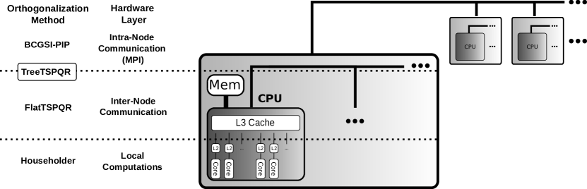
Figure 1: Design of the algorithm to the computer architecture. TreeTSPQR connects the FlatTSPQR algorithm for the computations on the nodes and the BCGS-PIP+ algorithm that is used for the reduction on the message passing level.

That means that TSPQR performs better for the solution of the problem on one node, while BCGS-PIP+ performs better for message passing environments. We therefore propose to combine the methods and use FlatTSPQR using HH for the local orthogonalization to solve the problem on one MPI rank and do the reduction of the results using the TreeTSPQR method, using the BCGS-PIP+ method for the reduction problem. This enables to utilize both advantages - good node performance and using the optimized inter-node communication pattern of the BCGS-PIP+ method. The design of the method and its adaption to the hardware is illustrated in Fig. 1.

6 Numerical Experiments

For the benchmarks and stability experiments we implemented the methods using the Eigen C++ framework [16]. We used MPI for the parallelization using one rank per core. The source code is provided as supplementary material.

6.1 Stability

To investigate the stability of the algorithms, we use the Stewart matrices presented in [22] to construct matrices with a given condition number. These matrices are constructed from a random matrix $A$, that is singular value decomposed $A=U\Sigma V^{T}$. The orthogonal matrices from the singular value decomposition are then recombined to the desired matrix $X=U\tilde{\Sigma}V^{T}$, where $\tilde{\Sigma}$ is a diagonal matrix with exponentially increasing diagonal entries $\frac{1}{\kappa},\ldots,1$, such that $X$ has the desired condition number $\kappa$. If not otherwise stated all experiments are carried out with $n=2^{16},{k=32}$ and $s=4$. For the TSPQR methods the problem is subdivided into problems of size $256$ rows.

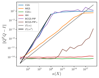
(a) basic variants

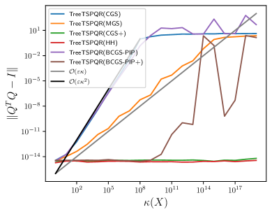
(b) TSPQR

Figure 2: Orthogonalization errors of presented algorithms for Stewart matrices with different condition numbers. Colors encode the different methods. The black and gray line mark $\mathcal{O}(\varepsilon\kappa)$ and $\mathcal{O}(\varepsilon\kappa^{2})$.

The first experiment is inspired by Carson et al. [5]. For that we compute the QR factorization of a Stewart matrix with different condition numbers using the presented algorithms applied on the $s$-block columns (Algorithm 2). Fig. 2a shows the orthogonalization error $\varepsilon_{\perp}$ as defined in equation (4) for the resulting $Q$-factor. We see that the traditional methods, Gram-Schmidt and Householder, behave as expected. The orthogonalization errors of the reiterated classical Gram-Schmidt method (CGS+) and the HH method are of order $\mathcal{O}(\varepsilon)$. For the modified Gram-Schmidt method the orthogonalization error is of order $\mathcal{O}(\kappa\varepsilon)$ and for the classical Gram-Schmidt method CGS it is of order $\mathcal{O}(\kappa^{2}\varepsilon)$.

The orthogonalization error of the BCGS-PIP method is of order $\mathcal{O}(\kappa^{2}\varepsilon)$, while its reiterated variant is stable up to a condition number satisfying

(40) $$\varepsilon\kappa^{2}\leq\frac{1}{2}.$$

The orthogonalization errors for different choices of subalgorithms algorithms in the TreeTSPQR algorithm are plotted in Fig. 2b. We see that the stability of the TreeTSPQR algorithm equals the stability of the used subalgorithm. The mentioned subalgorithm is used for the local as well as for the reduction step. The TreeTSPQR seems to be more sensible for condition (40) if BCGS+ is used as the subalgorithm.

In the next experiment we investigate how the orthogonalization error depends on the choice of the local and reduction subalgorithm respectively. For that we compute the QR factorization of a Stewart matrix with condition number $\kappa=${10}^{8}$$ with different combinations of subalgorithms. The result is shown in Fig. 3.

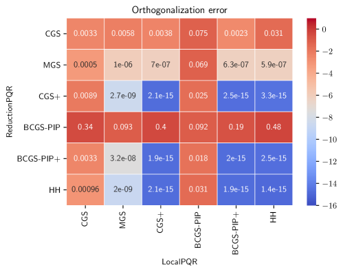
Figure 3: Orthogonalization errors for different combinations of local and reduction submethods used in TreeTSPQR for a Stewart matrix with condition number of $\kappa=${10}^{8}$$.

Red color indicates a high orthogonalization error, while blue color indicates stability. Columns encode the method that is used to solve the local problems and rows encode the reduction orthogonalization method. It shows that both subalgorithms must be stable to obtain a stable method.

Table 1: Stability results for the TreeTSPQR algorithm with different number of recursion levels and different number of local problems (local problem size).

	$e_{\perp}$			$\|A-QR\|$
level	BCGS-PIP	BCGS-PIP+	Householder	BCGS-PIP	BCGS-PIP+	Householder
0	$0.997\,49\text{\cdot}{10}^{-09}$	$2.328\,36\text{\cdot}{10}^{-15}$	$9.074\,92\text{\cdot}{10}^{-15}$	$5.8348\text{\cdot}{10}^{-16}$	$6.700\,02\text{\cdot}{10}^{-16}$	$4.076\,12\text{\cdot}{10}^{-15}$
1	$2.353\,87\text{\cdot}{10}^{-09}$	$2.391\,43\text{\cdot}{10}^{-15}$	$2.154\,42\text{\cdot}{10}^{-15}$	$5.549\,34\text{\cdot}{10}^{-16}$	$1.118\,75\text{\cdot}{10}^{-15}$	$1.197\,97\text{\cdot}{10}^{-15}$
2	$7.580\,58\text{\cdot}{10}^{-09}$	$3.600\,49\text{\cdot}{10}^{-15}$	$1.944\,08\text{\cdot}{10}^{-15}$	$7.169\,32\text{\cdot}{10}^{-16}$	$9.230\,65\text{\cdot}{10}^{-16}$	$1.2159\text{\cdot}{10}^{-15}$
3	$2.601\,33\text{\cdot}{10}^{-09}$	$4.386\,41\text{\cdot}{10}^{-15}$	$2.116\,58\text{\cdot}{10}^{-15}$	$1.067\,34\text{\cdot}{10}^{-15}$	$1.144\,09\text{\cdot}{10}^{-15}$	$1.457\,64\text{\cdot}{10}^{-15}$
4	$1.462\,54\text{\cdot}{10}^{-09}$	$3.1776\text{\cdot}{10}^{-15}$	$1.696\,69\text{\cdot}{10}^{-15}$	$9.238\,07\text{\cdot}{10}^{-16}$	$1.676\,34\text{\cdot}{10}^{-15}$	$1.475\,85\text{\cdot}{10}^{-15}$
5	$5.256\,72\text{\cdot}{10}^{-09}$	$4.021\,72\text{\cdot}{10}^{-15}$	$1.953\,51\text{\cdot}{10}^{-15}$	$1.377\,34\text{\cdot}{10}^{-15}$	$1.097\,62\text{\cdot}{10}^{-15}$	$1.574\,98\text{\cdot}{10}^{-15}$
6	$3.840\,84\text{\cdot}{10}^{-09}$	$4.359\,38\text{\cdot}{10}^{-15}$	$1.989\,05\text{\cdot}{10}^{-15}$	$1.234\,18\text{\cdot}{10}^{-15}$	$1.421\,75\text{\cdot}{10}^{-15}$	$1.828\,78\text{\cdot}{10}^{-15}$
7	$2.900\,05\text{\cdot}{10}^{-09}$	$5.2614\text{\cdot}{10}^{-15}$	$1.416\,94\text{\cdot}{10}^{-15}$	$1.4143\text{\cdot}{10}^{-15}$	$2.273\,28\text{\cdot}{10}^{-15}$	$1.958\,75\text{\cdot}{10}^{-15}$
8	$2.436\,57\text{\cdot}{10}^{-09}$	$5.300\,96\text{\cdot}{10}^{-15}$	$1.904\,36\text{\cdot}{10}^{-15}$	$1.943\,75\text{\cdot}{10}^{-15}$	$2.212\,07\text{\cdot}{10}^{-15}$	$2.382\,17\text{\cdot}{10}^{-15}$

(a) recursion levels

	$e_{\perp}$			$\|A-QR\|$
sub problems	BCGS-PIP	BCGS-PIP+	Householder	BCGS-PIP	BCGS-PIP+	Householder
8	$3.036\,84\text{\cdot}{10}^{-09}$	$1.768\,56\text{\cdot}{10}^{-15}$	$2.075\,94\text{\cdot}{10}^{-15}$	$6.498\,62\text{\cdot}{10}^{-16}$	$7.147\,92\text{\cdot}{10}^{-16}$	$9.896\,64\text{\cdot}{10}^{-16}$
16	$3.336\,63\text{\cdot}{10}^{-09}$	$2.583\,34\text{\cdot}{10}^{-15}$	$1.696\,39\text{\cdot}{10}^{-15}$	$8.597\,05\text{\cdot}{10}^{-16}$	$6.435\,50\text{\cdot}{10}^{-16}$	$8.273\,09\text{\cdot}{10}^{-16}$
32	$3.671\,68\text{\cdot}{10}^{-09}$	$2.630\,08\text{\cdot}{10}^{-15}$	$1.819\,35\text{\cdot}{10}^{-15}$	$6.066\,90\text{\cdot}{10}^{-16}$	$7.275\,82\text{\cdot}{10}^{-16}$	$8.169\,33\text{\cdot}{10}^{-16}$
64	$4.741\,07\text{\cdot}{10}^{-09}$	$2.256\,93\text{\cdot}{10}^{-15}$	$2.199\,55\text{\cdot}{10}^{-15}$	$6.117\,34\text{\cdot}{10}^{-16}$	$7.967\,82\text{\cdot}{10}^{-16}$	$1.427\,28\text{\cdot}{10}^{-15}$
128	$5.9833\text{\cdot}{10}^{-09}$	$3.619\,07\text{\cdot}{10}^{-15}$	$2.052\,85\text{\cdot}{10}^{-15}$	$7.718\,61\text{\cdot}{10}^{-16}$	$5.683\,21\text{\cdot}{10}^{-16}$	$9.568\,23\text{\cdot}{10}^{-16}$
256	$2.474\,85\text{\cdot}{10}^{-09}$	$2.600\,08\text{\cdot}{10}^{-15}$	$2.368\,96\text{\cdot}{10}^{-15}$	$5.627\,88\text{\cdot}{10}^{-16}$	$7.793\,41\text{\cdot}{10}^{-16}$	$1.219\,95\text{\cdot}{10}^{-15}$
512	$2.898\,39\text{\cdot}{10}^{-09}$	$2.463\,91\text{\cdot}{10}^{-15}$	$2.043\,22\text{\cdot}{10}^{-15}$	$6.684\,29\text{\cdot}{10}^{-16}$	$8.340\,59\text{\cdot}{10}^{-16}$	$1.324\,17\text{\cdot}{10}^{-15}$
1024	$5.327\,21\text{\cdot}{10}^{-09}$	$2.231\,19\text{\cdot}{10}^{-15}$	$2.421\,44\text{\cdot}{10}^{-15}$	$6.086\,44\text{\cdot}{10}^{-16}$	$4.983\,39\text{\cdot}{10}^{-16}$	$1.828\,94\text{\cdot}{10}^{-15}$

(b) number of subproblems

In a further experiment, we take a look at the errors dependent on the numbers of recursion levels in the TreeTSPQR algorithm and the number of processes used. Here we use a condition number of $\kappa=${10}^{4}$$. Table 1a shows the norm of the residual and the orthogonalization error of the TreeTSPQR algorithm with different number of recursion levels. Table 1b shows the residual norm and orthogonalization error of the TreeTSPQR method with differently many subproblems in two levels. The same system size was used, so if more subproblems are used the subproblems are of smaller size. We see that neither the orthogonality error nor the residual norm depend crucially on the number of used recursion levels or number of subproblems.

6.2 Performance

We demonstrate the performance advantages of the presented orthogonalization framework in this subsection. First, we consider the performance on a single node where message passing is cheap and the considerations in Section 5.1 are relevant. These experiments are carried out on our AMD Epic 7501 compute server with 64 physical cores. Each core has a $512\text{\,}\mathrm{kB}\text{/}$ L2 cache. The cores are organized on 8 sockets with 8 cores each, where all cores on a socket share an $8\text{\,}\mathrm{MB}\text{/}$ L3 cache.

To compare only the performance of the orthogonalization procedure, we compare the runtimes for computing a QR-factorization (Algorithm 2) instead of the Arnoldi method. With the Arnoldi method the timings would be unclear due to the application of the operator. We choose the problem size such that the L3 cache is exhausted. The input matrix for the QR-decomposition has $64$ columns (fix) and $2^{18}$ rows per process (weak scaling). This leads to a problem size of $64\cdot 2^{18}P\cdot 8$\mathrm{B}\text{/}$=P\cdot$128\text{\,}\mathrm{MB}\text{/}$$. We used a chunk size of $s=4$ and TSPQR methods use a local problem size of $n_{p}=2^{13}$ rows ($256\,$\mathrm{kB}\text{/}$$).

In a first benchmark we compare the runtimes of the different algorithms presented in this paper. Figure 4 shows the runtime of the different methods for a single process and for $64$ processes.

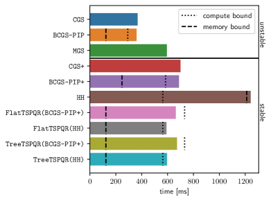
(a) Sequential

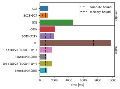
(b) Parallel ($64$ processes)

Figure 4: Comparison of algorithm runtimes on a single node with on one core (sequential) and on all 64 cores (parallel). Dashed and dotted lines mark the prediction of the roofline model. The solid black line separates unstable from stable methods.

At the top the unstable methods are displayed for comparison. Black vertical lines mark the compute- (dotted) and memory-bound (dashed) that is predicted by the roofline model in Section 5.1. To compute these bounds we measured the peak performance and memory bandwidth using the likwid-bench tool [24] and the stream_avx_fma benchmark. This benchmark is representative for the operations we perform in most algorithms. For one core we measured $\pi_{1}=$7.8\text{\,}\mathrm{Gflop}\text{/}\mathrm{s}$$ and $\beta_{1}=$18.4\text{\,}\mathrm{GB}\text{/}\mathrm{s}$$. For the parallel test case on all $64$ cores we measured $\pi_{64}=$364\text{\,}\mathrm{Gflop}\text{/}\mathrm{s}$$ and $\beta_{64}=$192\text{\,}\mathrm{GB}\text{/}\mathrm{s}$$.

The prediction of the performance model matches the result. The HH method is the slowest, due to the large amount of data that needs to be transferred from the memory. This issue is solved by the TSPQR methods which perform much better. In both cases the TSPQR methods are the fastest stable methods. In particular in the parallel case the TSPQR methods perform even faster as the BCGSI-PIP method, while preserving the stability of the used subalgorithm. TSPQR methods that use HH as subalgorithm are faster as the one used BCGS-PIP+. This is due to the higher computational effort of the BCGS-PIP+ method for the assembly of the output matrix $U$ if it used in TSPQR methods, as discussed in Section 5.1.

In the sequential case, the TSPQR methods using BCGS-PIP+ as a subalgorithm are even faster as predicted by the roofline model. This is due to the fact, that this algorithm uses a lot of matrix-matrix products which can be better optimized to achieve a higher flop-rate as the stream_avx_fma benchmark.

In the next benchmarks, we investigate the best local problem size for the TSPQR algorithms. Naturally, we want to choose the number of rows of the local spaces such that the local problem fits into the L2 cache. Unfortunately, the local problem size grows when the Krylov space grows, so that also the local problems grow.

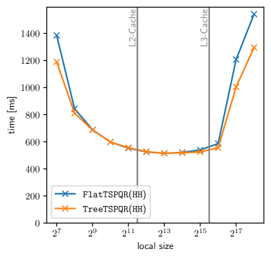
(a) Sequential

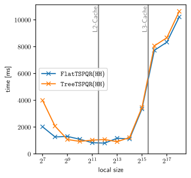
(b) Parallel ($64$ processes)

Figure 5: Benchmark for different local problem size in TSPQR algorithms. Using $s=2^{18}$ rows, $k=64$ and $s=8$ columns on each process (weak scaling). Gray vertical lines mark the size of the L2- and L3- cache.

In Fig. 5 the runtimes for computing the QR decomposition per number of local rows are shown for the same setting as in Fig. 4. The gray lines mark the size of the L2 and L3 cache for the largest case ($k=60,s=4$). We see that the minimum runtime is approximately at $2^{12}$ in the sequential and parallel case, which is slightly bigger than the L2 cache. For fewer local rows the method introduces overhead that leads to higher runtimes. For more local rows, the local problem becomes bigger than the cache which then leads to more communication between the memory and cache. We see also that the local characteristic of the algorithm has far more impact in the parallel setting. This is due to the fact that multiple cores share memory bandwidth, which leads to a smaller memory-bandwidth per process.

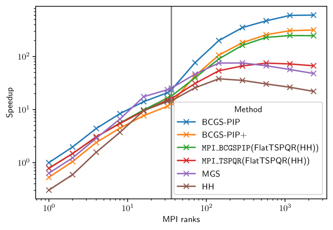
Figure 6: Strong-scaling benchmark on the PALMAII super computer on up to 2304 processes. The speedup is computed against the fastest method on one process (BCGS-PIP). Both axes are log-scale. Up to the gray vertical line the computation is on one node.

Finally, we validated the performance expectations for the message passing model from Section 5.2. For that we used the supercomputer PALMAII of the university of Münster. Fig. 6 shows the speedup for the same problem as used in the other benchmarks but in a strong scaling setting using up to 64 nodes with 36 processes each (2304 processes in total). The vertical gray line marks 36 processes, which is the limit for which the computation proceeds on one node. At the scaling limit the problem size is $n=\frac{2^{18}}{2304}\approx 114$ per process. We see that for large number of processes the performance of BMGS and HH stagnate, as they need many synchronization points, whereas the performance of the BCGS-PIP methods is much better. The runtime of the reiterated BCGS-PIP+ method is almost twice the runtime of the BCGS-PIP method. In our framework, we implemented two variants for the reduction of the TreeTSPQR method on the MPI level, BCGS-PIP+ and TSPQR, as discussed in Section 5.2. In Fig. 6 the labels are prefixed with MPI_ to indicate the respective usage on the MPI level. The MPI_TSPQR implementation performs not as good as the MPI_BCGS-PIP+ methods as it was predicted by out performance model. But we see that the performance of the MPI_TSPQR method is not decaying as fast as for the HH or MGS algorithms.

7 Conclusions and Outlook

In this paper we presented a new orthogonalization framework TSPQR that can be used to design orthogonalization algorithms for Krylov methods tailored on a specific hardware. The most common orthogonalization algorithms, Gram-Schmidt and Householder, are used as building blocks to solve smaller, local problems, that can be solved without communication. In principle other algorithms can be used as well. To demonstrate the usage and potential of the framework, we designed an algorithm for a CPU-based HPC-Cluster combining the Householder algorithm used for the local orthogonalization and the BCGS-PIP+ algorithm for reduction on the MPI layer. Furthermore, we presented a performance analysis for the designed method and presented numerical examples concerning the stability and performance.

The experiments showed that the novel framework can be used to design algorithms that perform as good as the performance-optimal BCGS-PIP algorithm, but preserve the stability of the used subalgorithm. In addition, it provides more flexibility for the developers and enables them to reuse existing implementations as building blocks.

The variety of orthogonalization algorithms that can be designed is manifold. A future goal would be to try out other orthogonalization methods as building blocks in this framework, e.g. paneled Householder algorithm [20] and see whether the performance could be further improved. Another goal would be to design algorithms for other hardware like GPUs and accelerators. Furthermore, we showed the stability of the TSPQR algorithms only experimentally. It would be worth to do an elaborate stability analysis to get further insights into the framework.

For the future, the MPI standard specification could be extended to allow stateful tree-reduction operations like it is needed by the TreeTSPQR algorithm. This would allow the vendor to optimize this operation on a specific hardware. In a further step, it could be beneficial to introduce network hardware, that implements the stateful tree-reduction where the state is stored on the network switches to improve this operation.

References

- [1] N. N. Abdelmalek, Round off error analysis for Gram-Schmidt method and solution of linear least squares problems, BIT Numerical Mathematics, 11 (1971), pp. 345–367, https://doi.org/10.1007/BF01939404.
- [2] J. L. Barlow and A. Smoktunowicz, Reorthogonalized block classical Gram-Schmidt, Numerische Mathematik, 123 (2013), pp. 395–423, https://doi.org/10.1007/s00211-012-0496-2.
- [3] D. Bielich, J. Langou, S. Thomas, K. Swirydowicz, I. Yamazaki, and E. G. Boman, Low-synch Gram-Schmidt with delayed reorthogonalization for Krylov solvers, (2021), https://arxiv.org/abs/2104.01253.
- [4] E. Carson, K. Lund, and M. Rozložník, The stability of block variants of classical Gram–Schmidt, SIAM Journal on Matrix Analysis and Applications, 42 (2021), pp. 1365–1380, https://doi.org/10.1137/21M1394424.
- [5] E. Carson, K. Lund, M. Rozložník, and S. Thomas, Block Gram-Schmidt algorithms and their stability properties, Linear Algebra and its Applications, 638 (2022), pp. 150–195, https://doi.org/10.1016/j.laa.2021.12.017.
- [6] D. Culler, R. Karp, D. Patterson, A. Sahay, K. E. Schauser, E. Santos, R. Subramonian, and T. Von Eicken, Logp: Towards a realistic model of parallel computation, in Proceedings of the fourth ACM SIGPLAN symposium on Principles and practice of parallel programming, 1993, pp. 1–12, https://doi.org/10.1145/155332.155333.
- [7] J. Demmel, L. Grigori, M. Hoemmen, and J. Langou, Communication-optimal parallel and sequential QR and LU factorizations: theory and practice, 2008, https://arxiv.org/abs/0806.2159.
- [8] J. Demmel, L. Grigori, M. Hoemmen, and J. Langou, Communication-optimal parallel and sequential QR and LU factorizations, SIAM Journal on Scientific Computing, 34 (2012), pp. A206–A239, https://doi.org/10.1137/080731992.
- [9] J. Dongarra, P. Beckman, T. Moore, P. Aerts, G. Aloisio, J.-C. Andre, D. Barkai, J.-Y. Berthou, T. Boku, B. Braunschweig, et al., The international exascale software project roadmap, The international journal of high performance computing applications, 25 (2011), pp. 3–60, https://doi.org/10.1177/1094342010391989.
- [10] N.-A. Dreier, Hardware-oriented Krylov methods for high-performance computing, PhD thesis, 2020, https://miami.uni-muenster.de/Record/4828cbac-b0f1-4355-a08e-af984cd30c4a. supervision: C. Engwer.
- [11] N.-A. Dreier and C. Engwer, Strategies for the vectorized block conjugate gradients method, in Numerical Mathematics and Advanced Applications-ENUMATH 2019, vol. 139, Springer, 2020, https://doi.org/10.1007/978-3-030-55874-1_37.
- [12] P. Ghysels, T. J. Ashby, K. Meerbergen, and W. Vanroose, Hiding global communication latency in the GMRES algorithm on massively parallel machines, SIAM Journal on Scientific Computing, 35 (2013), pp. C48–C71, https://doi.org/10.1137/12086563X.
- [13] L. Giraud, J. Langou, M. Rozložník, and J. van den Eshof, Rounding error analysis of the classical Gram-Schmidt orthogonalization process, Numerische Mathematik, 101 (2005), pp. 87–100, https://doi.org/10.1007/s00211-005-0615-4.
- [14] G. H. Golub and R. Underwood, The block Lanczos method for computing eigenvalues, in Mathematical software, Elsevier, 1977, pp. 361–377, https://doi.org/10.1016/B978-0-12-587260-7.50018-2.
- [15] G. H. Golub and C. Van Loan, Matrix computations, JHU press, 2013.
- [16] G. Guennebaud, B. Jacob, et al., Eigen v3.4, 2010, http://eigen.tuxfamily.org.
- [17] W. Jalby and B. Philippe, Stability analysis and improvement of the block Gram-Schmidt algorithm, SIAM journal on scientific and statistical computing, 12 (1991), pp. 1058–1073, https://doi.org/10.1137/0912056.
- [18] D. P. O’Leary, The block conjugate gradient algorithm and related methods, Linear algebra and its applications, 29 (1980), pp. 293–322, https://doi.org/10.1016/0024-3795(80)90247-5.
- [19] M. Sadkane, Block-Arnoldi and Davidson methods for unsymmetric large eigenvalue problems, Numerische Mathematik, 64 (1993), pp. 195–211, https://doi.org/10.1007/BF01388687.
- [20] R. Schreiber and C. Van Loan, A storage-efficient wy representation for products of Householder transformations, SIAM Journal on Scientific and Statistical Computing, 10 (1989), pp. 53–57, https://doi.org/10.1137/0910005.
- [21] V. Simoncini and E. Gallopoulos, Convergence properties of block GMRES and matrix polynomials, Linear Algebra and its Applications, 247 (1996), pp. 97–119, https://doi.org/10.1016/0024-3795(95)00093-3.
- [22] G. W. Stewart, Block Gram–Schmidt orthogonalization, SIAM Journal on Scientific Computing, 31 (2008), pp. 761–775, https://doi.org/10.1137/070682563.
- [23] K. Swirydowicz, J. Langou, S. Ananthan, U. Yang, and S. Thomas, Low synchronization Gram–Schmidt and generalized minimal residual algorithms, Numerical Linear Algebra with Applications, 28 (2021), p. e2343, https://doi.org/10.1002/nla.2343.
- [24] J. Treibig, G. Hager, and G. Wellein, Likwid: Lightweight performance tools, in Competence in High Performance Computing 2010, C. Bischof, H.-G. Hegering, W. E. Nagel, and G. Wittum, eds., Berlin, Heidelberg, 2012, Springer Berlin Heidelberg, pp. 165–175, https://doi.org/10.1007/978-3-642-24025-6_14.
- [25] H. F. Walker, Implementation of the GMRES method using Householder transformations, SIAM Journal on Scientific and Statistical Computing, 9 (1988), pp. 152–163, https://doi.org/10.1137/0909010.
- [26] S. Williams, A. Waterman, and D. Patterson, Roofline: An insightful visual performance model for multicore architectures, Commun. ACM, 52 (2009), p. 65–76, https://doi.org/10.1145/1498765.1498785.
- [27] Y. Yamamoto, Y. Nakatsukasa, Y. Yanagisawa, and T. Fukaya, Roundoff error analysis of the CholeskyQR2 algorithm in an oblique inner product, JSIAM Letters, 8 (2016), pp. 5–8, https://doi.org/10.14495/jsiaml.8.5.
- [28] I. Yamazaki, S. Thomas, M. Hoemmen, E. G. Boman, K. Świrydowicz, and J. J. Elliott, Low-synchronization orthogonalization schemes for s-step and pipelined Krylov solvers in Trilinos, in Proceedings of the 2020 SIAM Conference on Parallel Processing for Scientific Computing (PP), pp. 118–128, https://doi.org/10.1137/1.9781611976137.11.