Structural and thermodynamic properties of fluids whose molecules interact via one-, two-, and three-step potentials

Abstract

The structural and thermodynamic properties of fluids whose molecules interact via potentials with a hard-core plus a square well, a square shoulder, and a second square well, are considered. Those properties are derived by using a (semi-analytical) rational-function approximation method as a particular case of the more general formulation provided earlier involving potentials with a hard-core plus $n$ piecewise constant sections. Comparison of the results with recent simulation data confirms the usefulness of the approach.

1 Introduction

Undoubtedly, the late Douglas Henderson was a recognized international leader in the theory of liquids. In this area he provided significant contributions, such as the one with John Barker concerning the perturbation theory of fluids. In particular, in their outstanding paper What is “liquid”? Understanding the states of matter, published in Reviews of Modern Physics [1], Barker and Henderson clearly laid out the ground for further developments in liquid-state theory. There they wrote “The aim of the physics of liquids is to understand why particular phases are stable in particular ranges of temperature and density (phase diagrams; …), and to relate the stability, structure, and dynamical properties of fluid phases to the size and shape of molecules, atoms, or ions and the nature of the forces between them (which in turn are determined by the electronic properties).” In this regard, the discrete potentials including the square-well (SW), the triangle-well, or the square-shoulder (SS) potentials, as well as potentials with a hard-core plus piecewise constant regions, have been important in advancing in this direction as simple models of intermolecular interaction. Using such potentials, problems such as liquid-liquid transitions [2, 3, 4, 5], colloidal interactions [6], the anomalous density behavior of water and supercooled fluids [7, 8], and the thermodynamic and transport properties of Lennard-Jones fluids [9, 10], among others, have been successfully addressed.

Very recently Perdomo-Pérez et al. [11] have considered fluids with competing interactions modeled through a succession of SW and SS potentials. Their main goal was to systematically study the effect of each potential contribution on the physical properties of a competing interaction fluid. Since the discrete potentials are discontinuous and they cannot be directly used in simulation methods that require the explicit calculation of the force at the breakpoints, they further determined suitable continuous and differentiable potentials that, apart from mimicking some of the properties of their discrete potential counterparts, had the same reduced second virial coefficient. With this approach, they have produced new simulation data on both the radial distribution function (RDF) and the compressibility factor of fluids interacting via those discrete-like potentials, thus extending and complementing the (relatively scarce) earlier simulation data [6, 12, 13, 14] on these properties.

In previous work [15], we used the rational-function approximation (RFA) methodology [16], which is a semi-analytical approach, to derive the general formulae for the structural properties of fluids whose molecules interact via discrete potentials with a hard core plus an arbitrary number of piecewise constant sections of different widths and heights, and compared the outcome with the then available computer simulation results [14]. This work led later to the consideration of the special case in which the fluids were constituted by molecules whose interaction potential consisted of a discrete potential with a hard core plus different combinations of a repulsive shoulder and an attractive well [17]. The question then naturally arises as to whether our theoretical development will also perform well when compared to the new simulation data involving fluids interacting via a potential with a hard-core plus a SW, a SS, and a second SW. The aim of this paper is precisely to evaluate such performance.

The paper is organized as follows. In order to make it self-contained, in Section 2 we provide the background material of the RFA approach for discrete fluids whose intermolecular potential has a hard-core plus $n$ piecewise constant sections. This is followed by Section 3, which contains the results of our calculations for illustrative cases and their comparison with the recent simulation data for such cases [11]. We close the paper in Section 4 with further discussion and some concluding remarks.

2 The rational-function approximation

In this section we provide a brief but self-contained account of the RFA methodology as applied to our fluid whose molecules interact through a potential with a hard-core plus $n$ piecewise constant regions. For a more detailed account, we refer the reader to Refs. [15, 16].

2.1 Formal expressions

Let us recall first some general relations between the thermodynamic and structural properties of fluids. The virial route to the equation of state leads to [1, 18, 16]

$$Z\equiv\frac{p}{\rho k_{B}T}= 1-\frac{\rho}{6k_{B}T}\int d\mathbf{r}\,g(r)r\frac{\partial\phi(r)}{\partial r}$$

$$= 1+\frac{\rho}{6}\int d\mathbf{r}\,y(r)r\frac{\partial e^{-\phi(r)/k_{B}T}}{\partial r},$$ (1)

where $Z$ is the compressibility factor, $p$ is the pressure, $\rho$ is the number density, $k_{B}$ is the Boltzmann constant, $T$ is the absolute temperature, $\phi(r)$ is the interaction potential (assumed to be spherically symmetric and pairwise additive), $g(r)$ is the RDF, which is a measure of the probability of finding a molecule at a distance $r$ from another molecule, and $y(r)\equiv g(r)e^{\phi(r)/k_{B}T}$ is the so-called cavity function. On the other hand, the static structure factor $S(q)$, which is related to the Fourier transform of $g(r)-1$ by

$$S(q)=1+\rho\int d\mathbf{r}\,e^{-\imath\mathbf{q}\cdot\mathbf{r}}[g(r)-1],$$ (2)

where $\imath$ is the imaginary unit and $q$ is the wavenumber, also provides another connection between the structural and thermodynamic properties. In fact, the isothermal compressibility of the fluid, $\kappa_{T}=\rho^{-1}\left(\partial\rho/\partial p\right)_{T}$ is directly related to the long-wavelength limit of the structure factor, namely

$$\chi_{T}\equiv\rho k_{\textrm{B}}T\kappa_{T}=S(0),$$ (3)

where $\chi_{T}$ is the isothermal susceptibility. This leads to the compressibility route to the equation of state:

$$Z=\int_{0}^{1}\frac{dt}{\chi_{T}(\rho t)}.$$ (4)

It is also convenient at this stage to introduce the Laplace transform $G(s)$ of $rg(r)$, i.e.,

$$G(s)=\int_{0}^{\infty}dr\,e^{-rs}rg(r).$$ (5)

In terms of $G(s)$, the static structure factor is simply expressed as

$$S(q)=1-2\pi\rho\left.\frac{G(s)-G(-s)}{s}\right|_{s=\imath q}.$$ (6)

Let us now consider the piecewise constant potential of our fluid given by

$$\phi(r)=\left\{\begin{array}[]{ll}\infty,&r<\sigma,\\ \epsilon_{1},&\sigma<r<\lambda_{1},\\ \epsilon_{2},&\lambda_{1}<r<\lambda_{2},\\ \vdots&\vdots\\ \epsilon_{n},&\lambda_{n-1}<r<\lambda_{n},\\ 0,&r>\lambda_{n}.\end{array}\right.$$ (7)

This potential is characterized by a hard core of diameter $\sigma$ and $n$ steps of heights $\epsilon_{j}$ and widths $\lambda_{j}-\lambda_{j-1}$, where henceforth the conventions $\lambda_{0}=1$, $\epsilon_{0}=\infty$, and $\epsilon_{n+1}=0$ are understood. Without loss of generality in what follows we will take the hard-core diameter $\sigma=1$ as the length unit and $|\epsilon_{1}|$ as the energy unit.

For the potential (7), the virial route (2.1) to the equation of state adopts the specially appealing form

$$Z=1+4\eta\sum_{j=0}^{n}\lambda_{j}^{3}\Delta g(\lambda_{j}),$$ (8)

where $\eta\equiv\frac{\pi}{6}\rho^{*}$ is the packing fraction ($\rho^{*}=\rho\sigma^{3}$ being the reduced density), $\Delta g(\lambda_{j})\equiv g(\lambda_{j}^{+})-g(\lambda_{j}^{-})$ is the jump of the RDF at $r=\lambda_{j}$, and use has been made of the continuity of $y(r)$.

We focus now on some exact mathematical properties of the function $G(s)$. More specifically, we introduce an auxiliary function $F(s)$ defined through

$$G(s)=s\frac{F(s)e^{-s}}{1+12\eta F(s)e^{-s}},$$ (9)

so that Laplace inversion of Eq. (9) provides a useful representation of the RDF:

$$g(r)=r^{-1}\sum_{m=1}^{\infty}(-12\eta)^{m-1}f_{m}(r-m)\Theta(r-m),$$ (10)

where $f_{m}(r)=\mathcal{L}^{-1}\left[s[F(s)]^{m}\right]$ is the inverse Laplace transform of $s[F(s)]^{m}$ and $\Theta(r)$ is the Heaviside step function. The exact behaviors for large $s$ and small $s$ of the auxiliary function $F(s)$ are [19, 20, 21, 15, 16, 22]

$$F(s)\sim s^{-2},\quad s\rightarrow\infty,$$ (11a)

$$F(s)= -\frac{1}{12\eta}\left(1+s+\frac{1}{2}s^{2}+\frac{1+2\eta}{12\eta}s^{3}+\frac{2+\eta}{24\eta}s^{4}\right)$$

$$+F_{5}s^{5}+F_{6}s^{6}+{\cal O}(s^{7}),$$ (11b)

where the values of the coefficients $F_{5}$ and $F_{6}$ determine the value of $S(0)$, and hence of the isothermal compressibility, by

$$S(0)=3456\eta^{3}\left(F_{5}-F_{6}\right)-1+8\eta+2\eta^{2}.$$ (12)

Let us now decompose $F(s)$ as

$$F(s)=\sum_{j=0}^{n}R_{j}(s)e^{-(\lambda_{j}-1)s}.$$ (13)

This decomposition reflects the discontinuities of $g(r)$ at the points $r=\lambda_{j}$. More specifically,

$$\Delta g(\lambda_{j})=\frac{1}{\lambda_{j}}\lim_{s\to\infty}s^{2}R_{j}(s)=\frac{1}{\lambda_{j}}\xi_{j}(0),\quad j=0,1,\ldots,n,$$ (14)

where $\xi_{j}(r)=\mathcal{L}^{-1}\left[sR_{j}(s)\right]$. Thus,

$$f_{1}(r)=\sum_{j=0}^{n}\xi_{j}(r-\lambda_{j}+1)\Theta(r-\lambda_{j}+1).$$ (15)

2.2 Our approximation

2.2.1 RDF

Now we assume the following rational-function approximation for $R_{j}(s)$:

$$R_{j}(s)=-\frac{1}{12\eta}\frac{A_{j}+B_{j}s}{1+S_{1}s+S_{2}s^{2}+S_{3}s^{3}},\quad j=0,1,\ldots,n.$$ (16)

Since the degree difference between the numerator and denominator of $R_{0}(s)$ is equal to $2$, the form (16) ensures the consistency with Eq. (11a). Moreover, according to Eq. (14),

$$\Delta g(\lambda_{j})=-\frac{1}{12\eta\lambda_{j}}\frac{B_{j}}{S_{3}},\quad j=0,1,\ldots,n.$$ (17)

For simplicity, the parameters $\{A_{j},j=0,1,\ldots,n\}$ are assumed to be independent of density, yielding [15]

$$A_{j}=e^{-\epsilon_{j+1}/k_{B}T}-e^{-\epsilon_{j}/k_{B}T}.$$ (18)

Next, the exact expansion (11) gives

$$S_{1}=\Omega_{0}-\Lambda_{1},$$ (19a)

$$S_{2}=\frac{1}{2}\Lambda_{2}-\Omega_{1},$$ (19b)

$$S_{3}=\frac{1}{2}\Omega_{2}-\frac{1}{6}\Lambda_{3}-\frac{1}{12\eta},$$ (19c)

$$\Lambda_{1}+\frac{1}{2}\eta\Lambda_{4}=\Omega_{0}+2\eta\Omega_{3},$$ (19d)

where

$$\Lambda_{\ell}\equiv\sum_{j=0}^{n}A_{j}\lambda_{j}^{\ell},\quad\Omega_{\ell}\equiv\sum_{j=0}^{n}B_{j}\lambda_{j}^{\ell}.$$ (20)

Equations (19a)–(19c) give $S_{1}$, $S_{2}$, and $S_{3}$ as linear combinations of the coefficients $\{B_{j}\}$, while the constraint (19d) allows us to express one of the latter coefficients, say $B_{0}$, in terms of the other ones. To close the problem, we then need $n$ additional constraints to determine $\{B_{j}\}$. The continuity of the cavity function imposes the conditions

$$\xi_{j}(0)=e^{\epsilon_{j}/k_{B}T}A_{j}\sum_{i=0}^{j-1}\xi_{i}(\lambda_{j}-\lambda_{i}),\quad j=1,\ldots,n.$$ (21)

Application of the residue theorem gives

$$\xi_{j}(r)=-\frac{1}{12\eta}\sum_{\alpha=1}^{3}\frac{A_{j}+B_{j}s_{\alpha}}{S_{1}+2S_{2}s_{\alpha}+3S_{3}s_{\alpha}^{2}}s_{\alpha}e^{s_{\alpha}r},$$ (22)

where $s_{\alpha}$ ($\alpha=1,2,3$) are the three roots of the cubic equation $1+S_{1}s_{\alpha}+S_{2}s_{\alpha}^{2}+S_{3}s_{\alpha}^{3}=0$. Thus, taking into account Eqs. (14) and (17), Eq. (21) becomes

$$\frac{B_{j}}{S_{3}}= e^{\epsilon_{j}/k_{B}T}A_{j}\sum_{\alpha=1}^{3}\frac{s_{\alpha}e^{\lambda_{j}s_{\alpha}}}{S_{1}+2S_{2}s_{\alpha}+3S_{3}s_{\alpha}^{2}}$$

$$\times\sum_{i=0}^{j-1}(A_{i}+B_{i}s_{\alpha})e^{-\lambda_{i}s_{\alpha}},\quad j=1,\ldots,n.$$ (23)

Equation (23), complemented by Eqs. (19), must be solved numerically. Once $F(s)$ is fully determined, Eq. (10) provides the RDF, where $f_{m}(r)$ can be obtained from the residue theorem or, alternatively, by numerical Laplace inversion [23].

It can be proved [20, 15, 16] that the RFA reduces to the exact solutions of the Percus–Yevick integral equation theory for hard spheres and sticky hard spheres in the appropriate limits.

2.2.2 Equation of state

In the RFA, the equation of state from the virial route is obtained by inserting Eq. (17) into Eq. (8):

$$Z=1-\frac{{\Omega}_{2}}{3S_{3}}.$$ (24)

In the case of the compressibility route, we need to expand $F(s)$ in powers of $s$, identify the coefficients $F_{5}$ and $F_{6}$, and make use of Eqs. (3) and (12). After some algebra, one finds

$$\chi_{T}= 1+4\eta\left(\Lambda_{3}-3\Lambda_{1}\Lambda_{2}+3\Lambda_{2}{\Omega}_{0}+6\Lambda_{1}{\Omega}_{1}-6{\Omega}_{0}{\Omega}_{1}\right.$$

$$\left.-3{\Omega}_{2}\right)+\frac{2}{5}\eta^{2}\left(\Lambda_{6}-6\Lambda_{1}\Lambda_{5}+6\Lambda_{5}{\Omega}_{0}+30\Lambda_{1}{\Omega}_{4}\right.$$

$$\left.-30{\Omega}_{0}{\Omega}_{4}-6{\Omega}_{5}\right).$$ (25)

The corresponding compressibility factor is obtained from Eq. (4) by numerical integration.

2.3 RDF to first order in density and third virial coefficient

For the sake of completeness, let us obtain the explicit expressions of the RFA in the low-density regime.

2.3.1 RDF to first order in density

In the low-density limit we can write

$$B_{j}=A_{j}\left(\lambda_{j}+\eta X_{j}\right)+\mathcal{O}(\eta^{2}),\quad j=0,1,\ldots,n,$$ (26)

where the first-order coefficients $X_{j}$ are to be determined. From Eqs. (19),

$$A_{0}X_{0}=-\sum_{i=1}^{n}A_{i}X_{i}-\frac{3}{2}\Lambda_{4},$$ (27a)

$$S_{1}=-\frac{3}{2}\eta\Lambda_{4}+\mathcal{O}(\eta^{2}),$$ (27b)

$$S_{2}=-\frac{1}{2}\Lambda_{2}-\eta\sum_{j=0}^{n}A_{j}X_{j}\lambda_{j}+\mathcal{O}(\eta^{2}),$$ (27c)

$$S_{3}=-\frac{1}{12\eta}+\frac{1}{3}\Lambda_{3}+\frac{\eta}{2}\sum_{j=0}^{n}A_{j}X_{j}\lambda_{j}^{2}+\mathcal{O}(\eta^{2}).$$ (27d)

Therefore, Eq. (16) becomes

$$R_{j}(s)=R_{j}^{(0)}(s)+\eta R_{j}^{(1)}(s)+\mathcal{O}(\eta^{2}),$$ (28)

where

$$\frac{R_{j}^{(0)}(s)}{A_{j}}=s^{-3}+\lambda_{j}s^{-2},$$ (29a)

$$\frac{R_{j}^{(1)}(s)}{A_{j}}=X_{j}s^{-2}+12(s^{-1}+\lambda_{j})\left(s^{-5}-\frac{s^{-3}\Lambda_{2}}{2}+\frac{s^{-2}\Lambda_{3}}{3}\right).$$ (29b)

This yields

$$\xi_{j}(r)\equiv\mathcal{L}^{-1}\left[sR_{j}(s)\right]=\xi_{j}^{(0)}(r)+\eta\xi_{j}^{(1)}(r)+\mathcal{O}(\eta^{2}),$$ (30)

with

$$\frac{\xi_{j}^{(0)}(r)}{A_{j}}=\lambda_{j}+r,$$ (31a)

$$\frac{\xi_{j}^{(1)}(r)}{A_{j}}=X_{j}+\frac{r^{3}}{2}(4\lambda_{j}+r)-3\Lambda_{2}r(2\lambda_{j}+r)+4\Lambda_{3}(\lambda_{j}+r).$$ (31b)

We still need to determine the coefficients $\{X_{j},j=1,\ldots,n\}$. From the continuity conditions (21), we get

$$X_{j}=e^{\epsilon_{j}/k_{B}T}\left(\sum_{i=0}^{j-1}A_{i}X_{i}+K_{j}\right),\quad j=1,\ldots,n,$$ (32)

where

$$K_{j}\equiv\sum_{i=0}^{j-1}A_{i}\left[\frac{(\lambda_{j}-\lambda_{i})^{3}}{2}(\lambda_{j}+3\lambda_{i})-3\Lambda_{2}(\lambda_{j}^{2}-\lambda_{i}^{2})\right].$$ (33)

It can be checked that the solution to Eq. (32) is

$$X_{j}=\sum_{i=j+1}^{n}A_{i}^{+}K_{i}+e^{\epsilon_{j+1}/k_{B}T}K_{j}-\frac{3}{2}\Lambda_{4},\quad 1\leq j\leq n,$$ (34)

where

$$A_{j}^{+}\equiv e^{\epsilon_{j+1}/k_{B}T}-e^{\epsilon_{j}/k_{B}T},\quad j=0,1,\ldots,n.$$ (35)

Taking $K_{0}=0$, Eq. (34) can still be used to get $X_{0}$, thus obtaining an expression equivalent to Eq. (27a).

Once we have obtained all the RFA parameters to first order in density, let us evaluate the RDF to that order. Recalling Eqs. (9) and (13), we get

$$G(s)=G^{(0)}(s)+\eta G^{(1)}(s)+\mathcal{O}(\eta^{2}),$$ (36)

where

$$G^{(0)}(s)=sF^{(0)}(s)e^{-s},$$ (37a)

$$G^{(1)}(s)=sF^{(1)}(s)e^{-s}-12s\left[F^{(0)}(s)\right]^{2}e^{-2s},$$ (37b)

with

$$F^{(0)}(s)\equiv\sum_{j=0}^{n}R_{j}^{(0)}(s)e^{-(\lambda_{j}-1)s},$$ (38a)

$$F^{(1)}(s)\equiv\sum_{j=0}^{n}R_{j}^{(1)}(s)e^{-(\lambda_{j}-1)s}.$$ (38b)

Thus,

$$g(r)=g^{(0)}(r)+\eta g^{(1)}(r)+\mathcal{O}(\eta^{2}),$$ (39)

where

$$g^{(0)}(r)= r^{-1}\sum_{j=0}^{n}\xi^{(0)}(r-\lambda_{j})\Theta(r-\lambda_{j})$$

$$= \sum_{j=0}^{n}A_{j}\Theta(r-\lambda_{j}),$$ (40a)

$$g^{(1)}(r)= r^{-1}\sum_{j=0}^{n}\xi^{(1)}(r-\lambda_{j})\Theta(r-\lambda_{j})$$

$$-12\eta r^{-1}f_{2}^{(0)}(r-2)\Theta(r-2),$$ (40b)

$f_{2}^{(0)}(r)$ being the inverse Laplace transform of $s\left[F^{(0)}(s)\right]^{2}$. Using

$$s\left[F^{(0)}(s)\right]^{2}= \sum_{i=0}^{n}\sum_{j=0}^{n}A_{i}A_{j}\left[s^{-5}+(\lambda_{i}+\lambda_{j})s^{-4}\right.$$

$$\left.+\lambda_{i}\lambda_{j}s^{-3}\right]e^{-(\lambda_{i}+\lambda_{j}-2)s},$$ (41)

we get

$$f_{2}^{(0)}(r-2)= \sum_{i=0}^{n}\sum_{j=0}^{n}A_{i}A_{j}\frac{(r-\lambda_{i}-\lambda_{j})^{2}}{24}\left[(r-\lambda_{i}-\lambda_{j})^{2}\right.$$

$$\left.+4(\lambda_{i}+\lambda_{j})(r-\lambda_{i}-\lambda_{j})+12\lambda_{i}\lambda_{j}\right]$$

$$\times\Theta(r-\lambda_{i}-\lambda_{j}).$$ (42)

It can be checked that

$$g^{(0)}(r)=1,\quad r\geq\lambda_{n},$$ (43a)

$$g^{(1)}(r)=0,\quad r\geq 2\lambda_{n}.$$ (43b)

Equations (39), (40), and (2.3.1) provide the RDF to first order in density within the RFA. While $g^{(0)}(r)$ is exact, $g^{(1)}(r)$ is approximate. From standard statistical-mechanical tools [16, 18], the exact result can be written as

$$g^{(1)}_{\text{exact}}(r)=e^{-\phi(r)/k_{B}T}y^{(1)}_{\text{exact}}(r),$$ (44a)

$$y^{(1)}_{\text{exact}}(r)=\frac{3}{\pi^{3}}\int_{0}^{\infty}dq\,q^{2}\frac{\sin(qr)}{qr}\left[\widetilde{f}(q)\right]^{2},$$ (44b)

where

$$\widetilde{f}(q)= 4\pi\int_{0}^{\infty}dr\,r^{2}\frac{\sin(qr)}{qr}\left[e^{-\phi(r)/k_{B}T}-1\right]$$

$$= 4\pi\sum_{j=0}^{n}A_{j}\frac{q\lambda_{j}\cos(q\lambda_{j})-\sin(q\lambda_{j})}{q^{3}}$$ (45)

is the Fourier transform of the Mayer function. The $q$-integration can be performed to get

$$y^{(1)}_{\text{exact}}(r\geq 1)= \frac{1}{2}\sum_{i=0}^{n}\sum_{j=0}^{n}A_{i}A_{j}\frac{(\lambda_{i}+\lambda_{j}-r)^{2}}{r}$$

$$\times[(r+\lambda_{i}+\lambda_{j})^{2}-4(\lambda_{i}^{2}+\lambda_{j}^{2}-\lambda_{i}\lambda_{j})]$$

$$\times\Theta(\lambda_{i}+\lambda_{j}-r).$$ (46)

Note that, since $\lambda_{j}>1$, one always has $\lambda_{i}+\lambda_{j}>r$ if $r\leq 2$, so that the term $\Theta(\lambda_{i}+\lambda_{j}-r)$ is not needed in that case. It can be checked that the RDF function $g^{(1)}(r)$ differs from $g^{(1)}_{\text{exact}}(r)$ in the interval $1\leq r\leq\lambda_{n}\leq 2$ only.

Table 1: Systems examined in this paper.

		SW parameters			SS parameters			SW parameters
Label	$n$	$\lambda_{1}$	$\epsilon_{1}$		$\lambda_{2}$	$\epsilon_{2}$		$\lambda_{3}$	$\epsilon_{3}$	Graph
A	$1$	$1.15$	$-1$
B1	$2$	$1.15$	$-1$		$1.25$	$0.25$
B2	$2$	$1.15$	$-1$		$1.25$	$1.00$
B3	$2$	$1.15$	$-1$		$1.50$	$0.25$
B4	$2$	$1.15$	$-1$		$1.50$	$1.00$
C1	$3$	$1.15$	$-1$		$1.50$	$0.50$		$2$	$-0.1$
C2	$3$	$1.15$	$-1$		$1.50$	$0.50$		$2$	$-0.2$

2.3.2 Second and third virial coefficients

According to the virial route, Eq. (8),

$$Z= 1+4\eta\sum_{j=0}^{n}\lambda_{j}^{2}\xi_{j}(0)$$

$$= 1+b_{2}\eta+b_{3,v}\eta^{2}+\mathcal{O}(\eta^{3}).$$ (47)

From Eqs. (30) and (31) or, equivalently, from Eq. (24), we can identify

$$b_{2}=4\Lambda_{3},$$ (48)

$$b_{3,v}=16\Lambda_{3}^{2}+4\sum_{j=0}^{n}A_{j}X_{j}\lambda_{j}^{2}.$$ (49)

Now we consider the compressibility route, Eqs. (3) and (4),

$$\chi_{T}= 1+24\eta\int_{0}^{\infty}dr\,r^{2}\left[g(r)-1\right]$$

$$= 1-2b_{2}\eta+(4b_{2}^{2}-3b_{3,c})\eta^{2}+\mathcal{O}(\eta^{3}),$$ (50)

where

$$b_{3,c}=\frac{64}{3}\Lambda_{3}^{2}-8\int_{0}^{2\lambda_{n}}dr\,r^{2}g^{(1)}(r).$$ (51)

An equivalent, but more explicit, closed expression for $b_{3,c}$ is obtained from Eq. (2.2.2):

$$b_{3,c}=\frac{64}{3}\Lambda_{3}^{2}-6\Lambda_{2}\Lambda_{4}+\frac{2}{3}\Lambda_{6}+4\sum_{j=0}^{n}A_{j}X_{j}\lambda_{j}^{2}.$$ (52)

The difference between $b_{3,c}$ and $b_{3,v}$ is

$$b_{3,c}-b_{3,v}=\frac{2}{3}\left(8\Lambda_{3}^{2}+\Lambda_{6}-9\Lambda_{2}\Lambda_{4}\right).$$ (53)

This lack of thermodynamic consistency between the virial and compressibility routes is an expected consequence of the approximate character of the RFA.

Taking into account the property $\Delta g(\lambda_{j})=A_{j}y(\lambda_{j})$, the exact result is

$$b_{3,\text{exact}}=4\sum_{j=0}^{n}\lambda_{j}^{3}A_{j}y^{(1)}_{\text{exact}}(\lambda_{j}),$$ (54)

where $y^{(1)}_{\text{exact}}(r)$ is given by Eq. (2.3.1).

3 Illustrative results

In this section we illustrate the results of our approach by examining their performance against recent simulation data [11] for both the structural and thermodynamic properties of this kind of fluids. For this purpose, it is convenient to order the different systems according to the number of steps after the hard core, so that the label A will indicate a single SW, the label B a SW followed by a SS, and the label C a SW followed by a SS and a second SW. According to the above nomenclature, Table 1 includes the values of the parameters $\{\lambda_{j},\epsilon_{j}\}$ for each one of the seven examined systems.

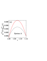
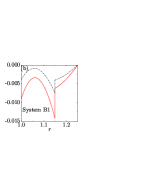
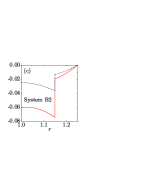
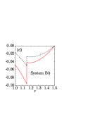
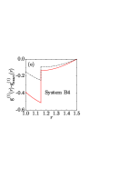
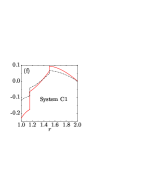
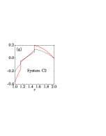
Figure 1: Difference $g^{(1)}(r)-g^{(1)}_{\text{exact}}(r)$ at $T^{=}1.5$ (solid lines) and $T^{*}=2$ (dash-dotted lines) for the systems described in Table 1.

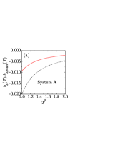
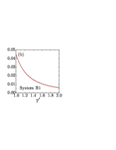
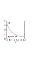
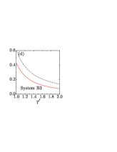
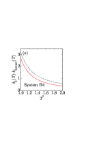
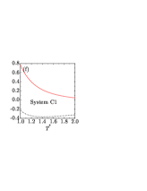
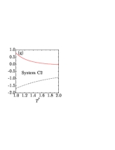
Figure 2: Differences $b_{3,v}(T^{*})-b_{3,\text{exact}}(T^{*})$ (solid lines) and $b_{3,c}(T^{*})-b_{3,\text{exact}}(T^{*})$ (dash-dotted lines) for the systems described in Table 1.

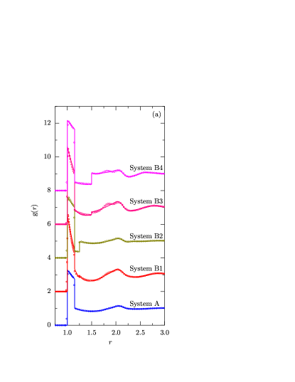
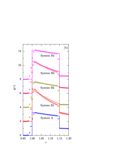
Figure 3: Comparison between the RDF as derived from the RFA (solid lines) and simulation data [11] (symbols) for systems A–B4 with $(T^{*},\rho^{*})=(1,0.6)$ (systems A, B2, and B4), $(2,0.9)$ (system B1), and $(1,0.9)$ (system B3). Panel (a) shows the region $0.75\leq r\leq 3$, while panel (b) magnifies the region $0.95\leq r\leq 1.20$. For better clarity, the data have been shifted upward two, four, six, and eight units for systems B1–B4, respectively.

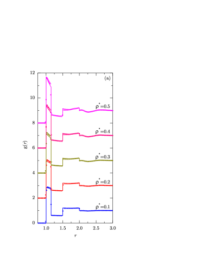
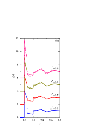
Figure 4: Comparison between the RDF as derived from the RFA (solid lines) and simulation data [11] (symbols) for system C2 with $T^{*}=1$ and (a) $\rho^{*}=0.1,\ldots,0.5$, (b) $\rho^{*}=0.6,\ldots,0.9$. For better clarity, in each panel the data have been successively shifted upward two units.

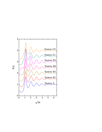
Figure 5: Plot of the structure factor $S(q)$ as derived from the RFA for systems A–C2 with $(T^{*},\rho)=(0.7,0.6)$. For better clarity, the data have been successively shifted upward half a unit.

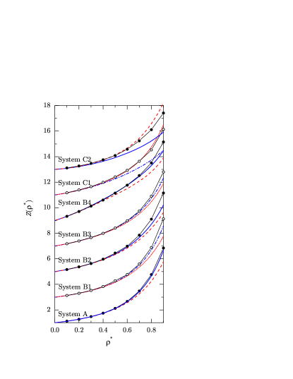
Figure 6: Comparison between the density-dependence of the compressibility factor as derived from the RFA (virial route: dashed and dotted lines, compressibility route: solid and dash-dotted lines) and simulation data [11] (symbols joined by lines) for systems A–C2 at $T^{*}=1.5$. For better clarity, the data have been successively shifted upward one unit.

Before comparing with simulation results, let us first consider the low-density behavior. Figure 1 displays the difference $g^{(1)}(r)-g^{(1)}_{\text{exact}}(r)$ at the reduced temperatures $T^{*}\equiv k_{B}T/|\epsilon_{1}|=1.5$ and $2$ for the systems of Table 1. We can observe that the deviations of the RFA values from the exact ones are rather small for the SW system A. In the SW+SS cases, the deviations tend to increase as one moves from system B1 to system B4. i.e., as the height and/or the range of the energy barrier increase. A similar behavior is observed in the SW+SS+SW (systems C1 and C2), this time by increasing the depth of the second well. Those deviations are substantially reduced if temperature increases. Interestingly, while the RFA overestimates $g^{(1)}(r)$ for system A, it underestimates it for systems B1–B4. In the case of systems C1 and C2, the difference $g^{(1)}(r)-g^{(1)}_{\text{exact}}(r)$ changes from negative to positive at a certain distance intermediate between $\lambda_{2}$ and $\lambda_{3}$. Regarding the jumps $\Delta g^{(1)}(\lambda_{j})$, we can observe that the RFA underestimates $\Delta g^{(1)}(1)$, yields the exact $\Delta g^{(1)}(\lambda_{n})$, and overestimates $\Delta g^{(1)}(\lambda_{j})$ for $1\leq j\leq n-1$ in systems B1–C2.

The deviations $b_{3,v}-b_{3,\text{exact}}$ and $b_{3,c}-b_{3,\text{exact}}$ are shown in Fig. 2 for the temperature range $1\leq T^{*}\leq 2$. As happened in Fig. 1, the magnitudes of those deviations generally decrease with growing temperature and increase when going from system A to system B4 and from system C1 to system C2. We have noted that this is generally the case not only for the absolute deviations but also for the relative ones. For instance, the magnitudes of the relative deviations of the pair $(b_{3,v},b_{3,c})$ with respect $b_{3,\text{exact}}$ at $T^{*}=1.5$ are $(0.1\%,0.2\%)$, $(0.3\%,0.3\%)$, $(1.6\%,1.9\%)$, $(2.7\%,4.4\%)$, $(6.6\%,9.1\%)$, $(2.7\%,5.8\%)$, and $(1.6\%,17.7\%)$ for systems A–C2, respectively. For system A, both $b_{3,v}$ and $b_{3,c}$ underestimate the exact values, while the opposite occurs for systems B1–B4. In the case of systems C1 and C2, $b_{3,v}$ overestimates $b_{3,\text{exact}}$ but $b_{3,c}$ underestimates it. The virial-route value $b_{3,v}$ is more accurate than the compressibility-route value $b_{3,c}$ in systems A–B4 and C2. In contrast, in the case of system C1, $b_{3,c}$ becomes more accurate than $b_{3,v}$ if $T^{*}>1.24$.

Now we turn to the comparison with the recent simulation data of Perdomo et al. [11], starting with the structural properties. In Fig. 3 we show the comparison between the results of the RFA approach for the RDF and the simulation values for systems A–B4 at different conditions of reduced density $\rho^{*}$ and reduced temperature $T^{*}$. There is clearly a very good agreement between the theoretical and the simulation results in all cases. On the other hand, Fig. 3(a) shows that in the chosen states of systems B3 and B4, the RFA does not capture some subtle details of the RDF in the interval $\lambda_{2}=1.5\leq r\leq 2$.

The general good agreement found in Fig. 3 is noteworthy for two reasons. First, taking into account that the values of the density are not small ($\rho^{*}=0.6$ and $0.9$, corresponding to $\eta=0.31$ and $0.47$, respectively), the agreement is clearly better than one might have expected in view of Figs. 1(a–e). Second, as said in Section 1, the simulation results do not correspond to genuine discontinuous potentials but to continuous potentials that mimic the discontinuous ones (see Ref. [11] for details). The latter feature manifests itself in the fact that, in contrast to the RFA results, the RDF simulation data do not present jumps at $r=\lambda_{j}$, as clearly seen in Fig. 3(b).

A more stringent test is carried out in Fig. 4, where the three-step system C2 is considered for the temperature $T^{*}=1$. A generally good agreement, comparable to the one already observed in Fig. 3, is present up to $\rho^{*}=0.6$. However, the agreement tends to deteriorate for the highest densities.

Within the RFA scheme, it is straightforward to obtain the static structure factor $S(q)$ through Eq. (6). In Fig. 5, we illustrate the behavior of $S(q)$ as a function of the wavenumber (divided by $2\pi$) at the state point $\rho^{*}=0.6$, $T^{*}=0.7$ for all cases listed in Table 1. As expected, $S(k)$ presents peaks at values of $q/2\pi$ around integer numbers, thus signaling the order induced by the hard-core diameter. In the particular case of system B4 (which corresponds to the highest and widest repulsive barrier), an “anomalous” local peak in the structure factor at $q/2\pi\sim 1/\lambda_{2}$ is clearly present. The existence of such a peak associated with competing interactions has been previously described [6]. In fact, in the case of SW+SS systems, the limits $T^{*}\to\infty$ and $T^{*}\to 0$ correspond to hard-sphere fluids of diameters $\sigma=1$ and $\lambda_{2}$, respectively. Thus, the local peak of $S(q)$ at $q/2\pi\sim 1/\lambda_{2}$ in system B4 becomes less pronounced as temperature increases and eventually disappears at about $T^{*}\simeq 0.9$ if $\rho=0.6$ (not shown).

After having analyzed the structural properties, we present in Fig. 6 the comparison between the results for the compressibility factor as a function of the reduced density $\rho^{*}$ computed using the RFA (taking both the virial and the compressibility routes) and the corresponding simulation data [11] at a reduced temperature $T^{*}=1.5$. One can observe that both RFA predictions agree well with the simulation data up to $\rho^{*}=0.6$ (systems A–B3) or $\rho^{*}=0.4$ (systems B4–C2). This represents a performance of the RFA better than expected from the behavior of the third virial coefficient in Fig. 2. In the high-density region ($\rho^{*}>0.6$) we see that both the RFA virial and compressibility routes tend to underestimate $Z$ in the case of the systems A–B4, what contrasts with the behavior observed in Fig. 2 for the third virial coefficient of systems B1–B4. On the other hand, in the case of the three-step systems C1 and C2, the virial (compressibility) route overestimates (underestimates) the compressibility factor, this time in qualitative agreement with Figs. 2(f,g). It is also quite apparent from Fig. 6 that the RFA compressibility route is more reliable than the RFA virial route for systems A–B4, but the opposite occurs for systems C1 and C2.

It should also be noted from Fig. 6 that, in all cases, when the values of the compressibility factor $Z$ obtained by the compressibility and virial RFA routes agree with each other, then they agree with the simulation results. This then provides a useful criterion to estimate the compressibility factor from the RFA method if simulation data are absent.

4 Concluding remarks

In this paper we have used the RFA approach introduced earlier for a general potential with a hard core and $n$-step constant sections [15] to compute the structural properties and the equation of state of a particular kind of discrete-potential fluids, namely the ones in which molecules interact via a potential consisting of a hard core plus up to three constant sections of different heights and widths, the middle one being a square shoulder. In the end, the method requires the (numerical) solution of $n=1$ (system A), $n=2$ (systems B1–B4), or $n=3$ (systems C1 and C2) coupled transcendental equations. In any case, being a semi-analytical nonperturbative method, the RFA naturally presents a clear advantage over other approaches, such as the usual integral equation method in the theory of liquids.

As a supplement to the results first derived in Ref. [15], we have obtained in this paper the RFA and exact analytical expressions of the RDF to first order in density and of the third virial coefficient for the general $n$-step interaction potential. The use of the RFA to find the equation of state of piecewise constant potentials is another contribution of the present work.

Apart from the comments made in the previous section concerning the cases we chose to illustrate our results, some additional remarks are in order. To begin with, the comparison with the most recent simulation data reinforces the conclusions drawn in our previous papers [15, 17], namely that the RFA approach is a valuable tool to compute the structural properties of fluids whose molecules interact via potentials consisting of a hard-core followed by one or more constant sections, except perhaps at low temperatures and high densities. In the present paper we have also shown that the compressibility factor of such systems derived with the RFA, using either the virial or the compressibility routes, is also reasonably accurate. While in principle one might try to obtain with the present approach also other thermodynamic properties, such as the liquid-vapor coexistence of these fluids, the heavy numerical work involved places this task outside the scope of this paper. Finally, the good agreement between our results for the RDF and the simulation data (obtained with an equivalent continuous potential) [11] suggests that, at least for the structural and thermodynamic properties, replacing discrete potentials with (appropriate) continuous ones [24] does not lead to serious errors.

CRediT authorship contribution statement

S. B. Yuste: Conceptualization, Methodology, Software, Formal analysis, Writing - Review & Editing, Funding acquisition A. Santos: Conceptualization, Methodology, Formal analysis, Writing - Review & Editing, Visualization, Funding acquisition M. López de Haro: Conceptualization, Methodology, Writing - Original Draft

Declaration of Competing Interest

The authors declare that they have no known competing financial interests or personal relationships that could have appeared to influence the work reported in this paper.

References

- [1] J. A. Barker, D. Henderson, What is “liquid”? Understanding the states of matter, Rev. Mod. Phys. 48 (1976) 587–671. doi:10.1103/RevModPhys.48.587.
- [2] G. Franzese, G. Malescio, A. Skibinsky, S. V. Buldyrev, H. E. Stanley, Generic mechanism for generating a liquid-liquid phase transition, Nature 409 (2001) 692–695. doi:10.1038/35055514.
- [3] A. Skibinsky, S. V. Buldyrev, G. Franzese, G. Malescio, H. E. Stanley, Liquid-liquid phase transitions for soft-core attractive potentials, Phys. Rev. E 69 (2004) 061206. doi:10.1103/PhysRevE.69.061206.
- [4] G. Malescio, G. Franzese, A. Skibinsky, S. V. Buldyrev, H. E. Stanley, Liquid-liquid phase transition for an attractive isotropic potential with wide repulsive range, Phys. Rev. E 71 (2005) 061504. doi:10.1103/PhysRevE.71.061504.
- [5] L. A. Cervantes, A. L. Benavides, F. del Río, Theoretical prediction of multiple fluid-fluid transitions in monocomponent fluids, J. Chem. Phys. 126 (2007) 084507. doi:10.1063/1.2463591.
- [6] I. Guillén-Escamilla, M. Chávez-Páez, R. Castañeda-Priego, Structure and thermodynamics of discrete potential fluids in the OZ-HMSA formalism, J. Phys.: Condens. Matter 19 (2007) 086224. doi:10.1088/0953-8984/19/8/086224.
- [7] A. B. de Oliveira, G. Franzese, P. A. Netz, M. C. Barbosa, Waterlike hierarchy of anomalies in a continuous spherical shouldered potential, J. Chem. Phys. 128 (2008) 064901. doi:10.1063/1.2830706.
- [8] A. B. de Oliveira, P. A. Netz, M. C. Barbosa, An ubiquitous mechanism for water-like anomalies, EPL 85 (2009) 36001. doi:10.1209/0295-5075/85/36001.
- [9] G. A. Chapela, S. E. Martínez-Casas, J. Alejandre, Molecular dynamics for discontinuous potentials. I. General method and simulation of hard polyatomic molecules, Mol. Phys. 53 (1984) 139–159. doi:10.1080/00268978400102181.
- [10] G. A. Chapela, L. E. Scriven, H. T. Davis, Molecular dynamics for discontinuous potential. IV. Lennard-Jonesium, J. Chem. Phys. 91 (1989) 4307–4313. doi:10.1063/1.456811.
- [11] R. Perdomo-Pérez, J. Martínez-Rivera, N. C. Palmero-Cruz, M. A. Sandoval-Puentes, J. A. S. Gallegos, E. Lázaro-Lázaro, N. E. Valadez-Pérez, A. Torres-Carbajal, R. Castañeda-Priego, Thermodynamics, static properties and transport behaviour of fluids with competing interactions, J. Phys.: Condens. Matter 34 (2022) 144005. doi:10.1088/1361-648X/ac4b29.
- [12] S. Hlushak, A. Trokhymchuk, S. Sokołowski, Direct correlation function of the square-well fluid with attractive well width up to two particle diameters, J. Chem. Phys. 130 (2009) 234511. doi:10.1063/1.3154583.
- [13] S. P. Hlushak, A. D. Trokhymchuk, S. Sokołowski, Direct correlation function for complex square barrier-square well potentials in the first-order mean spherical approximation, J. Chem. Phys. 134 (2011) 114101. doi:10.1063/1.3560049.
-
[14]
M. Bárcenas, G. Odriozola, P. Orea,
Propiedades
termodinámicas de fluidos de hombro/pozo cuadrado, Rev. Mex. Fís. 57
(2011) 485–490.
URL http://www.revistas.unam.mx/index.php/rmf/article/view/30601 - [15] A. Santos, S. B. Yuste, M. López de Haro, Rational-function approximation for fluids interacting via piece-wise constant potentials, Condens. Matter Phys. 15 (2012) 23602. doi:10.5488/CMP.15.23602.
- [16] A. Santos, A Concise Course on the Theory of Classical Liquids. Basics and Selected Topics, Vol. 923 of Lecture Notes in Physics, Springer, New York, 2016.
- [17] A. Santos, S. B. Yuste, M. López de Haro, M. Bárcenas, P. Orea, Structural properties of fluids interacting via piece-wise constant potentials with a hard core, J. Chem. Phys. 139 (2013) 074505. doi:10.1063/1.4818601.
- [18] J.-P. Hansen, I. R. McDonald, Theory of Simple Liquids, 4th Edition, Academic Press, London, 2013.
- [19] S. B. Yuste, A. Santos, Radial distribution function for hard spheres, Phys. Rev. A 43 (1991) 5418–5423. doi:10.1103/PhysRevA.43.5418.
- [20] S. B. Yuste, A. Santos, A model for the structure of square-well fluids, J. Chem. Phys. 101 (1994) 2355–2364. doi:10.1063/1.467676.
- [21] S. B. Yuste, M. López de Haro, A. Santos, Structure of hard-sphere metastable fluids, Phys. Rev. E 53 (1996) 4820–4826. doi:10.1103/PhysRevE.53.4820.
- [22] A. Santos, S. B. Yuste, M. López de Haro, Structural and thermodynamic propertiesof hard-sphere fluids, J. Chem. Phys. 153 (2020) 120901. doi:10.1063/5.0023903.
- [23] J. Abate, W. Whitt, The Fourier-series method for inverting transforms of probability distributions, Queueing Syst. 10 (1992) 5–88. doi:10.1007/BF01158520.
- [24] J. Munguía-Valadez, M. A. Chávez-Rojo, E. J. Sambriski, J. A. Moreno-Razo, The generalized continuous multiple step (GCMS) potential: model systems and benchmarks, J. Phys.: Condens. Matter 34 (2022) 184002. doi:10.1088/1361-648X/ac4fe8.