Running coupling and non-perturbative corrections for O$(N)$ free energy and for disk capacitor

Abstract

We reconsider the complete solution of the linear TBA equation describing the energy density of finite density states in the $O(N)$ nonlinear sigma models by the Wiener-Hopf method. We keep all perturbative and non-perturbative contributions and introduce a running coupling in terms of which all asymptotic series appearing in the problem can be represented as pure power series without logs. We work out the first non-perturbative contribution in the $O(3)$ case and show that (presumably because of the instanton corrections) resurgence theory fails in this example. Using the relation of the $O(3)$ problem to the coaxial disks capacitor problem we work out the leading non-perturbative terms for the latter and show that (at least to this order) resurgence theory, in particular the median resummation prescription, gives the correct answer. We demonstrate this by comparing the Wiener-Hopf results to the high precision numerical solution of the original integral equation.

1 Introduction

Quantum chromodynamics (QCD), the theory of the strong interaction is asymptotically free in perturbation theory and there is a dynamically generated mass scale. The nature of the perturbative expansion is asymptotic, which manifests itself in the factorially growing coefficients. This factorial growth can be tamed by switching to the Borel plane, i.e. by analysing the perturbative coefficients divided by the appropriate factorials. The perturbative expansion of the various observables on the Borel plane then has a finite radius of convergence and exhibits singularities typically on the real line. Singularities on the positive real line prevent Borel summability, leading to non-perturbative ambiguities. These ambiguities can originate from instantons and/or renormalons Beneke:1998ui ; Bauer:2011ws . The full knowledge of the singularities, in principle, enables one to formulate an ambiguity free trans-series for each observable. It would be ideal to proceed along these lines for QCD, however, only a very limited number of perturbative terms are at our disposal. Thus, exactly soluble models with properties similar to QCD have been becoming more and more important.

There are various toy models in two dimensions that share many physically relevant aspects with QCD, but are nevertheless exactly soluble. They provide ideal testing grounds of non-perturbative physics. Particularly interesting are the asymptotically free theories with a dynamically generated mass gap. By coupling an external field to one of the conserved charges the free energy can be calculated in two alternative ways: from perturbation theory based on the UV Lagrangean and also from the thermodynamic limit of the Bethe ansatz, which uses the IR degrees of freedom, the masses and scatterings of particles.

In the UV description the singular point of the renormalized running coupling defines a non-perturbative scale, $\Lambda$, which appears in the perturbative expansion. On the IR side the expansion is based on the Wiener-Hopf technique and includes the physical mass of the particles. By matching the two expansions the highly non-trivial $m/\Lambda$ mass gap relation can be established. This calculation was first performed in the $O(N)$ models Hasenfratz:1990ab ; Hasenfratz:1990zz and later it was extended for various other two dimensional integrable models: for the Gross-Neveu model Forgacs:1991rs ; Forgacs:1991ru , for the chiral $SU(N)\times SU(N)$ model Balog:1992cm , for their supersymmetric extensions Evans:1994sv ; Evans:1994sy and also for the sine-Gordon model Zamolodchikov:1995xk . This calculation involves only the first few perturbative coefficients. It is notoriously difficult to expand the TBA equations to higher orders and the next order result, decisive for the AdS/CFT correspondence, was obtained in the $O(N)$ models by direct perturbative calculations Bajnok:2008it .

A breakthrough in this field was achieved by Volin Volin:2009wr ; Volin:2010cq , who managed in the $O(N)$ models to transform the expansion of TBA into algebraic relations and to calculate the first 26 perturbative coefficients. These were enough to see the factorial growth and to locate the leading singularities on the Borel plane. His approach was extended to other relativistic Marino:2019eym and non-relativistic models Marino:2019fuy ; Marino:2020dgc ; Marino:2020ggm ; Reichert:2020ymc . By focusing on the $O(3)$ and $O(4)$ models and performing the calculations numerically, one can even obtain $336/2000$ perturbative terms, respectively Abbott:2020mba ; Abbott:2020qnl ; Bajnok:2021zjm . Alternatively, one can make a systematic large $N$ expansion of the TBA equations, which can be matched to large $N$ renormalon diagrams DiPietro:2021yxb ; Marino:2021six .

Having enough perturbative coefficients fixes the leading factorial and sub-factorial growths, which determine the nature and locations of the closest Borel singularities. These singularities give rise to non-perturbative corrections. The theory which connects the asymptotic behaviour of the perturbative series to the non-perturbative corrections is called resurgence, see Aniceto:2018bis ; Dorigoni:2014hea for modern reviews and references therein. In its strongest version it implies that the perturbative coefficients determine all the non-perturbative corrections. By taking into account all the non-perturbative corrections the physical observables can be written into trans-series forms. A trans-series is a series containing all exponentially suppressed non-perturbative corrections, where each term is multiplied with an (asymptotic) perturbative series. It is understood to be Borel resummed laterally and the various non-perturbative terms ensure that it is ambiguity free. The first few terms of the trans-series were determined and matched to the numerical solution of the TBA equation for the $O(4)$ model in Abbott:2020mba ; Abbott:2020qnl , while the leading order results were analytically proven in Bajnok:2021dri . Particularly important are the bridge equations which could relate the perturbative expansions of the various non-perturbative terms to each other. A big leap in this direction was the systematic expansion of the TBA equation, which provided pertubative expansion of the various non-perturbative contributions in parallel Marino:2021dzn . The aim of our paper is to extend and to elaborate this approach for the $O(N)$ models in many respects.

One of our main results is the introduction of the running coupling on the TBA side in the $O(N)$ models, similarly to how it appeared for the Gross-Neveu model in Forgacs:1991rs ; Forgacs:1991ru . In the TBA formulation, the external field, $h$, forces the negatively charged particles to condense into the $h$-dependent rapidity interval $[-B,B]$. The rapidity density can be determined from the TBA integral equation based on the scattering matrix, and provides the density $\rho$ and energy density $\epsilon$. Large $h$ corresponds to large $B$ and the systematic expansion goes in $B^{-1}$ multiplied with a polynomial in $\log B$. Since $\epsilon/\rho^{2}$ is related to the free energy, it can be expanded purely in powers of the Lagrangean’s running coupling, $\alpha$. This is, however, not expected either from $\rho$ or from $\epsilon$ and one of our main result is the introduction such a running coupling, $v$, in which they can be expanded as a power series, i.e. without $\log v$. The main advantage of this running coupling becomes obvious when we analyse models, which are mathematically equivalent, but physically different from the $O(N)$ sigma models. In particular, for $N=3$ the integral equation is the same which determines the groundstate energy in the Lieb-Liniger model lieb1963exact . It is also equivalent to the Love equation, which describes the circular plate capacitor Love:1949 .

The Maxwell-Kirchhoff disk capacitor problem is to calculate the capacitance of two, oppositely charged, infinitely thin coaxial conducting disks of radius $a$ and distance $d$. The leading order behaviour for small $\kappa=d/a$ can be calculated easily, but subleading corrections are very involved and challenged many prominent physicists. The expansion involves powers and logarithms of $\kappa$ and is very difficult to obtain systematically. The exact analytical description was provided by Love and the kernel of his integral equation is the same which appears in the O(3) sigma model. Adaptation of Volin’s method allowed to generate many perturbative terms Marino:2019fuy ; Reichert:2020ymc , but non-perturbative corrections have not been analyzed yet although the first non-perturbative correction was given in Marino:2019fuy for the closely related Lieb-Liniger model. Our aim is to connect the capacitance to the observables of the O(3) sigma model and analyze its non-perturbative corrections.

The O(3) model is interesting in its own right as the leading exponentially suppressed (in perturbation theory) terms are not related to the asymptotics of the perturbative coefficients Marino:2021dzn ; Bajnok:2021zjm . We revisit also this model and, by exploiting our simplified equations, we investigate this anomalous behaviour in detail.

The paper is organized as follows: in the rest of this section we first recall the interesting history of the capacitor problem. We then introduce the form of the integral equations we are dealing with together with various observables of relevance and establish a relationship between them. In particular, the capacitance of the circular plate capacitor will be related to the density and energy density of the $O(3)$ sigma model. In section 2 we recall the Wiener-Hopf method developed to solve the integral equation and present also a useful simplification, which leads to the introduction of the running coupling. By separating the singularities of the integral kernel we present a form that allows systematic calculations of the various non-perturbative corrections. We then comment on the structure of these non-perturbative corrections and the resurgence properties of the perturbative expansion. As the $O(3)$ kernel is drastically different from the $N\geq 4$ cases we analyse it more carefully. Section 3 is devoted to the calculation of the leading exponential corrections in the $O(3)$ sigma model, while Section 4 focuses on the non-perturbative analysis of the circular plate capacitor. Our conclusions are summarized in section 5. The paper is closed by several Appendices. In Appendix A we introduce our notations and the building blocks for the Wiener-Hopf analysis. Appendix B provides details on the integral equation when the source is a constant function. In Appendix C we calculate explicitly the first two orders based on the relationship between the various observable we found earlier and by introducing a new analytical tool. Here we elaborate on how the Laplace transformation can be used to solve explicitly the expansion of the integral equation. Finally, in Appendix D, we explain how Volin’s algorithm can be used to calculate the perturbative expansion in our running coupling.

The contribution of one of the authors of Ref. Balog:1992cm , Ferenc Niedermayer, was essential in obtaining the analytic solutions presented in appendix C. We devote this paper to the memory of Ferenc.

1.1 The Maxwell-Kirchhoff disk capacitor problem

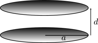
Figure 1: Geometry of the parallel disks capacitor.

The problem is to calculate the capacity of two, infinitely thin coaxial conducting disks of radius $a$ and distance $d$ (see Fig. 1). If the disks are kept at fixed potential $\pm U$ (equal and opposite) the task is to solve this boundary value problem of electrostatics, determine the electric field around the two disks and the charge distribution on the disks and finally calculate the capacity $C_{\rm phys}$ of the arrangement.

The solution is not available in closed form but there are results in the limit of small separation of the disks. If

$$\kappa=\frac{d}{a}$$ (1.1)

is small, the problem reduces to the high-school problem of infinite parallel conducting plates, the electric field becomes constant between the plates and the capacity per unit surface area becomes

$$\frac{C_{\rm phys}}{a^{2}\pi}=\frac{\epsilon_{0}}{d},$$ (1.2)

where $\epsilon_{0}$ is the vacuum permittivity.

If we want to go beyond this approximation, the effect of the edges of the disks has to be taken into account. This legendary problem of electrostatics attracted the attention of many prominent physicists in the last one and a half century. The saga started by Maxwell maxwell who was the first to study the edge effects.

Introducing the dimensionless quantity

$${\cal C}=\frac{1}{4\pi\epsilon_{0}a}C_{\rm phys}$$ (1.3)

its $\kappa\to 0$ asymptotic expansion can be written as

$${\cal C}=\frac{1}{4\kappa}+\frac{\mathsf{L}-1}{4\pi}+\frac{\kappa}{16\pi^{2}}({\mathsf{L}}^{2}-2)+O(\kappa^{2}),$$ (1.4)

where $\mathsf{L}=\ln(16\pi/\kappa)$. Here the first term is the high-school result and the next (NLO) term was found by Kirchhoff kirchhoff1877theorie by a heuristic derivation (based on earlier result of Clausius and Helmholtz). Much later Ignatowsky ignatowsky1931kreisscheibenkondensator claimed the constant in the NLO term should be replaced as

$$\ln\frac{16\pi}{e}\rightarrow\ln\frac{8}{\sqrt{e}}.$$ (1.5)

This turned out to be incorrect, however, curiously, Pólya and Szegő polya1945inequalities proved that the sum of the first two terms with this modified constant gives an exact lower bound for the capacity!

Love Love:1949 derived the integral equation (4.2) describing the problem and Hutson hutson1963circular proved rigorously from the Love equation that Kirchhoff’s NLO result was correct. Actually, Love’s equation already appeared in a much earlier paper hafen1910studien . Sneddon sneddon1966mixed simplified the derivation of Love’s equation and proved the existence and uniqueness of its solution. (For a recent elementary derivation, see Felderhof:2013 .)

Nearly a century after Kirchhoff’s result the NNLO $\ln^{2}$ term was calculated Leppington:1970 . The full NNLO calculation of shaw1970circular was improved and corrected by wigglesworth1972comments ; chew1982microstrip .

The Lieb-Liniger model describes the system of one-dimensional bosons interacting with a repulsive $\delta$-potential lieb1963exact . This non-relativistic system is described by Lieb’s integral equation. Gaudin gaudin1971boundary pointed out first that Love’s and Lieb’s integral equations are identical and used potential theory to calculate the NLO term in the free energy of the Lieb-Liniger model. For a comprehensive review of the mathematics and physical applications of the Love-Lieb integral equation, see Farina:2020zlr .

It was noted in Hasenfratz:1990zz that the TBA integral equation describing the free energy of the $O(3)$ non-linear sigma model in an external field is also closely related to Love’s equation. Thus these three completely distinct physical systems are all described by the same mathematics.

Systematic asymptotic expansion of the integral equations (following Maxwell’s original ideas) was based (using the disk language) on the method of “matched” asymptotic expansions of the potential near and away from the edges. The first few terms in the asymptotic expansion were calculated in lieb1963exact ; popov1977theory ; hutson1963circular . This method was elegantly extended to all orders, for the $O(N)$ free energy, by Volin Volin:2009wr ; Volin:2010cq . Volin’s method was adapted to the disk problem in Marino:2019fuy . In Reichert:2020ymc the small $\kappa$ expansion of ${\cal C}$ was given explicitly up to $O(\kappa^{7})$.

Numerical studies of the integral equation were initiated in nystrom1930praktische ; nomura ; cooke1956solution ; cooke1958coaxial and continued with ever greater precision norgren2009capacitance ; paffuti2017numerical ; paffuti2019galerkin .

In this paper we study the disk problem using its relation to the free energy of the $O(3)$ model and introduce a running coupling $\beta$ by

$$\frac{2\pi}{\kappa}=\frac{1}{\beta}+\ln\beta-\ln\frac{8}{e}$$ (1.6)

in terms of which the capacity can be compactly written as an asymptotic power series, see (4.8).

1.2 Integral equations and observables

In this paper we analyze linear integral equations of the form

$$\chi_{i}(\theta)-\int_{-B}^{B}d\theta^{\prime}K(\theta-\theta^{\prime})\chi_{i}(\theta^{\prime})=r_{i}(\theta),\qquad\quad-B\leq\theta\leq B,$$ (1.7)

where the kernel $K(\theta)$ and the sources $r_{i}(\theta)$ are symmetric functions of $\theta$, implying the same for the solutions, too. These solutions $\chi_{i}(\theta)$ depend implicitly on $B$, but we suppress this $B$-dependence in the notation.

Observe that the $B$-derivative of $\chi_{i}(\theta)$, which we denote by a dot, $\partial\chi_{i}(\theta)/\partial B=\dot{\chi}_{i}(\theta)$, satisfies the same type of equation

$$\dot{\chi}_{i}(\theta)-\int_{-B}^{B}d\theta^{\prime}K(\theta-\theta^{\prime})\dot{\chi}_{i}(\theta^{\prime})=R_{i}(\theta)$$ (1.8)

with the source term

$$R_{i}(\theta)=\left[K(\theta-B)+K(\theta+B)\right]\chi_{i}(B),$$ (1.9)

which is again symmetric in $\theta$.

We are interested in observables of the form

$$O_{ij}=\int_{-B}^{B}\frac{d\theta}{2\pi}\chi_{i}(\theta)r_{j}(\theta),$$ (1.10)

where we again suppressed the $B$-dependence of $O_{ij}$ and will do so if it does not lead to any confusion. The symmetry of the kernel and the integral equation implies that $O_{ij}$ is symmetric in $i,j$. Actually, not all $O_{ij}$ are independent as they can be expressed in terms of $\chi_{i}(B)$ and integration constants, which follows from the key formula

$$\dot{O}_{ij}\equiv\frac{\partial O_{ij}}{\partial B}=\frac{1}{\pi}\chi_{i}(B)\chi_{j}(B).$$ (1.11)

This nice expression can be derived by observing that

$$\dot{O}_{ij} =\frac{1}{\pi}\chi_{i}(B)r_{j}(B)+\int_{-B}^{B}\frac{d\theta}{2\pi}\dot{\chi}_{i}(\theta)r_{j}(\theta)$$ (1.12)

and by exploiting that the second term is of the form of $O_{ij}$. Its symmetry implies that $\int_{-B}^{B}\frac{d\theta}{2\pi}\dot{\chi}_{i}(\theta)r_{j}(\theta)=\int_{-B}^{B}\frac{d\theta}{2\pi}\chi_{j}(\theta)R_{i}(\theta)$ thus we can recognize the appearance of $\chi_{j}(B)=\chi_{j}(-B)$ leading to the required conclusion (1.11).

In this paper we analyze the two dimensional $O(N)$ sigma model in a magnetic field. The kernel

$$K(\theta)=\frac{1}{2\pi i}\partial_{\theta}\log S(\theta)$$ (1.13)

is the logarithmic derivative of the scattering matrix

$$S(\theta)=-\frac{\Gamma(\frac{1}{2}-\frac{i\theta}{2\pi})\Gamma(\Delta-\frac{i\theta}{2\pi})\Gamma(1+\frac{i\theta}{2\pi})\Gamma(\frac{1}{2}+\Delta+\frac{i\theta}{2\pi})}{\Gamma(\frac{1}{2}+\frac{i\theta}{2\pi})\Gamma(\Delta+\frac{i\theta}{2\pi})\Gamma(1-\frac{i\theta}{2\pi})\Gamma(\frac{1}{2}+\Delta-\frac{i\theta}{2\pi})},$$ (1.14)

where the parameter $\Delta$ is related to $N$ as $1/\Delta=N-2$.

We are interested in two problems: In the first, the source of the integral equation is $r_{c}(\theta)=\cosh\theta$, while in the second it is simply $r_{1}(\theta)=1$. The physical meaning of $m\chi_{c}(\theta)$ is the rapidity density of particles in the groundstate. The density and energy density are simply

$$\rho=mO_{c1}=m\int_{-B}^{B}\frac{d\theta}{2\pi}\chi_{c}(\theta)\quad;\qquad\epsilon=m^{2}O_{cc}=m^{2}\int_{-B}^{B}\frac{d\theta}{2\pi}\chi_{c}(\theta)\cosh\theta,$$ (1.15)

which defines a one-to-one correspondence between $\rho$ and $B$. They are fixed by the magnetic field, through $h=\partial_{\rho}\epsilon=\dot{\epsilon}/\dot{\rho}$, which follows from minimising the free energy over $\rho$. Alternatively, one can determine directly the free energy ${\cal F}(h)=m^{2}O_{cc}-hmO_{c1}$ as a function of $h$, where $B$ is expressed with $h$ from $h\chi_{1}(B)=m\chi_{c}(B)$.

We will pay particular attention to the case $\Delta=1$, i.e. to the $O(3)$ model, where the kernel is a simple rational function $K(\theta)=1/(\theta^{2}+\pi^{2})$. As we discussed above, the corresponding integral equation shows up in two unrelated but interesting problems, namely in the Lieb-Liniger model and in the circular disk capacitor. In the capacitor problem the relevant observable is the capacity (as a function of $B$), which is simply related to

$$O_{11}=\int_{-B}^{B}\frac{d\theta}{2\pi}\chi_{1}(\theta).$$ (1.16)

In view of (1.11), the first and the second problems with solutions $\chi_{c}(\theta)$ and $\chi_{1}(\theta)$ are not independent. The knowledge of any of them determines the 3 independent integrals up to integration constants, e.g.

$$\dot{O}_{11}=\frac{\dot{O}_{c1}^{2}}{\dot{O}_{cc}}$$ (1.17)

2 Wiener-Hopf method and running coupling

In this section we present a solution of the TBA integral equations (1.7) following the Wiener-Hopf method. We restrict our consideration to the case of the $O(N)$ non-linear sigma models and in particular the $O(3)$ model. Our derivation is very similar to that of Hasenfratz:1990zz ; Hasenfratz:1990ab ; Marino:2021dzn but here we concentrate on the introduction and use of running couplings, which are useful in presenting perturbative series.

Many of the technical details and various definitions and results are collected in appendix A.

2.1 Derivation of the Wiener-Hopf equations

Let us temporarily suppress the $c,1$ indices and extend the TBA equation (1.7) to all $\theta$ as follows.

$$\chi(\theta)-\int_{-\infty}^{\infty}K(\theta-\theta^{\prime})\chi(\theta^{\prime})d\theta^{\prime}=r(\theta)+R(\theta)+L(\theta).$$ (2.1)

Here we extended $\chi(\theta)$ and $r(\theta)$ by defining

$$\chi(\theta)=r(\theta)=0,\qquad\quad|\theta|>B$$ (2.2)

and added $R(\theta)$ and $L(\theta)$ satisfying

$$R(\theta)=0,\quad\theta\leq B;\qquad\qquad L(\theta)=R(-\theta).$$ (2.3)

Next we use the Fourier transformed functions $\tilde{\chi}(\omega)$, $\tilde{r}(\omega)$, $\tilde{R}(\omega)$ to define

$$X_{+}(\omega)=e^{-i\omega B}\tilde{R}(\omega),\quad r_{\pm}(\omega)=e^{\pm i\omega B}\tilde{r}(\omega),\quad\chi_{\pm}(\omega)=e^{\pm i\omega B}\tilde{\chi}(\omega),\quad X_{-}(\omega)=X_{+}(-\omega).$$ (2.4)

$r_{\pm}$ and $\chi_{\pm}$ are analytic everywhere and vanish for large $|\omega|$ in the upper/lower complex half-planes $H_{\pm}$, whereas $X_{\pm}$ are analytic in $H_{\pm}$ and vanish there for large $|\omega|$.

$$Q_{\pm}(\omega)=G_{\pm}(\omega)X_{\pm}(\omega),\qquad\quad Q_{-}(\omega)=Q_{+}(-\omega)$$ (2.5)

have similar properties, see (A.3) and (A.4).

Going to Fourier space the extended TBA equation (2.1) becomes

$$[1-\tilde{K}(\omega)]\tilde{\chi}(\omega)=\tilde{r}(\omega)+\tilde{R}(\omega)+\tilde{L}(\omega),$$ (2.6)

which can be rearranged as ($\alpha(\omega)$ is defined by (A.9))

$$\frac{\chi_{+}}{G_{+}}=G_{-}r_{+}+\alpha Q_{+}+Q_{-}.$$ (2.7)

Decomposing it into negative and positive parts, we get the following two equations

$$Q_{-}+(\alpha Q_{+})^{(-)}+(G_{-}r_{+})^{(-)}=0,$$ (2.8)

$$\frac{\chi_{+}}{G_{+}}=(\alpha Q_{+})^{(+)}+(G_{-}r_{+})^{(+)}.$$ (2.9)

We now spell out the first of these for $\omega=-2i\xi$ and use $Q_{-}(\omega)=Q_{+}(-\omega)$. We obtain

$$Q_{+}(2i\xi)+\frac{1}{2\pi}\int_{-\infty}^{\infty}\frac{\alpha(\omega)Q_{+}(\omega)}{2\xi-i\omega}d\omega+\frac{1}{2\pi}\int_{-\infty}^{\infty}\frac{G_{-}(\omega)r_{+}(\omega)}{2\xi-i\omega}d\omega=0.$$ (2.10)

Similarly, the second equation for $\omega=i\kappa$ becomes

$$\chi_{+}(i\kappa)=G_{+}(i\kappa)\left\{\frac{1}{2\pi}\int_{-\infty}^{\infty}\frac{\alpha(\omega)Q_{+}(\omega)}{\kappa+i\omega}d\omega+\frac{1}{2\pi}\int_{-\infty}^{\infty}\frac{G_{-}(\omega)r_{+}(\omega)}{\kappa+i\omega}d\omega\right\}.$$ (2.11)

It is sufficient to know $\chi_{+}$ along the positive imaginary axis, since the two density integrals

$$O_{.c}=\frac{1}{2\pi}\int_{-\infty}^{\infty}\chi(\theta)\cosh\theta d\theta\quad{\rm and}\quad O_{.1}=\frac{1}{2\pi}\int_{-\infty}^{\infty}\chi(\theta)d\theta$$ (2.12)

are given by

$$O_{.c}=\frac{e^{B}}{2\pi}\chi_{+}(i)\qquad{\rm and}\qquad O_{.1}=\frac{1}{2\pi}\chi_{+}(0)$$ (2.13)

and using the Cauchy integral

$$\chi_{+}(i\kappa)=\frac{1}{2\pi i}\int_{-\infty}^{\infty}\frac{\chi_{+}(\omega)d\omega}{\omega-i\kappa}$$ (2.14)

the boundary value $\chi(B)$ can also be obtained from

$$\chi(B)=\lim_{\kappa\to\infty}\kappa\chi_{+}(i\kappa).$$ (2.15)

So far we reviewed the standard way Hasenfratz:1990zz ; Hasenfratz:1990ab ; Marino:2021dzn of applying the Wiener-Hopf method to the $O(N)$ nonlinear sigma model. In the rest of this section we will follow a novel way of analyzing the problem by slightly rearranging the terms in the integral equation (2.10) allowing us to introduce running couplings already at an early stage of the calculation.

Technically, it is very difficult to extract the particle density $O_{c1}$ using (2.13) as the kernels are singular at the origin. An alternative way to obtain the particle density $O_{c1}$ is to go back to the original TBA equation (2.6) for the $\chi_{c}$ problem and use the small $|\omega|$ expansions

$$1-\tilde{K}(\omega)=\pi\Delta|\omega|+O(\omega^{2}),\quad\tilde{\chi}_{c}(\omega)=2\pi O_{c1}+O(\omega^{2}),\quad\tilde{r}_{c}(\omega)=2\sinh B+O(\omega^{2}),$$ (2.16)

together with the small $|\omega|$ expansion of $\tilde{R}(\omega)$, which is analytic in the upper half plane only:

$$\tilde{R}(\omega)=a-ib\omega-ic\omega\ln(-i\omega)+O(|\omega|^{2}),$$ (2.17)

where $a$, $b$, $c$ are some constants. Here, and also throughout this paper, the symbol $O(x^{p})$ includes possible logarithmic terms of the form $x^{p}(\ln x)^{q}$. Using $\tilde{L}(\omega)=\tilde{R}(-\omega)$, for real $\omega$ we find

$$\tilde{R}(\omega)+\tilde{L}(\omega)=2a-\pi c|\omega|+O(|\omega|^{2})$$ (2.18)

and using (2.6) we can determine

$$a=-\sinh B,\qquad\quad c=-2\pi\Delta O_{c1}.$$ (2.19)

Thus the value of the particle density $O_{c1}$ is hidden in the small $\omega$ expansion of $\tilde{R}$.

Since it is difficult to perform this small $\omega$ expansion or to evaluate (2.11) at the singular point $\kappa=0$, we will solve both problems ($\chi_{c}$ and $\chi_{1}$) and calculate the densities from

$$O_{cc}=\frac{e^{B}}{2\pi}\chi_{c+}(i),\qquad\quad O_{c1}=O_{1c}=\frac{e^{B}}{2\pi}\chi_{1+}(i).$$ (2.20)

Finally, $O_{11}$ will be obtained (up to an integration constant) using (1.17). This way we only use (2.11) for $\kappa=1$ and $\kappa=\infty$, which are well defined.

2.2 The $\chi_{c}$ problem

In this case

$$r_{c+}(\omega)=\frac{1}{2}e^{2i\omega B}\left(\frac{e^{B}}{1+i\omega}+\frac{e^{-B}}{i\omega-1}\right)+\frac{1}{2}\left(\frac{e^{B}}{1-i\omega}-\frac{e^{-B}}{1+i\omega}\right).$$ (2.21)

It is useful to introduce the new unknown $q_{+}(\omega)$ by

$$Q_{+}(\omega)+\frac{G_{+}(\omega)}{2}\left(\frac{e^{B}}{1+i\omega}+\frac{e^{-B}}{i\omega-1}\right)=\frac{e^{B}G_{+}(i)}{2}q_{+}(\omega)$$ (2.22)

because then the first term in (2.21) can be absorbed into the integral containing $\alpha(\omega)$ and the contribution of the second term of (2.21) can be explicitly integrated in (2.10) by closing the integration contour at infinity in $H_{-}$. We obtain

$$q_{+}(2i\xi)+\frac{1}{2\pi}\int_{-\infty}^{\infty}\frac{\alpha(\omega)q_{+}(\omega)}{2\xi-i\omega}d\omega=\frac{1}{1-2\xi}.$$ (2.23)

Manipulating (2.11) similarly, we get

$$O_{cc}=\frac{e^{2B}G_{+}^{2}(i)}{8\pi}W,\qquad\quad\chi_{c}(B)=\frac{e^{B}G_{+}(i)}{2}w,$$ (2.24)

where

$$W=1+\frac{1}{\pi}\int_{-\infty}^{\infty}\frac{\alpha(\omega)q_{+}(\omega)}{1+i\omega}d\omega,\qquad\qquad w=1+\frac{1}{2\pi}\int_{-\infty}^{\infty}\alpha(\omega)q_{+}(\omega)d\omega.$$ (2.25)

We note that using (2.17) and (A.4) we can derive the small $|\omega|$ expansion

$$\frac{e^{B}G_{+}(i)}{2}q_{+}(\omega)=\frac{\sqrt{-i\omega}}{\sqrt{\pi\Delta}}[b_{1}+c\ln(-i\omega)+O(|\omega|)],\qquad b_{1}=b-B\sinh B+\cosh B.$$ (2.26)

The introduction of the new variable $q_{+}$ simplifies the equations but the price to pay is that $q_{+}$ is no longer analytic in $H_{+}$: it has a pole at $\omega=i$. Sometimes it is useful to remove this pole term and write

$$q_{+}(2i\xi)=k_{+}(2i\xi)+\frac{1}{1-2\xi},$$ (2.27)

where $k_{+}$ is analytic in $H_{+}$.

Figure 2: The ${\cal C}_{LR}$ contour.

The next step in the Wiener-Hopf analysis is the deformation of the contour of the $\omega$ integration. Using the fact that $\alpha q_{+}$ is analytic in $H_{+}$ except on the imaginary axis, we deform the $\omega$ contour to ${\cal C}_{LR}$, which is defined as coming down from infinity to zero slightly to the left along the imaginary axis and then going up to infinity slightly to right of the imaginary axis (see Fig. 2):

$$q_{+}(2i\xi)+\frac{i}{2\pi}\int_{{\cal C}_{LR}}\frac{\alpha(2i\xi^{\prime})q_{+}(2i\xi^{\prime})}{\xi+\xi^{\prime}}d\xi^{\prime}=\frac{1}{1-2\xi}.$$ (2.28)

The contribution of the poles at $\xi=\xi_{\ell}$ (see appendix A) to this integral cancel due to the opposite signs in (A.23) for the left and right integrals. In this region the integration along ${\cal C}_{LR}$ reduces to the principal value integral of the discontinuity. The pole of $q_{+}$ at $\xi=1/2$ only contributes for $N=3$, since for larger $N$ the function $\alpha$ vanishes at this point. Using (A.15), (2.28) simplifies to

$$q_{+}(2i\xi)+\frac{\delta_{N,3}}{e}\,\frac{e^{-2B}}{1+2\xi}+\frac{1}{\pi}{\cal P}\int_{0}^{\infty}\frac{e^{-4B\xi^{\prime}}\beta(\xi^{\prime})q_{+}(2i\xi^{\prime})}{\xi+\xi^{\prime}}d\xi^{\prime}=\frac{1}{1-2\xi}.$$ (2.29)

For the $W$ integral in (2.25) the contribution of the $\xi=\xi_{\ell}$ poles also cancels, but the region around $\xi=1/2$ must be treated carefully. Using the results (A.24-A.26) we obtain

$$W=1+2\Lambda_{o}e^{-2B}+\frac{4}{\pi}{\cal P}\int_{0}^{\infty}\frac{e^{-4B\xi}\beta(\xi)q_{+}(2i\xi)}{1-2\xi}d\xi,$$ (2.30)

where

$$\Lambda_{o}=\left\{\begin{matrix}-\frac{1}{2}\sin\frac{\pi\gamma_{1}}{2}\tilde{h}_{1}\qquad\quad&N\geq 4,\\ \frac{1}{e}(2B+k_{+}(i)+1-\gamma_{E}-\ln 2)\qquad\quad&N=3.\end{matrix}\right.$$ (2.31)

Here $\tilde{h}_{1}$ is defined by (A.26) and for $N=3$

$$k_{+}(i)=-\frac{1}{2e}e^{-2B}-\frac{2}{\pi}{\cal P}\int_{0}^{\infty}\frac{e^{-4B\xi}\beta(\xi)q_{+}(2i\xi)}{1+2\xi}d\xi.$$ (2.32)

Finally evaluating $w$ in (2.25) gives

$$w=1+\frac{\delta_{N,3}}{e}e^{-2B}+\frac{2}{\pi}{\cal P}\int_{0}^{\infty}e^{-4B\xi}\beta(\xi)q_{+}(2i\xi)d\xi.$$ (2.33)

Following Marino:2021dzn we now introduce the integration along the contour ${\cal C}_{+}$, which goes from $0$ to $\infty$ slightly to the left of the imaginary axis (in the variable $2i\xi$). In terms of $\xi$ this is slightly above the real axis. The reason to use this integration path is that it resembles the $+$ lateral Borel resummation. We introduce this new integration using the rule

$$\int_{{\cal C}_{+}}=-i\pi\sum_{{\rm res}}+{\cal P}\int.$$ (2.34)

Here in front of the sum of residues term we have the factor $-i\pi$ because the integral near the poles is only a half-circle and its orientation is clock-wise. (2.29) becomes

$$q_{+}(2i\xi)+\frac{\delta_{N,3}}{e}\,\frac{\nu}{1+2\xi}+i\sum_{\ell=1}^{\infty}\frac{H_{\ell}q_{\ell}}{\xi+\ell\xi_{o}}\nu^{2\ell\xi_{o}}+\frac{1}{\pi}\int_{{\cal C}_{+}}\frac{e^{-4B\xi^{\prime}}\beta(\xi^{\prime})q_{+}(2i\xi^{\prime})}{\xi+\xi^{\prime}}d\xi^{\prime}=\frac{1}{1-2\xi}.$$ (2.35)

Here we introduced the notations

$$\nu=e^{-2B},\qquad\quad q_{\ell}=q_{+}(2i\ell\xi_{o})$$ (2.36)

and the definition of $\xi_{o}$ and $H_{\ell}$ is given by (A.16) and (A.23), respectively. Next we introduce the variable $Q(x)$ with rescaled argument:

$$Q(x)=q_{+}(ivx),$$ (2.37)

where the parameter $v$ will be fixed later. At this point the Wiener-Hopf equation becomes

$$Q(x)+\frac{\delta_{N,3}\nu}{e(1+vx)}+2i\sum_{\ell=1}^{\infty}\frac{H_{\ell}q_{\ell}}{vx+2\ell\xi_{o}}\nu^{2\ell\xi_{o}}+\frac{1}{\pi}\int_{{\cal C}_{+}}\frac{e^{-2Bvy}\beta(vy/2)Q(y)}{x+y}dy=\frac{1}{1-vx}.$$ (2.38)

We can write down the equation determining the parameters $q_{s}$:

$$q_{s}+\frac{\delta_{N,3}\nu}{e(1+2s\xi_{o})}+\frac{i}{\xi_{o}}\sum_{\ell=1}^{\infty}\frac{H_{\ell}q_{\ell}}{s+\ell}\nu^{2\ell\xi_{o}}+\frac{v}{\pi}\int_{{\cal C}_{+}}\frac{e^{-2Bvx}\beta(vx/2)Q(x)}{2s\xi_{o}+vx}dx=\frac{1}{1-2s\xi_{o}}.$$ (2.39)

The physical quantities $W$, $w$ and $k_{+}(i)$ (for $N=3$) can also be rewritten:

$$W=1+(i\beta_{o}+2\Lambda_{o})\nu+4i\sum_{\ell=1}^{\infty}\frac{H_{\ell}q_{\ell}}{1-2\ell\xi_{o}}\nu^{2\ell\xi_{o}}+\frac{2v}{\pi}\int_{{\cal C}_{+}}\frac{e^{-2Bvx}\beta(vx/2)Q(x)}{1-vx}dx,$$ (2.40)

$$w=1+\frac{\delta_{N,3}}{e}\nu+2i\sum_{\ell=1}^{\infty}H_{\ell}q_{\ell}\nu^{2\ell\xi_{o}}+\frac{v}{\pi}\int_{{\cal C}_{+}}e^{-2Bvx}\beta(vx/2)Q(x)dx,$$ (2.41)

$$k_{+}(i)=-\frac{\nu}{2e}-2i\sum_{\ell=1}^{\infty}\frac{H_{\ell}q_{\ell}}{1+2\ell}\nu^{2\ell}-\frac{v}{\pi}\int_{{\cal C}_{+}}\frac{e^{-2Bvx}\beta(vx/2)Q(x)}{1+vx}dx.$$ (2.42)

The definition of $\beta_{o}$ is given by (A.28).

2.3 Running coupling

Following the idea of Forgacs:1991rs , where a running coupling has been introduced for fermionic models, we now fix the value of the rescaling parameter $v$, thereby promoting it to the status of a running coupling. First we note that (see appendix A)

$$\beta(\xi)=e^{2\gamma_{1}\xi\ln 2\xi}A(\xi),\qquad\quad A(\xi)=\cos(\pi\gamma_{1}\xi)\,H_{p}(\xi),\qquad\quad\gamma_{1}=2\Delta-1.$$ (2.43)

It is easy to see that if we define $v$ so that it satisfies the relation

$$2B=\frac{1}{v}+\gamma_{1}\ln v+L,$$ (2.44)

where $L$ is some constant, then

$$e^{-2Bvx}\beta(vx/2)=e^{-x}{\cal A}(x),$$ (2.45)

where

$${\cal A}(x)=e^{vx(\gamma_{1}\ln x-L)}A(vx/2).$$ (2.46)

The advantage of using the running coupling $v$ instead of $B$ itself is that ${\cal A}(x)$ can be expanded around $v=0$ in a power series:

$${\cal A}(x)=\sum_{k=0}^{\infty}(vx)^{k}L_{k}(\ln x),$$ (2.47)

where $L_{k}$ is a polynomial of degree $k$ in its argument. Since

$$A(vx/2)=1+\alpha_{1}vx+O(v^{2}),$$ (2.48)

the leading expansion coefficients are

$$L_{0}(z)=1,\qquad,\qquad L_{1}(z)=\gamma_{1}z+\alpha_{1}-L.$$ (2.49)

Later we will see that (most of) the physical quantities can also be expanded in $v$ as a power series. The choice of the value of the constant $L$ is a matter of convenience and does not change the above conclusion. This is true since a given running coupling can be power expanded in terms of a running coupling defined by a different $L$ value.

2.4 Exact equations

Using the perturbatively expandable function ${\cal A}(x)$, the equations of the Wiener-Hopf method can be rewritten as follows.

$$Q(x)+\frac{\delta_{N,3}\nu}{e(1+vx)}+2i\sum_{\ell=1}^{\infty}\frac{H_{\ell}q_{\ell}}{vx+2\ell\xi_{o}}\nu^{2\ell\xi_{o}}+\frac{1}{\pi}\int_{{\cal C}_{+}}\frac{e^{-y}{\cal A}(y)Q(y)}{x+y}dy=\frac{1}{1-vx},$$ (2.50)

$$q_{s}+\frac{\delta_{N,3}\nu}{e(1+2s\xi_{o})}+\frac{i}{\xi_{o}}\sum_{\ell=1}^{\infty}\frac{H_{\ell}q_{\ell}}{s+\ell}\nu^{2\ell\xi_{o}}+\frac{v}{\pi}\int_{{\cal C}_{+}}\frac{e^{-x}{\cal A}(x)Q(x)}{2s\xi_{o}+vx}dx=\frac{1}{1-2s\xi_{o}},$$ (2.51)

$$W=1+M\nu+4i\sum_{\ell=1}^{\infty}\frac{H_{\ell}q_{\ell}}{1-2\ell\xi_{o}}\nu^{2\ell\xi_{o}}+\frac{2v}{\pi}\int_{{\cal C}_{+}}\frac{e^{-x}{\cal A}(x)Q(x)}{1-vx}dx,$$ (2.52)

$$w=1+\frac{\delta_{N,3}}{e}\nu+2i\sum_{\ell=1}^{\infty}H_{\ell}q_{\ell}\nu^{2\ell\xi_{o}}+\frac{v}{\pi}\int_{{\cal C}_{+}}e^{-x}{\cal A}(x)Q(x)dx,$$ (2.53)

$$(N=3)\quad k_{+}(i)=-\frac{\nu}{2e}-2i\sum_{\ell=1}^{\infty}\frac{H_{\ell}q_{\ell}}{1+2\ell}\nu^{2\ell}-\frac{v}{\pi}\int_{{\cal C}_{+}}\frac{e^{-x}{\cal A}(x)Q(x)}{1+vx}dx.$$ (2.54)

Here

$$M=\left\{\begin{matrix}-2e\left(\frac{\Delta}{e}\right)^{2\Delta}\,\frac{\Gamma(1-\Delta)}{\Gamma(1+\Delta)}e^{i\pi\Delta}\qquad\quad&N\geq 4,\\ -\frac{i\pi}{e}+\frac{2}{e}[2B+1-\gamma_{E}-\ln 2+k_{+}(i)]\qquad\quad&N=3.\end{matrix}\right.$$ (2.55)

2.5 Trans-series and perturbative expansion, $N\geq 4$

The form of the exact equation (2.50) suggests that the solution can be written in a trans-series form

$$Q(x)=\sum_{m=0}^{\infty}Q_{m}(x)\nu^{2m\xi_{o}}.$$ (2.56)

Here the coefficient functions $Q_{m}(x)$ still depend on $B$, but in the above representation we temporarily treat $\nu$ as an independent expansion parameter and its value $\nu=e^{-2B}$ will be used only at the end of the calculation.

In the same spirit we write

$$q_{s}=\sum_{m=0}^{\infty}q_{s,m}\nu^{2m\xi_{o}},$$ (2.57)

$$W=W_{0}+M\nu+\sum_{m=1}^{\infty}W_{m}\nu^{2m\xi_{o}},$$ (2.58)

$$w=\sum_{m=0}^{\infty}w_{m}\nu^{2m\xi_{o}}.$$ (2.59)

The leading and next-to-leading coefficients satisfy

$$Q_{0}(x)+\frac{1}{\pi}\int_{{\cal C}_{+}}\frac{e^{-y}{\cal A}(y)Q_{0}(y)}{x+y}dy=\frac{1}{1-vx},$$ (2.60)

$$Q_{1}(x)+\frac{1}{\pi}\int_{{\cal C}_{+}}\frac{e^{-y}{\cal A}(y)Q_{1}(y)}{x+y}dy=-\frac{2iH_{1}q_{1,0}}{2\xi_{o}+vx},$$ (2.61)

where

$$q_{1,0}=\frac{1}{1-2\xi_{o}}-\frac{v}{\pi}\int_{{\cal C}_{+}}\frac{e^{-x}{\cal A}(x)Q_{0}(x)}{2\xi_{o}+vx}dx.$$ (2.62)

The leading and subleading coefficients of $W$ and $w$ are

$$W_{0}=1+\frac{2v}{\pi}\int_{{\cal C}_{+}}\frac{e^{-x}{\cal A}(x)Q_{0}(x)}{1-vx}dx,$$ (2.63)

$$W_{1}=\frac{4iH_{1}q_{1,0}}{1-2\xi_{o}}+\frac{2v}{\pi}\int_{{\cal C}_{+}}\frac{e^{-x}{\cal A}(x)Q_{1}(x)}{1-vx}dx,$$ (2.64)

$$w_{0}=1+\frac{v}{\pi}\int_{{\cal C}_{+}}e^{-x}{\cal A}(x)Q_{0}(x)dx,$$ (2.65)

$$w_{1}=2iH_{1}q_{1,0}+\frac{v}{\pi}\int_{{\cal C}_{+}}e^{-x}{\cal A}(x)Q_{1}(x)dx.$$ (2.66)

Next we expand the coefficient functions perturbatively in the running coupling $v$. For the leading term $Q_{0}(x)$ we define

$${\cal A}(x)Q_{0}(x)=\psi(x)=\sum_{k=0}^{\infty}v^{k}\psi_{k}(x).$$ (2.67)

All $B$-dependence is given through the running coupling $v$, the component functions $\psi_{k}$ are $B$-independent. $\psi(x)$ satisfies the integral equation

$$\frac{\psi(x)}{{\cal A}(x)}+\frac{1}{\pi}\int_{{\cal C}_{+}}\frac{e^{-y}\psi(y)}{x+y}dy=\frac{1}{1-vx}.$$ (2.68)

Here are the LO and NLO equations of the perturbative expansion:

$$\psi_{0}(x)+\frac{1}{\pi}\int_{0}^{\infty}\frac{e^{-y}\psi_{0}(y)}{x+y}dy=1,$$ (2.69)

$$\psi_{1}(x)+\frac{1}{\pi}\int_{0}^{\infty}\frac{e^{-y}\psi_{1}(y)}{x+y}dy=x+xL_{1}(\ln x)\psi_{0}(x).$$ (2.70)

For the physical quantities we need the moments of the component functions defined by

$$\Omega_{k,s}=\frac{1}{\pi}\int_{0}^{\infty}e^{-x}x^{s}\psi_{k}(x)dx,\qquad\quad\Omega_{k}=\Omega_{k,0}.$$ (2.71)

Expressed in terms of these moments,

$$W_{0}=1+2\sum_{k=0}^{\infty}\overline{\Omega}_{k}v^{k+1},\qquad\quad\overline{\Omega}_{k}=\sum_{r=0}^{k}\Omega_{k-r,r},$$ (2.72)

$$w_{0}=1+\sum_{k=0}^{\infty}\Omega_{k}v^{k+1}.$$ (2.73)

In appendix C we give the solution of the LO and NLO perturbative problems and calculate the corresponding moments by explicitly solving the integral equations (2.69) and (2.70). It is extremely difficult to go to higher orders with this method. Luckily, using Volin’s method Volin:2009wr ; Volin:2010cq it is possible to obtain the “perturbative” coefficients $\overline{\Omega}_{k}$ to very high order algebraically. Although Volin’s algorithm was worked out originally for the $1/B$ expansion coefficients, it is possible to modify this algorithm so that it gives directly the series (2.72). We can look at (2.72) and (2.73) as structural results, proving that these physical quantities have perturbative expansions in terms of the running coupling $v$.

The LO and NLO results are

$$\overline{\Omega}_{0}=\Omega_{0}=\frac{1}{4},\qquad\quad\overline{\Omega}_{1}=\Omega_{1}+\Omega_{0,1}=\frac{3}{16}+\frac{3\Delta}{4}-\frac{r_{o}}{2}-\frac{L}{4},$$ (2.74)

where

$$r_{o}=\left(2\Delta-\frac{1}{2}\right)\ln 2-\Delta\ln\Delta.$$ (2.75)

If one is using the $L=-2r_{o}$ scheme, $\ln 2$ and $\ln\Delta$ disappear from the NLO coefficient. We found that this feature is preserved also at higher orders.

2.6 The $N=3$ case

For $N=3$ the trans-series is of the form

$$Q(x)=\sum_{m=0}^{\infty}Q_{m}(x)\nu^{m}.$$ (2.76)

Note that this trans-series contains powers of $\nu$, not just powers of $\nu^{2\xi_{o}}$ as in the general case ($\xi_{o}=1$ for $N=3$). Similarly, we write

$$q_{s}=\sum_{m=0}^{\infty}q_{s,m}\nu^{m},\qquad W=\sum_{m=0}^{\infty}W_{m}\nu^{m},\qquad w=\sum_{m=0}^{\infty}w_{m}\nu^{m},\qquad M=\sum_{m=0}^{\infty}M_{m}\nu^{m}.$$ (2.77)

The leading coefficient $Q_{0}(x)$ satisfies the same equation and has the same type of perturbative expansion as in the general $N\geq 4$ case. $W_{0}$ and $w_{0}$ respectively are given by the same formulas as (2.63) and (2.72), (2.65) and (2.73), respectively. On the other hand, we have $O(\nu)$ terms here, which are absent (except for a constant M in (2.58)) for $N\geq 4$. The corresponding equations are

$$Q_{1}(x)+\frac{1}{\pi}\int_{{\cal C}_{+}}\frac{e^{-y}{\cal A}(y)Q_{1}(y)}{x+y}dy=-\frac{1}{e}\,\frac{1}{1+vx},$$ (2.78)

$$W_{1}=M_{0}+\frac{2v}{\pi}\int_{{\cal C}_{+}}\frac{e^{-x}{\cal A}(x)Q_{1}(x)}{1-vx}dx,$$ (2.79)

$$w_{1}=\frac{1}{e}+\frac{v}{\pi}\int_{{\cal C}_{+}}e^{-x}{\cal A}(x)Q_{1}(x)dx,$$ (2.80)

where

$$M_{0}=-\frac{i\pi}{e}+\frac{2}{e}\left(2B+1-\gamma_{E}-\ln 2-\frac{v}{\pi}\int_{{\cal C}_{+}}\frac{e^{-x}{\cal A}(x)Q_{0}(x)}{1+vx}dx\right).$$ (2.81)

It is useful to introduce

$${\cal A}(x)Q_{1}(x)=-\frac{1}{e}\,\phi(x),\qquad\quad\phi(x)=\sum_{k=0}^{\infty}v^{k}\phi_{k}(x).$$ (2.82)

It satisfies an integral equation similar to (2.68):

$$\frac{\phi(x)}{{\cal A}(x)}+\frac{1}{\pi}\int_{{\cal C}_{+}}\frac{e^{-y}\phi(y)}{x+y}dy=\frac{1}{1+vx}.$$ (2.83)

We also introduce the moments of $\phi_{k}$:

$$\Sigma_{k,s}=\frac{1}{\pi}\int_{0}^{\infty}e^{-x}x^{s}\phi_{k}(x)dx,\qquad\quad\Sigma_{k}=\Sigma_{k,0}.$$ (2.84)

It is easy to express $w_{1}$ with these moments:

$$w_{1}=\frac{1}{e}\left(1-\frac{v}{\pi}\int_{{\cal C}_{+}}e^{-x}\phi(x)dx\right)=\frac{1}{e}\left(1-\sum_{k=0}^{\infty}\Sigma_{k}v^{k+1}\right).$$ (2.85)

The formula for $W_{1}$ is more complicated:

$$\begin{split}W_{1}&=-\frac{i\pi}{e}+\frac{2}{e}\left(2B+1-\gamma_{E}-\ln 2-\frac{v}{\pi}\int_{{\cal C}_{+}}\frac{e^{-x}\psi(x)}{1+vx}dx-\frac{v}{\pi}\int_{{\cal C}_{+}}\frac{e^{-x}\phi(x)}{1-vx}dx\right)\\ &=-\frac{i\pi}{e}+\frac{2}{e}\left(\frac{1}{v}+\ln v+L+1-\gamma_{E}-\ln 2-\sum_{k=0}^{\infty}Z_{k}v^{k+1}\right),\end{split}$$ (2.86)

where

$$Z_{k}=\sum_{r=0}^{k}[\Sigma_{k-r,r}+(-1)^{r}\Omega_{k-r,r}].$$ (2.87)

We see that $W_{1}$ contains a $\ln v$ term (coming from the $2B$ contribution), but all higher corrections are perturbative.

The expression (2.87) can be written as

$$Z_{k}=\Sigma_{k}+\Omega_{k}+Z_{kx},$$ (2.88)

where $\Omega_{k}$ and $\Sigma_{k}$ already appeared in $w_{0}$ and $w_{1}$, respectively, but we also need the extra contributions $Z_{kx}$ to calculate higher corrections. Since

$$\psi_{0}(x)=\phi_{0}(x),\qquad\quad\Sigma_{0,r}=\Omega_{0,r},$$ (2.89)

we have

$$Z_{0x}=Z_{1x}=0,\qquad\quad Z_{2x}=\Sigma_{1,1}-\Omega_{1,1}+2\Omega_{0,2}.$$ (2.90)

Here

$$\Sigma_{1,1}-\Omega_{1,1}=\frac{1}{\pi}\int_{0}^{\infty}e^{-x}xk_{1}(x)dx,\qquad\quad k_{1}(x)=\phi_{1}(x)-\psi_{1}(x).$$ (2.91)

$k_{1}$ satisfies the integral equation

$$k_{1}(x)+\frac{1}{\pi}\int_{0}^{\infty}\frac{e^{-y}k_{1}(y)}{x+y}dy=-2x.$$ (2.92)

This is related to the NLO problem solved in appendix C and we find

$$Z_{2x}=-\frac{3}{64}.$$ (2.93)

2.7 Solution of the $\chi_{1}$ problem

The treatment of the $\chi_{1}$ problem is completely analogous to the $\chi_{c}$ case, although technically a little more challenging. The details are given in appendix B, here we only summarize the main results.

$O_{1c}$ and $\chi_{1}(B)$ are of the form

$$O_{1c}=\frac{e^{B}G_{+}(i)}{4\pi\sqrt{v\Delta}}\hat{\rho},$$ (2.94)

where

$$\hat{\rho}=\hat{\rho}_{0}-\frac{\delta_{N,3}}{e}\hat{\rho}_{1}\nu+O(\nu^{2\xi_{o}}),$$ (2.95)

$$\hat{\rho}_{0}=1+\sum_{k=1}^{\infty}R_{k}v^{k},\qquad\quad\hat{\rho}_{1}=1+\sum_{k=1}^{\infty}\tilde{R}_{k}v^{k}$$ (2.96)

and

$$\chi_{1}(B)=\frac{1}{2\sqrt{v\Delta}}u,\qquad u=\sum_{m=0}^{\infty}\hat{u}_{m}\nu^{2m\xi_{0}},\qquad\hat{u}_{0}=1+\sum_{k=1}^{\infty}r_{k}v^{k}.$$ (2.97)

Comparing (2.26) and (2.94) we see that $\hat{\rho}$ is also encoded in the small $x$ expansion of $Q(x)$:

$$Q(x)=\sqrt{x}[G+\tilde{G}\ln x]+O(x^{3/2}),\qquad\quad\tilde{G}=-\frac{1}{\sqrt{\pi}}\hat{\rho}.$$ (2.98)

At leading (perturbative) order $Q(x)$ reduces to $Q_{0}(x)$ but this has the same leading small $x$ expansion coefficients as $\psi(x)$ and we find

$$\psi(x)=\sqrt{x}[g+\tilde{g}\ln x]+O(x^{3/2}),\qquad\quad\tilde{g}=-\frac{1}{\sqrt{\pi}}\hat{\rho}_{0}.$$ (2.99)

2.8 The structure of the non-perturbative corrections

In this subsection we summarise the structure of the non-perturbative corrections and comment on the leading behaviour.

The non-perturbative terms originate from various sources. They have their seeds in the pole singularities of the integral kernel $\alpha(\omega)$, in the source term of the integral equation, $\cosh\theta$, affecting observables of the form $O_{c.}$, as well as in the observable, i.e. in $O_{.c}$ via $\chi_{+}(i)$.

The integral kernel gives rise to non-perturbative corrections of the form

$$e^{-4Bl\xi_{o}}\quad;\quad l=1,2,\dots\qquad,\qquad\xi_{o}=\begin{cases}\begin{array}[]{c}k-1\\ 2k-1\end{array}&\begin{array}[]{c}N=2k\\ N=2k+1\end{array}\end{cases}$$ (2.100)

Observe that we have “twice” as many terms in the even case than in the odd case. This gives a different non-perturbative structure for even and odd models, a fact, which was not pointed out explicitly in Marino:2021dzn .

The source, $\cosh\theta$, produces an extra non-perturbative term in the integral equation for the $O(3)$ model of order $\nu=e^{-2B}$ , which further generates terms of order $\nu^{1+2l\xi_{o}}$ and makes the $N=3$ case drastically different from the $N\geq 4$ cases. We thus first focus on the simpler $N\geq 4$ cases, where this term is absent.

Nevertheless, the observable $O_{cc}=e^{2B}WG_{+}(i)^{2}/(8\pi)$ even in these models gets an exceptional (leading) non-perturbative correction of order $e^{-2B}$ in $W$. Clearly, this term is a constant for $O_{cc}$ and disappears from $\dot{O}_{cc}$ and from $\chi_{c}(B)$. The non-perturbative corrections indicate a trans-series form of the various observables. In particular for $W$, which is related to the energy of the system, we obtain

$$W=W_{0}+M\nu+\sum_{l=1}^{\infty}W_{l}\nu^{2l\xi_{o}}$$ (2.101)

where each term $W_{i}$ has an (asymptotic) expansion in the running coupling $v$. (A similar trans-series of the observable $O_{c1}$ misses the $M\nu$ term.) It is plausible that this trans-series is a resurgent one and the asymptotic behaviour of the perturbative coefficients of $W_{0}$ carries all information on the expansion of the higher terms $W_{i>0}$. We have verified this assertion in the $N=4$ case Abbott:2020qnl up to $4^{\rm th}$ order in $\nu$.

Let us now investigate the term $M$, which should determine the leading asymptotics of the perturbative series. It is given by (2.55) and it behaves for $N\geq 4$ as :

$$M=\mathrm{real\times}e^{i\pi\Delta}\quad;\quad\Delta^{-1}=N-2$$ (2.102)

where we indicated merely the reality properties.

• For $N=4$ the term $M$ is purely imaginary and was completely recovered from the asymptotics in Abbott:2020qnl . Actually, this model is the $SU(2)$ principal chiral model at the same time, so we see behaviour typical for that class of models, see DiPietro:2021yxb ; Marino:2021dzn for details about the principal chiral models.

• For $N>4$ the term $M$ is complex and only the imaginary part was recovered from the asymptotics Marino:2021dzn . The real part, which is not related to the asymptotics, was also tested for various $N$ by comparing to the difference between the numerical solution of the integral equation and the median Borel resummation of the truncated perturbative series. In DiPietro:2021yxb the authors attributed this mismatch of the real part to the different definitions of the free energy in the perturbative and in the TBA approach. In particular, they differ in an $h$-independent piece, and we have seen that $M$ corresponds exactly to a constant term in $O_{cc}$. The perturbative expansion uses vanishing free energy for $h=0$, while in the TBA approach the free energy vanishes for $h=m$. The difference between the two is the bulk energy constant Marino:2021dzn

  $$\epsilon_{\mathrm{bulk}}=\frac{m^{2}}{8}\cot(\pi\Delta).$$ (2.103)

  This is similar to what happens in the sine-Gordon model Zamolodchikov:1995xk ; Samaj:2013yva . It is also analogous to the mismatch in the ground-state energy between the conformal perturbation theory and the TBA Zamolodchikov:1989cf . The same term, actually, was observed for $N=6$ in analysing the cusp anomalous dimension Basso:2009gh as in this case the low energy behaviour is controlled by the $O(6)$ model.

• In the large $N$ limit the expression is purely real and cannot be obtained from the asymptotics. This bulk energy constant can, however, be tested against the contribution of the renormalon diagrams at large $N$, see Marino:2021six .

For other observables such as for $O_{c1}$ or for $\chi_{1}(B)$ we do not have this exceptional leading term, and most probably the trans-series is a resurgent one. This was explicitly checked for the leading term in the $O(4)$ model in Abbott:2020qnl .

Let us focus now on the exceptional $O(3)$ model. The observable $W$ has the trans-series expansion of the form

$$W=\sum_{l=0}^{\infty}W_{l}\nu^{l}=W_{0}+\nu W_{1}+\dots$$ (2.104)

where

$$W_{1}=-\frac{i\pi}{e}+\mathrm{real}(v)$$ (2.105)

and again, we merely indicated the reality structure. The result has a constant imaginary part, and a highly non-trivial running coupling-dependent real contribution. As we observed in Bajnok:2021zjm the imaginary part can be recovered from the asymptotics of the perturbative expansion of $W_{0}$, but the real part can not. This also follows from the fact that the perturbative coefficients are all real, so their leading non-perturbative contributions must be purely imaginary Aniceto:2013fka .

In the following section we analyze the real part of $W$ and various other observables in the $O(3)$ model in more detail.

3 The $O(3)$ sigma model revisited

As an application of our method, we proceed by calculating further perturbative coefficients for the leading exponential correction of the standard ratio of the energy density $\epsilon=m^{2}O_{cc}$ and the square of the number density $\rho=mO_{1c}$; that is $\epsilon/\rho^{2}=O_{cc}/O_{1c}^{2}$. Starting from the solution of the $O_{cc}$ problem up to the leading exponential correction, i.e. $W_{0},W_{1}$ - it is possible to reconstruct the series $\hat{\rho}_{1}$ for $O_{c1}$ by using (1.11). The two relevant equations are:

$$\dot{O}_{1c} =\frac{1}{\pi}\chi_{1}(B)\chi_{c}(B) \dot{O}_{cc} =\frac{1}{\pi}\chi_{c}^{2}(B)$$ (3.1)

where $\chi_{1}(B)$ is the only expression, which does not contain a term of order $e^{-2B}$:

$$O_{cc} =\frac{e^{2B}G_{+}^{2}(i)}{8\pi}\left(W_{0}+e^{-2B}W_{1}+\mathcal{O}(e^{-4B})\right); \chi_{c}(B) =\frac{e^{B}G_{+}(i)}{2}\left(w_{0}+e^{-2B}w_{1}+\mathcal{O}(e^{-4B})\right);$$

$$O_{1c} =\frac{e^{B}G_{+}(i)}{4\pi\sqrt{v}}\left(\hat{\rho}_{0}-e^{-1}e^{-2B}\hat{\rho}_{1}+\mathcal{O}(e^{-4B})\right); \chi_{1}(B) =\frac{1}{2\sqrt{v}}\left(\hat{u}_{0}+\mathcal{O}(e^{-4B})\right).$$ (3.2)

After expanding the relations (3.1), one gets two equalities for the energy density part - by matching $\mathcal{O}(1)$ and $\mathcal{O}(e^{-2B})$ terms:

$$W_{0}+\frac{1}{2}\dot{W}_{0} =w_{0}^{2}\ ; \dot{W}_{1} =4w_{0}w_{1}$$ (3.3)

and another two for the number density problem:

$$\hat{\rho}_{0}+\dot{\hat{\rho}}_{0}-\frac{\dot{v}}{2v}\hat{\rho}_{0} =\hat{u}_{0}w_{0}\ ; -\hat{\rho}_{1}+\dot{\hat{\rho}}_{1}-\frac{\dot{v}}{2v}\hat{\rho}_{1} =-e\hat{u}_{0}w_{1}.$$ (3.4)

After expressing the ratio $w_{1}/w_{0}$ from both sets of equations (3.3) and (3.4), and switching to $v$-derivatives, one can easily reconstruct the series $\hat{\rho}_{1}$ from $\hat{\rho}_{0},W_{0}$ and $W_{1}$.

The conditions (3.3) are also sufficient to establish some relations among the moments $\Sigma_{k,s}$ and $\Omega_{k,s}$ defined in (2.71) and (2.84). In the end, one only has to calculate $\Omega_{0,2}$ and the linear combination $\Sigma_{1,1}-\Omega_{1,1}$ analytically (see Appendix C), all the other moments needed to calculate $W_{1}$ up to the $\mathcal{O}(v^{3})$ term can be obtained from $W_{0}$. To go beyond these orders, some increasingly harder problems must be solved via the method presented in Appendix C, thus we stopped at this - feasible - order.

The missing pieces are then the moments appearing in $W_{0}$ and $\hat{\rho}_{0}$. Both quantities are in the perturbative sector, thus Volin’s algorithm is suitable to generate their expansion. A slight modification of the algorithm is needed to produce the result in terms of the running coupling instead of a $B^{-1},\ln B$ trans-series expansion.

At this point, we also have to comment on the running coupling

$$2B=\frac{1}{v}+\ln v+L$$ (3.5)

being used here. The original definition based on perturbation theory of the $\alpha$ running coupling in Bajnok:2008it - see (D.1) - can be rewritten as

$$2B=\frac{2}{\alpha}+\ln v-\ln\left(\frac{8}{e}\right)-\ln\hat{\rho}^{2}(v).$$ (3.6)

If we choose $L=-\ln\left(\frac{8}{e}\right)$ (let us denote this special coupling by $\beta$ instead of the generic $v$), then the two couplings - up to a trivial factor of two - differ only in $\mathcal{O}(\beta^{3})$ terms from each other:

$$2B=\frac{1}{\beta}+\ln\beta-\ln\left(\frac{8}{e}\right)\quad\Rightarrow\quad\alpha=\frac{2\beta}{1+\beta\ln\hat{\rho}^{2}(\beta)}.$$ (3.7)

Also empirically, the coefficients in the above set of series of the densities are then free of any $\ln 2$-s; it seems to be advisable then to pick this gauge for the intermediate analytical calculations. However, we are rather presenting our results for the $O(3)$ sigma model in terms of $\alpha$:

$$\chi=\frac{\epsilon}{\pi\rho^{2}}=S_{+}\left(\alpha+\frac{\alpha^{2}}{2}+\frac{\alpha^{3}}{2}+\mathcal{O}(\alpha^{4})\right)+$$ (3.8)

$$+\frac{32}{e^{2}}e^{-2/\alpha}S_{+}\left\{-\frac{i\pi}{2}+\frac{2}{\alpha}+\left(3-\gamma_{E}-5\ln 2\right)+\ln\alpha+\frac{\alpha}{2}+0\cdot\alpha^{2}+\left(\frac{1}{8}-\frac{3}{32}\zeta_{3}\right)\alpha^{3}+\mathcal{O}(\alpha^{4})\right\}$$

$$+\mathcal{O}(e^{-4/\alpha}),$$

as we would like to compare them to Marino:2021dzn and Bajnok:2021zjm . Our new results are the coefficients of the $\alpha^{2}$ and $\alpha^{3}$ terms of the non-perturbative sector; as one can see, the first turned out to be zero. The notation $S_{+}$ here means the lateral Borel resummation of the perturbative part Bajnok:2021zjm . Its leading imaginary term is $+i\frac{16\pi}{e^{2}}e^{-2/\alpha}$, which comes from a simple pole on the Borel plane. The Borel transform of $\chi$ is defined here as

$$B(\chi)=\sum_{n=1}^{\infty}c_{n}s^{n-1},\quad c_{n}=\frac{\chi^{(0)}_{n}2^{n-1}}{\Gamma(n)},$$ (3.9)

where $\chi^{(0)}_{n}$-s are the perturbative coefficients of $\chi$; and this singularity is at $s=1$. This pole term drops out between the resummation and the explicit second term calculated by our method in (3.8).

Let us now turn to the numerical test of the above result. As it was noted in Bajnok:2021zjm , originally we found the leading exponentially suppressed contribution in (3.8) numerically, and it turned out to be inexplainable by the resurgence of the perturbative coefficients. While for $N\geq 4$ strong resurgence (as defined in DiPietro:2021yxb ), i.e. that the full trans-series can be reconstructed from perturbation theory up to overall constants, seems to be at work, here the leading non-perturbative correction is of a different origin. It can be attributed to instanton effects Marino:2022ykm .

To be able to compare the Borel-resummation of the perturbative sector to the exact solution, we solved the TBA integral equation for $\chi_{c}(\theta)$ at some $B$ values in a suitable range, $9\leq B\leq 15$. The precision of this solution was sufficient for comparing terms of the order of magnitude $10^{-14}\lesssim e^{-2B}\lesssim 10^{-8}$. By expanding $\chi_{c}(\theta)$ in rapidity space over the basis of even Chebyshev polynomials up to some high order (e.g. we used $n_{\text{cut}}=352$), one can reformulate the problem (1.7) as a matrix inversion. The precision can be improved by increasing the polynomial order at which one cuts the basis Abbott:2020qnl .

On the other hand, we used the perturbative sector of the quantity $\chi$ in (3.8) generated by Volin’s algorithm Volin:2010cq , to analyze its asymptotic behavior, and calculate the lateral Borel resummation. We were able to obtain the first 336 of these coefficients, by optimizing the algorithm - and also, instead of calculating with exact symbolic values, we used high precision numerics (a few thousand digits) from the start.

The coefficients $c_{n}$ in (3.9) have the following asymptotic structure:

$$c_{n}=\frac{8}{e^{2}}+\frac{n}{2^{n-1}}\bigg{\{}a_{0}+\frac{a_{1}}{n}+\frac{a_{2}}{n(n-1)}+\ldots+\frac{a_{k}}{n(n-1)\ldots(n-k+1)}+\mathcal{O}(1/n^{k+1})\bigg{\}}$$ (3.10)

As explained in Bajnok:2021zjm it is possible to acquire 20 of these asymptotic coefficients, i.e. the perturbative coefficients in the expression of the first alien derivative Abbott:2020qnl of the $\chi(\alpha)$ function at the closest logarithmic cut on its Borel plane starting from $s=2$. This alien derivative gives the imaginary part of the Borel resummation, which is defined as:

$$S_{+}(\chi)=2\int_{0}^{e^{i\varphi}\infty}B(\chi)e^{-2s/\alpha}\mathrm{d}s,$$ (3.11)

$\varphi$ being the angle of the integration contour and the x-axis.

The coefficients in (3.10) are also growing factorially:

$$\frac{a_{n-1}}{a_{0}}=n!\left(b_{0}+\frac{b_{1}}{n}+\mathcal{O}(n^{-2})\right),$$ (3.12)

and the leading singularity on their Borel plane is at the same point $s=2$. Here $b_{0}$ and $b_{1}$ are some asymptotic coefficients; we could not estimate the further ones reliably by our numerics. The theory of resurgence Abbott:2020qnl then would predict a difference of the median resummation - which we think of as the trans-series expansion of the exact solution $\chi_{\mathrm{TBA}}$ of the integral equation - and the real part of the lateral Borel resummation (3.11). According to the theory - see also (4.24) - the magnitude of this difference should be:

$$S_{\mathrm{med}}(\chi)-\mathrm{Re}\,S_{+}(\chi)\propto a_{0}b_{0}e^{-8/\alpha}.$$ (3.13)

What one finds instead, is that the difference is much bigger, i.e. $\propto e^{-2/\alpha}$; and the analytical results in (3.8) are in good agreement with our numerical findings (see Table 1). Namely, we could fit the new $g_{2},g_{3}$ coefficients up to 4 digits, where the $g$-s are defined as:

$$\chi_{\mathrm{TBA}}-\mathrm{Re}\,S_{+}(\chi)=\frac{32}{e^{2}}e^{-2/\alpha}\left\{g_{-1}\alpha^{-1}+g_{\ln}\ln\alpha+g_{0}+g_{1}\alpha+g_{2}\alpha^{2}+g_{3}\alpha^{3}+\mathcal{O}(\alpha^{4})\right\}.$$ (3.14)

exact value	numerical estimate
$g_{-1}=2$	$\quad 2.0000(1\!\pm\!5)$
$g_{\ln}=1$	$\quad 1.000000(7\!\pm\!1)$
$g_{0}=3-\gamma_{E}-5\ln 2=-1.04295157\ldots$	$\,-1.0429515(9\!\pm\!2)$
$g_{1}=\frac{1}{2}$	$\quad 0.4999999(4\!\pm\!5)$
$g_{2}=0$	$\,-0.000000(2\!\pm\!4)$
$g_{3}=\frac{1}{8}-\frac{3}{32}\zeta_{3}=0.012307\ldots$	$\quad 0.01230(6\!\pm\!4)$
$g_{4}=?$	$\quad 0.0420(1\!\pm\!3)$
$g_{5}=?$	$\quad 0.090(2\!\pm\!1)$

Table 1: The coefficients of the series multiplying the leading exponential term in the difference of the numerical TBA solution and the lateral Borel resummation. The validity of the fits is shown in Figure 3.

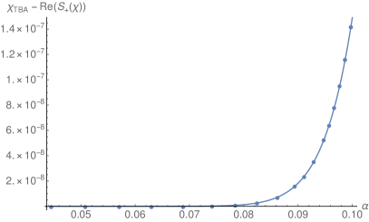
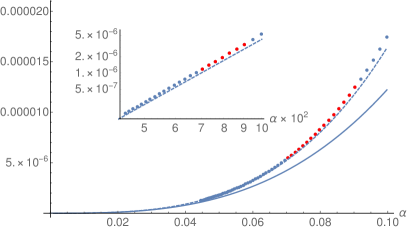
Figure 3: On the left hand side, one can see the difference between the TBA result and the real part of the lateral Borel resummation. The points show the numerics, while the solid line is nothing but the formula (3.14) truncated at $g_{3}$ in the expansion. The comparison of the so far unknown coefficients $g_{2}$ and $g_{3}$ in Table 1 to the subtracted numerical data $e^{2}/32e^{2/\alpha}\left(\chi_{\text{TBA}}-S_{+}(\chi)\right)-\left(2/\alpha+(3-\gamma_{E}-5\ln 2)+\ln\alpha+\alpha/2\right)$ is shown on the right. The points in red indicate the actual region over which the fit was performed (this was restricted, due to a substantial improvement in the error estimates of the coefficients). The continuous line is simply $\left(1/8-3\zeta_{3}/32\right)\alpha^{3}$, while the dashed line also contains the next term (the value of $g_{4}$ is numerical here): $g_{3}\alpha^{3}+g_{4}\alpha^{4}$. The inset shows the difference between the numerical data and the $g_{3}\alpha^{3}$ term on a log-log scale; the steepness of this line is consistent with the next term $g_{4}\alpha^{4}$ (dashed line). In order to maintain visibility we plotted only every fifth data point in the inset.

4 Disk capacitor problem

As explained in the introduction, we deal with the capacitance $C_{\text{phys}}$ of two oppositely charged, thin coaxial disks of radius $a$ at distance $d$ from each other. This quantity goes to

$$C_{\text{phys}}\to\epsilon_{0}\frac{\pi a^{2}}{d}$$ (4.1)

for $d\ll a$, i.e. to the well-known formula for parallel-plate capacitors; where $\epsilon_{0}$ is the vacuum permittivity. However, for finite $d$, the dependence on the distance is not so trivial. The problem can be solved exactly by Love’s equation (1949) Love:1949 (see a particularly simple derivation in Felderhof:2013 ):

$$f(x,\kappa)-\frac{\kappa}{\pi}\int_{-1}^{1}\mathrm{d}y\frac{f(y,\kappa)}{\kappa^{2}+(y-x)^{2}}=1,$$ (4.2)

where $\kappa\equiv d/a$, and the (dimensionless) capacitance can be expressed as an integral of the solution to this equation over the given domain:

$$C\equiv\frac{C_{\text{phys}}}{4\epsilon_{0}d},\qquad C=\frac{1}{2\kappa}\int_{-1}^{1}\mathrm{d}x\,f(x,\kappa).$$ (4.3)

Note that the integral equation above is nothing else, but the $\chi_{1}$ problem for the $O(3)$ kernel up to some identifications, and thus the capacitance is equivalent to the density $O_{11}$:

$$B\equiv\frac{\pi}{\kappa},\quad\chi_{1}(\theta)\equiv f(\kappa\,\theta/\pi,\kappa),\quad C\equiv O_{11}.$$ (4.4)

More recently, effective algorithms have been developed Marino:2019fuy ; Reichert:2020ymc for producing a large- and small-$\kappa$ expansion for the capacitance. The latter one is based on a modification of Volin’s method Volin:2010cq for the $r_{1}(\theta)=1$ source. The first nine coefficients of this expansion were given in Reichert:2020ymc analytically, however, to be able to perform an asymptotic analysis, one needs a lot more of them.

By using the relation (1.17) it is possible to reconstruct the perturbative coefficients of the capacitance from the particle- and energy-density of the $O(3)$ sigma model. As the running coupling proved to be handy for eliminating logarithms, we make use of it from the start. After using the relation among the derivatives (1.17) and the expressions for the corresponding $O_{cc}$ and $O_{1c}$ (2.24), (2.94) one gets

$$C^{\prime}(v)=-\frac{1}{8\pi v^{3}}\frac{\left[\hat{\rho}(v)-2v^{2}\hat{\rho}^{\prime}(v)\right]^{2}}{(1-v)W(v)-v^{2}W^{\prime}(v)},$$ (4.5)

where we also had to exchange the variables via $\partial_{B}=2v^{2}/(v-1)\partial_{v}$.

The above formula is exact, but we only used it to obtain the perturbative sector of the capacitance, which we denote by $C_{0}$. One has to integrate the series expansion of $C_{0}^{\prime}(v)$ formally term-by-term, and account for the loss of a constant term $c_{\mathrm{o}}=(L-L_{0})^{2}+2(L-L_{0})-1$ - we fixed this integration constant from the NNLO result derived first in wigglesworth1972comments ; chew1982microstrip . Here we introduced $L_{0}\equiv-\ln(8/e)$, just to show that for $L=L_{0}$ - which corresponds to the choice in (3.7) - some terms disappear. The expansion itself looks as:

$$C_{0}^{\prime}(v)=-\frac{1}{8\pi}\bigg{\{}v^{-3}+\left(L-L_{0}\right)v^{-2}-\left[\left(L-L_{0}\right)+\frac{1}{2}\left(L-L_{0}\right)^{2}+\frac{1}{4}-\frac{3}{4}\zeta_{3}\right]+\mathcal{O}(v)\bigg{\}}$$ (4.6)

and remarkably, the $1/v$ term is not present; thus there will be no $\ln(v)$ term in $C_{0}$:

$$C_{0}(v)=\frac{1}{16\pi}\bigg{\{} v^{-2}+2\left(L-L_{0}\right)v^{-1}+c_{\mathrm{o}}+$$

$$+\left[2\left(L-L_{0}\right)+\left(L-L_{0}\right)^{2}+\frac{1}{2}-\frac{3}{2}\zeta_{3}\right]v+\mathcal{O}(v^{2})\bigg{\}}$$ (4.7)

As a check, and to demonstrate its effectiveness, we may rewrite the same perturbative result shown in Reichert:2020ymc in terms of the special running coupling (3.7), leading to a formula, which is completely free of logarithms:

$$C_{0}(\beta)=\frac{1}{16\pi} \bigg{\{}\frac{1}{\beta^{2}}-1+\beta\left(\frac{1}{2}-\frac{3}{2}\zeta_{3}\right)+\beta^{2}\left(\frac{7}{6}-\frac{5}{2}\zeta_{3}\right)+\beta^{3}\left(\frac{1}{2}\zeta_{3}-\frac{135}{32}\zeta_{5}+\frac{11}{48}\right)+$$

$$+\beta^{4}\left(\frac{73}{8}\zeta_{3}+\frac{81}{16}\zeta_{3}^{2}-\frac{819}{32}\zeta_{5}-\frac{67}{120}\right)+$$

$$+\beta^{5}\left(\frac{25}{8}\zeta_{3}+\frac{705}{16}\zeta_{3}^{2}-\frac{1179}{32}\zeta_{5}-\frac{14175}{256}\zeta_{7}-\frac{23}{80}\right)+$$

$$+\beta^{6}\left(-\frac{4651}{192}\zeta_{3}+\frac{433}{4}\zeta_{3}^{2}+\frac{17919}{128}\zeta_{5}+\frac{27135}{128}\zeta_{3}\zeta_{5}-\frac{161109}{256}\zeta_{7}+\frac{9449}{20160}\right)+$$

$$+O(\beta^{7})\bigg{\}}.$$ (4.8)

Making use of the above method, we were able to “recycle” our 336 coefficients obtained for the $O(3)$ sigma model, and perform an asymptotic analysis for the perturbative coefficients of the capacitance. To be able to do this, we had to implement a slight modification (see Appendix D) of the original algorithm described in Appendix E.3 of Volin:2010cq . Otherwise, the numerical methods used in the asymptotic analysis, the lateral Borel resummation, and the exact solution of the TBA were very similar to the case of the $O(3)$ non-linear sigma model.

Let us then define the normalized quantity

$$\Phi(\beta)=16\pi\beta^{2}C_{0}(\beta)=\sum_{n=0}^{\infty}a_{n}\beta^{n}$$ (4.9)

whose expansion starts with $a_{0}=1$, then its asymptotics looks like

$$a_{n}=\frac{n!}{2^{n}}\left\{A_{0}+\frac{A_{1}}{n}+\frac{A_{2}}{n(n-1)}+\frac{A_{3}}{n(n-1)(n-2)}+\mathcal{O}(n^{-4})\right\}$$ (4.10)

where the leading coefficient is

$$A_{0}=-\frac{2^{6}}{\pi e^{4}},$$ (4.11)

and the asymptotic coefficients relative to this latter are:

$$\frac{A_{n}}{A_{0}}=1,\frac{7}{2},\frac{49}{8},\frac{149}{48}+6\zeta_{3},-\frac{6143}{384}+\frac{77}{2}\zeta_{3},\ldots.$$ (4.12)

As in Abbott:2020qnl ; Bajnok:2021zjm we found these results numerically, then searched for a plausible expression on the basis of odd zeta-s over the field of rationals. Similar to the $O(3)$ case, there were around 20 of these asymptotic coefficients, of which we could have a reliable numerical estimate. Then the ambiguity (the imaginary part of the lateral Borel resummation) looks as:

$$\mathrm{Im}\,S_{+}(\Phi)=-\frac{2^{7}}{e^{4}\beta}e^{-2/\beta}\left\{b_{0}+b_{1}\beta+b_{2}\beta^{2}+b_{3}\beta^{3}+\mathcal{O}(\beta^{4})\right\}$$ (4.13)

where the coefficients $b_{n}$ are in the following relation with the asymptotic ones:

$$b_{n}=\frac{A_{n}}{A_{0}}2^{-n},\quad b_{0}=1,\;b_{1}=\frac{7}{4},\;b_{2}=\frac{49}{32},\quad\ldots,$$ (4.14)

and we will show in the following, that eventually, this ambiguity seems to get canceled by the leading exponential imaginary term obtained from the Wiener-Hopf method: at least up to $b_{2}$, we could derive the same coefficients analytically.

To show this, we start again from the (1.11) relation for $O_{11}$, and notice immediately, that since the leading exponential term in $\chi_{1}(B)$ is of the order of $e^{-4B}$:

$$\dot{O}_{11}=\frac{1}{\pi}\chi_{1}^{2}(B),\quad\chi_{1}(B)=\frac{1}{2\sqrt{v}}\left(\hat{u}_{0}-ie^{-2}\hat{u}_{1}e^{-4B}+\mathcal{O}(e^{-8B})\right),$$ (4.15)

therefore the capacitance itself has a similar structure:

$$C=C_{0}+e^{-4B}C_{1}+\mathcal{O}(e^{-8B}),$$ (4.16)

and also that $C_{1}$ must be imaginary. By matching the $\mathcal{O}(1)$ parts, in terms of the running coupling (3.5) we can express $C_{0}$ as:

$$\frac{\mathrm{d}C_{0}}{\mathrm{d}v}=-\frac{1-v}{8\pi v^{3}}\hat{u}_{0}^{2},$$ (4.17)

and similarly, after matching the $e^{-4B}$ terms, one can reconstruct $C_{1}$ from:

$$C_{1}+\frac{v^{2}}{2(1-v)}\frac{\mathrm{d}C_{1}}{\mathrm{d}v}=\frac{i}{8\pi e^{2}v}\hat{u}_{0}\hat{u}_{1}.$$ (4.18)

We can calculate the perturbative part $\hat{u}_{0}$ by using the left equations of (3.3) and (3.4):

$$\hat{u}_{0}=1+\frac{1}{2}\beta+\frac{3}{8}\beta^{2}+\mathcal{O}(\beta^{3}).$$ (4.19)

Here, and throughout of this section, we use the special coupling (3.7). Finally, the non-perturbative part $\hat{u}_{1}$ is given by (B.48), (B.41), and (B.46). The necessary input is just the above expansion coefficients $r_{1}=\frac{1}{2},\;r_{2}=\frac{3}{8}$ of $\hat{u}_{0}$ from (4.19), and $\Omega_{1}=\frac{13}{32}$ from the expansion of $w_{0}$ (2.73). Then up to the same order in $\beta$:

$$\hat{u}_{1}=1+\frac{3}{4}\beta+\frac{9}{32}\beta^{2}+\mathcal{O}(\beta^{3}).$$ (4.20)

Thus the reconstructed $C_{1}$ is

$$C_{1}=\frac{i}{8\pi e^{2}\beta}\left\{1+\frac{7}{4}\beta+\frac{49}{32}\beta^{2}+\mathcal{O}(\beta^{3})\right\},$$ (4.21)

and as one can see the coefficients here match those in (4.14). Let us note that calculating one further coefficient still seems to be feasible by the methods described in this paper.

The above findings support the claim, that the method originally developed in Marino:2021dzn and reformulated in this paper provides us the physical value of the given quantity since here we saw that the lateral Borel resummation of the perturbative part - which we got by expanding the integrals over the contour $\mathcal{C}_{+}$ in (2.34) - together with the explicit residue terms is at least free of the leading ambiguity. Let us emphasize that this fact - and the one that for the capacitance resurgence seems to explain also the leading real exponential contribution in the trans-series (see later) - supports the strong version of resurgence theory, namely that the perturbative coefficients contain all information about the trans-series expansion. This is in contrast to the $O(3)$ sigma model’s energy density, where parts of the trans-series are missed by the median resummation.

To complete the numerical analysis, we compared the lateral Borel resummation above the imaginary axis to a high-precision numerical solution of the integral equation as for the $O(3)$ case:

$$\Phi_{\mathrm{TBA}}-\mathrm{Re}\,S_{+}(\Phi)=-\frac{2^{12}}{e^{8}\beta^{3}}e^{-4/\beta}\left\{c_{0}+c_{1}\beta+c_{2}\beta^{2}+c_{3}\beta^{3}+\mathcal{O}(\beta^{4})\right\}$$ (4.22)

where the $c_{n}$ coefficients are measured to be those shown in Table 2.

exact value	numerical estimate
$c_{0}=1$	$\;\;\;\;\;\;\;\;\;\;0.99999999(8\!\pm\!4)$
$c_{1}=\frac{3}{2}$	$\;\;\;\;\;\;\;\;\;\;1.500000000(4\!\pm\!8)$
$c_{2}=\frac{5}{4}$	$\;\;\;\;\;\;\;\;\;\;1.2499999(93\!\pm\!16)$
$c_{3}\overset{?}{=}\frac{3}{4}\zeta_{3}+\frac{67}{96}=1.59945934\ldots$	$\;\;\;\;\;\;\;\;\;\;1.599459(29\!\pm\!12)$
$c_{4}=?$	$\;\;\;\;\;\;\;\;\;\;2.819320(4\!\pm\!6)$
$c_{5}=?$	$\;\;\;\;\;\;\;\;\;\;6.571694\pm 0.000021$

Table 2: The coefficients of the exponentially suppressed discrepancy between the TBA numerics and the real part of the lateral Borel resummation. The agreement of the recognized coefficients to the numerical data can be seen in Figure 4. Note that the exact value of $c_{3}$ is only an educated guess.

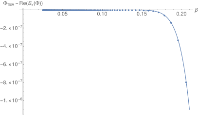
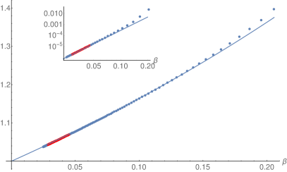
Figure 4: On the left, the points show the numerics, that is, the l.h.s of (4.22), while the solid line is nothing but the formula on the r.h.s. up to $c_{3}$ in the expansion. On the right, the comparison of the same coefficients in Table 2 to the numerical data $-e^{8}\beta^{3}/2^{12}e^{4/\beta}\left(\Phi_{\text{TBA}}-S_{+}(\Phi)\right)$ is shown. The red points show the fitting region again. The continuous line is the exact polynomial $1+3/2\beta+5/4\beta^{2}+(3/4\zeta_{3}+67/96)\beta^{3}$. The inset shows the difference between the numerical data and the above third-order polynomial on a log-log scale; its steepness is consistent with the next term being proportional to $\beta^{4}$ in the expansion.

The number of perturbative coefficients was not sufficient enough to obtain a reliable estimate of the second alien derivative of $\Phi(\beta)$ at the closest singularity on its Borel plane, which is assumed to be proportional to the above difference (4.22). Thus, here we only try to support the leading asymptotic coefficient by resurgence theory. That is, we expect the asymptotic structure of the $A_{n}$-s themselves in (4.10) to look like:

$$\frac{A_{n-1}}{A_{0}}=n!\left\{\mathcal{A}_{0}+\frac{\mathcal{A}_{1}}{n}+\frac{\mathcal{A}_{2}}{n(n-1)}+\frac{\mathcal{A}_{3}}{n(n-1)(n-2)}+\mathcal{O}(n^{-4})\right\},$$ (4.23)

where the numerical estimate for the leading asymptotic coefficient is consistent with $\mathcal{A}_{0}=\frac{16}{e^{4}\pi}$ up to two digits.

We tested this number as follows. The median resummation formula Abbott:2020qnl is

$$S_{\mathrm{med}}(\Phi)-\mathrm{Re}\,S_{+}(\Phi)=-\frac{e^{-4/\beta}}{8}S_{+}(D_{2}^{2}\Phi+D_{1}D_{3}\Phi)+\mathcal{O}(e^{-6/\beta}),$$ (4.24)

where $D_{n}\Phi$ is the alien derivative at $s=n$ on the Borel plane corresponding to the asymptotic series (4.9) and its Borel transform

$$B(\Phi)=\sum_{n=0}^{\infty}\frac{a_{n}}{n!}s^{n}.$$ (4.25)

If we assume that $D_{1}D_{3}\Phi=0$, as we did for the $O(4)$ case Abbott:2020qnl , then the strength of the (4.24) difference is governed by the second alien derivative $D_{2}^{2}\Phi$ only. After substituting the asymptotics (4.10) and (4.23), the structure of the function $B(\Phi)$ looks as:

$$B(\Phi) =\text{ non-singular }+\frac{A_{0}}{1-s/2}-\ln\left(1-\frac{s}{2}\right)\bigg{\{}\text{ non-singular }+$$

$$+A_{0}\left[-\frac{2^{4}\,\mathcal{A}_{0}}{(s-4)^{3}}+\frac{2^{2}\,\mathcal{A}_{1}}{(s-4)^{2}}-\frac{2\,\mathcal{A}_{2}}{s-4}-\left(\mathcal{A}_{3}+\mathcal{O}(s-4)\right)\ln(2-s/2)\right]\bigg{\}},$$ (4.26)

and thus the leading contribution in $D^{2}_{2}\Phi$ comes from the $1/(s-4)^{3}$ term multiplying the logarithmic cut. The leading term in the second alien derivative can be calculated as

$$S_{+}(D^{2}_{2}\Phi) =S_{+}(D_{2}\Phi)-S_{-}(D_{2}\Phi)=$$

$$=2^{4}A_{0}\mathcal{A}_{0}\times\frac{1}{\beta}\int_{\mathcal{H}}\mathrm{d}s\,e^{-s/\beta}\ln\left(1-\frac{s}{2}\right)\left(\frac{1}{(s-4)^{3}}+\mathcal{O}\left((s-4)^{-2}\right)\right)=$$

$$=2^{4}A_{0}\mathcal{A}_{0}\times\frac{(-2\pi i)^{2}}{\beta}\times e^{-4/\beta}\left(\frac{1}{2\beta^{2}}+\mathcal{O}\left(\beta^{-1}\right)\right),$$ (4.27)

where one $(-2\pi i)$ factor comes from the discontinuity of the logarithm, and another comes by Cauchy theorem when evaluating the Hankel-type contour $\mathcal{H}$ around the logarithmic cut. This way (4.24) and (4.22) are consistent with each other, at least up to the Stokes constant - the strength of the term - before the exponential:

$$S_{\mathrm{med}}(\Phi)-\mathrm{Re}\,S_{+}(\Phi)=-\frac{e^{-4/\beta}}{8\beta^{3}}\times\left(-\pi^{2}2^{5}A_{0}\mathcal{A}_{0}\right)=-\frac{2^{12}}{e^{8}\beta^{3}}e^{-4/\beta}.$$ (4.28)

Finally, we give the capacitance formula in terms of the original variable $\kappa$, which is proportional to the distance of the plates:

$$\mathcal{C} =S_{+}\left(\frac{1}{4\kappa}+\frac{\mathsf{L}-1}{4\pi}+\frac{\kappa}{16\pi^{2}}\left(\mathsf{L}^{2}-2\right)+\mathcal{O}(\kappa^{2})\right)$$

$$+\frac{i}{e^{2}}e^{-4\pi/\kappa}S_{+}\left\{\frac{1}{2\kappa}+\frac{8\mathsf{L}-1}{16\pi}+\frac{\kappa(8\mathsf{L}(4\mathsf{L}+7)-39)}{256\pi^{2}}+\mathcal{O}(\kappa^{2})\right\}+\mathcal{O}(e^{-8\pi/\kappa}),$$ (4.29)

where $\mathsf{L}\equiv\ln\left(16\pi/\kappa\right)$, and $\mathcal{C}\equiv\kappa/\pi\,C$ is another possible definition of the dimensionless capacitance used in the introduction and in Reichert:2020ymc . The difference between the real part of the lateral Borel resummation $S_{+}(\mathcal{C})$, and the TBA data looks now as:

$$\mathcal{C}_{\mathrm{TBA}}-\mathrm{Re}\,S_{+}(\mathcal{C})=-\frac{1}{e^{4}}e^{-8\pi/\kappa}\left\{\frac{1}{4\kappa}+\frac{4\mathsf{L}-1}{16\pi}+\frac{\kappa\left(4\mathsf{L}^{2}+6\mathsf{L}-5\right)}{64\pi^{2}}+\mathcal{O}(\kappa^{2})\right\}.$$ (4.30)

5 Conclusion

In this paper we investigated integral equations with kernels related to the $O(N)$ sigma models. We analyzed various observables including the density $O_{c1}$ and energy density $O_{cc}$ of the groundstate energy of the $O(N)$ sigma models in a magnetic field and the capacitance of the circular plate capacitor $O_{11}$. We also established relations between these observables, see (1.17). We advanced in the systematic, Wiener-Hopf type solution of this class of models considerably. We first simplified the Wiener-Hopf equations to ensure that only one integral operator appears. Based on the analytical structure of its kernel we could introduce a running coupling and show that all observables can be expanded solely in its powers without any logarithms of it. We also formulated a form of the equations which handled the non-perturbative terms systematically showing also only power-like dependence on the running coupling. These simplified equations are easier to handle than their previous versions and we also developed a method based on Laplace transformation how the various orders could be calculated explicitly. Combining the relations between the observables and the already known perturbative expansions we could advance in the calculations of new non-perturbative terms. We investigated the structure of the non-perturbative corrections and determined their leading terms.

As the $O(3)$ kernel is exceptional, we elaborated on this case separately. We studied the behaviour of the free energy in the $O(3)$ sigma model, where we compared the exactly determined non-perturbative terms to the direct numerical solution of the integral equations and found complete agreement. We also confronted the asymptotics of the perturbative series with the leading non-perturbative corrections and confirmed the previous findings that they do not match.

The introduction of our running coupling simplified the perturbative expansion of the coaxial disk capacitance drastically. By expressing its derivatives in terms of the density and groundstate energy of the $O(3)$ sigma model we were able to analyze also its leading non-perturbative corrections. We then investigated how resurgence theory works and we found that the asymptotics of the perturbative expansion contained all information about the non-perturbative terms. We checked these results against the numerical solution of the integral equation.

Our simplified equations can be used to calculate the trans-series representation of the various observables. This trans-series is a sum of all the exponentially suppressed terms $\nu^{n}$ with $\nu=e^{-1/v-L}/v$ multiplied by a typically asymptotic series in the running coupling $v$. We indicate in Table 3 the structure of the non-perturbative corrections for various observables in the $O(N)$ model. The terms in red are not connected to the asymptotics of the perturbative series, while the ones in black are. The anomalous (constant) term in the energy density for the $O(N)$ sigma models for $N\geq 5$ can be attributed to the different definitions of the zero point energy in the two descriptions: in perturbation theory the groundstate energy vanishes for zero magnetic field, $h=0$, while in the TBA formulation it vanishes at $h=m$ Marino:2021dzn . The biggest difference is in the $O(3)$ model, where the real part of the leading non-perturbative corrections is not related to the asymptotic perturbative series. We attributed this behaviour to the presence of instantons Bajnok:2021zjm , and this has been verified in Marino:2022ykm . This makes the $O(3)$ theory exceptional among the other $O(N)$ models. Other non-perturbative corrections, which are related to the asymptotics of the perturbative series were previously connected to renormalons DiPietro:2021yxb ; Marino:2021six .

	$O_{cc}$	${\color[rgb]{1,0,0}\nu}$	$\nu^{2}$	${\color[rgb]{1,0,0}\nu^{3}}$	$\nu^{4}$	${\color[rgb]{1,0,0}\nu}^{{\color[rgb]{1,0,0}5}}$	$\nu^{6}$			$\nu^{l}$
$O(3)$	$O_{c1}$	${\color[rgb]{1,0,0}\nu}$	$\nu^{2}$	${\color[rgb]{1,0,0}\nu^{3}}$	$\nu^{4}$	${\color[rgb]{1,0,0}\nu^{5}}$	$\nu^{6}$			$\nu^{l}$
	$O_{11}$		$\nu^{2}$		$\nu^{4}$		$\nu^{6}$			$\nu^{2l}$
$O(4)$	$O_{cc}$	$\nu$	$\nu^{2}$		$\nu^{4}$		$\nu^{6}$			$\nu^{2l}$
	$O_{c1}$		$\nu^{2}$		$\nu^{4}$		$\nu^{6}$			$\nu^{2l}$
$O(5)$	$O_{cc}$	${\color[rgb]{1,0,0}\nu}$					$\nu^{6}$			$\nu^{6l}$
	$O_{c1}$						$\nu^{6}$			$\nu^{6l}$
$O(6)$	$O_{cc}$	${\color[rgb]{1,0,0}\nu}$			$\nu^{4}$					$\nu^{4l}$
	$O_{c1}$				$\nu^{4}$					$\nu^{4l}$
$O(2k)$	$O_{cc}$	${\color[rgb]{1,0,0}\nu}$						$\nu^{2(k-1)}$		$\nu^{2l(k-1)}$
	$O_{c1}$							$\nu^{2(k-1)}$		$\nu^{2l(k-1)}$
$O(2k+1)$	$O_{cc}$	${\color[rgb]{1,0,0}\nu}$						$\nu^{2(2k-1)}$		$\nu^{2l(2k-1)}$
	$O_{c1}$							$\nu^{2(2k-1)}$		$\nu^{2l(2k-1)}$

Table 3: Structure of the exponential corrections in $\nu=e^{-2B}$ for different $O(N)$ models and observables. The non-perturbative terms in red are not completely related to the asymptotics of the perturbative series, although for $N\geq 5$ this mismatch can be attributed to the different definitions of the $h=0$ bulk energy constant.

Our formulation allows a systematic calculation of the non-perturbative terms. Beyond the leading order, however, several contributions will appear to each trans-series term and a future analysis should work out their details. Also it would be important to understand that to which resummation prescription, median or not, our method will lead to. The technique based on the Laplace transformation gives explicit expressions to the various perturbative coefficients, but becomes more and more complicated at higher orders. It would be very nice to adapt Volin’s method beyond the perturbative order and calculate non-perturbative corrections in a similar fashion. In the $O(4)$ model we observed very interesting relations between different trans-series terms Abbott:2020mba ; Abbott:2020qnl ; Bajnok:2021dri . It would be very insightful to derive those relations directly from the integral equations, or derive similar relations for other trans-series terms. The introduction of the running coupling simplified all our calculations considerably. We believe they should also play a central role in other asymptotically free models, too.

Appendix A Building blocks needed for the Wiener-Hopf analysis

In this appendix we collect a number of definitions, results and technical tools which are used in the main text.

The Fourier transform of the kernel $K(\theta)$ is

$$\tilde{K}(\omega)=\int_{-\infty}^{\infty}d\theta e^{i\omega\theta}K(\theta)=\frac{e^{-\pi|\omega|}+e^{-2\pi\Delta|\omega|}}{1+e^{-\pi|\omega|}}.$$ (A.1)

We will define the Fourier transform of other functions analogously and also indicate it by a tilde. Note that for $O(3)$ the Fourier transform of the kernel simplifies to $e^{-\pi|\omega|}$.

In the Wiener-Hopf analysis an important role is played by the multiplicative decomposition

$$G_{+}(\omega)G_{-}(\omega)=\frac{1}{1-\tilde{K}(\omega)},$$ (A.2)

where $G_{\pm}$ are analytic in $H_{\pm}$, the upper and lower complex half-planes, respectively. Note that $\tilde{K}(0)=1$ and $G_{\pm}(\omega)$ are singular near $\omega=0$ like $|\omega|^{-1/2}$. This is the typical behaviour for bosonic models. (For fermionic models $G_{\pm}$ are regular at $\omega=0$ and this makes their Wiener-Hopf analysis simpler.) $\tilde{K}(\omega)$ is real and symmetric and therefore

$$G_{-}(\omega)=G_{+}(-\omega).$$ (A.3)

$G_{+}$ is given explicitly by

$$G_{+}(\omega)=\frac{1}{\sqrt{-i\Delta\omega}}\ \frac{\Gamma(1-i\omega\Delta)}{\Gamma(1/2-i\omega/2)}\exp\left\{-i\omega\Delta[1-\ln(-i\omega\Delta)]+i\omega[1-\ln(-i\omega/2)]/2\right\}.$$ (A.4)

For small real $\omega$

$$G_{+}(\omega)\approx\frac{1}{\sqrt{\pi\Delta|\omega|}}e^{\frac{i\pi}{4}{\rm sign}(\omega)}$$ (A.5)

and for asymptotically large argument in $H_{+}$

$$G_{+}(i\kappa)=1+O(1/\kappa),\qquad\quad\kappa\to\infty.$$ (A.6)

We also need

$$G_{+}(i)=\frac{1}{\sqrt{2\Delta}}\Gamma(1+\Delta)e^{\gamma_{1}/2-\Delta\ln\Delta},\qquad\quad\gamma_{1}=2\Delta-1.$$ (A.7)

Functions $f(\omega)$ vanishing for $|\omega|\to\infty$ can be decomposed additively into $f^{(+)}$ and $f^{(-)}$, analytic in $H_{+}$ and $H_{-}$, respectively:

$$f^{(\pm)}(\omega)=\mp\frac{1}{2\pi i}\int_{-\infty}^{\infty}\frac{f(\omega^{\prime})d\omega^{\prime}}{\omega-\omega^{\prime}}.$$ (A.8)

For real $\omega$, $f^{(+)}(\omega)+f^{(-)}(\omega)=f(\omega)$. If $f(\omega)$ is already analytic in $H_{+}$ and vanishes for large $|\omega|$ then $f^{(+)}(\omega)=f(\omega)$ and $f^{(-)}(\omega)=0$, and analogously for $f(\omega)$ analytic in $H_{-}$.

$G_{+}$ is analytic in $H_{+}$ by definition but it is also analytic in $H_{-}$, except for the negative imaginary axis (where it is discontinuous and also has poles). Similarly $G_{-}$ is everywhere analytic, except along the positive imaginary axis. An important variable in our analysis is

$$\alpha(\omega)=e^{2i\omega B}\frac{G_{-}(\omega)}{G_{+}(\omega)},$$ (A.9)

which is discontinuous along the positive imaginary axis and has poles there. Explicitly, just on the left and right side of the imaginary axis,

$$\alpha(2i\xi\pm\varepsilon)=e^{-4B\xi}[\mp i\cos(\pi\gamma_{1}\xi)+\sin(\pi\gamma_{1}\xi)]H(\xi),$$ (A.10)

where

$$H(\xi)=e^{2\gamma_{1}\xi\ln 2\xi}H_{p}(\xi),$$ (A.11)

with

$$H_{p}(\xi)=\frac{\Gamma(1-2\Delta\xi)}{\Gamma(1+2\Delta\xi)}\,\frac{\Gamma(1/2+\xi)}{\Gamma(1/2-\xi)}\,e^{2\xi[2\Delta\ln\Delta+\ln 2-\gamma_{1}]}.$$ (A.12)

An important property of $H_{p}(\xi)$ is that it can be expanded around $\xi=0$ in powers of $\xi$:

$$H_{p}(\xi)=1+2\alpha_{1}\xi+O(\xi^{2}),$$ (A.13)

where

$$\alpha_{1}=\gamma_{1}(\gamma_{E}-1+\ln\Delta)+\ln(\Delta/2).$$ (A.14)

The discontinuity is

$$\alpha(2i\xi+\varepsilon)-\alpha(2i\xi-\varepsilon)=-2ie^{-4B\xi}\beta(\xi),\qquad\quad\beta(\xi)=\cos(\pi\gamma_{1}\xi)\,H(\xi).$$ (A.15)

$H(\xi)$ is meromorphic in $H_{+}$, it has poles (and zeroes) on the positive imaginary axis. The poles are located at

$$\xi=\xi_{\ell}=\ell\xi_{o},\qquad\ell=1,2,\dots\qquad\xi_{o}=\left\{\begin{matrix}\frac{N-2}{2}\qquad\quad&N\ {\rm even,}\\ N-2\qquad\quad&N\ {\rm odd.}\end{matrix}\right.$$ (A.16)

The zeroes are at

$$\xi=m+\frac{1}{2},\qquad\quad m=0,1,2\dots$$ (A.17)

with the exception (for odd $N$) of $m$ integers of the form

$$m=\frac{N-3}{2}+(N-2)k,\qquad\quad k=0,1,2\dots$$ (A.18)

We see that

$$H(1/2)=0,\qquad\quad{\rm except\ for\ }N=3.$$ (A.19)

We also see that

$$\sin(\pi\gamma_{1}\xi_{\ell})=0,\qquad\quad\cos(\pi\gamma_{1}\xi_{\ell})=\varepsilon_{\ell}$$ (A.20)

where

$$\varepsilon_{\ell}=\left\{\begin{matrix}(-1)^{\ell}\qquad\quad&N\ {\rm odd,}\\ (-1)^{N\ell/2}\qquad\quad&N\ {\rm even.}\end{matrix}\right.$$ (A.21)

Near $\xi=\xi_{\ell}$ if

$$H(\xi)\approx\frac{\tilde{H}_{\ell}}{\xi-\xi_{\ell}}$$ (A.22)

with some residue $\tilde{H}_{\ell}$ then

$$\alpha(2i\xi\pm\varepsilon)=\mp ie^{-4B\xi_{\ell}}\,\frac{H_{\ell}}{\xi-\xi_{\ell}},\qquad\quad\beta(\xi)\approx\frac{H_{\ell}}{\xi-\xi_{\ell}},\qquad\quad H_{\ell}=\varepsilon_{\ell}\tilde{H}_{\ell}.$$ (A.23)

We will also need the behaviour of $\alpha(2i\xi\pm\varepsilon)$ and $\beta(\xi)$ near $\xi=1/2$. We find

$$\alpha(2i\xi\pm\varepsilon)=e^{-2B}\left\{h_{o}+h_{1}^{\pm}(\xi-1/2)+O((\xi-1/2)^{2})\right\},$$ (A.24)

where

$$h_{o}=\frac{\delta_{N,3}}{e},\qquad\quad h_{1}^{\pm}=\left\{\begin{matrix}\left(\mp i\cos\frac{\pi\gamma_{1}}{2}+\sin\frac{\pi\gamma_{1}}{2}\right)\tilde{h}_{1}\qquad\quad&N\geq 4,\\ \tilde{h}_{1}-\frac{4B}{e}\pm\frac{i\pi}{e}\qquad\qquad&N=3,\end{matrix}\right.$$ (A.25)

and

$$\tilde{h}_{1}=\left\{\begin{matrix}-\frac{\Gamma(1-\Delta)}{\Gamma(1+\Delta)}\exp\{2\Delta\ln\Delta+\ln 2-\gamma_{1}\}\qquad\quad&N\geq 4,\\ \frac{2}{e}(\gamma_{E}-1+\ln 2)\qquad\quad&N=3.\end{matrix}\right.$$ (A.26)

Again, we see that $\alpha(i)=0$, except for $N=3$. On the other hand, $\beta(1/2)$ always vanishes:

$$\beta(\xi)=\beta_{o}(\xi-1/2)+O((\xi-1/2)^{2}),$$ (A.27)

where

$$\beta_{o}=\left\{\begin{matrix}\cos\left(\frac{\pi\gamma_{1}}{2}\right)\tilde{h}_{1}\qquad\quad&N\geq 4,\\ -\pi/e\qquad\quad&N=3.\end{matrix}\right.$$ (A.28)

Appendix B The $\chi_{1}$ problem

The source term here is

$$r_{1+}(\omega)=\frac{e^{2i\omega B}}{i\omega}-\frac{1}{i\omega}.$$ (B.1)

We proceed analogously to the $\chi_{c}$ problem and absorb the first term into the new unknown

$$\hat{Q}_{+}(\omega)=Q_{+}(\omega)+\frac{G_{+}(\omega)}{i\omega}.$$ (B.2)

Again, the rest of the source term can be easily dealt with by closing the contour of integration in $H_{-}$.

However, there is an extra difficulty in this problem since the new variable (B.2) has a non-integrable singularity at the origin:

$$\hat{Q}_{+}(2i\xi)\approx\frac{-1}{2\xi\sqrt{2\xi\pi\Delta}}.$$ (B.3)

This means that we have to be careful with the derivation and regularize integrals around the origin. This regularization can be removed at the end of the calculation after applying appropriate subtractions to the integrals. We again deform the original contour to the (regularized) ${\cal C}_{LR}$ contour and formulate the integral equation in terms of principal value integration. No terms proportional to $e^{-2B}$ arise here and finally we arrive at

$$\begin{split}\xi\hat{Q}_{+}&(2i\xi)-\frac{1}{\pi}{\cal P}\int_{0}^{\infty}\frac{e^{-4B\xi^{\prime}}\beta(\xi^{\prime})\xi^{\prime}\hat{Q}_{+}(2i\xi^{\prime})}{\xi+\xi^{\prime}}d\xi^{\prime}\\ &+\frac{1}{\pi}{\cal P}\int_{0}^{\infty}\Big{\{}e^{-4B\xi^{\prime}}\beta(\xi^{\prime})\hat{Q}_{+}(2i\xi^{\prime})+\frac{1}{2\xi^{\prime}\sqrt{2\xi^{\prime}\pi\Delta}}\Big{\}}d\xi^{\prime}=0.\end{split}$$ (B.4)

We simplify the equation by introducing the rescaled variable

$$K(x)=\sqrt{v\pi\Delta}vx\hat{Q}_{+}(ivx)$$ (B.5)

and rewrite the integrals to go along the contour ${\cal C}_{+}$ (plus residue terms):

$$\begin{split}K(x)-&\frac{1}{\pi}\int_{{\cal C}_{+}}\frac{e^{-y}{\cal A}(y)K(y)}{x+y}dy+\frac{ivx}{\xi_{o}}\sum_{\ell=1}^{\infty}\frac{H_{\ell}y_{\ell}}{\ell(2\ell\xi_{o}+vx)}\nu^{2\ell\xi_{o}}\\ +&\frac{1}{\pi}\int_{{\cal C}_{+}}\Bigg{\{}e^{-y}{\cal A}(y)\frac{K(y)}{y}+\frac{1}{y\sqrt{y}}\Bigg{\}}dy=0.\end{split}$$ (B.6)

Here

$$y_{s}=\sqrt{v\pi\Delta}2s\xi_{o}\hat{Q}_{+}(2is\xi_{o})$$ (B.7)

and it can be calculated from

$$\begin{split}y_{s}-&\frac{v}{\pi}\int_{{\cal C}_{+}}\frac{e^{-x}{\cal A}(x)K(x)}{2s\xi_{o}+vx}dx+\frac{is}{\xi_{o}}\sum_{\ell=1}^{\infty}\frac{H_{\ell}y_{\ell}}{\ell(s+\ell)}\nu^{2\ell\xi_{o}}\\ +&\frac{1}{\pi}\int_{{\cal C}_{+}}\Bigg{\{}e^{-x}{\cal A}(x)\frac{K(x)}{x}+\frac{1}{x\sqrt{x}}\Bigg{\}}dx=0.\end{split}$$ (B.8)

We again represent our variables as the trans-series

$$K(x)=\sum_{m=0}^{\infty}K_{m}(x)\,\nu^{2m\xi_{o}},\qquad\quad y_{s}=\sum_{m=0}^{\infty}y_{s,m}\,\nu^{2m\xi_{o}}.$$ (B.9)

Note that these are valid for both the $N\geq 4$ and the $N=3$ cases. The LO and NLO equations are

$$K_{0}(x)-\frac{1}{\pi}\int_{{\cal C}_{+}}\frac{e^{-y}{\cal A}(y)K_{0}(y)}{x+y}dy+\frac{1}{\pi}\int_{{\cal C}_{+}}\Bigg{\{}e^{-y}{\cal A}(y)\frac{K_{0}(y)}{y}+\frac{1}{y\sqrt{y}}\Bigg{\}}dy=0,$$ (B.10)

$$\overline{K}_{1}(x)+\frac{1}{\pi}\int_{{\cal C}_{+}}\frac{e^{-y}{\cal A}(y)\overline{K}_{1}(y)}{x+y}dy=-\frac{iv}{\xi_{o}}\,\frac{H_{1}y_{1,0}}{2\xi_{o}+vx}.$$ (B.11)

Here

$$\overline{K}_{1}(x)=\frac{K_{1}(x)}{x}$$ (B.12)

and

$$y_{1,0}=\frac{v}{\pi}\int_{{\cal C}_{+}}\frac{e^{-y}{\cal A}(y)K_{0}(y)}{2\xi_{o}+vy}dy-\frac{1}{\pi}\int_{{\cal C}_{+}}\Bigg{\{}e^{-y}{\cal A}(y)\frac{K_{0}(y)}{y}+\frac{1}{y\sqrt{y}}\Bigg{\}}dy.$$ (B.13)

For the perturbative expansion of the leading coefficient we will use

$${\cal A}(x)K_{0}(x)=\omega(x)=\sum_{k=0}^{\infty}v^{k}\omega_{k}(x)$$ (B.14)

and also define the ($B$-independent) functions $g_{k}$ by

$$\omega_{k}(x)=xg_{k}(x)-\frac{\delta_{k,0}}{\sqrt{x}}.$$ (B.15)

Later we will need their moments

$$\bar{\gamma}_{k,r}=\frac{1}{\pi}\int_{0}^{\infty}e^{-x}x^{r}g_{k}(x)dx,\qquad\quad\bar{\gamma}_{k}=\bar{\gamma}_{k,0}$$ (B.16)

and we will also need

$$I(p)=\int_{0}^{\infty}\frac{e^{-px}-1}{x\sqrt{x}}dx=-2\sqrt{\pi p},\qquad\quad I^{(r)}(p)=\frac{d^{r}}{dp^{r}}\,I(p).$$ (B.17)

The first two components satisfy

$$g_{0}(x)+\frac{1}{\pi}\int_{0}^{\infty}\frac{e^{-y}g_{0}(y)}{x+y}dy=\frac{1}{\pi}\int_{0}^{\infty}\frac{e^{-y}-1}{(x+y)y\sqrt{y}}dy,$$ (B.18)

$$g_{1}(x)+\frac{1}{\pi}\int_{0}^{\infty}\frac{e^{-y}g_{1}(y)}{x+y}dy=\left(xg_{0}(x)-\frac{1}{\sqrt{x}}\right)L_{1}(\ln x).$$ (B.19)

These two integral equations are solved explicitly in appendix C.

The calculation of the density integral and the boundary value of $\chi_{1}$ is analogous to the derivation of (B.4). After a long calculation we get

$$O_{1c}=\frac{e^{B}G_{+}(i)}{2\pi}\left\{\frac{\delta_{N,3}}{e}\,\hat{Q}_{+}(i)\,\nu+\frac{2}{\pi}{\cal P}\int_{0}^{\infty}\frac{d\xi}{1-2\xi}\left[e^{-4B\xi}\beta(\xi)\hat{Q}_{+}(2i\xi)+\frac{1}{2\xi\sqrt{2\xi\pi\Delta}}\right]\right\}$$ (B.20)

and

$$\chi_{1}(B)=\frac{2}{\pi}{\cal P}\int_{0}^{\infty}\left\{e^{-4B\xi}\beta(\xi)\hat{Q}_{+}(2i\xi)+\frac{1}{2\xi\sqrt{2\xi\pi\Delta}}\right\}d\xi.$$ (B.21)

For $N=3$ the trans-series for the density $O_{1c}$ contains all powers of $\nu$. For $\chi_{1}(B)$, however, the trans-series is of the form

$$\chi_{1}(B)=\frac{1}{\sqrt{v\pi\Delta}}\sum_{m=0}^{\infty}u_{m}\,\nu^{2m\xi_{o}}$$ (B.22)

for all $N$. The first two coefficients are

$$u_{0}=\frac{1}{\pi}\int_{{\cal C}_{+}}\left\{e^{-x}{\cal A}(x)\frac{K_{0}(x)}{x}+\frac{1}{x\sqrt{x}}\right\}dx=\frac{1}{\pi}\int_{{\cal C}_{+}}\left\{e^{-x}\frac{\omega(x)}{x}+\frac{1}{x\sqrt{x}}\right\}dx,$$ (B.23)

$$u_{1}=\frac{1}{\pi}\int_{{\cal C}_{+}}e^{-x}{\cal A}(x)\overline{K}_{1}(x)dx+\frac{i}{\xi_{o}}H_{1}y_{1,0}.$$ (B.24)

We now expand $u_{0}$ perturbatively:

$$u_{0}=\sum_{k=0}^{\infty}v^{k}u_{0,k}.$$ (B.25)

Here

$$u_{0,0}=\frac{1}{\pi}\int_{0}^{\infty}dx\left[e^{-x}g_{0}(x)+\frac{1}{x\sqrt{x}}\left(1-e^{-x}\right)\right]=\bar{\gamma}_{0}+\frac{2}{\sqrt{\pi}},$$ (B.26)

$$u_{0,k}=\bar{\gamma}_{k},\qquad k=1,2,\dots$$ (B.27)

In appendix C we calculate

$$\bar{\gamma}_{0}=\frac{\sqrt{\pi}}{2}-\frac{2}{\sqrt{\pi}}$$ (B.28)

and so we can write the perturbative expansion of $u_{0}$ as

$$u_{0}=\frac{\sqrt{\pi}}{2}\left(1+\sum_{k=1}^{\infty}v^{k}r_{k}\right),\qquad\quad r_{k}=\frac{2}{\sqrt{\pi}}\bar{\gamma}_{k}.$$ (B.29)

The NLO coefficient $r_{1}$ is calculated in appendix C:

$$r_{1}=r_{o}+\frac{L}{2}.$$ (B.30)

Next we turn to $O_{1c}$. We start with the trans-series expansion of

$$\hat{Q}_{+}(i)=\frac{1}{\sqrt{v\pi\Delta}}K(1/v)=\frac{1}{\sqrt{v\pi\Delta}}\sum_{m=0}^{\infty}\hat{Q}_{+,m}\,\nu^{2m\xi_{o}}$$ (B.31)

and consider the leading coefficient

$$\begin{split}\hat{Q}_{+,0}&=\frac{v}{\pi}\int_{{\cal C}_{+}}\frac{e^{-x}\omega(x)}{1+vx}dx-\frac{1}{\pi}\int_{{\cal C}_{+}}\left[\frac{e^{-x}\omega(x)}{x}+\frac{1}{x\sqrt{x}}\right]dx\\ &=-\frac{\sqrt{\pi}}{2}\Bigg{\{}1+\frac{2}{\sqrt{\pi}}\Big{[}\sum_{p+q\not=0}v^{p+q}(-1)^{q}\bar{\gamma}_{p,q}-\frac{1}{\pi}\sum_{q=1}^{\infty}v^{q}\,I^{(q)}(1)\Big{]}\Bigg{\}}.\end{split}$$ (B.32)

Alternatively, $\hat{Q}_{+}(i)$ can be written as

$$\hat{Q}_{+}(i)=-\frac{1}{2\sqrt{v\Delta}}\left\{1+\sum_{k=1}^{\infty}\tilde{R}_{k}v^{k}\right\}+O(\nu^{2\xi_{o}}),$$ (B.33)

where

$$\tilde{R}_{k}=\frac{2}{\sqrt{\pi}}\left[\sum_{p+q=k}(-1)^{q}\bar{\gamma}_{p,q}-\frac{1}{\pi}I^{(k)}(1)\right].$$ (B.34)

The NLO result

$$\tilde{R}_{1}=r_{1}+\frac{3}{4}$$ (B.35)

is calculated in appendix C.

Next we concentrate on the second term in the curly bracket in (B.20). It is first rewritten as

$$\begin{split}\frac{1}{\pi\sqrt{v\pi\Delta}}&\int_{{\cal C}_{+*}}\frac{dx}{1-vx}\Bigg{[}e^{-x}{\cal A}(x)\frac{K(x)}{x}+\frac{1}{x\sqrt{x}}\Bigg{]}+\frac{i}{\xi_{o}}\sum_{\ell=1}^{\infty}\frac{H_{\ell}y_{\ell}}{\ell\sqrt{v\pi\Delta}(1-2\ell\xi_{o})}\nu^{2\ell\xi_{o}}\\ &=\frac{1}{\sqrt{v\pi\Delta}}\sum_{m=0}^{\infty}U^{(II)}_{m}\nu^{2m\xi_{o}},\end{split}$$ (B.36)

where the meaning of the ${\cal C}_{+*}$ integration is that the contour goes slightly above the real line near the poles at $x=2\xi_{\ell}/v$ but it remains a principal value integral around $x=1/v$. The leading term in this trans-series expansion is

$$U^{(II)}_{0}=\frac{1}{\pi}\int_{{\cal C}_{+*}}\left[\frac{e^{-x}\omega(x)}{x(1-vx)}+\frac{1}{x\sqrt{x}(1-vx)}\right]dx=\frac{\sqrt{\pi}}{2}\left(1+\sum_{k=1}^{\infty}R_{k}v^{k}\right),$$ (B.37)

where

$$R_{k}=\frac{2}{\sqrt{\pi}}\left[\sum_{p+q=k}\bar{\gamma}_{p,q}-\frac{1}{\pi}(-1)^{k}I^{(k)}(1)\right].$$ (B.38)

The NLO result

$$R_{1}=r_{1}-\frac{3}{4}$$ (B.39)

is calculated in appendix C.

It is possible to calculate the first few perturbative coefficients of $\hat{u}_{1}$ defined in (2.97). The details of the calculation are given in appendix C. For this purpose first one has to calculate the perturbative coefficients in

$$y_{1,0}=-\frac{\sqrt{\pi}}{2}\left(1+\sum_{k=1}^{\infty}a_{k}v^{k}\right).$$ (B.40)

The leading ones are

$$a_{1}=r_{1}+\frac{3}{8\xi_{o}},\qquad\quad a_{2}=r_{2}+\frac{1}{2\xi_{o}}\left(\frac{5}{8}\gamma_{1}-\frac{3}{4}r_{1}\right)-\frac{15}{128\xi_{o}^{2}}.$$ (B.41)

Next we introduce $\hat{\cal F}(x)$ and its moments by

$${\cal A}(x)\overline{K}_{1}(x)=\frac{\sqrt{\pi}iv}{4\xi_{o}^{2}}H_{1}\hat{\cal F}(x),\qquad\hat{\cal F}(x)=\sum_{k=0}^{\infty}v^{k}\hat{\cal F}_{k}(x),\qquad f_{k}=\frac{1}{\pi}\int_{0}^{\infty}e^{-x}\hat{\cal F}_{k}(x)dx.$$ (B.42)

It satisfies

$$\frac{\hat{\cal F}(x)}{{\cal A}(x)}+\frac{1}{\pi}\int_{{\cal C}_{+}}\frac{e^{-y}\hat{\cal F}(y)}{x+y}dy=\frac{1+va_{1}+\cdots}{1+\frac{vx}{2\xi_{o}}}=1+v\left(a_{1}-\frac{x}{2\xi_{o}}\right)+\cdots$$ (B.43)

The LO problem is solved by

$$\hat{\cal F}_{0}(x)=\psi_{0}(x),\qquad\quad f_{0}=\Omega_{0}=\frac{1}{4}$$ (B.44)

and the NLO order problem is

$$\hat{\cal F}_{1}(x)+\frac{1}{\pi}\int_{0}^{\infty}\frac{e^{-y}\hat{\cal F}_{1}(y)}{x+y}dy=a_{1}-\frac{x}{2\xi_{0}}+x\psi_{0}(x)L_{1}(\ln x),$$ (B.45)

which is closely related to the NLO problem of $\psi(x)$ and the corresponding moment is given by

$$f_{1}=\frac{a_{1}}{4}-\frac{9}{32}\left(1+\frac{1}{2\xi_{o}}\right)+\Omega_{1}.$$ (B.46)

Finally the result for the boundary value of $\chi_{1}$ is

$$\chi_{1}(B)=\frac{1}{2\sqrt{v\Delta}}\left\{\hat{u}_{0}-\frac{iH_{1}}{\xi_{o}}\hat{u}_{1}\nu^{2\xi_{o}}+O(\nu^{4\xi_{o}})\right\},$$ (B.47)

where

$$\hat{u}_{1}=1+\left(r_{1}+\frac{1}{4\xi_{o}}\right)v+\left(a_{2}-\frac{f_{1}}{2\xi_{o}}\right)v^{2}+O(v^{3}).$$ (B.48)

Appendix C The first two perturbative orders

In this appendix we present calculations which enable us to obtain the first two terms in the perturbative expansion of the densities $O_{cc}$, $O_{c1}$ and the boundary values $\chi_{c}(B)$, $\chi_{1}(B)$ analytically. Originally these perturbative coefficients were determined numerically with high precision Hasenfratz:1990zz ; Hasenfratz:1990ab . Later the numerical calculations were confirmed also analytically Balog:1992cm , although the details of the calculations were not published. Recently, analytic calculations based on the solution of the Airy kernel problem were published Marino:2021dzn . Here we reproduce the same results with an entirely different method based on the Laplace transform of the Airy kernel. This method was invented by the authors of Balog:1992cm .

C.1 Leading and subleading orders for the $\chi_{c}$ and $\chi_{1}$ problems

First we will explicitly solve the $\chi_{c}$ and $\chi_{1}$ problems at leading (LO) and subleading (NLO) order, the integral equations (2.69) and (2.70), respectively. We recall that the linear function $L_{1}(u)$ on the right hand side of the NLO equation is

$$L_{1}(u)=\gamma_{1}u+\alpha_{1}-L,\qquad\alpha_{1}=-2r_{o}+\gamma_{1}(\gamma_{E}-1+2\ln 2).$$ (C.1)

We will divide the NLO problem into three partial NLO problems. First we write

$$\psi_{1}(x)=\psi^{(a)}_{1}(x)+(\alpha_{1}-L)\psi^{(b)}_{1}(x)+\gamma_{1}\psi^{(c)}_{1}(x),$$ (C.2)

where $\psi_{1}^{(i)}(x)$, $i=a,b,c$, satisfy the integral equations

$$\psi_{1}^{(i)}(x)+\frac{1}{\pi}\int_{0}^{\infty}\frac{e^{-y}\psi_{1}^{(i)}(y)}{x+y}dy=r_{1}^{(i)}(x),$$ (C.3)

$$r_{1}^{(a)}(x)=x,\qquad r_{1}^{(b)}(x)=x\psi_{0}(x),\qquad r_{1}^{(c)}(x)=x\psi_{0}(x)\ln x.$$ (C.4)

Analogously to (2.71) we define the partial moments

$$\Omega^{(i)}_{1,r}=\frac{1}{\pi}\int_{0}^{\infty}e^{-x}x^{r}\psi^{(i)}_{1}(x)dx,\qquad\quad\Omega^{(i)}_{1}=\Omega^{(i)}_{1,0},\qquad i=a,b,c.$$ (C.5)

The total $\Omega_{1,r}$ moments are given by

$$\Omega_{1,r}=\Omega^{(a)}_{1,r}+(\alpha_{1}-L)\Omega^{(b)}_{1,r}+\gamma_{1}\Omega^{(c)}_{1,r}.$$ (C.6)

For the $\chi_{1}$ case the LO and NLO equations are (B.18) and (B.19), respectively. We again divide the NLO problem into parts:

$$g_{1}(x)=(\alpha_{1}-L)g_{1}^{(a)}(x)+\gamma_{1}g_{1}^{(b)}(x),$$ (C.7)

where $g_{1}^{(i)}(x)$, $i=a,b$, satisfy the integral equations

$$g_{1}^{(i)}(x)+\frac{1}{\pi}\int_{0}^{\infty}\frac{e^{-y}g_{1}^{(i)}(y)}{x+y}dy=\tilde{r}_{1}^{(i)}(x),$$ (C.8)

$$\tilde{r}_{1}^{(a)}(x)=xg_{0}(x)-\frac{1}{\sqrt{x}},\qquad\tilde{r}_{1}^{(b)}(x)=\tilde{r}_{1}^{(a)}(x)\ln x.$$ (C.9)

The corresponding moments are

$$\bar{\gamma}_{1,r}=(\alpha_{1}-L)\bar{\gamma}^{(a)}_{1,r}+\gamma_{1}\bar{\gamma}^{(b)}_{1,r},$$ (C.10)

where

$$\bar{\gamma}^{(i)}_{1,r}=\frac{1}{\pi}\int_{0}^{\infty}e^{-x}x^{r}g^{(i)}_{1}(x)dx,\qquad\quad\bar{\gamma}^{(i)}_{1}=\bar{\gamma}^{(i)}_{1,0},\qquad i=a,b.$$ (C.11)

We will need the leading small $x$ expansion of $g_{0}(x)$ and $g_{1}(x)$. For this purpose we will use the following fact. Let us assume that the small $x$ behaviour of a function $\phi(x)$ is

$$\phi(x)=\frac{1}{\sqrt{x}}G(\ln x)+H(x),$$ (C.12)

where

$$H(x)=O(\sqrt{x})$$ (C.13)

and $G(u)$ is a polynomial of degree $D$. In this case

$$\begin{split}\frac{1}{\pi}\int_{0}^{\infty}\frac{e^{-y}\phi(y)}{x+y}dy&=\frac{1}{\pi}\int_{0}^{\infty}\frac{G(\ln y)}{(x+y)\sqrt{y}}dy+O(1)\\ &=\frac{1}{\sqrt{x}}\sum_{k=0}^{D}\frac{1}{k!}G^{(k)}(\ln x)\frac{1}{\pi}\int_{0}^{\infty}\frac{\ln^{k}u}{(1+u)\sqrt{u}}du+O(1).\end{split}$$ (C.14)

From the above it follows that if the leading term of the polynomial is $G(u)=G_{o}u^{D}+\dots$ then

$$\frac{1}{\pi}\int_{0}^{\infty}\frac{e^{-y}\phi(y)}{x+y}dy=\frac{1}{\sqrt{x}}\hat{G}(\ln x)+O(\sqrt{x}),$$ (C.15)

where $\hat{G}(u)=G_{o}u^{D}+\dots$ is also a polynomial of degree $D$ with the same leading term. Since on the right hand side of (B.18)

$$\frac{e^{-y}-1}{y\sqrt{y}}=-\frac{1}{\sqrt{y}}+O(\sqrt{y})$$ (C.16)

we see that

$$g_{0}(x)=-\frac{1}{2\sqrt{x}}+O(\sqrt{x}).$$ (C.17)

From this it follows that the right hand side of (B.19) is

$$-\frac{1}{\sqrt{x}}L_{1}(\ln x)+O(\sqrt{x})$$ (C.18)

hence

$$g_{1}(x)=-\frac{1}{2\sqrt{x}}L_{1}(\ln x)+O(\sqrt{x}).$$ (C.19)

C.2 Laplace transformation

Our integral equations are generically of the form

$$\psi(x)+\frac{1}{\pi}\int_{0}^{\infty}\frac{e^{-y}\psi(y)}{x+y}dy=r(x).$$ (C.20)

It is easier to solve the problem for the Laplace transformed unknown function

$${\cal F}(s)=\int_{0}^{\infty}e^{-(s+1)x}\psi(x)dx.$$ (C.21)

After Laplace transformation (C.20) takes the form

$$(1+K){\cal F}=R,$$ (C.22)

where the Laplace transformed integral operator is

$$K[{\cal F}](s)=\frac{1}{\pi}\int_{0}^{\infty}\frac{{\cal F}(p)}{s+p+1}dp$$ (C.23)

and

$$R(s)=\int_{0}^{\infty}e^{-(s+1)x}r(x)dx.$$ (C.24)

In this language the calculation of moments is also easier since

$$M_{r}=\frac{1}{\pi}\int_{0}^{\infty}e^{-x}x^{r}\psi(x)dx=\frac{1}{\pi}\left(-\frac{d}{ds}\right)^{r}{\cal F}(s)\Bigg{|}_{s=0}.$$ (C.25)

We also note that if the leading small $x$ expansion of $\psi(x)$ is of the form

$$\psi(x)=\frac{A+B\ln x}{\sqrt{x}}+O(\sqrt{x})$$ (C.26)

then the leading large $s$ behaviour of its Laplace transform becomes

$${\cal F}(s)=\frac{\sqrt{\pi}}{\sqrt{s+1}}\left\{A-B[\ln(s+1)+\gamma_{E}+2\ln 2]\right\}+O\left(\frac{1}{\sqrt{s+1}^{3}}\right).$$ (C.27)

Similarly, for $\psi(x)$ behaving like

$$\psi(x)=\sqrt{x}[A+B\ln x]+O(\sqrt{x}^{3})$$ (C.28)

the asymptotics of its Laplace transform is

$${\cal F}(s)=\frac{\sqrt{\pi}}{2\sqrt{s+1}^{3}}\left\{A-B[\ln(s+1)+\gamma_{E}+2\ln 2-2]\right\}+O\left(\frac{1}{\sqrt{s+1}^{5}}\right).$$ (C.29)

C.3 The Laplace transformed problems

The Laplace transformed $\psi(x)$ function of the $\chi_{c}$ problem will be denoted by ${\cal F}(s)$ and we similarly define the Laplace space functions ${\cal F}_{0}$, ${\cal F}_{1}$, ${\cal F}^{(i)}_{1}$, corresponding to (respectively) $\psi_{0}$, $\psi_{1}$, $\psi^{(i)}_{1}$. For later convenience we will also use the ad hoc notation

$${\cal F}_{0}(s)=U(s).$$ (C.30)

Using this notation the LO $\chi_{c}$ problem is

$$(1+K)U=\frac{1}{s+1}$$ (C.31)

and the three partial NLO problems are

$$\begin{split}(1+K){\cal F}^{(a)}_{1}&=\frac{1}{(s+1)^{2}},\\ (1+K){\cal F}^{(b)}_{1}&=-U^{\prime},\\ (1+K){\cal F}^{(c)}_{1}&=\int_{0}^{\infty}\frac{dp}{p}[U^{\prime}(p+s)-e^{-p}U^{\prime}(s)].\end{split}$$ (C.32)

The small $x$ behaviour of $\psi(x)$, (2.99), is translated to

$${\cal F}(s)=\frac{\ln(s+1)\hat{\rho}_{o}+{\rm const.}}{2\sqrt{s+1}^{3}}+O\left(\frac{1}{\sqrt{s+1}^{5}}\right).$$ (C.33)

For the $\chi_{1}$ problem the Laplace space functions are ${\cal G}_{0}$, ${\cal G}_{1}$, ${\cal G}^{(i)}_{1}$, corresponding to (repectively) $g_{0}$, $g_{1}$, $g^{(i)}_{1}$. Again, it will turn out to be convenient to introduce the ad hoc notations

$$\rho(s)=\sqrt{s+1}-\sqrt{s},\qquad{\cal G}_{0}(s)=2\sqrt{\pi}(Y(s)-\sqrt{s+1}),\qquad Q(s)=Y(s)-\sqrt{s},$$ (C.34)

and

$${\cal G}_{1}^{(a)}(s)=2\sqrt{\pi}Z(s),\qquad\quad{\cal G}_{1}^{(b)}(s)=2\sqrt{\pi}H(s).$$ (C.35)

We start by calculating the right hand side of the Laplace transformed LO equation (B.18):

$$\int_{0}^{\infty}dxe^{-(s+1)x}\frac{1}{\pi}\int_{0}^{\infty}\frac{e^{-y}-1}{(x+y)y\sqrt{y}}dy=\frac{2}{\sqrt{\pi}}\int_{0}^{\infty}\frac{dp}{p+s+1}(\sqrt{p}-\sqrt{p+1}).$$ (C.36)

It is easy to see that in this notation the LO problem becomes

$$(1+K)Q=\rho$$ (C.37)

and the two partial NLO problems are

$$\begin{split}(1+K)Z&=-Y^{\prime},\\ (1+K)H&=\int_{0}^{\infty}\frac{dp}{p}[Y^{\prime}(p+s)-e^{-p}Y^{\prime}(s)].\end{split}$$ (C.38)

C.4 Exchange relations

For the solution of the integral equations we will employ the following identities, which are easily obtained by partial integration.

$$(K{\cal F})^{\prime}=-K[{\cal F}^{\prime}]-\frac{1}{\pi}\frac{{\cal F}(0)}{s+1},$$ (C.39)

$$(K{\cal F})^{\prime\prime}=K[{\cal F}^{\prime\prime}]+\frac{1}{\pi}\frac{{\cal F}^{\prime}(0)}{s+1}+\frac{1}{\pi}\frac{{\cal F}(0)}{(s+1)^{2}},$$ (C.40)

$$K[s(s+1){\cal F}^{\prime\prime}]=s(s+1)(K{\cal F})^{\prime\prime}+\frac{1}{\pi}\frac{{\cal F}(0)}{s+1},$$ (C.41)

$$K[(2s+1){\cal F}^{\prime}]=(2s+1)(K{\cal F})^{\prime}-\frac{1}{\pi}\frac{{\cal F}(0)}{s+1}.$$ (C.42)

Introducing the second order differential operator

$${\cal D}_{a}=s(s+1)\frac{d^{2}}{ds^{2}}+a(2s+1)\frac{d}{ds}$$ (C.43)

we can establish the exchange relation

$$K[{\cal D}_{a}{\cal F}]={\cal D}_{a}(K{\cal F})+\frac{(1-a){\cal F}(0)}{s+1}.$$ (C.44)

C.5 Solution of the LO problems

We start from the identity

$$\hat{\cal D}_{1}\rho=-\frac{1}{4}(1+K)\left[\frac{1}{\sqrt{s}}\right],$$ (C.45)

where

$$\hat{\cal D}_{1}={\cal D}_{1}-\frac{3}{4}.$$ (C.46)

The operator $\hat{\cal D}_{1}$ commutes with the integral operator $K$.

Applying $\hat{\cal D}_{1}$ to the LO equation we get

$$\hat{\cal D}_{1}(1+K)Q=(1+K)\hat{\cal D}_{1}Q=-\frac{1}{4}(1+K)\left[\frac{1}{\sqrt{s}}\right],$$ (C.47)

which is equivalent to

$$\hat{\cal D}_{1}Q+\frac{1}{4\sqrt{s}}=\hat{\cal D}_{1}(Q+\sqrt{s})=\hat{\cal D}_{1}Y=0.$$ (C.48)

The last differential equation is a slightly modified hypergeometric equation with parameters $-1/2,3/2;1$ and argument $-s$. Since $Y(s)$ is regular at $s=0$, $Y$ must be proportional to the hypergeometric function:

$$Y(s)=Y(0){}_{2}F_{1}\left(-\frac{1}{2},\frac{3}{2};1;-s\right).$$ (C.49)

From the known properties of the hypergeometric function we establish that for large $s$

$$Y(s)=\frac{4Y(0)}{\pi}\sqrt{s+1}+O\left(\frac{1}{\sqrt{s+1}}\right).$$ (C.50)

Since ${\cal G}_{0}(s)$ must vanish for large $s$, we conclude that $Y(0)=\pi/4$ and

$$Y(s)=\frac{\pi}{4}{}_{2}F_{1}\left(-\frac{1}{2},\frac{3}{2};1;-s\right).$$ (C.51)

For the leading moment we thus find

$$\bar{\gamma}_{0}=\frac{1}{\pi}{\cal G}_{0}(0)=\frac{\sqrt{\pi}}{2}-\frac{2}{\sqrt{\pi}}.$$ (C.52)

The solution of the LO $\chi_{c}$ problem is completely analogous. Here we start from

$${\cal D}_{2}(1+K)U=(1+K)[{\cal D}_{2}U]+\frac{U(0)}{\pi(s+1)}=\frac{-2}{s+1},$$ (C.53)

from which it follows that

$$(1+K)\left\{{\cal D}_{2}U+\left[\frac{U(0)}{\pi}+2\right]U\right\}=0.$$ (C.54)

We again encounter a hypergeometric differential equation. In this case the solution can be written in terms of a so far unknown parameter $\alpha$ as

$$U(s)=\pi\left(\frac{1}{4}-\alpha^{2}\right){}_{2}F_{1}\left(\frac{3}{2}-\alpha,\frac{3}{2}+\alpha;2;-s\right).$$ (C.55)

The asymptotic behaviour of the hypergeometric function implies that $U(s)$ for large $s$ behaves as

$$U(s)\sim\frac{1}{(s+1)^{3/2-|\alpha|}}.$$ (C.56)

On the other hand we know from (C.29) that (up to logs)

$$U(s)\sim\frac{1}{\sqrt{s+1}^{3}}.$$ (C.57)

This fixes $\alpha=0$ and the final result is

$$U(s)=\frac{\pi}{4}{}_{2}F_{1}\left(\frac{3}{2},\frac{3}{2};2;-s\right).$$ (C.58)

The actual large $s$ behaviour of $U(s)$ is

$$U(s)=\frac{\ln(s+1)+4\ln 2-2}{2\sqrt{s+1}^{3}}+O\left(\frac{1}{\sqrt{s+1}^{5}}\right),$$ (C.59)

which is consistent with (C.33) at LO.

The leading moment here is given by

$$\Omega_{0}=\frac{1}{\pi}U(0)=\frac{1}{4}$$ (C.60)

and for later purposes we also compute

$$\Omega_{0,1}=-\frac{1}{\pi}U^{\prime}(0)=\frac{9}{32},\qquad\quad\Omega_{0,2}=\frac{1}{\pi}U^{\prime\prime}(0)=\frac{75}{128}.$$ (C.61)

C.6 Solution of the NLO $\chi_{1}$ problem

By taking the derivative of the LO equation (C.37) and using (C.39) we obtain

$$K[Y^{\prime}]=Y^{\prime}-\frac{1}{4(s+1)},$$ (C.62)

which can be rewritten as

$$(1+K)[Y^{\prime}]=2Y^{\prime}-\frac{1}{4}(1+K)U.$$ (C.63)

Comparing this to the first equation in (C.38) we immediately see that

$$Z=-\frac{1}{2}\left(Y^{\prime}+\frac{U}{4}\right).$$ (C.64)

To solve the second NLO equation we introduce

$$\hat{\cal D}_{2}={\cal D}_{2}+\frac{5}{4},\qquad\qquad\hat{\cal D}_{2}Y^{\prime}=0.$$ (C.65)

Acting with $\hat{\cal D}_{2}$ on the second NLO equation we get

$$\hat{\cal D}_{2}(1+K)H=(1+K)\left\{\hat{\cal D}_{2}H+\frac{H(0)}{\pi}U\right\}=\int_{0}^{\infty}\frac{dp}{p}\hat{\cal D}_{2}Y^{\prime}(p+s)=(2s+1)Y^{\prime\prime}+3Y^{\prime}.$$ (C.66)

Now it is easy to show that

$$(1+K)\left\{sY^{\prime\prime}-\frac{U}{4}\right\}=(2s+1)Y^{\prime\prime}$$ (C.67)

and this, together with (C.64) gives

$$\hat{\cal D}_{2}\left\{H+\left[\frac{1}{8}-\frac{H(0)}{\pi}\right]U\right\}=sY^{\prime\prime}+\frac{3}{2}Y^{\prime}=\frac{1}{2}\hat{\cal D}_{2}\left\{\ln(s+1)Y^{\prime}+\frac{Y}{s+1}\right\}.$$ (C.68)

Thus the solution for $H$ is of the form

$$H=\left[\frac{H(0)}{\pi}-\frac{1}{8}\right]U+\frac{1}{2}\ln(s+1)Y^{\prime}+\frac{Y}{2(s+1)}+\xi Y^{\prime},$$ (C.69)

where we have added the regular (at $s=0$) solution of the homogeneous equation with a so far undetermined coefficient $\xi$. Self-consistency requires

$$H(0)=\frac{\pi}{8}+\frac{\pi\xi}{4}$$ (C.70)

and finally we get

$$H=\xi\left(Y^{\prime}+\frac{U}{4}\right)+\frac{1}{2}\ln(s+1)Y^{\prime}+\frac{Y}{2(s+1)}.$$ (C.71)

The constant $\xi$ can be fixed as follows. Asymptotically

$$Z=-\frac{1}{4}\frac{1}{\sqrt{s+1}}+O\left(\frac{1}{\sqrt{s+1}^{3}}\right),\qquad H=\frac{1}{4}\frac{1}{\sqrt{s+1}}\left\{\ln(s+1)+2\xi+2\right\}+O\left(\frac{1}{\sqrt{s+1}^{3}}\right)$$ (C.72)

and comparing this to (C.19) and (C.27) we can fix

$$\xi=\frac{\gamma_{E}}{2}+\ln 2-1.$$ (C.73)

This gives

$$\bar{\gamma}_{1}=\frac{\sqrt{\pi}}{4}\left\{L-\alpha_{1}+\gamma_{1}(\gamma_{E}+2\ln 2-1)\right\}=\frac{\sqrt{\pi}}{4}(L+2r_{o})$$ (C.74)

and using the definition (B.29) we reproduce (B.30). Further we calculate

$$\bar{\gamma}_{0,1}=2\sqrt{\pi}\left(-Y^{\prime}(0)+\frac{1}{2}\right)\frac{1}{\pi}=\frac{1}{\sqrt{\pi}}-\frac{3\sqrt{\pi}}{8},\qquad\quad I^{\prime}(1)=-\sqrt{\pi}$$ (C.75)

and find

$$R_{1}=\frac{2}{\sqrt{\pi}}\left\{\bar{\gamma}_{1}+\bar{\gamma}_{0,1}+\frac{1}{\pi}I^{\prime}(1)\right\}=r_{1}-\frac{3}{4},\qquad\tilde{R}_{1}=\frac{2}{\sqrt{\pi}}\left\{\bar{\gamma}_{1}-\bar{\gamma}_{0,1}-\frac{1}{\pi}I^{\prime}(1)\right\}=r_{1}+\frac{3}{4}.$$ (C.76)

For later use we also compute

$$\bar{\gamma}_{1,1}=\frac{2}{\sqrt{\pi}}\left\{(L-\alpha_{1})Z^{\prime}(0)-\gamma_{1}H^{\prime}(0)\right\}=\frac{\sqrt{\pi}}{2}\left(\frac{3}{4}r_{1}-\frac{5}{8}\gamma_{1}\right),$$ (C.77)

$$\bar{\gamma}_{0,2}=\frac{2}{\sqrt{\pi}}\left(Y^{\prime\prime}(0)+\frac{1}{4}\right)=-\frac{15}{64}\sqrt{\pi}+\frac{1}{2\sqrt{\pi}},\qquad\bar{\gamma}_{0,2}-\frac{1}{\pi}I^{\prime\prime}(1)=-\frac{15\sqrt{\pi}}{64}.$$ (C.78)

C.7 Solution of the NLO $\chi_{c}$ problem

Here we proceed analogously to the NLO $\chi_{1}$ case. Using the identities of subsection C.4 we easily find the results

$${\cal F}_{1}^{(a)}=(2s+1)U^{\prime}+\frac{9}{4}U,\qquad\quad{\cal F}_{1}^{(b)}=sU^{\prime}+U.$$ (C.79)

To determine ${\cal F}_{1}^{(c)}$ we introduce

$$\hat{\cal D}_{3}={\cal D}_{3}+\frac{25}{4},\qquad\qquad\hat{\cal D}_{3}U^{\prime}=0.$$ (C.80)

Acting with $\hat{\cal D}_{3}$ on the ${\cal F}_{1}^{(c)}$ equation we have

$$\hat{\cal D}_{3}\left\{(1+K){\cal F}_{1}^{(c)}\right\}=(1+K)\left\{\hat{\cal D}_{3}{\cal F}_{1}^{(c)}+\frac{2}{\pi}{\cal F}_{1}^{(c)}(0)U\right\}=\int_{0}^{\infty}\frac{dp}{p}\hat{\cal D}_{3}U^{\prime}(p+s)=(2s+1)U^{\prime\prime}+5U^{\prime}.$$ (C.81)

Using

$$(1+K)\left\{sU^{\prime\prime}-\frac{U}{4}+2{\cal F}_{1}^{(a)}\right\}=(2s+1)U^{\prime\prime}$$ (C.82)

we get

$$\hat{\cal D}_{3}{\cal F}_{1}^{(c)}=sU^{\prime\prime}+(2-s)U^{\prime}-\left[\frac{3}{4}+\frac{2}{\pi}{\cal F}_{1}^{(c)}(0)\right]U.$$ (C.83)

The solution of this differential equation is

$${\cal F}_{1}^{(c)}=\frac{s}{2}U^{\prime}+\frac{\ln(s+1)}{2}U^{\prime}+(\gamma-3)(U+sU^{\prime})+\left[\frac{5}{s+1}-\frac{2}{(s+1)^{2}}\right]U-\frac{2}{s+1}U^{\prime}+\eta U^{\prime}.$$ (C.84)

Here we introduced the notation

$$\gamma=\frac{4}{\pi}{\cal F}_{1}^{(c)}(0)$$ (C.85)

and added the regular solution of the homogeneous equation with coefficient $\eta$. Self-consistency requires $\eta=2$ and so we get

$${\cal F}_{1}^{(c)}=\frac{s}{2}U^{\prime}+\frac{\ln(s+1)}{2}U^{\prime}+(\gamma-3)(U+sU^{\prime})+\left[\frac{5}{s+1}-\frac{2}{(s+1)^{2}}\right]U+\frac{2s}{s+1}U^{\prime}.$$ (C.86)

Next we study the asymptotics of the partial solutions ${\cal F}_{1}^{(i)}$. We define the coefficients $\lambda^{(i)}$ by

$${\cal F}_{1}^{(i)}(s)=\lambda^{(i)}\frac{\ln(s+1)+{\rm const.}}{2\sqrt{s+1}^{3}}+O\left(\frac{1}{\sqrt{s+1}^{5}}\right),\qquad i=a,b,c.$$ (C.87)

We find

$$\lambda^{(a)}=-\frac{3}{4},\qquad\lambda^{(b)}=-\frac{1}{2},\qquad\lambda^{(c)}=\frac{3}{4}-\frac{\gamma}{2}$$ (C.88)

and so the total coefficient $\lambda$ is

$$\lambda=\lambda^{(a)}+(\alpha_{1}-L)\lambda^{(b)}+\gamma_{1}\lambda^{(c)}=R_{1}+\gamma_{1}\left[\frac{5}{4}-\frac{\gamma}{2}-\frac{\gamma_{E}}{2}-\ln 2\right].$$ (C.89)

From here we obtain

$$\gamma=\frac{5}{2}-\gamma_{E}-2\ln 2.$$ (C.90)

We can now calculate the moments

$$\Omega_{1}=\frac{1}{\pi}\left\{{\cal F}_{1}^{(a)}(0)+(\alpha_{1}-L){\cal F}_{1}^{(b)}(0)+\gamma_{1}{\cal F}_{1}^{(c)}(0)\right\}=-\frac{3}{32}+\frac{3\Delta}{4}-\frac{r_{o}}{2}-\frac{L}{4},$$ (C.91)

$$\overline{\Omega}_{1}=\Omega_{1}+\Omega_{0,1}=\frac{3}{16}+\frac{3\Delta}{4}-\frac{r_{o}}{2}-\frac{L}{4}.$$ (C.92)

C.8 Calculation of $Z_{2x}$ and $a_{1}$, $a_{2}$, $f_{1}$

We have all ingredients to calculate $Z_{2x}$ defined by (2.90-2.92):

$$\Sigma_{1,1}-\Omega_{1,1}=-2\Omega^{(a)}_{1,1}=\frac{2}{\pi}{\cal F}_{1}^{(a)\prime}(0)=-\frac{39}{32},$$ (C.93)

$$Z_{2x}=\Sigma_{1,1}-\Omega_{1,1}+2\Omega_{0,2}=-\frac{3}{64}.$$ (C.94)

$y_{1,0}$ is defined by (B.13) and can be expanded as

$$\begin{split}y_{1,0}&=\frac{v}{\pi}\int_{{\cal C}_{+}}\frac{e^{-y}\omega(y)}{2\xi_{o}+vy}dy-\frac{1}{\pi}\int_{{\cal C}_{+}}\Bigg{[}e^{-y}\frac{\omega(y)}{y}+\frac{1}{y\sqrt{y}}\Bigg{]}dy\\ &=\frac{v}{\pi}\frac{1}{2\xi_{o}}\int_{0}^{\infty}e^{-y}\Bigg{[}yg_{0}(y)-\frac{1}{\sqrt{y}}\Bigg{]}dy-\frac{v^{2}}{\pi}\frac{1}{(2\xi_{o})^{2}}\int_{0}^{\infty}e^{-y}\left[y^{2}g_{0}(y)-\sqrt{y}\right]dy\\ &+\frac{v^{2}}{\pi}\frac{1}{2\xi_{o}}\int_{0}^{\infty}e^{-y}yg_{1}(y)dy-\frac{1}{\pi}\int_{0}^{\infty}\Bigg{[}e^{-y}g_{0}(y)+\frac{1-e^{-y}}{y\sqrt{y}}\Bigg{]}dy\\ &-\frac{v}{\pi}\int_{0}^{\infty}e^{-y}g_{1}(y)dy-\frac{v^{2}}{\pi}\int_{0}^{\infty}e^{-y}g_{2}(y)dy+O(v^{3}).\end{split}$$ (C.95)

All integrals can be expressed in terms of moments already defined and we obtain

$$\begin{split}y_{1,0}&=-\bar{\gamma}_{0}-\frac{2}{\sqrt{\pi}}-v\left[\bar{\gamma}_{1}-\frac{1}{2\xi_{o}}\left(\bar{\gamma}_{0,1}-\frac{1}{\sqrt{\pi}}\right)\right]\\ &-v^{2}\left[\bar{\gamma}_{2}-\frac{1}{2\xi_{o}}\bar{\gamma}_{1,1}+\frac{1}{(2\xi_{o})^{2}}\left(\bar{\gamma}_{0,2}-\frac{1}{2\sqrt{\pi}}\right)\right]+O(v^{3}).\end{split}$$ (C.96)

The first two expansion coefficients defined by (B.40) are

$$\begin{split}a_{1}&=\frac{2}{\sqrt{\pi}}\left[\bar{\gamma}_{1}-\frac{1}{2\xi_{o}}\left(\bar{\gamma}_{0,1}-\frac{1}{\sqrt{\pi}}\right)\right]=r_{1}+\frac{3}{8\xi_{o}},\\ a_{2}&=\frac{2}{\sqrt{\pi}}\left[\bar{\gamma}_{2}-\frac{1}{2\xi_{o}}\bar{\gamma}_{1,1}+\frac{1}{(2\xi_{o})^{2}}\left(\bar{\gamma}_{0,2}-\frac{1}{2\sqrt{\pi}}\right)\right]=r_{2}+\frac{1}{2\xi_{o}}\left(\frac{5}{8}\gamma_{1}-\frac{3}{4}r_{1}\right)-\frac{15}{128\xi_{o}^{2}}.\end{split}$$ (C.97)

The function $\hat{\cal F}_{1}$ is the solution of (B.45) and can be written as

$$\hat{\cal F}_{1}(x)=a_{1}\psi_{0}(x)-\left(1+\frac{1}{2\xi_{o}}\right)\psi_{1}^{(a)}(x)+\psi_{1}(x)$$ (C.98)

and so its moment is given by (B.46).

Appendix D Volin’s $O(3)$ algorithm for general running coupling $v$

In this section we briefly sketch how to calculate $\epsilon$ and $\rho$ in terms of $v$ (in particular in terms of the special coupling $\beta$ (3.7)) from the result of the algorithm introduced in Appendix E.3 of Volin:2010cq .

Since from the ratio $\epsilon/\rho^{2}$ all $\ln B$-s drop out, this algorithm generates the densities themselves without such terms, as a plain power series in $B^{-1}$. As explained in Volin:2010cq , this is done by formally treating $\ln B$ as a variable independent of $B^{-1}$, both inside the above quantities and in the definition of the $\alpha$ running coupling:

$$\frac{1}{\alpha}=B+\frac{1}{2}\ln B+2\ln 2-\frac{1}{2}+\ln\hat{U}(B),\quad\hat{U}(B)\equiv\frac{4\pi e^{-\left(B+1/2\right)}}{\sqrt{B}}O_{1c}.$$ (D.1)

As $\ln B$ drops out from the final result $\epsilon/\rho^{2}$, it was admissible to fix it to any value, $\ln B=\ln B_{0}$. Here $B_{0}$ is arbitrary, and it was chosen to be $B_{0}=e^{-1}$ for the $O(3)$ model to simplify the algorithm. As we need both $\epsilon$ and $\rho$ to calculate the capacitance $C$, we must either restore their $\ln B$ dependence or try to reuse the data generated in the above conventions. The idea is that since the densities $W_{0}$ and $\hat{\rho}_{0}$ are also a power series in the running coupling $v$, we might fix $\ln v$ (as an independent variable) to a constant as well, which must also correspond to the above $\ln B=\ln e^{-1}=-1$ choice. Taking the logarithm of (3.5) gives us

$$\ln v+\ln(2B)=\ln\left(1+v(\ln v+L)\right),$$ (D.2)

thus if we fix $\ln(B)=-1$, $L=\ln\left(\frac{2}{e}\right)$, and $\ln v=-L$ simultaneously, we can satisfy the above equation. This basically means, we may simply relate the $B^{-1}$ expansion coming from the algorithm to our $v$ expansion by

$$2B =\frac{1}{v},$$

that is, what remains from (3.5). What we get is the result in terms of a specific running coupling - let us denote this particular choice of the coupling as $\gamma$:

$$2B=\frac{1}{\gamma}+\ln\gamma+\ln\left(\frac{2}{e}\right).$$ (D.3)

Now the problem is that in the original algorithm we have also got rid of all the $\ln 2$-s. However in our special running coupling (3.7) the quantities are also free of $\ln 2$. It is then admissible to switch from (D.3) to (3.7) :

$$2B=\frac{1}{\gamma}+\ln\gamma+\ln 2-1\quad\Rightarrow\quad 2B=\frac{1}{\beta}+\ln\beta-3\ln 2+1,$$ (D.4)

while putting $\ln 2\to 0$ everywhere in the above equations, i.e. omitting the $\ln 2$ term in the definition of $\gamma$, and the $-3\ln 2$ term in that of $\beta$. In the end, we may switch from the $\beta$ coupling to any $v$ coupling with arbitrary $L$ value (while of course keeping the $\ln 2$-s in both the definition of $\beta$ and the generic $v$).

To see an example, let us show this procedure step-by-step for $W_{0}$ in (2.72). In the upper line, we start from the (incomplete) log-free result given by the algorithm in $B$ and substitute $B^{-1}\to 2\gamma$ simply:

$$\begin{array}[]{lll}1+\frac{1}{4}B^{-1}+\frac{19}{32}B^{-2}+\mathcal{O}(B^{-3})&&1+\frac{1}{2}\gamma+\frac{19}{8}\gamma^{2}+\mathcal{O}(\gamma^{3})\\ &\;\Rightarrow&\\ 1+\frac{1}{4}B^{-1}+\left[\frac{15}{32}-\frac{1}{8}\ln(16B)\right]B^{-2}+\mathcal{O}(B^{-3})&&1+\frac{1}{2}\gamma+\left(\frac{19}{8}-2\ln 2\right)\gamma^{2}+\mathcal{O}(\gamma^{3}),\\ \end{array}$$ (D.5)

while in the line underneath we start from the correct result and use (D.3). Then, for the log-free case, we may replace $\gamma^{-1}+\ln\gamma-1\to\beta^{-1}+\ln\beta+1$, while for the exact case we must use (D.4) without dropping $\ln 2$-s. One can achieve the change of couplings by calculating the series expansion of $\gamma$ in terms of $\beta$ iteratively in both cases:

$$\begin{array}[]{rlll}\gamma(\beta)|_{\text{no logs}}&=\beta-2\beta^{2}+\mathcal{O}(\beta^{3})&&\\ &&\;\Rightarrow&W_{0}=1+\frac{1}{2}\beta+\frac{11}{8}\beta^{2}+\mathcal{O}(\beta^{3}),\\ \gamma(\beta)&=\beta-\left(2-4\ln 2\right)\beta^{2}+\mathcal{O}(\beta^{3})&&\\ \end{array}$$ (D.6)

and then realize that in the end, both methods give the same result in $\beta$.

To summarize, we can directly use the coefficients of the original algorithm, which drops $\ln B$ and $\ln 2$ from the start by a simple change of variables (D.4) - without $\ln(2)$-s, and get the perturbative coefficients of the densities in terms of any running coupling $v$.

References

- (1) M. Beneke, Renormalons, Phys. Rept. 317 (1999) 1–142, [hep-ph/9807443].
- (2) C. Bauer, G. S. Bali, and A. Pineda, Compelling Evidence of Renormalons in QCD from High Order Perturbative Expansions, Phys. Rev. Lett. 108 (2012) 242002, [arXiv:1111.3946].
- (3) P. Hasenfratz and F. Niedermayer, The Exact mass gap of the O(N) sigma model for arbitrary in d = 2, Phys. Lett. B 245 (1990) 529–532.
- (4) P. Hasenfratz, M. Maggiore, and F. Niedermayer, The Exact mass gap of the O(3) and O(4) nonlinear sigma models in d = 2, Phys. Lett. B 245 (1990) 522–528.
- (5) P. Forgacs, F. Niedermayer, and P. Weisz, The Exact mass gap of the Gross-Neveu model. 1. The Thermodynamic Bethe ansatz, Nucl. Phys. B 367 (1991) 123–143.
- (6) P. Forgacs, F. Niedermayer, and P. Weisz, The Exact mass gap of the Gross-Neveu model. 2. The 1/N expansion, Nucl. Phys. B 367 (1991) 144–157.
- (7) J. Balog, S. Naik, F. Niedermayer, and P. Weisz, Exact mass gap of the chiral SU(n) x SU(n) model, Phys. Rev. Lett. 69 (1992) 873–876.
- (8) J. M. Evans and T. J. Hollowood, The Exact mass gap of the supersymmetric cp**(n-1) sigma model, Phys. Lett. B 343 (1995) 198–206, [hep-th/9409142].
- (9) J. M. Evans and T. J. Hollowood, The Exact mass gap of the supersymmetric o(N) sigma model, Phys. Lett. B 343 (1995) 189–197, [hep-th/9409141].
- (10) A. B. Zamolodchikov, Mass scale in the sine-Gordon model and its reductions, Int. J. Mod. Phys. A 10 (1995) 1125–1150.
- (11) Z. Bajnok, J. Balog, B. Basso, G. Korchemsky, and L. Palla, Scaling function in AdS/CFT from the O(6) sigma model, Nucl. Phys. B 811 (2009) 438–462, [arXiv:0809.4952].
- (12) D. Volin, From the mass gap in O(N) to the non-Borel-summability in O(3) and O(4) sigma-models, Phys. Rev. D 81 (2010) 105008, [arXiv:0904.2744].
- (13) D. Volin, Quantum integrability and functional equations: Applications to the spectral problem of AdS/CFT and two-dimensional sigma models. PhD thesis, 2009. arXiv:1003.4725.
- (14) M. Mariño and T. Reis, Renormalons in integrable field theories, JHEP 04 (2020) 160, [arXiv:1909.12134].
- (15) M. Marino and T. Reis, Exact perturbative results for the Lieb-Liniger and Gaudin-Yang models, Journal of Statistical Physics 177 (5, 2019) 1148–1156, [arXiv:1905.09575].
- (16) M. Marino and T. Reis, Resurgence and renormalons in the one-dimensional Hubbard model, arXiv:2006.05131.
- (17) M. Marino and T. Reis, Three roads to the energy gap, arXiv:2010.16174.
- (18) B. Reichert and Z. Ristivojevic, Analytical results for the capacitance of a circular plate capacitor, Phys. Rev. Research. 2 (2020) 013289, [arXiv:2001.01142].
- (19) M. C. Abbott, Z. Bajnok, J. Balog, and A. Hegedűs, From perturbative to non-perturbative in the O (4) sigma model, Phys. Lett. B 818 (2021) 136369, [arXiv:2011.09897].
- (20) M. C. Abbott, Z. Bajnok, J. Balog, A. Hegedűs, and S. Sadeghian, Resurgence in the O(4) sigma model, JHEP 05 (2021) 253, [arXiv:2011.12254].
- (21) Z. Bajnok, J. Balog, A. Hegedus, and I. Vona, Instanton effects vs resurgence in the O(3) sigma model, Phys. Lett. B 829 (2022) 137073, [arXiv:2112.11741].
- (22) L. Di Pietro, M. Mariño, G. Sberveglieri, and M. Serone, Resurgence and 1/N Expansion in Integrable Field Theories, JHEP 10 (2021) 166, [arXiv:2108.02647].
- (23) M. Marino, R. Miravitllas, and T. Reis, Testing the Bethe ansatz with large N renormalons, The European Physical Journal Special Topics 230 (2, 2021) 2641–2666, [arXiv:2102.03078].
- (24) I. Aniceto, G. Basar, and R. Schiappa, A Primer on Resurgent Transseries and Their Asymptotics, Phys. Rept. 809 (2019) 1–135, [arXiv:1802.10441].
- (25) D. Dorigoni, An Introduction to Resurgence, Trans-Series and Alien Calculus, Annals Phys. 409 (2019) 167914, [arXiv:1411.3585].
- (26) Z. Bajnok, J. Balog, and I. Vona, Analytic resurgence in the O(4) model, JHEP 04 (2022) 043, [arXiv:2111.15390].
- (27) M. Marino, R. Miravitllas, and T. Reis, New renormalons from analytic trans-series, arXiv:2111.11951.
- (28) E. H. Lieb and W. Liniger, Exact analysis of an interacting bose gas. i. the general solution and the ground state, Physical Review 130 (1963), no. 4 1605.
- (29) E. R. Love, The electrostatic field of two equal circular co-axial conducting disks, The Quarterly Journal of Mechanics and Applied Mathematics 2 (01, 1949) 428–451.
- (30) J. C. Maxwell ,Phil. Trans. R Soc. 156 (1866) 249.
- (31) G. Kirchhoff, Zur theorie des kondensators mon, Akad. Wiss. Berl (1877) 101–20.
- (32) W. v. Ignatowsky, Kreisscheibenkondensator, Trudi Matematicheskovo Instituta imeni VA Steklova 2 (1931), no. 3 1–104.
- (33) G. Pólya and G. Szegö, Inequalities for the capacity of a condenser, American Journal of Mathematics 67 (1945), no. 1 1–32.
- (34) M. K. Norgren and L. Jonsson, The capacitance of the circular parallel plate capacitor obtained by solving the love integral equation using an analytic expansion of the kernel, Progress In Electromagnetics Research 97 (2009) 357–372.
- (35) V. Hutson, The circular plate condenser at small separations, in Mathematical Proceedings of the Cambridge Philosophical Society, vol. 59, pp. 211–224, Cambridge University Press, 1963.
- (36) M. Hafen, Studien über einige probleme der potentialtheorie, Mathematische Annalen 69 (1910), no. 4 517–537.
- (37) I. N. Sneddon, Mixed boundary value problems in potential theory. North-Holland Publishing Company, 1966.
- (38) B. U. Felderhof, Derivation of the love equation for the charge density of a circular plate condenser, 2013.
- (39) F. Leppington and H. Levine, On the capacity of the circular disc condenser at small separation, Mathematical Proceedings of the Cambridge Philosophical Society 68 (1970), no. 1 235–254.
- (40) S. J. Shaw, Circular-disk viscometer and related electrostatic problems, The Physics of Fluids 13 (1970), no. 8 1935–1947.
- (41) L. Wigglesworth, Comments on” circular disk viscometer and related electrostatic problems”, Physics of Fluids 15 (1972), no. 4 718–719.
- (42) W. Chew and J. Kong, Microstrip capacitance for a circular disk through matched asymptotic expansions, SIAM Journal on Applied Mathematics 42 (1982), no. 2 302–317.
- (43) M. Gaudin, Boundary energy of a bose gas in one dimension, Physical Review A 4 (1971), no. 1 386.
- (44) L. Farina, G. Lang, and P. A. Martin, Love–Lieb integral equations: applications, theory, approximations, and computation, arXiv:2010.11052.
- (45) V. N. Popov, Theory of one-dimensional bose gas with point interaction, Teoreticheskaya i Matematicheskaya Fizika 30 (1977), no. 3 346–352.
- (46) E. J. Nyström, Über die praktische auflösung von integralgleichungen mit anwendungen auf randwertaufgaben, Acta Mathematica 54 (1930) 185–204.
- (47) Y. Nomura , Proc. Phys.‐Math. Soc. Japan 23 (1941) 168–179.
- (48) J. Cooke, A solution of tranter’s dual integral equations problem, The Quarterly Journal of Mechanics and Applied Mathematics 9 (1956), no. 1 103–110.
- (49) J. Cooke, The coaxial circular disc problem, ZAMM-Journal of Applied Mathematics and Mechanics/Zeitschrift für Angewandte Mathematik und Mechanik 38 (1958), no. 9-10 349–356.
- (50) G. Paffuti, Numerical and analytical results for the two discs capacitor problem, Proceedings of the Royal Society A: Mathematical, Physical and Engineering Sciences 473 (2017), no. 2197 20160792.
- (51) G. Paffuti, Galerkin method for discs capacitors, Mathematics and Computers in Simulation 166 (2019) 365–381.
- (52) L. Samaj and Z. Bajnok, Introduction to the statistical physics of integrable many-body systems. Cambridge University Press, Cambridge, 2013.
- (53) A. B. Zamolodchikov, Thermodynamic Bethe Ansatz in Relativistic Models. Scaling Three State Potts and Lee-yang Models, Nucl. Phys. B 342 (1990) 695–720.
- (54) B. Basso and G. P. Korchemsky, Nonperturbative scales in AdS/CFT, J. Phys. A 42 (2009) 254005, [arXiv:0901.4945].
- (55) I. Aniceto and R. Schiappa, Nonperturbative Ambiguities and the Reality of Resurgent Transseries, Commun. Math. Phys. 335 (2015), no. 1 183–245, [arXiv:1308.1115].
- (56) M. Marino, R. Miravitllas, and T. Reis, Instantons, renormalons and the theta angle in integrable sigma models, arXiv:2205.04495.