Accretion Scenario of MAXI J1820+070 during 2018 Outbursts with Multi-mission Observations

Abstract

We present a comprehensive spectral and temporal study of the black hole X-ray transient MAXI J1820+070 during its outbursts in 2018 using Swift/XRT, NICER, NuSTAR and AstroSat observations. The Swift/XRT and NICER spectral study shows a plateau in the light curve with spectral softening (hardness changes from $\sim$ $2.5$ to $2$) followed by a gradual decline without spectral softening during the first outburst. Also, spectral modelling suggests that the first outburst is in the low/hard state throughout with a truncated disk whereas the thermal disk emission dominates during the second outburst. During the entire outburst, strong reflection signature (reflection fraction varies between $\sim$ $0.38-3.8$) is observed in the simultaneous wideband (NICER-NuSTAR, XRT-NuSTAR, AstroSat) data due to the presence of a dynamically evolving corona. The NICER timing analysis shows Quasi-periodic Oscillation (QPO) signatures and the characteristic frequency increases (decreases) in the plateau (decline) phase with time during the first outburst. We understand that the reduction of the electron cooling timescale in the corona due to spectral softening and the resonance oscillation with the local dynamical timescale may explain the above behavior of the source during the outburst. Also, we propose a possible scenario of outburst triggering and the associated accretion geometry of the source.

1 Introduction

Accretion physics around black hole X-ray binaries (BH-XRBs) has been an exciting topic in Astronomy since the seventies. However, the process of accretion and the geometry of the accreting system remain a poorly understood area. BH-XRBs are systems that consist of a black hole (BH) as the primary compact object and a non-compact secondary star as the companion, both revolve around their common centre of mass. The accreted matter from the companion star eventually falls onto the BH, emitting radiations, predominantly, in X-rays. Based on the nature of the X-ray activities, BH-XRBs are classified into persistent and transient sources (Tetarenko et al., 2016; Corral-Santana et al., 2016; Sreehari et al., 2018). Persistent sources are continuously active and accreting consistently at a high rate, whereas the transient sources show repeated transitions between outbursts and quiescent states (Remillard & McClintock, 2006).

The energy spectral modelling of BH-XRBs generally needs a multicolor blackbody component, which is assumed to be emitted from an accretion disc (Shakura & Sunyaev, 1973) and a non-thermal powerlaw component resulted due to the Comptonization (Sunyaev & Titarchuk, 1980; Zdziarski et al., 1994; Sunyaev & Titarchuk, 1985; Titarchuk, 1994) of the thermal photons from the accretion disc by a ‘hot’ electron cloud known as corona (Chakrabarti & Titarchuk, 1995; Narayan & Yi, 1995; Iyer et al., 2015). The observed X-ray spectrum shows additional components if a fraction of the hard photons emitted from the corona illuminates the accretion disk. The hard X-ray photons are reprocessed (absorbed/reflected) in the optically thick accretion disk and gives rise to the reflection component (Lightman & White, 1988; Ross & Fabian, 2005). The Fe $K_{\alpha}$ emission line at 6.4 keV is one of the important components in the reflection spectrum. It is often relativistically broadened, having a gaussian width of several hundred eV, and possesses an asymmetric line profile (Mushotzky et al., 1993). Other important features that constitute the reflection spectra are a soft excess at $\sim 1$ keV (García et al., 2016; Tomsick, 2018) and a Compton hump between $20-50$ keV (Fabian et al., 2000; Reynolds & Nowak, 2003; Ross & Fabian, 2005; Wilkins et al., 2015; Bambi et al., 2021). These features are clearly observed with the arrival of good spectral resolution solid-state instruments like the Nuclear Spectroscopic Telescope Array (NuSTAR), which are capable of focusing hard X-rays ($\gtrsim$ 10 keV) (Harrison et al., 2013).

In addition to spectral variability, these sources also possess variability in their light curves. The power density spectra (PDS) show broadband noise features (van der Klis, 1989) and features with concentrated power at a characteristic frequency. QPOs are fundamentally classified into two categories, high-frequency ($30-10^{3}$ Hz) (Morgan et al., 1997; Remillard et al., 2002b) and low-frequency ($10^{-2}$ - $30$ Hz) (Remillard et al., 2002a) QPOs. The low-frequency QPOs (LFQPO) are identified as type-A, B, and C (Remillard et al., 2002a; Casella et al., 2005).

Based on the spectral and temporal variabilities, accretion states of the BH-XRBs are categorized as Low/Hard State (LHS), High/Soft State (HSS) and Intermediate States (Hard Intermediate State (HIMS) and Soft Intermediate State (SIMS)) (Homan et al., 2001; Homan & Belloni, 2005; Remillard & McClintock, 2006; Nandi et al., 2012; Radhika & Nandi, 2014; Sreehari et al., 2019; Sreehari & Nandi, 2021). In the LHS, the initial stage of the outburst, the emission is mainly non-thermal and has a spectrum approximated by a powerlaw with a high-energy cut-off. The source is faint, and the radiation spectrum has a photon index $\Gamma\sim 1.7$. The PDS at this state show high timing variability (root mean square (RMS) variability $\gtrsim 20\%$) and type-C QPOs. This state is often associated with quasi-steady radio jets. In the HSS, the spectrum is dominated by thermal emission from the accretion disc. The source appears brighter in this state, and the spectrum has a photon index $\Gamma\sim 3$. Timing variability is low i.e., PDS are almost featureless; QPOs are absent or very weak. Intermediate states lie between LHS and HSS states and are relatively short-lived. HIMS state is associated with type-C QPOs, whereas SIMS possess type-A or/and type-B QPOs and are less common (Belloni et al., 2005).

Transient sources spend most of their time in quiescent state, having a very low luminosity and a non-thermal hard spectrum. The nature of outburst varies between the BH systems; even different outbursts of the same system show different evolution trends (Aneesha et al., 2019; Aneesha & Mandal, 2020). However, the behavior of the outbursts in a hardness-intensity diagram (HID), which is a plot of the X-ray intensity versus hardness ratio (HR), shows some general regulations (Homan et al., 2001; Fender et al., 2004; Belloni, 2005; Remillard & McClintock, 2006; Nandi et al., 2012; Motta et al., 2012; Radhika & Nandi, 2014). A typical HID forms a q-shaped diagram where the source evolves over the four spectral states (LHS, HIMS, SIMS and HSS) in a counterclockwise direction. An outburst is termed as ‘complete/successful’ if the source moves from the quiescent state to the LHS and the luminosity keeps on increasing till the source reaches the HSS via intermediate states. The source never goes to HSS for a ‘failed’ outburst.

Similarly, the global timing behavior of transients is expressed in the RMS-intensity diagram (RID) to track the evolution of the intensity and RMS. The hardness-RMS diagram (HRD) (Belloni, 2010; Motta et al., 2012; Radhika et al., 2016), where the fractional RMS is plotted against the HR, is used to understand the spectro-temporal variations during the outbursts.

MAXI J1820+070 (ASASSN-18ey) is a galactic low mass X-ray binary (LMXB) discovered in optical by All-Sky Automated Survey for Super Novae (ASAS-SN) (Shappee et al., 2014) on 3 March 2018. A week later, on 11 March 2018, it was discovered as an X-ray transient by MAXI/GCS (Kawamuro et al., 2018; Denisenko, 2018; Tucker et al., 2018). It is located at $RA=18^{h}20^{m}21^{s}.9$, $DEC=+07^{\circ}11^{{}^{\prime}}07^{{}^{\prime\prime}}.3$ (J2000) (Kawamuro et al., 2018). It is one of the brightest X-ray transients ever discovered, having a soft X-ray flux of $\sim$ 4 Crab in $2-6$ keV (Shidatsu et al., 2019) and has a low column density of $1.5\times 10^{21}\rm cm^{-2}$ (Uttley et al., 2018). The source is observed in radio (Bright et al., 2018) also. There are many follow-up observations done by different X-ray missions such as Swift, NICER, NuSTAR, HXMT, etc.

Studies on the optical counterpart of MAXI J1820+070 by Torres et al. (2019) derived a mass function $f(M)=5.18\pm 0.15M_{\odot}$, which is the dynamical confirmation of the black hole nature of the source and estimated its mass as $7-8M_{\odot}$. The distance to the source is obtained as $2.96\pm 0.33$ kpc by radio parallax method using VLBA (Atri et al., 2020). The VLBI observation provides an inclination angle ($\theta$) of $63\pm 3^{0}$ and mass of $9.2\pm 1.3M_{\odot}$ (Atri et al., 2020). Later, Torres et al. (2020) did a more accurate calculation of the mass ratio $q=0.072\pm 0.012$, which leads to $M=8.48^{+0.79}_{-0.72}M_{\odot}$ using $\theta=63\pm 3^{0}$ (Atri et al., 2020). Buisson et al. (2019) estimated the inner radius of the accretion disc using NuSTAR observations in the hard state and suggest a low spinning BH. Guan et al. (2021) reported a spin of $0.2^{+0.2}_{-0.3}$ by continuum fitting method in the soft state data of MAXI J1820+070 using Insight-HXMT observations. Recently, Bhargava et al. (2021) carried out the spin measurement using Relativistic Precession Model (RPM) on NICER observations and the estimated value of the spin as $0.799^{+0.016}_{-0.015}$ under the assumption of a BH mass of $8.48M_{\odot}$.

The spectral and temporal studies in the LHS with NICER data reveal the corona as a contracting lamp-post and the inner disk is having non-truncating nature (Kara et al., 2019). Buisson et al. (2019) also suggests a steady inner accretion disk in the LHS and found that the variability in the spectrum is produced by the variation in the coronal geometry. Such an evolving corona has been reported in BH-XRBs (Malzac et al., 2006) before as well. Zdziarski et al. (2021b); Axelsson & Veledina (2021); De Marco et al. (2021) challenged this model, and suggested a truncated disc in the LHS of MAXI J1820+070. Type-C QPOs are detected in the LHS of the source (Mereminskiy et al., 2018; Yu et al., 2018; Zampieri et al., 2018; Fiori et al., 2018; Ma et al., 2021). Homan et al. (2020) has detected a type-B QPO during the hard to soft state transition.

There are many studies (Shidatsu et al., 2018; Buisson et al., 2019; Kara et al., 2019; Muñoz-Darias et al., 2019; Paice et al., 2019; Stiele & Kong, 2020; Mudambi et al., 2020; Wang et al., 2020; Tetarenko et al., 2021; Bhargava et al., 2021; Wang et al., 2021; Paice et al., 2021; Zdziarski et al., 2021a; Bhargava et al., 2021; Dziełak et al., 2021; Ma et al., 2021; Rodi et al., 2021; Marino et al., 2021; Mastroserio et al., 2021; Kawamura et al., 2022) that address various spectral and temporal properties of the source. But these works mainly focus on the LHS of the source. A complete comprehensive spectral study of the entire outburst, particularly in the HSS, has not been done. The purpose of this manuscript is to understand the 2018 double outbursts of the source in total using multi-instrument spectral and timing properties. The reflection modelling of NuSTAR data alone has performed for selected observations before but never throughout the outbursts. Here, we considered the entire 2018 outburst for reflection studies and extend it to lower energy band using NICER-NuSTAR, XRT-NuSTAR, AstroSat and attempt to understand the evolution of the corona.

We study the spectral and timing properties of MAXI J1820+070 using multiple instruments: Swift/XRT, NICER, NuSTAR, and AstroSat covering the entire 2018 outburst. We present the observation and data reduction of various instruments in §2. The spectral analysis and modelling of Swift/XRT and NICER is done in §3.1. We discuss the HID and the evolution of the spectral parameters in §3.2 and §3.3, respectively. The simultaneous wideband spectral study is discussed in §3.4. The timing studies are presented in §3.5. We present a possible accretion scenario during the entire outburst in §4, and finally, we conclude in §5.

2 OBSERVATIONS AND DATA REDUCTION

We carry out the present study using four different instrument data, i.e., Swift/XRT, NICER, NuSTAR, and AstroSat over a period from 12 March 2018 to 21 November 2018. During this period, the source has undergone two outbursts: the first one (Outburst-I) is a ‘failed’ outburst followed by a ‘successful’ one (Outburst-II). An observation summary for various instruments is given in Table 1. We analyse and model all the data from Swift/XRT, NICER and AstroSat observations in this period and consider NuSTAR only for simultaneous observations with NICER and XRT.

2.1 Swift/XRT Data Reduction

Swift X-ray telescope (XRT) operates in the energy range $0.3-10$ keV. MAXI J1820+070 is a very bright source, and XRT observed the source in windowed timing (WT) mode. It covers a field of view of 8 arcmin and provides one-dimensional imaging information. The time resolution of this mode is $1.7$ ms. We use XRT data of the source from MJD 58189.02 to MJD 58434.35 (Table 1). Data reduction is carried out using standard procedures according to the instrument website. Level 2 products are generated from xrtpipeline script. We select a circle of radius 30 pixels around the image centre as the source region, and an annular region of $70-130$ pixel radii is taken as the background region. If the source flux is too high, the observed data become piled-up. The pile-up limit for WT mode data is $\sim$ 100 counts sec^-1. For such data, we select an annular source region of outer radius 30 pixel and varying inner radius for the analysis. The size of the inner radius is determined such that the data in the annular region remain pile-up free. XSELECT (V2.4g) is used to produce standard light curve and spectra corresponding to the source and background regions. Then, we edit the BACKSCAL keyword in the header files of the source and background spectrum for each observation according to the size of the corresponding regions selected. The ancillary response function (ARF) files are generated using the xrtmkarf tool with the source spectra and exposure map. We group the source spectra into 20 photons per bin, and no systematics is added. We use the response files (RMF) from the CALDB version 20190910.

2.2 NICER Data Reduction

NICER’s X-ray Timing Instrument (XTI) consists of an aligned collection of 56 X-ray concentrator optics (XRC) having large effective area (1900 cm² each) and silicon drift detector (SDD) pairs which detect individual photons, records their energies and times of arrival of photons with good resolution. It operates in the energy range of $0.2-12$ keV. NICER had good coverage over all the phases of MAXI J1820+070 since its discovery. We analyse NICER data of the source between MJD 58189.58 and MJD 58443.82 (Table 1). The data reduction is done using the NICERDAS tools in HEASOFT v6.26.1 with the 20200722 caldb version. Out of the 56 focal plane modules (FPMs) of NICER/XTI, FPM-11, 20, 22, and 60 are not functional. In addition to that, we exclude FPM-14 and 34 due to their increased noise level. During the brightest phase of the source (Outburst-II), most of the detectors were turned off to avoid telemetry saturation. We checked the total number of active detectors in each observation and take account of the reduction in the effective area. All observations are processed with nicerl2 task and applied barycenter corrections using barycorr and used refframe="ICRS". The resulting event files are used to generate spectra and light curves with a time bin of 0.003 sec using XSELECT (V2.4g). The ARF and RMF files are computed for each observation based on the number of active detectors. The background files are generated using nibackgen3C50 (Remillard et al., 2021). We grouped the source spectra into 25 photons per bin and added a systematics of 1.5 $\%$ (Fabian et al., 2020). For timing analysis, we generated the light curves of NICER observations with exposure time greater than 1 ksec, with a binsize of 0.003 sec for the full energy range.

Table 1: Summary of Observations of MAXI J1820+070

Mission	Start date (MJD)	End date (MJD)
Swift/XRT†	12-03-2018 (58189.02)	12-11-2018 (58434.35)
NICER	12-03-2018 (58189.58)	21-11-2018 (58443.82)
NuSTAR$\dagger\dagger$	14-03-2018 (58191.90)	29-10-2018 (58420.00)
	31-03-2018 (58208)
AstroSat$\ddagger$	10-07-2018 (58309)
	25-08-2018 (58355)

• ^† Swift/XRT observations from MJD 58298 to MJD 58386 are ignored due to huge pile-up.

• $\dagger\dagger$ Only the NuSTAR observations simultaneous to NICER and XRT during this period, are considered.

• $\ddagger$ There are only three AstroSat observations throughout our study.

2.3 NuSTAR Data Reduction

NuSTAR is the first X-ray telescope that uses focusing optics on detecting hard X-rays. It is suitable for observing bright sources without pile-up issues. There are two focal plane module telescopes (FPMA and FPMB) in NuSTAR and operate in the energy range $3-78$ keV. We have considered only the NuSTAR observations, simultaneous with NICER and XRT between MJD 58191.9 and MJD 58420 (Table 1). Data reduction is done using NuSTARDAS software and CALDB version 20191219. We used the nupipeline (v0.4.6) task for filtering event files with keyword saamode set to strict, tentacle to yes and statusexpr="STATUS==b0000xxx00xxxx000" (Buisson et al., 2019). We used a circular region of radius 30 pixels centered on the brightest pixel to extract the science products for both telescopes, FPMA and FPMB. Background spectrum is extracted from another 30 pixel circular region away from the source position. The NUPRODUCTS task is used to generate science products such as light curves, energy spectra, response matrix files (RMF), and auxiliary response files (ARF) for both telescopes FPMA and FPMB. We grouped both spectra with a minimum of 50 counts per bin, and no systematics is added.

2.4 AstroSat Data Reduction

AstroSat (Agrawal, 2006) consists of three X-ray instruments, namely, the Soft X-ray Telescope (SXT), Large Area X-ray Proportional Counters (LAXPC) and Cadmium-Zinc-Telluride Imager (CZTI). We consider SXT and LAXPC data for this work. SXT is a focusing X-ray instrument working in the energy range $0.5-8$ keV and LAXPC operates between $3-60$ keV. There are three AstroSat observations (see Table 1) of this source throughout our study. Level-2 SXT data from the latest pipeline version 1.4b is directly obtained from ISSDC. All SXT observations of the source are in Photon Counting (PC) mode. The SXT instrument team provides the guidelines for the data reduction, and we followed Baby et al. (2020) and Katoch et al. (2021) for further information. The individual event files corresponding to each orbit are merged into a single cleaned event file to avoid any time-overlap in the events from consecutive orbits using Julia based SXTevtmerger script. XSELECT v2.4g is used to generate the light curve, spectrum, and image from the merged event file. The extracted SXT images for the last two observations (MJD 58309 and MJD 58355) show no counts in the central region because of high pile-up. Large pile-ups can saturate the CCD electronics, leading to the overflow of photons, thus registering zero counts in the center. Therefore, we exclude the central dark patch through annular extraction with an inner radius of 3 arcmin and an outer radius of 16 arcmin for these two observations. Additionally, we observed pile-up in the energy spectra beyond 4 keV. We selected events with grade 0 (pure X-ray events) as suggested by Singh et al. (2020) to solve this issue. The final spectrum thus obtained is grouped into 30 photons per bin and used for the spectral analysis. A suitable ARF file for the selected region is generated using sxtARFModule provided by the SXT instrument team. Also, the background and RMF files required for spectral modelling are provided by the SXT team.

Among the three LAXPC units onboard AstroSat, we only analyse data from LAXPC 20. LAXPC Level-1 data are reduced following Antia et al. (2017) using LaxpcSoft v3.4 released on 14 June 2021. The source spectra and light curves are extracted from Level-2 data following Agrawal et al. (2018) and Sreehari et al. (2019). The background and spectral response (RMF) are generated as mentioned in Antia et al. (2017). We choose the background model made available by LaxpcSoftv3.4 closest to a particular observation as the background model. To retain minimal residue in the spectrum beyond 30 keV, we opt for the events only from the top anode layer of LAXPC 20 and generate spectra and light curves in $3-60$ keV. For both SXT and LAXPC, we used a systematics of 2% as prescribed by the instrument team.

3 Modelling and Results

MAXI J1820+070 has undergone two successive outbursts (Outburst-I & Outburst-II) during 12 March 2018 to 21 November 2018. We carry out spectral analysis of the source in this period using both Swift/XRT and NICER observations, whereas we have performed timing analysis of NICER data only. Also, we have done broadband simultaneous spectral modelling using NICER-NuSTAR, Swift/XRT-NuSTAR and AstroSat (SXT-LAXPC) data during this period. The light curve of the source in the energy range $0.8-10$ keV, generated using both NICER and XRT observations during this period is shown in Fig. 1. The NICER and XRT observations are represented using green squares and red circles, respectively. Details of the light curve are discussed in §3.2. Near the peak of Outburst-II, the source became extremely luminous, and XRT data suffered huge pile-up. A large area of the source region needs to be removed for pile-up correction, and it possibly severely affects the overall point spread function of the instrument. We, therefore, ignore all Swift/XRT observations between MJD 58298 to MJD 58386 from the spectral analysis. Similarly, the NICER instrument suffers telemetry saturation due to a very high count rate during this bright phase. Several detectors were switched off to reduce the issue of telemetry saturation. We have considered NICER observations during this bright phase with a reduced number of active detectors and properly taken care of the reduction of effective area in each observation.

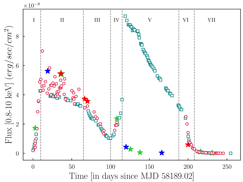
Figure 1: Light curve in the energy range $0.8-10$ keV generated using the NICER and XRT observations of MAXI J1820+070. The red circles represent the XRT data, and the green squares represent NICER data. The flux in the $10-60$ keV band for the simultaneous pairs for XRT-NuSTAR, NICER-NuSTAR and AstroSat observations are marked with red, green and blue stars respectively. Different evolutionary phases of the outbursts are marked from I to VII (see text for details).

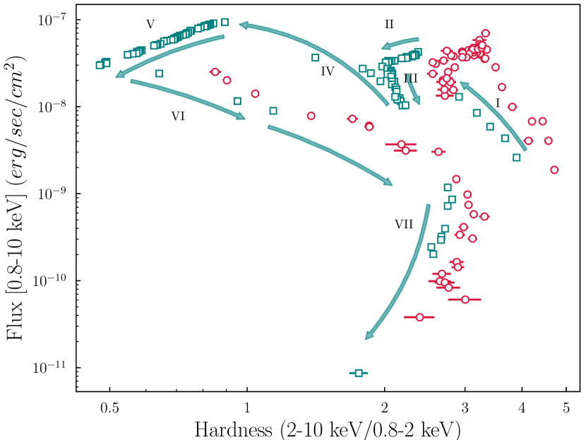
Figure 2: The Hardness-Intensity diagram of the source MAXI J1820+070 during the period MJD 58189 to MJD 58443. The hardness is calculated as the ratio of fluxes in $2-10$ keV to $0.8-2$ keV for both NICER and XRT. The red circles represent the XRT data, and green squares represent NICER data. Various phases (I-VII) of the light curve are marked. See text for details.

3.1 Spectral Analysis of Swift/XRT and NICER

We perform the spectral analysis of the source using Swift/XRT and NICER (though both operate in the similar energy range) independently to consider all the available observations in this energy range and scan the entire parameter space during both outbursts. Also, we aim for a comparative study of their spectral parameters. We use the software package XSPEC V12.10.1f and HEASOFT v6.26 for this analysis. The XSPEC absorption model tbabs, which adopts the solar abundance table given by Wilms et al. (2000), is used to account for the interstellar (ISM) absorption. We fixed $n_{H}=1.5\times 10^{21}\rm cm^{-2}$ (Uttley et al., 2018) for the line of sight column density throughout the study. The NICER and XRT observations are independently fitted in the energy range from 0.8 to 10 keV. The source is very bright, and we find residual in the NICER data below 0.8 keV (Fabian et al., 2020). Therefore, we ignore the data below 0.8 keV for NICER and XRT to keep a common energy range for the spectral analysis.

Figure 3: Evolution of (a) inner accretion disc temperature ($T_{in}$) and (b) disk normalization for XRT and NICER data. The red circles represent the XRT data, and the green squares represent NICER data. The uncertainties are within 90$\%$ confidence range. Different evolutionary phases are marked from I to VII. The star marks represent the values estimated from the wideband spectral analysis using phenomenological models discussed in §3.4.1.

We consider MJD 58189.02 as day 0 of the analysis, and henceforth all results are presented with respect to this reference date. At the very beginning of the Outburst-I and end stages of the Outburst-II, only a powerlaw component and the ISM absorption is enough to model (tbabs $\times$ powerlaw) the XRT data. However, an additional multicolor blackbody (diskbb) (Mitsuda et al., 1984) component is required to model (tbabs(diskbb+powerlaw)) the XRT data in-between. NICER data show a line signature around $6-7$ keV throughout all observations of Outburst-I. Therefore, we use a Gaussian profile (gauss) to represent the line and the overall model is tbabs(diskbb+powerlaw+gauss) during this period. For Outburst-II, the model tbabs(diskbb+powerlaw) is adequate for fitting the NICER data. We use $\chi^{2}$ statistics to represent the goodness of the fit. The $\chi^{2}/dof$ for all the XRT and NICER spectral fittings vary between $0.79-1.38$ and $0.72-1.33$ respectively. The uncertainties in the spectral fitting parameters are calculated within 90$\%$ confidence range using the modified Levenberg-Marquardt (leven) algorithm.

3.2 Outburst Profile and HID

We estimate the flux in $0.8-10$ keV range for individual XRT and NICER observations during MJD 58189 to MJD 58443. The light curve of the source in the energy range $0.8-10$ keV, generated using both NICER and XRT observations is shown in Fig. 1. The red circles represent the XRT data, and green squares represent NICER data. We notice that the overall fluxes of both instruments are comparable. As discussed in Appendix-A, there may be ($10-20$%) discrepancies in the estimated source flux due to calibration uncertainties in the spectral responses between both instruments. Also, a slight deviation may result due to the variation of the source itself as the XRT and NICER observations are not simultaneous. We marked different phases (I to VII) in the light curve to identify the evolution of the outburst. Since its discovery, MAXI J1820+070 showed an increase in flux with a short rise time (Phase-I) of $\sim$ 10 days (MJD 58200) to reach the peak and then started to decay slowly (Phase-II, also referred to as plateau phase) between $\sim$ $10-60$ days (MJD 58250) followed by a much steeper decline (Phase-III) till 100 days (MJD 58290). After this phase, Outburst-II is triggered, with a rapid increase in flux (Phase-IV), and at around day 110 (MJD 58300), the X-ray flux reached the second peak ($9.38\pm 0.01\times 10^{-8}$ erg/sec/cm²), approximately 1.5 times higher than the peak value of Outburst-I in $0.8-10$ keV band. Then the source flux decays linearly (Phase-V) for the next 80 days (MJD 58380), followed by an exponential decline of flux (Phase-VI). Finally, at around day 220 (MJD 58410) the source reached the quiescence (Phase-VII). We notice that the peak flux of Outburst-I in $2-10$ keV band is larger (a factor of 2.4 for NICER and 3 for XRT) than the flux in $0.8-2$ keV band, whereas the same for Outburst-II is lower by a factor of 1.2 (NICER). A similar trend is observed in $10-60$ keV band, represented by star symbols in Fig. 1, obtained from broadband spectral studies (see also Swift/BAT light curve in Fabian et al. (2020); Buisson et al. (2019), Insight-HXMT light curve in You et al. (2021); Ma et al. (2021)). Here red, green, and blue stars represent simultaneous pairs for XRT-NuSTAR, NICER-NuSTAR and AstroSat observations, respectively. It indicates that Outburst-I is harder in comparison with Outburst-II and we explore it in detail in §3.3. We use these simultaneous pairs of observations for broadband spectral studies in §3.4.

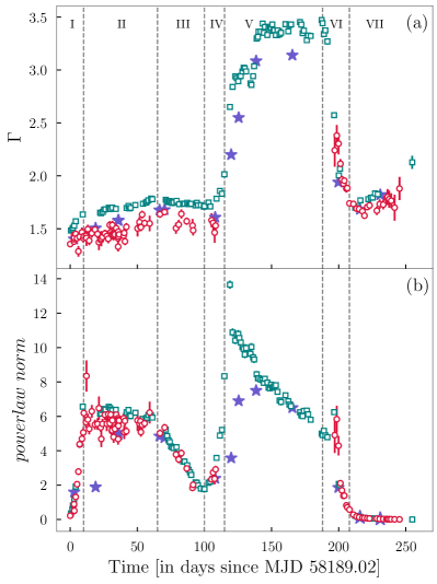
Figure 4: The time evolution of (a) photon index and (b) powerlaw normalization for XRT and NICER data. The red circles represent the XRT data, and the green squares represent NICER data. The uncertainties are within 90$\%$ confidence range. Different evolutionary phases are marked from I to VII. The star marks represent the same estimated from the wideband spectral analysis (§3.4.1) using phenomenological models.

We also estimate the flux in $0.8-2$ keV (low) and $2-10$ keV (high) separately for all XRT and NICER observations. We define the hardness (HR) as the ratio of flux in $2-10$ keV to that in $0.8-2$ keV. The hardness-intensity diagram for both outbursts are plotted in Fig. 2. Here also, the red circles represent the XRT data points and green squares represent the NICER data points. The HID of the two instruments show an offset in HR, particularly when the source is bright during Outburst-I. In comparison with XRT, the NICER flux is $\sim 10\%$ higher in the low energy band but $\sim 10\%$ lower in the hard energy band, maintaining a comparable total flux (See Appendix-A). This results in a $\sim 22\%$ lower HR for NICER data than XRT. We find that enhancing the NICER HR by this factor makes both HID comparable. We have marked various phases (I-VII) to indicate the evolution of the source in HID. The outburst starts with low luminosity LHS (Phase-I) with highest HR, and then evolves approximately at a constant flux level (Phase-II) with a significant change in HR. Then source flux decreases roughly at a constant HR (Phase-III) between $\sim$ $60-100$ days. During Outburst-I, the source remains only in the LHS (Phase-I to III in Fig. 2) and it is a ‘failed’ outburst. Outburst-II is triggered through Phase-IV (very short intermediate state) with an enhancement of flux, and the source reaches the HSS (Phase V). During the decline phase, the source returns to the LHS (Phase-VII) again via an intermediate state (Phase-VI), completing a q-shaped hysteresis cycle since the hard-to-soft transition occurs at a higher flux than soft-to-hard. It is a complete outburst since it covers all the spectral states.

3.3 Evolution of Spectral Parameters

We have modelled all the XRT and NICER data using a combination of the phenomenological models powerlaw, diskbb and gauss (required only for NICER data). We aim to study the evolution of the spectral parameters during the progress of the outbursts to understand the physical scenario of the accretion process and its geometry. Also, we attempt to compare the parameters estimated using both instruments.

We have presented the evolution of the diskbb parameters, namely, the inner disk temperature, $T_{in}$, in Fig. 3a and the diskbb normalization, diskbb norm, in Fig. 3b for both XRT and NICER. XRT data points are marked by the red circles and NICER by green squares, respectively. The uncertainties are within 90$\%$ confidence range. The star marks represent the values estimated from the wideband spectral analysis using phenomenological models discussed in §3.4.1. We see that the diskbb component is required to model all observations of Outburst-I (first $\sim 100$ days). Inner disk temperature is low at the beginning of the outburst, and it increases as the accretion of matter increases in the brief rising phase ($\sim 10$ days). Both $T_{in}$ and diskbb norm remain almost constant (though two parameters from XRT data show some random variation) during Phase-II, although a slow decline (Phase-III) is observed towards the end of Outburst-I. It means the thermal component does not change much in Phase-II while it slowly decreases (Phase-III) in the decline part of the Outburst-I. The diskbb norm is directly proportional to the inner radius of the accretion disk, $R_{in}$. The source was in the LHS during Outburst-I and the high value of diskbb norm indicates that the disk is truncated at a large radius (see also, Zdziarski et al. (2021a); Zdziarski et al. (2021b)).

Around day 100 (MJD 58290), the Outburst-II is triggered and the source becomes extremely luminous with a very sharp increase of $T_{in}$ ($\sim$ factor of 3) and order of magnitude decrease in diskbb norm. The source transits to the HSS via a very brief intermediate state. The large value of $T_{in}$ signifies strong accretion activity and the low value of diskbb norm reveals that the inner edge of the accretion disk extends close to the central object. Also, the approximately constant value of diskbb norm during the HSS indicates that $R_{in}$ does not evolve during this period. However, $T_{in}$ gradually decreases along with the decline of the source flux. The evolution of the source in this phase is regulated by the thermal component of the radiation. As mentioned earlier, we have ignored the XRT observations during this period due to huge pile-up issues and have used NICER data for spectral modelling. As the source returns back to the LHS, $T_{in}$ declines to a low value, and eventually, the contribution from the disk becomes insignificant after $\sim$ 210 days (MJD 58400). The outburst ends with the disk truncated again at a large distance and diskbb norm becomes large.

Generally, it is proposed in the literature (Sunyaev & Titarchuk, 1980; Zdziarski et al., 1994; Sunyaev & Titarchuk, 1985; Titarchuk, 1994) that the origin of non-thermal component is due to the inverse-Comptonization of the soft thermal photons from the accretion disk by the ‘hot’ electrons in the corona. We use a powerlaw model to quantify the contribution of the non-thermal component. The evolution of the powerlaw model components are shown in Fig. 4. The XRT and NICER data are shown in red circles and green squares respectively as before. Fig. 4a represents the evolution of photon index ($\Gamma$) with time, whereas Fig. 4b shows the evolution of powerlaw normalization. Again the star marks represent the same estimated from the wideband spectral analysis using phenomenological models (See §3.4.1). In LHS, the contribution of Comptonized hard photons is larger than the soft disk photons and therefore, $\Gamma$ is low (harder spectrum) with a high value of powerlaw norm. We notice two distinct patterns of evolution of the powerlaw component in the LHS. Phase-II shows a gradual increase in $\Gamma$ (Fig. 4a) with a constant powerlaw norm (Fig. 4b) such that the light curve appears as a plateau (Fig. 1). However, $\Gamma$ remains constant and a gradual decline of powerlaw norm is observed in Phase-III. In both cases, there is a gradual decrease in the non-thermal flux. In the former case, the steepening of the spectral index due to steady thermal photon flux reduces the non-thermal flux, while in the latter case, it decreases due to the reduction of thermal photon flux without changing the nature of the non-thermal spectrum. Therefore, the thermal component does not change much and the non-thermal radiation regulates the dynamics in Phase-II, whereas both changes slowly in Phase-III of Outburst-I. We notice that $\Gamma$ (Fig. 4a) measured from NICER is higher ($\sim$ 0.24) than that of XRT during the LHS (Outburst-I) due to the difference in the instrumental response as discussed in Appendix-A. In Outburst-II, the spectrum is very soft ($\Gamma>3$) as the source enters the HSS very fast and its nature remains similar during the entire HSS (Phase-V) though the non-thermal flux reduces (powerlaw norm reduces) with time. In the declining phase, the source moves through the intermediate state ($\Gamma\sim 2$) and finally reaches the LHS (Phase-VII) with a hard spectrum.

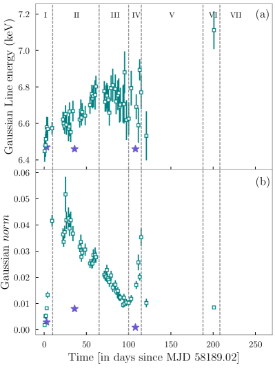
Figure 5: Time evolution of (a) Gaussian line energy and (b) Gaussian line normalization obtained from NICER data. The uncertainties are within 90$\%$ confidence range. Different evolutionary phases are marked from I to VII. The star marks represent the parameters estimated from the wideband spectral analysis (§3.4.1) using phenomenological models.

The spectral modelling of NICER data show an excess residual in $6-7$ keV range which is generally assumed to be Fe $K_{\alpha}$ feature produced due to the reflection of hard photons onto the cold accretion disk. We use a Gaussian profile wherever the feature is visible. The evolution of Fe $K_{\alpha}$ line energy (Fig. 5a) and the Gaussian normalization (Fig. 5b) estimated using NICER data are represented by green square. The star marks show the same from the broadband spectral modelling. The Gaussian line width for NICER is frozen at 0.6 keV for some observations, which unless giving very high values. At the beginning of the outburst, the source is in LHS and more hard powerlaw photons from the corona illuminate the accretion disk surface. We notice an increasing line contribution during the rising phase. Then there is a gradual decrease of powerlaw photons which results in a decrease in the amount of reflected radiation. This trend can be clearly visible in Fig. 5b. There are other factors, like, the slope of the hard photon spectrum from the corona, the ionization of the disk surface, etc. (Buisson et al., 2019; Kara et al., 2019; Axelsson & Veledina, 2021) are also responsible for the observed changes in the iron line profile. The Fe $K_{\alpha}$ line emission energy is 6.4 keV but it can vary slightly due to the relativistic effects. Fig. 5a shows the systematic increase of the Gauss line energy and it lies in the range $6.53-6.89$ keV. In Outburst-II, the source immediately enters the HSS, the disk photons dominate and further no more line features visible in the spectra. Although the NICER observation around $\sim$ 200 day shows a reflection feature at $\sim$ 7.1 keV.

Table 2: Simultaneous broadband (XRT-NuSTAR, NICER-NuSTAR and AstroSat) observations of the source MAXI J1820+070

Epoch	Obs. ID (MJD)
	NuSTAR	XRT	NICER	AstroSat
1	90401309002 (58191.94)		1200120103 (58190.99)
2				9000001994 (58208)
3	90401309013 (58224.95)	00010627042 (58224.87)
4	90401309013 (58224.95)	00010627043 (58224.95)
5	90401309014 (58225.28)		1200120131 (58225.03)
6	90401309019 (58255.60)	00088657004 (58255.90)
7	90401324002 (58259.24)	00010627062 (58259.35)
8	90401309021 (58297.17)		1200120189 (58297.19)
9				9000002216 (58309)
10	90401309025 (58314.75)		1200120207 (58314.19)
11	90401309027 (58327.05)		1200120220 (58327.89)
12				9000002324 (58355)
13	90401309033 (58388.91)	00088657010 (58388.92)
14	90401309037 (58404.95)		1200120277 (58405.20)
15	90401309039 (58420.05)		1200120290 (58420.05)

3.4 Simultaneous Wideband Spectral Modelling

We have performed the simultaneous wideband spectral analysis of four different instruments, Swift/XRT, NICER, NuSTAR, and AstroSat to understand the spectral characteristics over a broad range. We consider all simultaneous or quasi-simultaneous (with a time difference not exceeding 1 hour) observations (XRT-NuSTAR, NICER-NuSTAR and AstroSat SXT-LAXPC) which are listed in Table 2. We used XRT or NICER data for the low energy band ($0.8-10$ keV), and NuSTAR data ($4-75$ keV) for the high energy regime. For AstroSat, we use SXT ($0.7-8$ keV) and LAXPC ($3-60$ keV) for the broadband simultaneous spectral modelling. The SXT data below 1.3 keV for Obs. ID 9000001994 (Epoch 2 in Table 2) show a high systematic residual, which is also reported by Chakraborty et al. (2020). Therefore, we have used SXT data between 1.3 - 7.0 keV for this observation. Temporal filter is applied to the simultaneous NuSTAR data according to the exposure time of the corresponding XRT/NICER observation to ensure they are strictly simultaneous. The spectra from both focal plane modules (FPMA and FPMB) of NuSTAR data are fitted together. A normalization constant is used to account for the calibration difference, if any, between FPMA and FPMB.

We consider 15 epochs (5 pairs of XRT-NuSTAR, 3 pairs of AstroSat and 7 pairs of NICER-NuSTAR) of simultaneous data (Table 2) and model them using combination of phenomenological models for a comparison of parameters obtained from the spectral modelling of individual NICER/XRT data. Also, we model the broadband data using reflection model to estimate the accretion disk characteristics, BH spin, inclination angle etc. The $n_{H}$ value is fixed at 1.5$\times 10^{21}\rm cm^{-2}$, same as the XRT/NICER spectral modelling (§3.1). AstroSat/LAXPC data show an instrumental feature $\sim 30$ keV due to Xe K fluorescence X-rays since the detector is filled with a mixture of xenon and methane (Antia et al., 2017, 2021; Sreehari et al., 2019). Additional absorption edges are used in order to address this instrumental feature of LAXPC.

Table 3: Spectral parameters of simultaneous broadband X-ray data (XRT-NuSTAR, NICER-NuSTAR and AstroSat) fitted with phenomenological models. The XRT-NuSTAR pairs and AstroSat observations are highlighted with dark-grey and pale-gray colors, respectively; others are NICER-NuSTAR pairs. The uncertainties are within 90$\%$ confidence range.

Epoch	Model									$\chi^{2}_{red}$
	diskbb		gauss			smedge		powerlaw
	$T_{in}$	norm	line E	sigma	norm	edge E	width	$\Gamma$	norm
	(keV)	($\times 10^{4}$)	(keV)	(keV)	(photons/cm2/s)	(keV)	(keV)		(photons/keV/cm2/s)
1	$0.26_{-0.01}^{+0.01}$	$1.2_{-0.3}^{+0.3}$	$6.47_{-0.04}^{+0.04}$	$0.25_{-0.05}^{+0.05}$	$0.0029_{-0.0005}^{+0.0006}$	$6.57_{-0.09}^{+0.08}$	$8.9_{-1.7}^{+2.4}$	$1.403_{-0.002}^{+0.002}$	$1.6_{-0.3}^{+0.4}$	1.17
2	$0.391_{-0.002}^{+0.003}$	$1.62_{-0.13}^{+0.09}$	—	—	—	$8.1_{-0.3}^{+0.3}$	$3.8_{-0.9}^{+0.4}$	$1.506_{-0.001}^{+0.009}$	$4.37_{-0.06}^{+0.06}$	1.43
3	$0.23_{-0.01}^{+0.01}$	$17.5_{-4.8}^{+6.9}$	—	—	—	$7.24_{-0.09}^{+0.09}$	$3.7_{-0.6}^{+0.8}$	$1.578_{-0.003}^{+0.003}$	$4.93_{-0.03}^{+0.03}$	1.33
4	$0.22_{-0.02}^{+0.02}$	$16.2_{-5.3}^{+8.3}$	—	—	—	$7.2_{-0.1}^{+0.1}$	$3.7_{-0.6}^{+0.8}$	$1.578_{-0.003}^{+0.003}$	$4.94_{-0.03}^{+0.03}$	1.28
5	$0.325_{-0.003}^{+0.003}$	$6.04_{-0.2}^{+0.2}$	$6.46_{-0.03}^{+0.03}$	$0.28_{-0.03}^{+0.03}$	$0.0083_{-0.0008}^{+0.0008}$	$7.33_{-0.06}^{+0.06}$	$3.2_{-0.3}^{+0.4}$	$1.580_{-0.001}^{+0.001}$	$5.05_{-0.01}^{+0.01}$	1.89
6	$0.19_{-0.01}^{+0.01}$	$58.2_{-18.6}^{+28.9}$	—	—	—	$7.2_{-0.1}^{+0.1}$	$4.4_{-1.1}^{+1.6}$	$1.677_{-0.004}^{+0.004}$	$4.85_{-0.04}^{+0.04}$	1.06
7	$0.21_{-0.01}^{+0.01}$	$29.5_{-7.6}^{+10.7}$	—	—	—	$7.2_{-0.2}^{+0.2}$	$4.8_{-1.5}^{+2.4}$	$1.68_{-0.01}^{+0.01}$	$4.76_{-0.04}^{+0.04}$	1.10
8	$0.325_{-0.002}^{+0.002}$	$3.7_{-0.1}^{+0.1}$	$6.46_{-0.04}^{+0.04}$	$0.12_{-0.05}^{+0.05}$	$0.0009_{-0.0002}^{+0.0002}$	$7.33_{-0.04}^{+0.04}$	$5.1_{-0.4}^{+0.5}$	$1.608_{-0.001}^{+0.001}$	$2.395_{-0.006}^{+0.006}$	1.55
9	$0.7_{-1.1}^{+0.6}$	$2.25_{-0.02}^{+0.03}$	—	—	—	$7.58_{-0.07}^{+0.07}$	$16.5_{-1.1}^{+0.6}$	$2.20_{-0.01}^{+0.01}$	$3.58_{-0.08}^{+0.09}$	1.7
10	$0.713_{-0.001}^{+0.001}$	$1.89_{-0.02}^{+0.02}$	—	—	—	$6.87_{-0.05}^{+0.06}$	$14.3_{-3.1}^{+3.2}$	$2.55_{-0.01}^{+0.02}$	$6.9_{-0.2}^{+0.2}$	1.42
11	$0.711_{-0.001}^{+0.001}$	$1.66_{-0.02}^{+0.02}$	—	—	—	$6.76_{-0.08}^{+0.08}$	$13.9_{-0.4}^{+0.9}$	$3.086_{-0.017}^{+0.006}$	$7.5_{-0.2}^{+0.2}$	1.09
12	$0.618_{-0.002}^{+0.002}$	$2.01_{-0.04}^{+0.04}$	—	—	—	$8.9_{-0.3}^{+0.4}$	$8.84^{{\dagger}}$	$3.14_{-0.02}^{+0.02}$	$6.5_{-0.2}^{+0.2}$	1.80
13	$0.35_{-0.01}^{+0.01}$	$3.0_{-0.3}^{+0.4}$	—	—	—	$7.8_{-0.2}^{+0.2}$	$13.87^{{\dagger}}$	$1.94_{-0.02}^{+0.01}$	$1.86_{-0.05}^{+0.05}$	1.03
14	$0.20_{-0.02}^{+0.02}$	$0.3_{-0.1}^{+0.2}$	—	—	—	—	—	$1.683_{-0.009}^{+0.009}$	$0.124_{-0.003}^{+0.003}$	0.97
15	—	—	—	—	—	—	—	$1.821_{-0.006}^{+0.006}$	$0.0383_{-0.0005}^{+0.0006}$	1.00

• †Parameter uncertainty can’t be estimated.

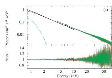
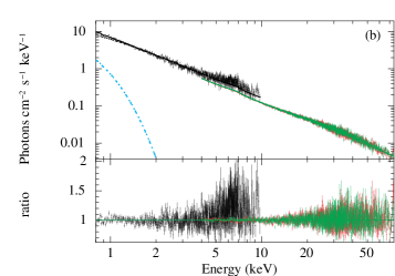
Figure 6: (a) Simultaneous NICER-NuSTAR observation at MJD 58191 (Epoch 1 in Table 2) fitted using the model tbabs(diskbb+relxilllpCp). Black color represents NICER data and red and green for NuSTAR FPMA and FPMB respectively. (b) Quasi-Simultaneous XRT-NuSTAR observation at MJD 58224 (Epoch 3 in Table 2) fitted using the model tbabs(diskbb+relxilllpCp). Black color represents XRT data and red and green for NuSTAR FPMA and FPMB, respectively. The diskbb and reflection components are shown in light blue and black dotted lines, respectively.

3.4.1 Phenomenological Spectral Modelling

We have attempted to model the XRT-NuSTAR, NICER-NuSTAR and AstroSat observations using a combination of the phenomenological models diskbb and nthcomp with a motivation to estimate the temperature of the corona and exponential cut-off, if any. But we could neither constrain the electron temperature nor the cut-off energy. Therefore, we continue to model the broadband data with diskbb and powerlaw to maintain a consistency with the spectral modelling of individual NICER/XRT data. Additionally, we have used components like gauss and smedge if they are required. The estimated parameters are presented in Table 3 and marked with star symbol in Fig. 3,4,5. The diskbb parameters are consistent with NICER/XRT, though Epoch 2 (AstroSat) records a higher $T_{in}$ and lower diskbb norm than NICER/XRT. Epoch $1-8$ and Epoch $14-15$ in Table 3 belong to LHS and the estimated powerlaw index is consistent with the same from XRT data alone (Fig. 4a). Epoch $9-12$ corresponds to HSS and the estimated $\Gamma$ ($\lesssim 3$) is significantly harder than that estimated from the NICER data (Fig. 4a). During Epoch 13, the source was possibly transiting through an intermediate state with $\Gamma=1.94_{-0.02}^{+0.01}$. Additional Gausian component is required for three broadband (Epoch 1, 5 & 8 in Table 3) observations and the line parameters differ significantly from that of NICER data (Fig. 5). This is because NuSTAR has a broad coverage to capture the reflection features and has a better energy resolution in this range. Inclusion of NuSTAR data results in constraining the gauss line energy and width (Table 3) better than NICER data alone. We also notice the presence of absorption edge ($6.75-9.3$ keV) in all the simultaneous data except Epochs 14 and 15 (towards the quiescent state). It possibly indicates that significant amount of hard X-ray irradiation is present during the outbursts.

3.4.2 Spectral Modelling for Reflection Features

The hard X-ray photons from the corona can irradiate the accretion disk surface, getting reprocessed by absorption and down scattering, producing a reflection signature in the observed data. Therefore, X-ray reflection spectroscopy is a powerful tool for studying the accretion disk characteristics such as the degree of ionization and the elemental abundances. The reflection lines suffer relativistic broadening and its shape depends on spin of the BH, the inclination of the accretion disk, geometry of the corona, etc. (Dauser et al., 2013). Therefore, the study of the relativistic reflected spectrum is a direct probe towards the physics around the strong gravity region and we can determine the spin of the BH and the inclination of the system, in addition to the accretion disk characteristics. Generally, the reflection models assume a primary spectrum, either a broken powerlaw emissivity (in case of extended corona) or an isotropic point-like source at a given height (lamp-post corona) on the rotation axis of the BH. There are studies related to reflection features in the spectra of MAXI J1820+070 on a selected number of observations using various flavors of reflection models (Buisson et al., 2019; Chakraborty et al., 2020; Buisson et al., 2021; Marino et al., 2021; You et al., 2021; Kawamura et al., 2022).

In our study, we have performed broadband spectral modelling using a few different flavors of the relativistic reflection model RELXILL such as relxilllpCp, relxilllp (García et al., 2014). This model uses the transfer function method (Cunningham, 1975) to calculate the photon trajectory from the point of emission in the accretion disk to the observer (a ray-tracing code). The model takes care of the proper emission angle at each point on the disk and calculates the reflected flux, instead of following an angle-averaged method. The relxilllpCp model assumes a lamp-post geometry for the corona and nthcomp continuum (Dauser et al., 2014) for the incident primary spectrum, whereas in relxilllp model a cut-off powerlaw continuum is considered as the primary spectrum with the same coronal geometry.

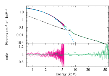
Figure 7: Broadband energy spectrum of AstroSat observation (Epoch 9) is best fitted with the model tbabs(diskbb+relxilllp). The SXT and LAXPC data are plotted in magenta and green color, respectively. The diskbb and reflection components are shown in light blue and black dotted lines respectively.

Table 4: Spectral parameters of simultaneous broadband XRT-NuSTAR, NICER-NuSTAR and AstroSat observations fitted using RELXILL group of models. The XRT-NuSTAR pairs and AstroSat observations are highlighted with dark-grey and pale-gray colors respectively, others are NICER-NuSTAR pairs. The uncertainties are within 90$\%$ confidence range.

Epoch	Model										$\chi^{2}_{red}$
	diskbb		relxilllpCp
	$T_{in}$	norm	h	$\theta$	$\Gamma$	$log$ $\xi$	$A_{Fe}$	$R_{f}$	$kT_{e}$	norm
	(keV)	($\times 10^{4}$)	$(GM/c^{2})$	(deg)		(erg cm s-1)	($A_{Fe,\odot}$)		(keV)	($\times 10^{-2}$)
1	$0.237_{-0.002}^{+0.007}$	$1.59_{-0.2}^{+0.2}$	$202.25_{-64.2}^{+159.01}$	$63.0^{{\dagger}{\dagger}}$	$1.553_{-0.001}^{+0.003}$	$2.01_{-0.06}^{+0.08}$	$2.4_{-0.1}^{+0.1}$	$0.39_{-0.01}^{+0.01}$	$100.0^{{\dagger}{\dagger}}$	$5.9_{-0.1}^{+0.1}$	1.09
2	$0.33_{-0.02}^{+0.02}$	$2.3_{-0.5}^{+0.6}$	$100.0^{{\dagger}{\dagger}}$	$63.0^{{\dagger}{\dagger}}$	$1.54_{-0.01}^{+0.01}$	$3.70_{-0.04}^{+0.07}$	$4.4_{-0.8}^{+2.5}$	$0.7_{-0.3}^{+0.2}$	$100.0^{{\dagger}{\dagger}}$	$16.5_{-1.7}^{+2.8}$	1.46
3	$0.17_{-0.02}^{+0.02}$	$44.6_{-22.5}^{+51.8}$	$29.46_{-9.55}^{+10.36}$	$56.9_{-7.0}^{+9.6}$	$1.72_{-0.01}^{+0.01}$	$1.69^{\dagger}$	$2.4_{-0.3}^{+0.3}$	$0.6_{-0.1}^{+0.2}$	$116.67^{\dagger}$	$18.2_{-0.9}^{+1.5}$	1.20
4	$0.17_{-0.02}^{+0.02}$	$47.1_{-27.0}^{+53.6}$	$30.44_{-4.84}^{+6.88}$	$59.8_{-3.7}^{+4.3}$	$1.73_{-0.01}^{+0.01}$	$1.70_{-0.09}^{+0.05}$	$2.3_{-0.1}^{+0.4}$	$0.61_{-0.09}^{+0.14}$	$100.0^{{\dagger}{\dagger}}$	$17.6_{-0.7}^{+0.8}$	1.14
5	$0.296_{-0.003}^{+0.002}$	$7.02_{-0.4}^{+0.5}$	$30^{\dagger}$	$63.0^{{\dagger}{\dagger}}$	$1.729_{-0.003}^{+0.002}$	$1.70_{-0.02}^{+0.01}$	$2.14_{-0.06}^{+0.09}$	$0.67_{-0.01}^{+0.01}$	$100.0^{{\dagger}{\dagger}}$	$18.0_{-0.1}^{+0.1}$	1.13
6	$0.16_{-0.01}^{+0.01}$	$105.9_{-53.7}^{+100.4}$	$23.1_{-3.3}^{+4.5}$	$63.0^{{\dagger}{\dagger}}$	$1.808_{-0.004}^{+0.004}$	$1.70_{-0.03}^{+0.02}$	$2.7_{-0.2}^{+0.4}$	$0.65_{-0.03}^{+0.02}$	$100.0^{{\dagger}{\dagger}}$	$13.7_{-0.3}^{+0.2}$	1.08
7	$0.17_{-0.01}^{+0.01}$	$58.4_{-21.6}^{+22.9}$	$23.1_{-4.6}^{+5.5}$	$63.0^{{\dagger}{\dagger}}$	$1.82_{-0.01}^{+0.01}$	$1.70_{-0.04}^{+0.02}$	$2.7_{-0.2}^{+0.5}$	$0.67_{-0.03}^{+0.06}$	$100.0^{{\dagger}{\dagger}}$	$13.2_{-0.2}^{+0.3}$	1.11
8	$0.306_{-0.001}^{+0.003}$	$4.0_{-0.1}^{+0.2}$	$20.3_{-1.2}^{+0.6}$	$63.0_{-0.6}^{+0.4}$	$1.741_{-0.001}^{+0.001}$	$1.699_{-0.003}^{+0.003}$	$2.81_{-0.07}^{+0.05}$	$0.59_{-0.02}^{+0.03}$	$100.0^{{\dagger}{\dagger}}$	$8.57_{-0.03}^{+0.05}$	1.52
9∗	$0.710_{-0.002}^{+0.002}$	$1.91_{-0.03}^{+0.04}$	$3.0_{-0.5}^{+0.5}$	$63.0^{{\dagger}{\dagger}}$	$2.32_{-0.03}^{+0.02}$	$3.09_{-0.03}^{+0.04}$	$10.0^{{\ddagger}}$	$3.6_{-0.2}^{+0.3}$	—	$14.8_{-4.4}^{+8.8}$	1.58
10∗	$0.7398_{-0.001}^{+0.001}$	$1.67_{-0.02}^{+0.02}$	$2.0^{{\ddagger}}$	$63.0^{{\dagger}{\dagger}}$	$2.57_{-0.01}^{+0.01}$	$3.31_{-0.01}^{+0.02}$	$7.9_{-1.5}^{+1.1}$	$3.10_{-0.03}^{+0.27}$	—	$125.3_{-1.1}^{+9.0}$	1.19
11∗	$0.7198_{-0.001}^{+0.001}$	$1.67_{-0.003}^{+0.003}$	$2.23_{-0.02}^{+0.04}$	$59.9_{-0.4}^{+0.3}$	$3.273_{-0.050}^{+0.003}$	$2.70_{-0.02}^{+0.01}$	$10.0^{{\ddagger}}$	$3.8_{-0.1}^{+0.1}$	—	$424.5_{-4.6}^{+126}$	1.28
12∗	$0.691_{-0.002}^{+0.002}$	$0.55_{-0.01}^{+0.01}$	$2.69_{-0.45}^{+0.45}$	$63.0^{{\dagger}{\dagger}}$	$3.12_{-0.01}^{+0.01}$	$4.3_{-0.06}^{+0.06}$	$10.0^{{\ddagger}}$	$3.59_{-0.37}^{+0.37}$	—	$15.8_{-1.0}^{+1.0}$	1.37
13	$0.35_{-0.01}^{+0.01}$	$2.38_{-0.4}^{+0.4}$	$11.25_{-2.26}^{+3.65}$	$63.0^{{\dagger}{\dagger}}$	$2.07_{-0.02}^{+0.02}$	$1.7_{-0.1}^{+0.2}$	$4.7_{-0.7}^{+0.4}$	$0.8_{-0.1}^{+0.1}$	$100.0^{{\dagger}{\dagger}}$	$3.9_{-0.2}^{+0.5}$	1.10
14	—	—	$8.6^{\dagger}$	$63.0^{{\dagger}{\dagger}}$	$1.73_{-0.01}^{+0.01}$	$2.8_{-0.1}^{+0.1}$	$1.4_{-0.5}^{+0.7}$	$0.38_{-0.04}^{+0.05}$	$54.34^{\dagger}$	$0.5_{-0.1}^{+0.2}$	1.0
15	—	—	$3.03^{{\dagger}}$	$63.0^{{\dagger}{\dagger}}$	$1.84_{-0.01}^{+0.01}$	$1.7_{-0.6}^{+0.2}$	$5.0_{-1.2}^{+2.4}$	$0.38_{-0.07}^{+0.07}$	$100.0^{{\dagger}{\dagger}}$	$0.38_{-0.004}^{+0.003}$	0.98

• * HSS where relxilllp model is used instead of relxilllpCp. Here, $kT_{e}$ is not a parameter and norm is the relxilllp normalization.

• †Parameter uncertainty can’t be estimated.

• ††Frozen parameter.

• ‡Parameter hits the boundary.

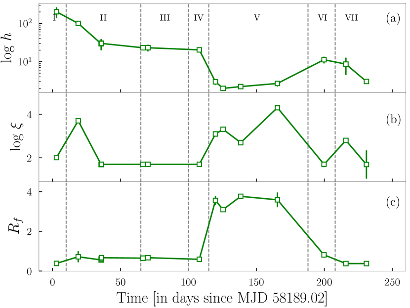
Figure 8: Evolution of the reflection parameters: (a) lamp-post height (h), (b) ionization parameter ($log$ $\xi$) and (c) reflection fraction ($R_{f}$) obtained from simultaneous wideband spectral study. Different evolutionary phases are marked from I to VII.

In the reflection modelling, we mainly use a combination of diskbb and relxilllpCp models to fit the data except Epoch $9-12$. During these four epochs, which are in the HSS, relxilllpCp model did not produce a good fit and value of few parameters become unphysical. Therefore, we use relxilllp for a better spectral fitting. We present the simultaneous NICER-NuSTAR (Epoch 1) and XRT-NuSTAR (Epoch 3) broadband reflection modelling in Fig. 6a and Fig. 6b respectively. We use the model tbabs(diskbb+relxilllpCp) to fit the data for both cases. Black color represents the XRT data in Fig. 6a and NICER data in Fig. 6b, whereas red and green are for NuSTAR FPMA and FPMB respectively. Fig. 7 represents the AstroSat observation (Epoch 9) fitted with the model tbabs(diskbb+relxilllp). Here, SXT and LAXPC data are shown in magenta and green colors, respectively. As thermal disk component is needed for the low energy data. Note that in phenomenological modelling (§3.4.1), the reflection features are managed by a gaussian component at $\sim$ 6.4 keV and smedge component $\sim$ 7 keV for most of the epochs. On the other hand, reflection features such as iron line, edge and the Compton hump are self-consistently calculated in the RELXILL model.

Similarly, all the pairs in Table 2 are fitted with RELXILL models. The important parameters are estimated and are summarised in Table 4, while other parameters are frozen at their default values. The uncertainties are within 90$\%$ confidence range. The inner disk temperature, $T_{in}$ and photon index, $\Gamma$ estimated for each epoch from phenomenological (Table 3) and reflection modelling (Table 4) are generally agreed well. However, $T_{in}$ estimated from reflection modelling is marginally lower, $\Gamma$ is a little on the higher side. A possible reason could be that the soft-excess from the reflection model provides a small contribution towards lower energy reducing the temperature of the diskbb component. Also, the primary spectrum may become marginally softer since the reflection reduces the number of hard X-ray primary photons.

The spin parameter $a_{\ast}$ is found to be pegged near the highest allowed limit, therefore we freeze $a_{\ast}=0.998$. Bhargava et al. (2021) predicted the BH spin of MAXI J1820+070 as $0.799^{+0.016}_{-0.015}$ using timing study, but they expected an underestimation in the calculation and this value should be regarded as a lower limit. Therefore, the high spin approximation that we have used in our study is justified. The inclination angle, $\theta$, of the system is estimated to be $63^{\circ}$ (Atri et al., 2020). We could able to estimate the inclination angle for few observations (Epoch 3, 4, 8 and 11). Otherwise, we freeze $\theta=63^{\circ}$, since we cannot constrain it from the fitting. The inner radius of the accretion disk $R_{in}$ is fixed at $R_{ISCO}$, the innermost stable circular orbit radius, and outer radius $R_{out}$ is frozen at the default value (400 $r_{g}$, where $r_{g}\equiv GM/c^{2}$, the gravitational radius of the BH). In most of cases the electron temperature in the corona $kT_{e}$ is hitting the upper boundary, therefore in such cases, we freeze it to a more reasonable value of 100 keV. We used lamp-post height $h$, inclination angle $\theta$, photon index of the incident radiation $\Gamma$, ionization parameter log($\xi$), iron abundance ($A_{Fe}$) of the accretion disk in terms of the solar abundance, and reflection fraction $R_{f}$ as the free parameters. $R_{f}$ is defined as the ratio of intensity of the primary photons illuminating the disk to that reach the observer (Dauser et al., 2016). This parameter depends on the strength of the reflection component and the geometry of the system.

The evolution of the reflection parameters is shown in Fig. 8. The number of primary source photons illuminating the disk increases in the rising phase of the outburst and hence the ionization ($log$ $\xi$) (Fig. 8b) of the disk material increases.

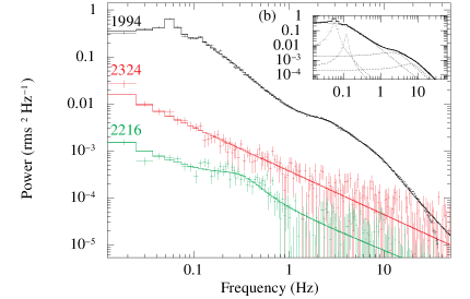
Figure 9: Representation of PDS for (a) NICER observation on day 56.43, fitted using multiple Lorentzian components and (b) AstroSat observations are shown. Three AstroSat observations on Epoch 2, 9, 12 (Table 2) are plotted in black, green, and red colors respectively. The Lorentzian components for Epoch 2 are shown in the inset.

As a result, the amount of reflection, $R_{f}$, increases during the rising phase of Outburst-I. Therefore, $R_{f}$ shows a positive correlation with the luminosity of the source in the hard state (Atri et al., 2020). During Phase-II, the lamp-post height, $log$ $\xi$, and $R_{f}$ decrease from the rising phase whereas in Phase-III, these parameters remain steady. $R_{f}$ shows a slight decrease for Epoch 8 (Phase-IV) which is the very beginning of the second outburst and has low flux. However, You et al. (2021) considered a lamp-post corona for the hard state of MAXI J1820+070 and reported an unusual decreasing trend in the reflection fraction due to the effect of the bulk motion of the corona. We are considering a point-like static lamp-post corona, where this effect is not coming into the picture. Thermal reverberation lags (De Marco et al., 2021) showed that the relative distance between the primary photon source and the disc decreases as the source softens.

Dauser et al. (2016) found that reflection is strong for low source height (h) and high inclination. In the HSS (Phase-V in Fig. 8), we find corona is close to the central object with a high reflection fraction $R_{f}\sim 3.5$, high ionization parameter ($log$ $\xi$ $\sim 4$) and over-abundance of iron ($A_{Fe}$). Buisson et al. (2019) and Bharali et al. (2019) also reported the chances of overestimation of $A_{Fe}$. During the decline phase (Epoch $13-15$) shows a reduction of ionization and reflection fraction. The lamp-post height shows a momentary increase (Epoch 13) when the hard flux takes over the soft flux and then declines as the source becomes faint. Thus, the broadband reflection modelling shows the presence of a dynamically evolving corona (lamp-post hight is changing) during both outbursts except in the HSS.

3.5 Temporal Analysis and Modelling

For the timing analysis of MAXI J1820+070, we consider all the NICER data of the source and the three available AstroSat/LAXPC observations during this period. We generate light curves for NICER observations with more than 1 ks exposure, with a binsize of 3 ms in the full energy range. We did not subtract any background from the light curve and generated PDS using the tool powspec. The PDS are Poisson noise subtracted (Zhang et al., 1995) and normalized to squared RMS fractional variability. For Outburst-I, we have rebinned the data such that $f_{min}=0.01$ Hz and $f_{max}=55.55$ Hz. A geometrical rebinning factor of -1.09 is applied. For Outburst-II, particularly for the soft state data, we prefer a larger binsize to get a good statistics and we have $f_{min}=0.001$ Hz and $f_{max}=2.564$ Hz. Here, we rebin the PDS with a geometrical rebinning factor of -1.2. For AstroSat/LAXPC data, we create light curve with a time resolution of 0.1 sec in the $3-60$ keV energy band. The PDS is geometrically rebinned by a factor of -1.03. For the observation ID 9000002216 (Epoch 2, in Table 2), the PDS is made only from segments 10-19 since the other segments are having low exposure time.

We generated a flat response and use XSPEC to model the PDS. The broad noise features in the PDS are modelled with zero-centered Lorentzians. We also use powerlaw components for fitting the PDS in the HSS observations only, since the PDS are almost featureless. We use a combination of Lorentzian in order to identify the QPOs or QPO-like features in the PDS. The functional form of Lorentzian in XSPEC is written as,

$$L(\nu)=\frac{K}{\pi}\frac{\Delta}{(\nu-\nu_{c})^{2}+\Delta^{2}}\rm,$$ (1)

where $\nu$ is the frequency and $\nu_{c}$ (characteristic frequency of QPO) is the line centre. Here, $\Delta$ is the half width at half maximum (HWHM) of the line and $K$ is the normalization. All the three Lorentzian parameters ($\nu_{c}$, $\Delta$, and $K$) of the QPO-like features are estimated for each observation. For each Lorentzian, we calculate Q-factor ($Q=\nu_{c}/2\Delta$) and significance, which is defined as the ratio of Lorentzian normalization to its negative error (Alam et al., 2014; Sreehari et al., 2019). The area under a Lorentzian is given by,

$$I=\frac{K}{2}\left[1+\frac{2}{\pi}\ tan^{-1}\left(\frac{\nu_{c}}{\Delta}\right)\right],$$ (2)

and the fractional RMS amplitude is calculated as $\sqrt{I}$. The total RMS of each PDS is also computed by integrating the whole PDS over frequency (Casella et al., 2005; Belloni, 2010; Motta et al., 2011; Motta et al., 2012).

Typical example of fitted PDS for NICER observations on day 56.43 is shown in Fig. 9a. Here, the PDS is fitted using multiple Lorentzian profiles. The feature at $\nu_{c}$=$0.42_{-0.02}^{+0.01}$ Hz is a QPO with Q-factor $3.19\pm 1.4$, significance 2.3 and fractional RMS (in percentage) is $5.9\pm 0.6$. In Fig. 9b, we present PDS correspond to the AstroSat observation IDs 9000001994 (Epoch 2), 9000002216 (Epoch 9), and 9000002324 (Epoch 12) in black, green, and red colors respectively. Various Lorentzian components for the ID 9000001994 are shown in the inset. A QPO is detected at $0.05_{-0.001}^{+0.002}$ Hz with Q-factor of $4.1\pm 0.7$, significance of 9.1 and fractional RMS of $9.1\pm 0.3$ (in percentage) only during Epoch 2 of AstroSat observations.

There are several studies in literature about the QPOs detected for the source in X-rays (Buisson et al., 2019; Mudambi et al., 2020; Homan et al., 2020; Stiele & Kong, 2020; Ma et al., 2021). Buisson et al. (2018) reported QPOs with evolving frequency ($0.036_{-0.002}^{+0.002}$ to $0.428_{-0.036}^{+0.004}$ Hz) in the LHS of MAXI J1820+070. Homan et al. (2020) reported a QPO type switching, from type-C to type-B (rapidly became 4.5 Hz then decreased to 3 Hz) during (MJD 58305.67 to MJD 58305.81) the LHS to HSS transition followed by a strong radio flare detection which provides the connection between them. Ma et al. (2021) observed LFQPOs above 200 keV in the LHS using Insight-HXMT observations and such a high energy LFQPO has not been observed before in black hole binaries. They found an increase in frequency from 0.02 Hz (MJD 58194) to 0.51 Hz (MJD 58257) followed by a decrease to 0.22 Hz (MJD 58286).

Here, we have studied the QPO or QPO-like features in the PDS and tried to figure out the evolution of their characteristic frequency $\nu_{c}$, power under such features and their variation with $\nu_{c}$. Finally, we present the RID and HRD which help to track the behavior of the BH transient throughout the outburst and can provide fundamental information regarding the system.

3.5.1 Evolution of Characteristic Frequency

The evolution of $\nu_{c}$ for different Lorentzian features (say, QPO-like features) used in each NICER observation is shown in Fig. 10a. We have plotted the first four Lorentzian of each observation in the increasing order of the value of $\nu_{c}$, indicated using green, red, blue, and orange colors respectively. We could not estimate the uncertainty in $\nu_{c}$ for a few observations, which are shown using filled squares. The characteristic frequency of all these Lorentzian features increases with time in Phase-II though the overall flux decreases (Fig. 1). This is contrary to the general understanding that as the source moves in the LHS, the changes in $\nu_{c}$ of the Lorentzian features are correlated with the source flux (Belloni, 2010). However, the behavior of $\nu_{c}$ in Phase-III is expected as the source flux gradually declines in LHS. The presence of type-C QPO is observed in both Phase-II and Phase-III. We discuss the possible physical scenarios to understand the evolution of $\nu_{c}$ in §4.

In the HSS (Phase-V), the PDS is almost featureless and are fitted using weak Lorentzians and powerlaw components. At this state, the Lorentzians have low $\nu_{c}$ compared to the previous state and no QPO is observed. During the decay towards LHS (Phase-VII) in Outburst-II, $\nu_{c}$ shows a similar trend as in Phase-III which is expected in LHS.

The fractional RMS (%) under each QPO-like feature is calculated and plotted against $\nu_{c}$ in Fig. 10b. The same color scheme (as in Fig. 10a) is followed. The figure shows some interesting characteristics. Two clusterings can be distinguished here; one is at the top-right, corresponds to the LHS with higher values of RMS, and the other is at the bottom-left, representing the HSS with very low RMS. We see that the fractional RMS shows a clear anti-correlation with QPO frequency $\nu_{c}$ $>2$ Hz (marked with vertical line) which is generally observed in the LHS. However, no clear correlation is observed at the lower frequency.

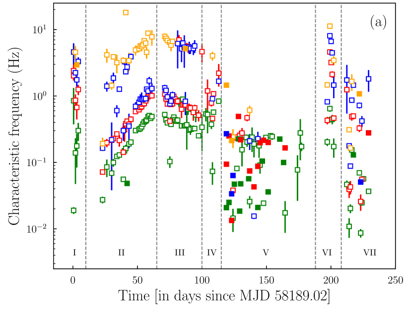
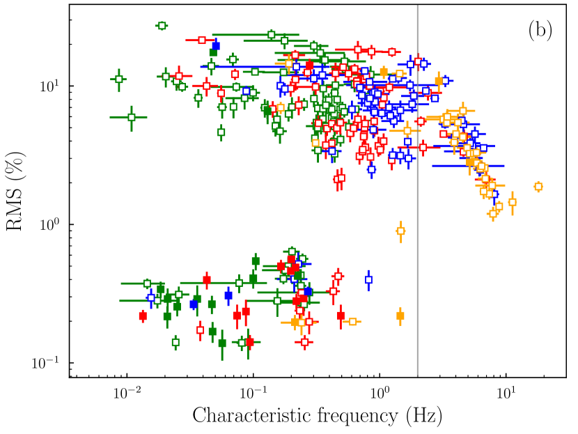
Figure 10: (a) Time evolution of the characteristic frequency ($\nu_{c}$) of different Lorentzian features corresponding to each NICER observation. First four Lorentzian of each PDS, in the increasing order of $\nu_{c}$, are indicated using green, red, blue and orange colors, respectively. Different evolutionary phases are marked from I to VII. (b) The variation of fractional RMS (in percentage) under Lorentzian with the characteristic frequency for the first four Lorentzian of NICER observations are presented with color scheme. The $\nu_{c}$ whose uncertainty can’t be estimated are shown using filled boxes.

3.5.2 RMS-Intensity Diagram (RID)

Fig. 11 shows the flux ($0.8-10$ keV) versus total fractional RMS with various evolutionary phases marked (I$-$VII). The arrow marks indicate the evolution track of the system. We can see the anti-correlation between the flux and RMS throughout this plot except in Phase-II and VII, where RMS decreases with a decrease in flux. It shares a similar pattern as in HID (Fig. 2).

At the beginning of the outburst (Phase-I), the flux is very low and the total fractional RMS is greater than 40%. The flux then increases suddenly and reaches Phase-II. In this phase, RMS decreases to 20% due to spectral softening. But the RMS increases to $\sim$ 30% in Phase-III since there is no spectral softening due to the reduction in thermal flux. The spectral state transition to HSS (Phase-V) takes place very fast and RMS drops to the lowest possible value. The flux declines gradually (Phase-V) and the source has a low RMS ($<1\%$) in this state. The flux then decreases in a faster way (Phase-VI) and reaches the quiescent state (VII) as the outburst ends. At the same time, RMS increases quickly and reaches back to the same level as in Phase-I.

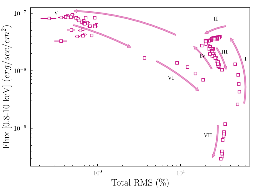
Figure 11: RID, the flux versus total RMS (in percentage) is presented with various phases identified as in Fig. 1 to understand the trend of evolution.

3.5.3 Hardness-RMS Diagram (HRD)

Total fractional RMS versus hardness (Hardness-RMS diagram) is shown in Fig. 12. This figure represents an overall combination of the spectral and temporal characteristics. The evolutionary track is marked from I to VII as before.

The outburst starts (Phase-I) with a high value of hardness and the total fractional RMS $>40\%$ but as it proceeds, hardness decreases along with the RMS, and the source enters into Phase-II where RMS decreases to 20%. Here, both are correlated due to spectral softening. Then RMS increases slightly in Phase-III with a very little change in hardness. Outburst-I ends here spanning almost a linear region with higher values of HR and RMS. During HSS (Phase-V), there is significant variation in the hardness with approximate constant ($<1\%$) RMS. Phase-VI possibly shows a state transition in the intermediate state as there are significant variations in both HR and RMS but no high frequency variability in the light curve is observed to confirm it. Finally, the source moves back to the quiescence with high HR and RMS. The Outburst-II spans a wider parameter space in HRD and completes a figure 8-shaped hysteresis loop.

Figure 12: Hardness-RMS diagram (HRD) for the NICER observations. Total fractional RMS corresponds to the frequency range $0.02-40$ Hz in the full energy range is plotted against hardness.

4 A Possible Accretion Scenario

We attempt to understand the accretion scenario of MAXI J1820+070 during the 2018 outburst using standard accretion disk (Shakura & Sunyaev, 1973) picture. We find from the spectral modelling of NICER data (Fig. 3b) that the minimum value of diskbb norm is, $N_{d}\sim 1.5\times 10^{4}$ during the HSS of Outburst-II. The corresponding inner disk radius of the diskbb model is $r_{in}=D\sqrt{N_{d}/cos(\theta)}$, where, $D$ is the distance to the source in 10 kpc, $\theta$ is the inclination of the system in degree and $r_{in}$ is in km. Given $\theta=63^{\circ}$ and $D=2.96$ kpc (Atri et al., 2020), $r_{in}=122$ km and it is consistent with the true inner radius $R_{in}\sim R_{ISCO}=0.44\,\kappa^{2}\,r_{in}$ (Kubota et al., 1998) of a Schwarzschild BH of mass $8.5M_{\odot}$ (Torres et al., 2020) with $\kappa=1.7$. This shows that the accretion disk has reached close to the innermost stable circular orbit (ISCO) during the HSS of Outburst-II. Outburst-I starts with low $T_{in}\sim 0.15$ keV (Fig. 3a) and $N_{d}\sim 1.6\times 10^{4}$ (Fig. 3b). The flux reaches the peak just in 10 days. Notice that $N_{d}$ is very similar to the value during the HSS and hence $R_{in}$ is close to the ISCO. Therefore, both outbursts start close to the central object and are having shorter rise time.

The generally accepted disk instability model (Osaki, 1974; van Paradijs & McClintock, 1994; Lasota, 2001) suggests that an outburst can be triggered due to the thermal-viscous instability when the temperature of the disk crosses the hydrogen ionization temperature. The instability raises the temperature of the disk forming a hot propagating ionizing front which enhances the accretion of matter. Outburst can be triggered either at the outer part of the accretion disk (outside-in) or the inner part (inside-out). Since the accretion happens at the viscous timescale, the outside-in trigger will have a longer rise time ($\sim 50-100$ days) whereas inside-out trigger produces an outburst of shorter rise time ($\sim 10-20$ days). Most of the outbursts of GX 339-4 are examples of the former category (Aneesha et al., 2019) whereas that of GRO J1655-40 and H1743-322 belong to the second class (Aneesha & Mandal, 2020) of outbursts.

The short rise time and low $R_{in}$ is consistent with an inside-out triggering for MAXI J1820+070. Therefore, the hot ionizing front moves outward pushing the disk outward ($N_{d}$ increases sharply, Fig. 3b) with an enhancement of $T_{in}$ (Fig. 3a) due to a surge in accretion rate, $\dot{m}$, ($T_{in}\propto\dot{m}^{1/4}r^{-3/4}_{in}$). During the decay phase (Phase-II, III), the accretion rate continues to decline with a very slow inward movement of the disk keeping the disk temperature approximately constant. The disk is truncated in the range $13-18r_{g}$ and the similar conclusion is drawn by Zdziarski et al. (2021a) using Insight-HXMT, NuSTAR and INTEGRAL data.

At around $\sim$ 100 days (Phase-IV), one more inside-out triggering (Outburst-II) takes place and the next 20 days it is a repetition of the rising phase of Outburst-I. But the difference is that Outburst-I has been triggered from quiescence (low $T_{in}$) whereas the second triggering has happened when the disk is sufficiently hot ($T_{in}=0.28$ keV). Therefore, the accretion process is more dramatic, particularly in the last 5 days of the rising phase. The disk becomes so hot ($T_{in}$ increase by a factor of 2.6) that the viscous timescale reduces and the $R_{in}$ reaches (reduce by a factor of 3.5) close to $R_{ISCO}$ in just 5 days. The soft flux under the diskbb component at the peak of Outburst-II is $5\times 10^{-8}$ erg/cm²/s and it corresponds to a luminosity of $5.3\times 10^{37}$ erg/s for an assumed distance of $2.96$ kpc (Atri et al., 2020). It means the source is accreting only at the $5\%$ of its Eddington accretion rate ($\dot{M}_{Edd}=$ $1.2\times 10^{19}$ gm/s) with an assumed mass of $8.5M_{\odot}$ (Torres et al., 2020) and 10% accretion efficiency. Even though the source is having a low accretion rate, the system appears to be very bright due to proximity and low column density along the line of sight. A low luminosity outburst is expected for an inside-out triggering due to the limited size of the disk in the hot state (Lasota, 2001). The source continues to be in HSS with approximately no change in $R_{in}$, whereas $T_{in}$ continues to decrease due to the decline of the accretion rate. Finally, the disk becomes cooler once the accretion of hot matter is over and the source reaches the quiescence.

The broadband spectral study using reflection modelling (§3.4.2) reveals the presence of a dynamical corona in the LHS (Phase-II and Phase-III), while the inner disk remains truncated and evolves marginally. Therefore, the evolution of spectral and timing properties in this state are regulated by the dynamical evolution of the corona. Fig. 10a shows that the characteristic frequency of QPOs, $\nu_{c}$, increases with time in Phase-II whereas it decreases with time in Phase-III. Among the few possible physical scenarios for the origin of LFQPOs, Stella et al. (1999); Motta et al. (2018) and Ingram & Motta (2019) proposed Lense-Thirring precession of inner accretion can be an effective mechanism. Lense-Thirring precession mechanism required a misalignment of $\gtrsim 5^{\circ}$ between the BH spin axis and the binary orbital plane (Ingram & Motta, 2019; Miller-Jones et al., 2019). Poutanen et al. (2021) recently reported that there is a misalignment of at least $40^{\circ}$ between the black hole spin and the orbital angular momentum for MAXI J1820+070. Also, the inner radius of the disk needs to be dynamic to produce the QPO evolution with time. That means $R_{in}$ has to move inward and outward during Phase-II and Phase-III, respectively. However, we understand from the spectral modelling (§3.1 and §3.4) that the $R_{in}$ decreases marginally ($R_{in}\sim 13-18r_{g}$) during the LHS (Phase-II and III). Done et al. (2007) suggested that $R_{in}$ derived from diskbb norm using simple spectral models such as $diskbb+powerlaw$ may not always be reliable. However, there are other studies in the literature that support the truncated disk geometry and dynamic corona in the LHS of this source. For example, Kara et al. (2019) and Wang et al. (2020) used reverberation time lags between the emission from the corona and the irradiated accretion disk, and suggested a contracting corona in the LHS rather than a changing inner radius of the accretion disk. Buisson et al. (2019) and You et al. (2021) also arrived at the similar conclusion using reflection modelling of the NuSTAR data. Similarly, Zdziarski et al. (2021a) performed reflection modelling of HXMT, NuSTAR and INTEGRAL data and suggested $R_{in}>10r_{g}$ in the LHS. Also, Zdziarski et al. (2021b) supported the presence of a truncated disk using thermal Comptonization and reflection modelling of NuSTAR and INTEGRAL data. Therefore, Lense-Thirring precession of inner accretion flow cannot explain the evolution of QPO frequency of the source completely.

However, the other competing picture for the origin of LFQPO is the propagation of shock oscillation model (Molteni et al., 1996; Chakrabarti et al., 2004, and reference therein). Here, oscillation of the ‘hot’ corona due to the resonance between the cooling timescale and the local dynamical timescale can produce LFQPOs. During Phase-II, the supply of soft photons remain steady as the disk is not evolving and therefore, the photon number in the corona is approximately constant (powerlaw norm remains constant, Fig. 4b). The soft photons are going to cool the electrons in the corona and a slow but steady spectral softening takes place. It reduces the cooling timescale of electrons in the corona. If the LFQPOs are produced due to the resonance between the cooling timescale and the local dynamical timescale, the QPO frequency will increase with time. On the other hand, in Phase-III, the number of thermal photons decreases gradually which increases the cooling timescale and hence a reverse evolution is observed. Note that in Phase-II, the inverse-Comptonization of soft photons in the ‘hot’ corona is significantly high as the soft photon source remains steady. The hard photons lag behind the soft photons due to inverse-Comptonization effect. The reflection modelling (Fig. 8a) shows that the corona is dynamic and moving closer to the central source in Phase-II. It means that the size of the corona becomes smaller and optical depth decreases in this phase. In an optically thin medium, the inverse-Compton spectral index is $\alpha=-$ln $\tau/$ ln $A$ (Rybicki & Lightman, 1979), where $\tau$ is the optical depth and $A$ is the mean amplification factor per scattering. The decrease of optical depth or/and reduction of amplification factor due to cooling can cause spectral softening observed in Phase-II. In the former case, considering $A$ to be constant, the number of scatterings required to produce a high energy photon remain constant, and the soft photon stays longer inside the corona due to an increase in the mean free path. In the second case, assuming a constant mean free path, the number of scatterings required to produce a high energy photon increase as $A$ reduces, and the soft photon spends a longer time inside the corona. The physical situation is possibly a combination of both effects mentioned above. Therefore, spectral softening is associated with the increase of hard lag in Phase-II, as Wang et al. (2020) reported. However, in Phase-III, the soft photons flux decreases gradually, spectra become slightly harder due to a reduction of cooling and the hard lag decreases (Wang et al., 2020). Also, we have seen in Phase-II, the size of the corona decreases (Fig. 8a) as the local dynamical timescale decreases and a reverse trend is expected in Phase-III. However, two closely spaced simultaneous data points in phase-III (Fig.  8a) are not sufficient to comment if corona moves outward.

The geometry of the corona is generally described either as vertically elongated (Martocchia & Matt, 1996; Uttley et al., 2014; Niedźwiecki et al., 2016) or radially extended (Chakrabarti & Titarchuk, 1995; Wilkins & Gallo, 2015; Poutanen et al., 2018). We understand that the reflection modelling of the broadband spectral data supports a vertically elongated corona. In contrast, the evolution of LFQPO caused by the propagation of the shock oscillation model suggests a radially extended corona inside the truncated disk. The comprehensive spectral and timing studies suggest a complex geometry of the corona (Fürst et al., 2015; Niedźwiecki et al., 2016; Wilkins et al., 2016; Gonzalez et al., 2017; Zoghbi et al., 2020) in the LHS of the source. It demands further investigation of the coronal geometry, which is beyond the scope of the present work.

5 Summary and Conclusion

We have performed spectral analysis of NICER and Swift/XRT data (§3.1) independently during Outburst-I and Outburst-II. The NICER and XRT light curve is shown in Fig. 1, which has two successive outbursts during this period. The Outburst-I is dominated by the non-thermal photons (peak flux in $2-10$ keV is 2.4 times the same in $0.8-2$ keV) whereas the Outburst-II is very bright and soft. The same trend is found in $10-60$ keV (filled star in Fig. 1) from simultaneous broadband spectral modelling. The HID with different spectral states is presented in Fig. 2. The Outburst-I is evolved only in the LHS and classified as a ‘failed’ outburst, whereas the Outburst-II shows a transition from LHS to HSS via a very brief intermediate state. There is an overall offset ($\sim$ 22%) in the HR between XRT and NICER due to difference in the spectral responses (discussed in Appendix-A). We have done broadband spectral modelling of all available simultaneous data of NICER-NuSTAR, XRT-NuSTAR and AstroSat (SXT-LAXPC) to understand the presence of various model components (§3.4.1) in the spectra. Also, the broadband reflection modelling (§3.4.2) shows the presence of strong reflection signature during both outbursts and presence of an evolving corona in the LHS. The timing analysis shows the presence of multiple QPO-like features and we have studied the time evolution of their characteristic frequency (Fig. 10a). The RMS under the Lorentzian features in the PDS indicates an interesting correlation. We find a clear anti-correlation between the fractional RMS and $\nu_{c}$ (Fig. 10b) for $\nu_{c}>2$ Hz. This is a signature of type-C QPO and is commonly observed in LHS (Belloni, 2010; Athulya et al., 2022). However, no clear correlation is observed at the lower frequency. Below, we summarise the important findings of this work combining the spectral and timing studies during various phases of evolution of the source.

• Phase-I (Rising phase, Outburst-I)
  Fig. 3 and Fig. 4 show that both thermal and non-thermal flux increases in the rising phase with an increase of $T_{in}$ and powerlaw norm with a hard spectrum ($\Gamma\sim 1.5$). The NICER and NuSTAR data show the presence of Fe $K_{\alpha}$ line (Fig. 5 and Epoch 1 in Table 3) and the presence of significant reflection. The lamp-post height is significantly large ($\sim 200r_{g}$) with a high ionization parameter ($log$ $\xi=2.01^{+0.08}_{-0.06}$) and iron abundance $A_{Fe}=2.4\pm 0.1$. PDS shows the presence of QPO-like features in $0.1-5$ Hz (Fig. 10a) and the fractional RMS $\sim 40\%$ (Fig 11).
  

• Phase-II
  In this phase, the thermal disk component is very steady with $T_{in}\sim 0.27$ keV (Fig. 3a) and $R_{in}$ evolves very little ($15-18r_{g}$). The non-thermal photon flux also remains steady with the gradual spectral softening (Fig. 4a). We observe reflection signature of Fe $K_{\alpha}$ line (Fig. 5) with an increasing trend in the line energy and absorption edge (Epoch $2-5$ in Table 3). The reflection modelling (Epoch $2-5$ in Table 4) of broadband data shows a gradual decrease of lamp-post height to $\sim 30r_{g}$ with an enhancement in the reflection fraction $R_{f}\sim 0.6$. The disk iron abundance remains similar to the rising phase but there is a reduction in the ionization parameter ($log$ $\xi\sim 1.7$). The timing results show that the characteristic frequency ($\nu_{c}$) increases with time from $\sim 0.1$ to $10$ Hz (Fig. 10a) as the flux decreases. This is generally not observed in outbursting sources. As we have discussed in §4, one possible reason could be the spectral softening due to the reduction of cooling timescale of electrons in the corona as the thermal component remains steady. And the resonance oscillation between cooling timescale and dynamical timescale produces the LFQPOs (Molteni et al., 1996; Chakrabarti et al., 2004). The spectral softening leads to a correlated reduction of the fractional RMS (Phase-II in Fig. 11) with the observed flux. The RMS lies in $30-20\%$ range with a reduction in HR in this phase (Fig. 12).
  

• Phase-III
  A steady decrease in the thermal and non-thermal components of flux is observed in this phase of the outburst. A steady decrease in $T_{in}$ (Fig. 3a) and powerlaw norm (Fig. 4b) is observed without any spectral softening ($\Gamma\sim 1.7$). The NICER data possess reflection signature of Fe $K_{\alpha}$ line (Fig. 5). The wideband spectral study shows the presence of Fe absorption edge (Epoch 6-7 in Table 3). The reflection parameters (Fig. 8) are similar to the previous phase. We observed that the characteristic frequencies ($\nu_{c}$) in the PDS decreases (Fig. 10a) with time. The total fractional RMS increases with the decrease in flux (Phase-III in Fig. 11) which is consistent with the general characteristic in the LHS. This is due to the overall decrease in the number of photons in corona and it becomes difficult to cool the corona further. The RMS increases to 30% with almost constant HR (Fig. 12) since both thermal and non-thermal flux decrease in a similar manner.

  After this, the source moves to Outburst-II through a rising phase (Phase-IV) similar to the Outburst-I. The simultaneous broadband data show reflection signature (Fig. 8) with similar parameter as in Phase-II. The characteristic frequency, $\nu_{c}$, increases with time (Fig. 10a) as flux increases. Both fractional RMS and HR reduce and the source moves to HSS very fast.
  

• Phase-V (HSS, Outburst-II)
  The spectrum in this state is dominated by the thermal emission flux. The disk moves close to the inner edge with $T_{in}\sim 0.7$ keV (Fig. 3a) and spectrum becomes very soft, $\Gamma>3.0$ (Fig. 4a), though simultaneous spectral modelling (Epoch 9-12) in Table 3 and Table 4 provide relatively lower index. The NICER data do not show any Fe line signature though simultaneous broadband data show high reflection fraction $R_{f}\sim 3.5$, high ionization parameter ($log$ $\xi\sim 4$), and over-abundance of iron. The timing properties show featureless PDS with very low RMS (Phase-V in Fig. 11) and HR varies between $\sim 0.5-0.7$ (Fig. 12).
  

• Phase-VI & VII (Decay towards quiescence)
  The light curve in the decline phase of Outburst-II is initially linear and becomes exponential towards the end. $T_{in}$ decreases (Fig. 3a), $R_{in}$ gradually move outward and the spectrum becomes harder (Fig. 4a). The reflection modelling (Fig. 8) shows that the reflection fraction and the lamp-post height decrease gradually. Fig. 10a shows that $\nu_{c}$ increases at the end of HSS and decreases with the declination of the flux. The spectro-temporal properties indicate that this phase passes through the intermediate state (Phase-VI in Fig. 12) with a fractional RMS of 10% and HR $\sim 1$. At the end, the source returns back to LHS (Phase- VII in Fig. 12) with RMS $\sim$ 30% and HR $\sim 3$.

Finally, we discuss the possible accretion scenario during the 2018 outburst in §4. We propose that both outbursts are triggered as inside-out propagation of thermo-viscous instability which produces outbursts with a short rise time. The spectral modelling shows that the Outburst-I has been triggered close to the inner edge and the disk remains truncated during Outburst-I. The rise of flux in Outburst-II is dramatic since the outburst triggering has happened when the disc is sufficiently hot and the viscous timescale becomes short enough that the inner disk moves close to ISCO very fast and produce bright HSS. The accretion disk remains truncated ($\sim 10$ $r_{g}$) once the source reaches the quiescence. The comprehensive spectral and timing studies reveal that a lamp-post corona or a radially extended corona is inadequate to interpret the observed data. The results suggest a complex corona geometry in the LHS of MAXI J1820+070. The outcome of this study challenges the present understanding of coronal geometry and suggests further investigation of disk-jet geometry around black holes.

Data Availability

The data from Swift/XRT, NICER and NuSTAR underlying this article are available in HEASARC, at https://heasarc.gsfc.nasa.gov/docs/archive.html. AstroSat data archive is available at https://astrobrowse.issdc.gov.in/astro_archive/archive/Home.jsp.

Appendix A XRT and NICER Spectral Discrepancies

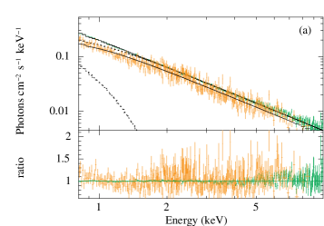
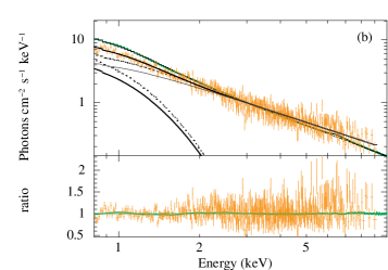
Figure 13: (a) Simultaneous XRT and NICER spectrum on MJD 58212 fitted using tbabs(diskbb+po) for XRT and tbabs(diskbb+gauss+po) for NICER, and are plotted together. The orange color corresponds to the XRT and green is for NICER. (b) Quasi-simultaneous observation on $\sim$ MJD 58401 are fitted using tbabs*po and tbabs(diskbb+po) for XRT and NICER respectively with the same color scheme.

The estimation of spectral parameters gets affected due to the difference in spectral energy resolution of XRT and NICER. To understand it better, we model two pairs of simultaneous NICER and XRT observations, the first one is on MJD 58212 (Pair-I) and the second observation (Pair-II) is on $\sim$ MJD 58401 (Pair-II is a quasi-simultaneous, but the source did not evolve significantly during the observations).

Pair-I observation is close to the peak of Outburst-I and the model tbabs(diskbb+po) provides a good fitting for XRT data whereas NICER data need an additional Gaussian component due to Fe $K_{\alpha}$ emission line signature. The fitted spectra for both XRT and NICER data are plotted together in Fig. 13a. Here, the orange color represents the XRT spectrum and green color represents NICER spectrum. Pair-II observation is close to the quiescence after Outburst-II. The tbabs(diskbb+po) model is needed to fit the NICER data but only a powerlaw component (tbabs $\times$ po) is enough to fit the XRT data and the model fitting is presented in Fig. 13b. For a given simultaneous observation, the requirement of additional model components for NICER data imply that the NICER calibration is still updating since Swift/XRT is well calibrated with other instruments (Madsen et al., 2017).

We attempt an order of magnitude estimation of the spectral discrepancies between the instruments from these simultaneous observations. The model fitted parameters and estimated fluxes in various energy bands are summarised in Table 5. We find that the overall ($0.8-10$ keV) flux matches well when the source was bright (Pair-I) though NICER flux in the high energy ($2-10$ keV) band is 7.1% lower than the XRT flux due to a steeper spectral index (difference of $\sim$ 0.24). However, the inner disk temperature, $T_{in}$ is comparable but a higher diskbb norm reflects 5.8% higher flux in low energy ($0.8-2$ keV) band. Therefore, there is a mutual balance between the low and high energy fluxes, keeping the overall fluxes comparable when the source is bright. Note that the XRT flux in $0.8-10$ keV band is used as a reference to calculate the percentage of flux difference. The spectral index for Pair-II data set appears comparable. But a higher powerlaw norm and the presence of additional disk components record 13.6% and 7.3% higher flux in the high and low energy band respectively for NICER. Therefore, we find considerable amount of discrepancies between fluxes in the high and low energy bands due to the differences in spectral response.

Finally, the simultaneous multi-mission observation campaign of quasar 3C 273 involving NuSTAR, Swift, and NICER were performed on 2019-07-02, 2020-07-06, and 2021-06-09. The recent report (Madsen et al., 2021) of International Astronomical Consortium for High Energy Calibration (IACHEC) has mentioned that the data analysis of these observations is underway. Therefore, the NICER calibration is still evolving and a proper NICER-Swift/XRT cross-calibration is very much required.

Table 5: Model fitted parameters and estimated fluxes in various energy bands from simultaneous NICER-XRT fittings

Model	Component	Pair I		Pair II
		NICER	XRT	NICER	XRT
powerlaw	$\Gamma$	$1.648_{-0.004}^{+0.004}$	$1.41_{-0.07}^{+0.07}$	$1.70_{-0.01}^{+0.01}$	$1.69_{-0.03}^{+0.03}$
	norm	$6.16_{-0.04}^{+0.04}$	$4.68_{-0.05}^{+0.05}$	$0.214_{-0.003}^{+0.003}$	$0.179_{-0.004}^{+0.004}$
diskbb	$T_{in}(keV)$	$0.283_{-0.004}^{+0.004}$	$0.30_{-0.03}^{+0.04}$	$0.18_{-0.01}^{+0.01}$	-
	norm ($\times 10^{4}$)	$11.1_{-0.63}^{+0.68}$	$6.78_{-2.4}^{+4.7}$	$1.43_{-0.47}^{+0.78}$	-
gauss	line E (keV)	$6.60_{-0.04}^{+0.04}$	-	-	-
	sigma (keV)	0.6†	-	-	-
	norm	$0.034_{-0.002}^{+0.002}$	-	-	-
$\chi^{2}_{red}$		1.02	1.16	1.04	0.86
Flux (ergs/sec/cm2)	Energy range	$(\times 10^{-8})$	$(\times 10^{-8})$	$(\times 10^{-9})$	$(\times 10^{-9})$
	0.8-10 keV	$3.945_{-0.002}^{+0.002}$	$4.00_{-0.06}^{+0.03}$	$1.189_{-0.007}^{+0.004}$	$0.98_{-0.01}^{+0.01}$
	0.8-2 keV	$1.180_{-0.002}^{+0.001}$	$0.948_{-0.020}^{+0.003}$	$0.314_{-0.003}^{+0.007}$	$0.242_{-0.003}^{+0.002}$
	2-10 keV	$2.765_{-0.002}^{+0.002}$	$3.05_{-0.04}^{+0.06}$	$0.874_{-0.005}^{+0.005}$	$0.74_{-0.01}^{+0.01}$

• $\dagger$ frozen parameter.

References

- Agrawal (2006) Agrawal P. C., 2006, Advances in Space Research, 38, 2989
- Agrawal et al. (2018) Agrawal V. K., Nandi A., Girish V., Ramadevi M. C., 2018, MNRAS, 477, 5437
- Alam et al. (2014) Alam M. S., Dewangan G. C., Belloni T., Mukherjee D., Jhingan S., 2014, MNRAS, 445, 4259
- Aneesha & Mandal (2020) Aneesha U., Mandal S., 2020, A&A, 637, A47
- Aneesha et al. (2019) Aneesha U., Mandal S., Sreehari H., 2019, MNRAS, 486, 2705
- Antia et al. (2017) Antia H. M., et al., 2017, ApJS, 231, 10
- Antia et al. (2021) Antia H. M., et al., 2021, Journal of Astrophysics and Astronomy, 42, 32
- Athulya et al. (2022) Athulya M. P., Radhika D., Agrawal V. K., Ravishankar B. T., Naik S., Mandal S., Nandi A., 2022, MNRAS, 510, 3019
- Atri et al. (2020) Atri P., et al., 2020, MNRAS, 493, L81
- Axelsson & Veledina (2021) Axelsson M., Veledina A., 2021, MNRAS, 507, 2744
- Baby et al. (2020) Baby B. E., Agrawal V. K., Ramadevi M. C., Katoch T., Antia H. M., Mandal S., Nandi A., 2020, MNRAS, 497, 1197
- Bambi et al. (2021) Bambi C., et al., 2021, Space Sci. Rev., 217, 65
- Belloni (2005) Belloni T., 2005, in Burderi L., Antonelli L. A., D’Antona F., di Salvo T., Israel G. L., Piersanti L., Tornambè A., Straniero O., eds, American Institute of Physics Conference Series Vol. 797, Interacting Binaries: Accretion, Evolution, and Outcomes. pp 197–204 (arXiv:astro-ph/0504185), doi:10.1063/1.2130233
- Belloni (2010) Belloni T. M., 2010, States and Transitions in Black Hole Binaries. p. 53, doi:10.1007/978-3-540-76937-8_3
- Belloni et al. (2005) Belloni T., Homan J., Casella P., van der Klis M., Nespoli E., Lewin W. H. G., Miller J. M., Méndez M., 2005, A&A, 440, 207
- Bharali et al. (2019) Bharali P., Chauhan J., Boruah K., 2019, MNRAS, 487, 5946
- Bhargava et al. (2021) Bhargava Y., Belloni T., Bhattacharya D., Motta S., Ponti. G., 2021, MNRAS, 508, 3104
- Bright et al. (2018) Bright J., Motta S., Fender R., 2018, The Astronomer’s Telegram, 12061, 1
- Buisson et al. (2018) Buisson D., Fabian A., Alston W., Walton D., Kara E., Garcia J., Homan J., Tomsick J., 2018, The Astronomer’s Telegram, 11578, 1
- Buisson et al. (2019) Buisson D. J. K., et al., 2019, MNRAS, 490, 1350
- Buisson et al. (2021) Buisson D. J. K., et al., 2021, MNRAS, 500, 3976
- Casella et al. (2005) Casella P., Belloni T., Stella L., 2005, ApJ, 629, 403
- Chakrabarti & Titarchuk (1995) Chakrabarti S., Titarchuk L. G., 1995, ApJ, 455, 623
- Chakrabarti et al. (2004) Chakrabarti S. K., Acharyya K., Molteni D., 2004, A&A, 421, 1
- Chakraborty et al. (2020) Chakraborty S., Navale N., Ratheesh A., Bhattacharyya S., 2020, MNRAS, 498, 5873
- Corral-Santana et al. (2016) Corral-Santana J. M., Casares J., Muñoz-Darias T., Bauer F. E., Martínez-Pais I. G., Russell D. M., 2016, A&A, 587, A61
- Cunningham (1975) Cunningham C. T., 1975, ApJ, 202, 788
- Dauser et al. (2013) Dauser T., Garcia J., Wilms J., Böck M., Brenneman L. W., Falanga M., Fukumura K., Reynolds C. S., 2013, MNRAS, 430, 1694
- Dauser et al. (2014) Dauser T., Garcia J., Parker M. L., Fabian A. C., Wilms J., 2014, MNRAS, 444, L100
- Dauser et al. (2016) Dauser T., García J., Walton D. J., Eikmann W., Kallman T., McClintock J., Wilms J., 2016, A&A, 590, A76
- De Marco et al. (2021) De Marco B., Zdziarski A. A., Ponti G., Migliori G., Belloni T. M., Segovia Otero A., Dziełak M. A., Lai E. V., 2021, A&A, 654, A14
- Denisenko (2018) Denisenko D., 2018, The Astronomer’s Telegram, 11400, 1
- Done et al. (2007) Done C., Gierliński M., Kubota A., 2007, A&ARv, 15, 1
- Dziełak et al. (2021) Dziełak M. A., De Marco B., Zdziarski A. A., 2021, MNRAS, 506, 2020
- Fabian et al. (2000) Fabian A. C., Iwasawa K., Reynolds C. S., Young A. J., 2000, PASP, 112, 1145
- Fabian et al. (2020) Fabian A. C., et al., 2020, MNRAS, 493, 5389
- Fender et al. (2004) Fender R. P., Belloni T. M., Gallo E., 2004, MNRAS, 355, 1105
- Fiori et al. (2018) Fiori M., et al., 2018, The Astronomer’s Telegram, 11824, 1
- Fürst et al. (2015) Fürst F., et al., 2015, ApJ, 808, 122
- García et al. (2014) García J., et al., 2014, ApJ, 782, 76
- García et al. (2016) García J. A., Fabian A. C., Kallman T. R., Dauser T., Parker M. L., McClintock J. E., Steiner J. F., Wilms J., 2016, MNRAS, 462, 751
- Gonzalez et al. (2017) Gonzalez A. G., Wilkins D. R., Gallo L. C., 2017, MNRAS, 472, 1932
- Guan et al. (2021) Guan J., et al., 2021, MNRAS, 504, 2168
- Harrison et al. (2013) Harrison F. A., et al., 2013, ApJ, 770, 103
- Homan & Belloni (2005) Homan J., Belloni T., 2005, Ap&SS, 300, 107
- Homan et al. (2001) Homan J., Wijnands R., van der Klis M., Belloni T., van Paradijs J., Klein-Wolt M., Fender R., Méndez M., 2001, ApJS, 132, 377
- Homan et al. (2020) Homan J., et al., 2020, ApJ, 891, L29
- Ingram & Motta (2019) Ingram A. R., Motta S. E., 2019, New Astron. Rev., 85, 101524
- Iyer et al. (2015) Iyer N., Nandi A., Mandal S., 2015, ApJ, 807, 108
- Kara et al. (2019) Kara E., et al., 2019, Nature, 565, 198
- Katoch et al. (2021) Katoch T., Baby B. E., Nandi A., Agrawal V. K., Antia H. M., Mukerjee K., 2021, MNRAS, 501, 6123
- Kawamura et al. (2022) Kawamura T., Axelsson M., Done C., Takahashi T., 2022, MNRAS,
- Kawamuro et al. (2018) Kawamuro T., et al., 2018, The Astronomer’s Telegram, 11399, 1
- Kubota et al. (1998) Kubota A., Tanaka Y., Makishima K., Ueda Y., Dotani T., Inoue H., Yamaoka K., 1998, PASJ, 50, 667
- Lasota (2001) Lasota J.-P., 2001, New Astron. Rev., 45, 449
- Lightman & White (1988) Lightman A. P., White T. R., 1988, ApJ, 335, 57
- Ma et al. (2021) Ma X., et al., 2021, Nature Astronomy, 5, 94
- Madsen et al. (2017) Madsen K. K., Beardmore A. P., Forster K., Guainazzi M., Marshall H. L., Miller E. D., Page K. L., Stuhlinger M., 2017, AJ, 153, 2
- Madsen et al. (2021) Madsen K. K., et al., 2021, arXiv e-prints, p. arXiv:2111.01613
- Malzac et al. (2006) Malzac J., et al., 2006, A&A, 448, 1125
- Marino et al. (2021) Marino A., et al., 2021, A&A, 656, A63
- Martocchia & Matt (1996) Martocchia A., Matt G., 1996, MNRAS, 282, L53
- Mastroserio et al. (2021) Mastroserio G., et al., 2021, MNRAS, 507, 55
- Mereminskiy et al. (2018) Mereminskiy I. A., Grebenev S. A., Molkov S. V., Zaznobin I. A., Khorunzhev G. A., Burenin R. A., Eselevich M. V., 2018, The Astronomer’s Telegram, 11488, 1
- Miller-Jones et al. (2019) Miller-Jones J. C. A., et al., 2019, Nature, 569, 374
- Mitsuda et al. (1984) Mitsuda K., et al., 1984, PASJ, 36, 741
- Molteni et al. (1996) Molteni D., Sponholz H., Chakrabarti S. K., 1996, ApJ, 457, 805
- Morgan et al. (1997) Morgan E. H., Remillard R. A., Greiner J., 1997, ApJ, 482, 993
- Motta et al. (2011) Motta S., Muñoz-Darias T., Casella P., Belloni T., Homan J., 2011, MNRAS, 418, 2292
- Motta et al. (2012) Motta S., Homan J., Muñoz Darias T., Casella P., Belloni T. M., Hiemstra B., Méndez M., 2012, MNRAS, 427, 595
- Motta et al. (2018) Motta S. E., Franchini A., Lodato G., Mastroserio G., 2018, MNRAS, 473, 431
- Muñoz-Darias et al. (2019) Muñoz-Darias T., et al., 2019, ApJ, 879, L4
- Mudambi et al. (2020) Mudambi S. P., Maqbool B., Misra R., Hebbar S., Yadav J. S., Gudennavar S. B., S. G. B., 2020, ApJ, 889, L17
- Mushotzky et al. (1993) Mushotzky R. F., Done C., Pounds K. A., 1993, ARA&A, 31, 717
- Nandi et al. (2012) Nandi A., Debnath D., Mandal S., Chakrabarti S. K., 2012, A&A, 542, A56
- Narayan & Yi (1995) Narayan R., Yi I., 1995, ApJ, 452, 710
- Niedźwiecki et al. (2016) Niedźwiecki A., Zdziarski A. A., Szanecki M., 2016, ApJ, 821, L1
- Osaki (1974) Osaki Y., 1974, PASJ, 26, 429
- Paice et al. (2019) Paice J. A., et al., 2019, MNRAS, 490, L62
- Paice et al. (2021) Paice J. A., et al., 2021, MNRAS, 505, 3452
- Poutanen et al. (2018) Poutanen J., Veledina A., Zdziarski A. A., 2018, A&A, 614, A79
- Poutanen et al. (2021) Poutanen J., et al., 2021, arXiv e-prints, p. arXiv:2109.07511
- Radhika & Nandi (2014) Radhika D., Nandi A., 2014, Advances in Space Research, 54, 1678
- Radhika et al. (2016) Radhika D., Nandi A., Agrawal V. K., Mandal S., 2016, MNRAS, 462, 1834
- Remillard & McClintock (2006) Remillard R. A., McClintock J. E., 2006, ARA&A, 44, 49
- Remillard et al. (2002a) Remillard R. A., Sobczak G. J., Muno M. P., McClintock J. E., 2002a, ApJ, 564, 962
- Remillard et al. (2002b) Remillard R. A., Muno M. P., McClintock J. E., Orosz J. A., 2002b, ApJ, 580, 1030
- Remillard et al. (2021) Remillard R. A., et al., 2021, arXiv e-prints, p. arXiv:2105.09901
- Reynolds & Nowak (2003) Reynolds C. S., Nowak M. A., 2003, Phys. Rep., 377, 389
- Rodi et al. (2021) Rodi J., Tramacere A., Onori F., Bruni G., Sànchez-Fernàndez C., Fiocchi M., Natalucci L., Ubertini P., 2021, ApJ, 910, 21
- Ross & Fabian (2005) Ross R. R., Fabian A. C., 2005, MNRAS, 358, 211
- Rybicki & Lightman (1979) Rybicki G. B., Lightman A. P., 1979, Radiative processes in astrophysics. John Wiley & Sons, Inc
- Shakura & Sunyaev (1973) Shakura N. I., Sunyaev R. A., 1973, A&A, 500, 33
- Shappee et al. (2014) Shappee B. J., et al., 2014, ApJ, 788, 48
- Shidatsu et al. (2018) Shidatsu M., et al., 2018, ApJ, 868, 54
- Shidatsu et al. (2019) Shidatsu M., Nakahira S., Murata K. L., Adachi R., Kawai N., Ueda Y., Negoro H., 2019, ApJ, 874, 183
- Singh et al. (2020) Singh K. P., Stewart G., Chandra S., Dewangan G. C., Bhattacharyya S., Kamble N. S., Vishwakarma S., Koyande J. G., 2020, arXiv e-prints, p. arXiv:2012.01800
- Sreehari & Nandi (2021) Sreehari H., Nandi A., 2021, MNRAS, 502, 1334
- Sreehari et al. (2018) Sreehari H., Nandi A., Radhika D., Iyer N., Mandal S., 2018, Journal of Astrophysics and Astronomy, 39, 5
- Sreehari et al. (2019) Sreehari H., Ravishankar B. T., Iyer N., Agrawal V. K., Katoch T. B., Mandal S., Nandi A., 2019, MNRAS, 487, 928
- Stella et al. (1999) Stella L., Vietri M., Morsink S. M., 1999, ApJ, 524, L63
- Stiele & Kong (2020) Stiele H., Kong A. K. H., 2020, ApJ, 889, 142
- Sunyaev & Titarchuk (1980) Sunyaev R. A., Titarchuk L. G., 1980, A&A, 500, 167
- Sunyaev & Titarchuk (1985) Sunyaev R. A., Titarchuk L. G., 1985, A&A, 143, 374
- Tetarenko et al. (2016) Tetarenko B. E., Sivakoff G. R., Heinke C. O., Gladstone J. C., 2016, VizieR Online Data Catalog, p. J/ApJS/222/15
- Tetarenko et al. (2021) Tetarenko A. J., et al., 2021, MNRAS, 504, 3862
- Titarchuk (1994) Titarchuk L., 1994, in Fichtel C. E., Gehrels N., Norris J. P., eds, American Institute of Physics Conference Series Vol. 304, The Second Compton Symposium. pp 380–384, doi:10.1063/1.45591
- Tomsick (2018) Tomsick J., 2018, in 42nd COSPAR Scientific Assembly. pp E1.4–21–18
- Torres et al. (2019) Torres M. A. P., Casares J., Jiménez-Ibarra F., Muñoz-Darias T., Armas Padilla M., Jonker P. G., Heida M., 2019, ApJ, 882, L21
- Torres et al. (2020) Torres M. A. P., Casares J., Jiménez-Ibarra F., Álvarez-Hernández A., Muñoz-Darias T., Armas Padilla M., Jonker P. G., Heida M., 2020, ApJ, 893, L37
- Tucker et al. (2018) Tucker M. A., et al., 2018, ApJ, 867, L9
- Uttley et al. (2014) Uttley P., Cackett E. M., Fabian A. C., Kara E., Wilkins D. R., 2014, A&ARv, 22, 72
- Uttley et al. (2018) Uttley P., et al., 2018, The Astronomer’s Telegram, 11423, 1
- van Paradijs & McClintock (1994) van Paradijs J., McClintock J. E., 1994, A&A, 290, 133
- van der Klis (1989) van der Klis M., 1989, ARA&A, 27, 517
- Wang et al. (2020) Wang Y., et al., 2020, ApJ, 896, 33
- Wang et al. (2021) Wang J., et al., 2021, ApJ, 910, L3
- Wilkins & Gallo (2015) Wilkins D. R., Gallo L. C., 2015, MNRAS, 448, 703
- Wilkins et al. (2015) Wilkins D. R., Gallo L. C., Grupe D., Bonson K., Komossa S., Fabian A. C., 2015, MNRAS, 454, 4440
- Wilkins et al. (2016) Wilkins D. R., Cackett E. M., Fabian A. C., Reynolds C. S., 2016, MNRAS, 458, 200
- Wilms et al. (2000) Wilms J., Allen A., McCray R., 2000, ApJ, 542, 914
- You et al. (2021) You B., et al., 2021, Nature Communications, 12, 1025
- Yu et al. (2018) Yu W., Zhang J., Yan Z., Wang X., Bai J., 2018, The Astronomer’s Telegram, 11510, 1
- Zampieri et al. (2018) Zampieri L., Fiori M., Burtovoi A., Naletto G., Barbieri C., Ochner P., Umbriaco G., Barbieri M., 2018, The Astronomer’s Telegram, 11723, 1
- Zdziarski et al. (1994) Zdziarski A. A., Fabian A. C., Nandra K., Celotti A., Rees M. J., Done C., Coppi P. S., Madejski G. M., 1994, MNRAS, 269, L55
- Zdziarski et al. (2021a) Zdziarski A. A., You B., Szanecki M., Li X.-B., Ge M.-Y., 2021a, arXiv e-prints, p. arXiv:2112.08116
- Zdziarski et al. (2021b) Zdziarski A. A., Dziełak M. A., De Marco B., Szanecki M., Niedźwiecki A., 2021b, ApJ, 909, L9
- Zhang et al. (1995) Zhang W., Jahoda K., Swank J. H., Morgan E. H., Giles A. B., 1995, ApJ, 449, 930
- Zoghbi et al. (2020) Zoghbi A., Kalli S., Miller J. M., Mizumoto M., 2020, ApJ, 893, 97