AdaBest: Minimizing Client Drift in Federated Learning via Adaptive Bias Estimation

Abstract

In Federated Learning (FL), a number of clients or devices collaborate to train a model without sharing their data. Models are optimized locally at each client and further communicated to a central hub for aggregation. While FL is an appealing decentralized training paradigm, heterogeneity among data from different clients can cause the local optimization to drift away from the global objective. In order to estimate and therefore remove this drift, variance reduction techniques have been incorporated into FL optimization recently. However, these approaches inaccurately estimate the clients’ drift and ultimately fail to remove it properly. In this work, we propose an adaptive algorithm that accurately estimates drift across clients. In comparison to previous works, our approach necessitates less storage and communication bandwidth, as well as lower compute costs. Additionally, our proposed methodology induces stability by constraining the norm of estimates for client drift, making it more practical for large scale FL. Experimental findings demonstrate that the proposed algorithm converges significantly faster and achieves higher accuracy than the baselines across various FL benchmarks.

1 Introduction

In Federated Learning (FL), multiple sites with data often known as clients collaborate to train a model by communicating parameters through a central hub called server. At each round, the server broadcasts a set of model parameters to a number of clients. Selected clients separately optimize towards their local objective. The locally trained parameters are sent back to the server, where they are aggregated to form a new set of parameters for the next round. A well-known aggregation is to simply average the parameters received from the participating clients in each round. This method is known as FedAvg [19] or LocalSGD [27].

In order to reduce the communication costs as well as privacy concerns (for example possible leakage of data from gradients [34]), multiple local optimization steps are often preferable and sometimes inevitable [19]. Unfortunately, multiple local updates subject the parameters to client drift [9]. While SGD is an unbiased gradient descent estimator, LocalSGD is biased due to the existence of client drift. As a result, LocalSGD converges to a neighborhood around the optimal solution with a distance proportionate to the magnitude of the bias [3]. The amount of this bias itself depends on the heterogeneity among the clients’ data distribution, causing LocalSGD to perform poorly on non-iid benchmarks [33].

One effective way of reducing client drift is by adapting Reduced Variance SGD (RV-SGD) methods [8, 24, 25, 21] to LocalSGD. The general strategy is to regularize the local updates with an estimate of gradients of inaccessible training samples (i.e., data of other clients). In other words, the optimization direction of a client is modified using the estimated optimization direction of other clients. These complementary gradients could be found for each client $i$ by subtracting an estimate of the local gradients from an estimate of the oracle’s full gradients. In this paper, we refer to these two estimates with ${\bm{h}}_{i}$ and ${\bm{h}}$, respectively. Therefore, a reduced variance local gradient for client $i$ would be in general form of $\nabla L_{i}+({\bm{h}}-{\bm{h}}_{i})$ where $\nabla L_{i}$ corresponds to the true gradients of the local objective for client $i$.

The majority of existing research work on adapting RV-SGD to distributed learning do not meet the requirement to be applied to FL. Some proposed algorithms require full participation of clients [26, 23, 17]; thus, are not scalable to cross-device FL. Another group of algorithms require communicating the true gradients [16, 20] and, as a result, completely undermine the FL privacy concerns such as attacks to retrieve data from true gradients [34].

SCAFFOLD [9] is an algorithm that supports partial participation of clients and does not require the true gradients at the server. While SCAFFOLD shows superiority in performance and convergence rate compared to its baselines, it consumes twice as much bandwidth. To construct the complementary gradients, it computes and communicates ${\bm{h}}$ as an extra set of parameters to each client along with the model parameters. FedDyn [2] proposed to apply ${\bm{h}}$ in a single step prior to applying any local update, and practically found better performance and convergence speed compared to SCAFFOLD. Since applying ${\bm{h}}$ uses the same operation in all participating clients, [2] moved it to the server instead of applying on each client. This led to large savings of local computation, and more importantly to use the same amount of communication bandwidth as vanilla LocalSGD (i.e., FedAvg), which is half of what SCAFFOLD uses.

FedDyn make several assumptions that are often not satisfied in large-scale FL. These assumptions include having prior knowledge about the total number of clients, a high rate of re-sampling clients, and drawing clients uniformly from a stationary set. Even with these assumptions, we show that ${\bm{h}}$ in FedDyn is pruned to explosion, especially in large-scale setting. This hurts the performance and holds the optimization back from converging to a stationary point.

Figure 1: Asymptotic instability of FedDyn as a results of unbounded increase of $\|{\bm{h}}^{t}\|$. From top to bottom test loss (log scale), norm of cloud parameters, and test accuracy are shown in subplots. The shared horizontal axis shows the number of communication rounds. Each experiment is repeated 5 times with different random seed of data partitioning. Solid lines and shades represent mean and standard deviation respectively

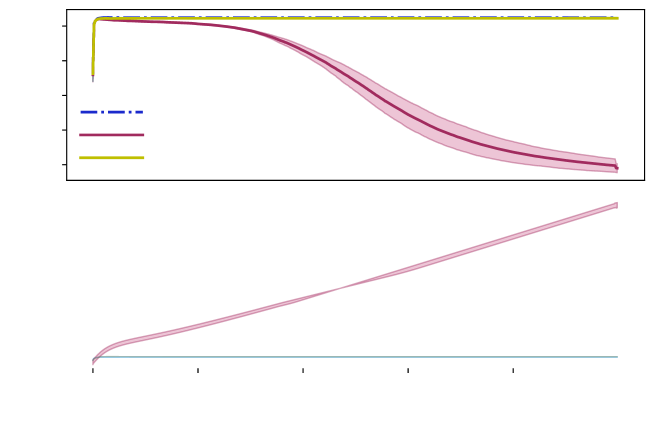
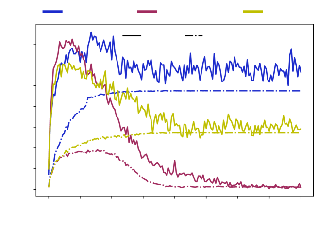
This paper proposes AdaBest, a Reduced Variance LocalSGD (RV-LSGD) solution to minimize the client drift in FL. Compared to the baselines, we define a simpler yet more elegant method of incorporating previous observations into estimates of complementary gradients. Our solution alleviates the instability of the norm of ${\bm{h}}$ in FedDyn (see Figure 1 for empirical evaluation) while consuming the same order of storage and communication bandwidth, and even reducing the compute cost (see supplementary material for quantitative comparison). Unlike previous works, our algorithm provides a mechanism for adapting to changes in the distribution of client sampling and does not require prior knowledge of the entire set of clients. These characteristics of AdaBest, combined with its stability, provide a practical solution for large-scale cross-device FL. Our main contributions are as follows:

• We show that the existing RV-LSGD approaches for cross-device FL fail to efficiently converge to a stationary point. In particular, the norm of the parameters in FedDyn is pruned to explosion (see section 3.4 for discussion).

• We formulate a novel arithmetic approach for implicit accumulation of previous observations into the estimates of oracle full gradients (${\bm{h}}$).

• Using the new formulation, we present AdaBest, a novel algorithm that can be thought as a generalization of both FedAvg and FedDyn. We introduce a new factor $\beta$ that stabilizes our algorithm through controlling the norm of ${\bm{h}}$. As a result, the optimization algorithm converges to a stationary point (see Sections 3.4 for detailed discussion). Unlike baselines, AdaBest does not assume that the set of training clients are stationary nor it requires a prior knowledge about its cardinality.

• We conduct various experiments under different settings of number of clients, balance among partitions, and heterogeneity. Our results indicate superior performance of AdaBest in nearly all benchmarks in addition to significant improvements in stability and convergence rate. In benchmarks with a large number of clients, our method outperforms the baselines by a wide margin. The results show nearly a two-fold improvement in test accuracy over the second-best candidate in some cases.

2 Related Work

A major challenge in FL is data heterogeneity across clients where the local optima in the parameter space at each client may be far from that of the global optima. This causes a drift in the local parameter updates with respect to the server aggregated parameters. Recent research has shown that in such heterogeneous settings, FedAvg is highly pruned to client drift [33].

To improve the performance of FL with heterogeneous data, some previous works use knowledge distillation to learn the cloud model from an ensemble of client models. This approach has been shown to be more effective than simple parameter averaging in reducing bias of the local gradients [18, 14, 35].

Another group of methods can be categorized as gradient based in which the gradients are explicitly constrained on the clients or server for bias removal. FedProx [15] penalizes the distance between the local and cloud parameters whereas [28] normalizes the client gradients prior to aggregation. Inspired by momentum SGD, [31] uses a local buffer to accumulate gradients from previous rounds at each client and communicate the momentum buffer with the server as well as the local parameters which doubles the consumption of communication bandwidth. Instead of applying momentum on the client level, [7] and [29] implement a server momentum approach which avoids increasing communication costs.

Inspired by Stochastic Variance Reduction Gradients (SVRG) [8], some works incorporate variance reduction into local-SGD [2, 16, 9, 17, 32, 11, 20, 21]. DANE [26], AIDE [23], and VRL-SGD [17] incorporated RV-SGD in distributed learning for full client participation. FedDANE [16] is an attempt to adapt DANE to FL setting, though it still undermines the privacy concerns such as attacks to retrieve data from true gradients [34]. Different from our work, most methods in this category such as VRL-SGD [17], FSVRG [11], FedSplit [22] and FedPd [32] require full participation of clients which makes them less suitable for cross-device setting where only a fraction of clients participate in training at each round. While FedDANE [16] works in partial participation, empirical results show it performs worse than Federated Averaging [2]. More comparable to our method are those capable of learning in partial participation setting. In particular, SCAFFOLD [9] uses control variates on both the server and clients to reduce the variance in local updates. In addition to the model parameters, the control variates are also learned and are communicated between the server and the clients which take up additional bandwidth. [20] also reduces local variance by estimating the local bias at each client and using an SVRG-like approach to reduce the drift. While SCAFFOLD applied variance reduction on clients, FedDyn [2] applies it partly on the server and partly on the clients. Our proposed method, is probably closer to FedDyn than to others; however, they differ in the way gradients are estimated. See section 3.4 for detailed comparison of AdaBest with FedDyn and SCAFFOLD.

3 Method

In this section, we present an overview of the general FL setup and further introduce our notation to formulate the problem statement. Next we detail the proposed algorithm and how to apply it. Finally, we demonstrate the efficacy of our technique by comparing it with the most closely related approaches.

3.1 Federated Learning

We assume a standard FL setup in which a central server communicates parameters to a number of clients. The goal is to find an optimal point in the parameter space that solves a particular task while clients keep their data privately on their devices during the whole learning process.

Let $S^{t}$ be the set of all registered clients at round $t$ and ${\mathcal{P}}^{t}$ be a subset of it drawn from a distribution $P(S^{\tau};\tau=t)$. The server broadcasts the cloud model ${\bm{\theta}}^{t-1}$ to all the selected clients. Each client $i\in{\mathcal{P}}^{t}$, optimizes the cloud model based on its local objective and transmits the optimized client model, ${\bm{\theta}}_{i}^{t}$ back to the server. The server aggregates the received parameters and prepares a new cloud model for the next round. Table 1 lists the most frequently used symbols in this paper along with their meanings. Note that the aggregate model is the average of client models over values of $i\in{\mathcal{P}}^{t}$. Likewise, aggregate gradients are the average of the client gradients.

Table 1: Summary of notion used in this paper

$u^{t},\ u_{i}^{t},\ u_{i}^{t,\tau}$	variable $u$ at {round $t$, and client $i$, and local step $\tau$}
$|\ .\ |,\ \langle\ .\ ,\ .\ \rangle,\ u^{(v)}$	cardinality,  inner product,  power
$\ {\|.\|}^{2},\ \angle(.,.)$	2-norm squared, angle
$S^{t},\ {\mathcal{P}}^{t}$	set of $\{{\text{all}},\text{round}\}$ clients
${\bm{\theta}}^{t},\ \bar{{\bm{\theta}}}^{t},\ {\bm{\theta}}_{i}^{t},\ {\bm{\theta}}_{i}^{t,\tau}$	$\{\text{cloud},\text{aggregate},\text{client},\text{local}\}$ model
${\bm{g}}^{t},\ \bar{{\bm{g}}}^{t},\ {\bm{g}}_{i}^{t},\ {\bm{g}}_{i}^{t,\tau}$	$\{\text{oracle},\text{aggregate},\text{client},\text{local}\}$ gradients
${\bm{h}}^{t},\ {\bm{h}}_{i}^{t}$	$\{\text{full},\text{client}\}$ gradients estimates

3.2 Adaptive Bias Estimation

Upon receiving the client models of round $t$ ($\{\forall i\in{\mathcal{P}}^{t}:{\bm{\theta}}_{i}^{t}\}$) on the server, the aggregate model, $\bar{{\bm{\theta}}}^{t}$ is computed by averaging them out.

Definition 1

Pseudo-gradient of a variable $u$ at round $t$ is $u^{t-1}-u^{t}$.

Remark 1

Aggregating client models by averaging is equivalent to applying a gradient step of size 1 from the previous round’s cloud model using average of client pseudo-gradients or mathematically it is $\bar{{\bm{\theta}}}^{t}\leftarrow\frac{1}{|S^{t}|}\sum_{i\in S^{t}}{\bm{\theta}}_{i}^{t}={\bm{\theta}}^{t-1}-\bar{{\bm{g}}}^{t}$.

Next, the server finds the cloud model ${{\bm{\theta}}}^{t}$ by applying the estimate of the oracle gradients ${\bm{h}}^{t}$; that is

$${\bm{\theta}}^{t}\leftarrow\bar{{\bm{\theta}}}^{t}-{\bm{h}}^{t},$$ (1)

where ${\bm{h}}^{t}$ is found as follows

$${\bm{h}}^{t}=\beta(\bar{{\bm{\theta}}}^{t-1}-\bar{{\bm{\theta}}}^{t}).$$ (2)

In section 3.5, we further discuss the criteria for chosen $\beta$ which leads to a fast convergence. The described cycle continues by sending the cloud model to the clients sampled for the next round ($t+1$) while the aggregate model ($\bar{{\bm{\theta}}}^{t}$) is retained on the server to be used in calculation of ${\bm{h}}^{t+1}$ or deployment. A schematic of the geometric interpretation of the additional drift removal step taken at the server is shown in Figure 2.

Figure 2: Geometric interpretation of AdaBest’s correction applied to the server updates. Server moves the aggregate parameters in the direction of $\bar{{\bm{\theta}}}^{t-1}-\bar{{\bm{\theta}}}^{t}$ before sending the models to the next round’s clients

After receiving the cloud model, each client $i\in{\mathcal{P}}^{t}$, optimizes its own copy of the model towards its local objective, during which the drift in the local optimization steps is reduced using the client’s pseudo-gradients stored from the previous rounds (see Algorithm 1). The modified client objective is $\operatorname*{arg\,min}_{{\bm{\theta}}}\mathfrak{R}_{i}({\bm{\theta}}^{t})$ such that $\mathfrak{R}_{i}({\bm{\theta}}^{t})=L_{i}({\bm{\theta}}^{t})-\mu\langle{\bm{\theta}}^{t},{\bm{h}}_{i}^{t_{i}^{\prime}}\rangle,\$ where $L_{i}$ is the local empirical risk defined by the task and data accessible by the client $i$, and $t_{i}^{\prime}$ is the last round that client $i$ participated in the training. Accordingly, the local updates with step size $\eta$ becomes

$${\bm{\theta}}_{i}^{t,\tau}\leftarrow{\bm{\theta}}_{i}^{t,\tau-1}-\eta(\nabla L_{i}({\bm{\theta}}_{i}^{t,\tau-1})-\mu{\bm{h}}_{i}^{t_{i}^{\prime}}),$$ (3)

where $\mu$ is the regularization factor (FedDyn has a similar factor; see supplementary material for further discussion on the choice of optimal value for $\mu$).

After the last local optimization step, each sampled client updates the estimate of its own local gradients and stores it locally to be used in the future rounds that the client participate in the training. This update is equivalent to ${\bm{h}}_{i}^{t}=\frac{1}{t-t_{i}^{\prime}}{\bm{h}}^{t_{i}^{\prime}}+{\bm{g}}_{i}^{t}$ where ${\bm{g}}_{i}^{t}={\bm{\theta}}^{t-1}-{\bm{\theta}}_{i}^{t}$. Finally, the participating clients send the optimized model ${\bm{\theta}}_{i}^{t}$ back to the server. Our method along with SCAFFOLD and FedDyn is presented in Algorithm 1.

Algorithm 1 SCAFFOLD/m, FedDyn, and AdaBest

  Input: $T,{\bm{\theta}}^{0},\mu,\beta$

  for $t=1$ to $T$ do

      Sample clients ${\mathcal{P}}^{t}\subseteq S^{t}$.

      Transmit ${\bm{\theta}}^{t-1}$ to each client in ${\mathcal{P}}^{t}$

     Transmit $h^{t-1}$ to each client in ${\mathcal{P}}^{t}$ (SCAFFOLD/m)

     for each client $i\in{\mathcal{P}}^{t}$ in parallel do

         /* receive cloud model */

        ${\bm{\theta}}_{i}^{t,0}\leftarrow{\bm{\theta}}^{t-1}$

         /* locally optimize for $K$ local steps */

        for $k=1$ to $K$ do

           Compute mini-batch gradients $L_{i}({\bm{\theta}}_{i}^{t,k-1})$

           ${\bm{g}}_{i}^{t,k-1}\leftarrow\nabla L_{i}({\bm{\theta}}_{i}^{t,k-1})-{\bm{h}}_{i}^{t^{\prime}_{i}}+{\bm{h}}^{t}$ (SCAFFOLD/m)

           ${\bm{g}}_{i}^{t,k-1}\leftarrow\nabla L_{i}({\bm{\theta}}_{i}^{t,k-1})-{\bm{h}}_{i}^{t^{\prime}_{i}}-\mu({\bm{\theta}}^{t-1}-{\bm{\theta}}_{i}^{t,k-1})$ (FedDyn)

           ${\bm{g}}_{i}^{t,k-1}\leftarrow\nabla L_{i}({\bm{\theta}}_{i}^{t,k-1})-{\bm{h}}_{i}^{t^{\prime}_{i}}$ (AdaBest)

            ${\bm{\theta}}_{i}^{t,k}\leftarrow{\bm{\theta}}_{i}^{t,k-1}-\eta{\bm{g}}_{i}^{t,k-1}$

        end for

         /* update local gradient estimates */

         ${\bm{g}}_{i}^{t}\leftarrow{\bm{\theta}}^{t-1}-{\bm{\theta}}_{i}^{t,K}$

        ${\bm{h}}_{i}^{t}\leftarrow{\bm{h}}_{i}^{t^{\prime}}-{\bm{h}}^{t-1}+\frac{1}{K\eta}{\bm{g}}_{i}^{t}$ (SCAFFOLD/m)

        ${\bm{h}}_{i}^{t}\leftarrow{\bm{h}}_{i}^{t^{\prime}_{i}}+\mu{\bm{g}}_{i}^{t}$ (FedDyn) ${\bm{h}}_{i}^{t}\leftarrow\frac{1}{t-t^{\prime}_{i}}{\bm{h}}_{i}^{t^{\prime}_{i}}+\mu{\bm{g}}_{i}^{t}$ (AdaBest)

         $t^{\prime}_{i}\leftarrow t$

         Transmit client model ${\bm{\theta}}_{i}^{t}:={\bm{\theta}}_{i}^{t,K}$.

     end for

      /* aggregate received models */

      $\bar{{\bm{\theta}}^{t}}\leftarrow\frac{1}{|{\mathcal{P}}^{t}|}\sum_{i\in{\mathcal{P}}^{t}}{\bm{\theta}}_{i}^{t}$

      /* update oracle gradient estimates */

     ${\bm{h}}^{t}\leftarrow\frac{|S^{t}|-|{\mathcal{P}}^{t}|}{|S^{t}|}{\bm{h}}^{t-1}+\frac{|{\mathcal{P}}^{t}|}{K\eta|S^{t}|}({{\bm{\theta}}}^{t-1}-\bar{{\bm{\theta}}}^{t})$ (SCAFFOLD/m)

     ${\bm{h}}^{t}\leftarrow{\bm{h}}^{t-1}+\frac{|{\mathcal{P}}^{t}|}{|S^{t}|}({{\bm{\theta}}}^{t-1}-\bar{{\bm{\theta}}}^{t})$ (FedDyn) ${\bm{h}}^{t}\leftarrow\beta(\bar{{\bm{\theta}}}^{t-1}-\bar{{\bm{\theta}}}^{t})$ (AdaBest)

      /* update cloud model */

     ${\bm{\theta}}^{t}\leftarrow\bar{{\bm{\theta}}}^{t}$ (SCAFFOLD/m)

     ${\bm{\theta}}^{t}\leftarrow\bar{{\bm{\theta}}}^{t}-{\bm{h}}^{t}$ (FedDyn) ${\bm{\theta}}^{t}\leftarrow\bar{{\bm{\theta}}}^{t}-{\bm{h}}^{t}$ (AdaBest)

  end for

3.3 Relation to RV-SGD

Stochastic Variance Reduction Gradients (SVRG) [8] and its variants[21, 5, 10, 4, 30] are of the most recent and popular RV-SGD algorithms. Given parameters ${\bm{w}}$ and an objective function $\ell$ to minimize it modifies SGD update from ${\bm{w}}^{k}\leftarrow{\bm{w}}^{k-1}-\eta\nabla\ell({\bm{w}}^{k-1},{\bm{x}}_{k})$ to

$${\bm{w}}^{k}\leftarrow{\bm{w}}^{k-1}-\eta(\nabla\ell({\bm{w}}^{t-1},{\bm{x}}_{k})+\mathcal{G}(\tilde{{\bm{w}}})-\ell(\tilde{{\bm{w}}},{\bm{x}}_{k})),$$ (4)

where ${\bm{x}}_{k}$ is a sample of data, $\tilde{{\bm{w}}}$ is a snapshot of ${\bm{w}}$ in the past and $\mathcal{G}(\tilde{{\bm{w}}})$ is full batch gradients at $\tilde{{\bm{w}}}$. The analytic result of this unbiased modification is that if the empirical risk is strongly convex and the risk function over individual samples are both convex and L-smooth then the error in estimating gradients of $\mathcal{G}(\tilde{{\bm{w}}})$ is not only bounded but also linearly converges to zero (refer to [8] for proof). Under some conditions, [4] showed that this convergence rate is not largely impacted if a noisier estimate than original $\mathcal{G}(\tilde{{\bm{w}}})$ proposed by SVRG is chosen for full batch gradients. [5] investigated applying SVRG in non-convex problems and [10] generalized it for mini-batch SGD. [21] proposed SARAH, a biased version of SVRG that progressively updates the estimate for full gradients for optimizations steps applied in between taking two snapshots. Our algorithm could be thought as a distributed variant of SARAH where

1. $\mathcal{G}(\tilde{{\bm{w}}})$ is approximated by biased pseudo-gradients (and renamed to ${\bm{h}}$).

2. The outer loop for taking the snapshot is flattened using an exponential weighted average.

3.4 Relation to FL Baselines

Algorithm 1 demonstrates where our method differs from the baselines by color codes. Compared to the original SCAFFOLD, we made a slight modification in the way communication to the server occurs, preserving a quarter of the communication bandwidth usage. We refer to this modified version as SCAFFOLD/m. In the rest of this section, we will discuss the key similarities and differences between our algorithm, FedDyn and SCAFFOLD in terms of cost, robustness and functionality.

3.4.1 Cost

SCAFFOLD consumes twice as much communication bandwidth as FedDyn and AdaBest. This should be taken into account when comparing the experimental performance and convergence rate of these algorithms. All of these three algorithms require the same amount of storage on the server and on each client. Finally, AdaBest has a lower compute cost compared to FedDyn, SCAFFOLD both locally (on clients) and on the server. We provide quantitative comparison of these costs in supplementary material.

3.4.2 Robustness

According to the definition of cross-device FL, the number of devices could even exceed the number of examples per each device [19]. In such a massive pool of devices, if the participating devices are drawn randomly at uniform (which our baselines premised upon), there is a small chance for a client to be sampled multiple times in a short period of time. In FedDyn, however, ${\bm{h}}^{t}=\sum_{\tau=1}^{t}\frac{|{\mathcal{P}}^{t}|}{|S^{t}|}\bar{{\bm{g}}}^{t}$, making it difficult for the norm of ${\bm{h}}$ to decrease if pseudo-gradients in different rounds are not negatively correlated with each other (see Theorem 3.1 and its proof in supplementary material). In case clients are not re-sampled with a high rate then this negative correlation is unlikely to occur due to changes made to the state of the parameters and so the followup pseudo-gradients (see Section 3.5 for detailed discussion). A large norm of ${\bm{h}}^{t}$ leads to a large norm of ${\bm{\theta}}^{t}$ and in turn a large ${\|\bar{{\bm{\theta}}}^{t+1}\|}^{2}$. This process is exacerbated during training and eventually leads to exploding norm of the parameters (see Figure 1). In Section 3.5, we intuitively justify the robustness of AdaBest for various scale and distribution of client sampling.

Theorem 3.1

In FedDyn, ${\|{\bm{h}}^{t}\|}^{2}\leq{\|{\bm{h}}^{t-1}\|}^{2}$ requires

$$\cos(\angle({\bm{h}}^{t-1},\bar{{\bm{g}}}^{t}))\leq-\frac{|{\mathcal{P}}^{t}|}{2|S^{t}|}\frac{\|\bar{{\bm{g}}}^{t}\|}{\|{{\bm{h}}}^{t-1}\|}.$$ (5)

3.4.3 Functionality

AdaBest allows to control how far to look back through the previous rounds for effective estimation of full and local gradients compared to existing RV-LSGD baselines. To update the local gradient estimates, we dynamically scale the previous values down because the period between computing and using ${\bm{h}}_{i}^{t_{i}^{\prime}}$ on client $i$ (the period between two participation, i.e., $t-t_{i}^{\prime}$) can be long during which the error of estimation may notable increase. See Algorithm 1 for comparing our updates on local gradients estimation compared to that of the baselines. Furthermore, at the server, ${\bm{h}}^{t}$ is calculated as the weighted difference of two consecutive aggregate models. Note that, if expanded as a power series, this difference by itself is equivalent to accumulating pseudo-gradients across previous rounds with an exponentially weighted factor. This series is presented in Remark 3 for which the proof is provided in the supplementary material. Unlike previous works, proposed pseudo-gradients’ accumulation does not necessitate any additional effort to explicitly maintain information about the previous rounds. Additionally, it reduces the compute cost as quantitatively shown in the supplementary material. It is a general arithmetic; therefore, could be adapted to work with our baselines as well.

Remark 2

$\bar{{\bm{\theta}}}^{t-1}-\bar{{\bm{\theta}}}^{t}$ is equivalent to ${\bm{h}}^{t-1}+\bar{{\bm{g}}}^{t}$ in AdaBest.

Remark 3

Cloud pseudo-gradients of AdaBest form a power series of ${\bm{h}}^{t}=\sum_{\tau=1}^{t}\beta^{(t-\tau)}\bar{{\bm{g}}}^{t}$, given that superscript in parenthesis means power.

3.5 Adaptability

As indicated earlier, the error in estimation of oracle full gradients in FedDyn is only supposed to be eliminated by using pseudo-gradients. A difficult learning task, both in terms of optimization and heterogeneity results in a higher variance of pseudo-gradients when accompanies with a low rate of client participation. The outcome of constructing a naive estimator by accumulating these pseudo-gradients is sever. This is shown in Figure 1, where on average, there is a long wait time between client re-samples due to the large number of participating clients. The results of this experiment empirically validates that ${\|{\bm{\theta}}^{t}\|}^{2}$ in FedDyn grows more rapidly and to a much higher value than AdaBest. SCAFFOLD is prune to the same type of failure; however, because it scales down previous values of ${\bm{h}}$ in its accumulation, the outcomes are less severe than that of FedDyn. In the supplementary material, we present, similar analysis, for a much simpler task (classification on EMNIST-L). It is important not to confuse the source of FedDyn’s instability with overfitting (see supplementary material for overfitting analysis). However, our observations imply that the stability of FedDyn decreases with the difficulty of the task.

Our parameter $\beta$ solves the previously mentioned problem with norm of ${\bm{h}}$. It is a scalar values between 0 and 1 that acts as a slider knob to determine the trade-off between the amount of information maintained from the previous estimate of full gradient and the estimation that a new round provides. On an intuitive level, a smaller $\beta$ is better to be chosen for a more difficult task (both in terms of optimization and heterogeneity) and lower level participation–and correspondingly higher round to round variance among pseudo-gradients and vice versa. We provide an experimental analysis of $\beta$ in the supplementary material; however, in a practical engineering level, $\beta$ could be dynamically adjusted based on the variance of the pseudo-gradients. The goal of this paper is rather showing the impact of using $\beta$. Therefore, we tune it like other hyper-parameters in our experiments. We leave further automation for finding an optimal $\beta$ to be an open question for the future works.

Remark 4

FedAvg is a special case of AdaBest where $\beta=\mu=0$.

Remark 5

Server update of FedDyn is a special case of AdaBest where $\beta=1$ except that an extra $\frac{|{\mathcal{P}}|}{|S|}$ scalar is applied which also adversely makes FedDyn require prior knowledge about the number of clients.

Theorem 3.2

If $S$ be a fixed set of clients, $\bar{{\bm{\theta}}}$ does not converge to a stationary point unless ${\bm{h}}\rightarrow 0$.

As mentioned in Section 3.4 and more particular with Theorem 3.1, FedDyn is only able to decrease norm of ${\bm{h}}$ if pseudo-gradients are negatively correlated with oracle gradient estimates which could be likely only if the rate of client re-sampling is high. Therefore, with these conditions often being not true in large-scale FL and partial-participation, it struggles to converge to an optimal point. SCAFFOLD has a weighting factor that eventually could decrease $\|{\bm{h}}\|$ but it is not controllable. Our algorithm enables a direct decay of ${\bm{h}}$ through decaying $\beta$. We apply this decay in our experiments when norm of ${\bm{h}}$ plateaus (see Section 4.4). This is consistent with Theorem 3.2 which states that converging to a stationary point require ${\bm{h}}\rightarrow 0$.

4 Experiments

4.1 Setup

We evaluate performance and speed of convergence of our algorithm against state-of-the-art baselines. We concentrate on FL classification tasks defined using three well-known datasets. These datasets are, the letters classification task of EMNIST-L [13] for an easy task, CIFAR10 [12] for a moderate task and CIFAR100 [12] for a challenging task. The training split of the dataset is partitioned randomly into a predetermined number of clients, for each task. 10% of these clients are set aside as validation clients and only used for evaluating the performance of the models during hyper-parameter tuning. The remaining 90% is dedicated to training. The entire test split of each dataset is used to evaluate and compare the performance of each model. Our assumption throughout the experiments is that, test dataset, oracle dataset, and collective data of validations clients have the same underlying distribution.

To ensure consistency with previous works, we follow [2] to control heterogeneity and sample balance among client data splits. For heterogeneity, we evaluate algorithms in three modes: IID, $\alpha=0.3$ and $\alpha=0.03$. The first mode corresponds to data partitions (clients’ data) with equal class probabilities. For the second and third modes, we draw the skew in each client’s labels from a Dirichlet distribution with a concentration parameter $\alpha$. For testing against balance of sample number, we have two modes: balanced and unbalanced such that in the latter, the number of samples for each client is sampled from a log-normal distribution with concentration parameter equal to $0.3$.

Throughout the experiments we consistently keep the local learning rate, number of local epochs and batch size as $0.1$, $5$ and $45$ respectively. Local learning rate is decayed with a factor of 0.998 at each round. As tuned by [2], the local optimizer uses a weight decay of $10^{-4}$ for the experiments on EMNIST-L and $10^{-3}$ for the experiment on CIFAR10 and CIFAR100. Further details about the optimization is provided in supplementary material.

To tune the hyper-parameters we first launch each experiment for 500 rounds. $\mu$ of FedDyn is chosen from $[0.002,0.02,0.2]$, with $0.02$ performing best in all cases except EMNIST-L, where $0.2$ also worked well. For the sake of consistency, we kept $\mu=0.02$ for AdaBest as well. We found the rate of client participation to be an important factor for choosing a good value for $\beta$. Therefore, for 1% client participation experiments we search $\beta$ in $[0.2,0.4,0.6]$. For higher rates of client participation, we use the search range of $[0.94,0.96,0.98,1.0]$. For all these cases, $0.96$ and $0.98$ are selected for 10% and 100% client participation rates, respectively (both balanced and unbalanced). We follow [2] for choosing the inference model by averaging client models though the rounds. Experiments are repeated 5 times, each with a different random seed of data partitioning. The reported mean and standard deviation of the performance are calculated based on the the last round of these 5 instance for each setting.

4.2 Model Architecture

We use the same model architectures as [19] and [2]. For EMNIST-L, the architecture comprises of two fully-connected layers, each with $100$ hidden units. For CIFAR10 and CIFAR100, there are two convolutional layers with $5\times 5$ kernel size and $64$ kernels each, followed by two fully-connected layers with $394$ and $192$ hidden units, respectively.

4.3 Baselines

We compare the performance of AdaBest against FedAvg [19], SCAFFOLD [9] and FedDyn [2]. These baselines are consistent with the ones that the closest work to us [2], has experimented with. However, we avoided their choice of tuning the number of local epochs since we believe it does not comply with a fair comparison in terms of computation complexity and privacy loss.

4.4 Evaluation

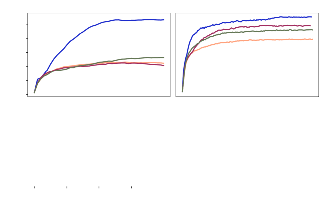
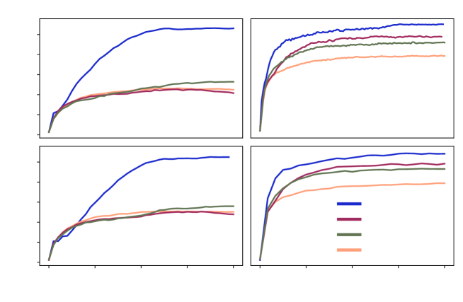
Table 2 compare the performance of our model to all the baselines in various settings with 100 clients. The results show that our algorithm is effective in all settings. The 1000-device experiments confirm our arguments about the large-scale cross-device setting and practicality of AdaBest in comparison to the baselines. Our algorithm has notable gain both in the speed of convergence and the generalization performance. This gain is only overtaken for some benchmarks in full client participation settings (CP=100%) where the best $\beta$ is chosen close to one. According to Remark 5, and the fact that in full participation $\frac{|{\mathcal{P}}^{t}|}{|S^{t}|}=1$ and $t_{i}=t^{\prime}_{i}+1$ for all feasible $i$ and $t$, FedDyn and AdaBest become nearly identical in these settings. In Figure 3, we show the impact of scaling the number of clients in both balanced and imbalanced settings for the same dataset and the same number of clients sampled per round (10 clients). During the hyper-parameter tuning we noticed that the sensitivity of FedDyn and AdaBest to their $\mu$ is small specially for the cases with larger number of clients.

Figure 3: Test accuracy on balanced (top) and unbalanced (bottom) settings for training on 1000 (left) and 100 (right) clients. The training dataset is CIFAR100 and $|{\mathcal{P}}|$=10

Table 2: Mean and standard deviation of test accuracy for various settings. The results are based on 5 random data partitioning seeds. Models are trained for 1k, 1.2k, and 2k rounds, for 1%, 10% and 100% client participation settings, respectively. A smaller $\alpha$ indicates higher heterogeneity. ^∗CP stands for rate of client participation ($\frac{|{\mathcal{P}}|}{|S|}$)

		Top-1 Test Accuracy
$\text{CP}^{*}$	Dataset	Setting	FedAvg	FedDyn	SCAFFOLD	AdaBest
1%	EMNIST-L	$\alpha$=0.03	94.28$\pm$0.07	92.42$\pm$0.14	93.99$\pm$0.16	94.49$\pm$0.07
		$\alpha$=0.3	94.47$\pm$0.10	92.64$\pm$0.31	94.34$\pm$0.23	94.72$\pm$0.22
		IID	94.04$\pm$1.37	92.89$\pm$0.14	94.48$\pm$0.11	94.81$\pm$0.08
	CIFAR10	$\alpha$=0.03	78.18$\pm$0.80	77.91$\pm$0.79	75.83$\pm$2.36	78.44$\pm$1.12
		$\alpha$=0.3	82.21$\pm$0.36	82.06$\pm$0.17	82.96$\pm$0.42	83.09$\pm$0.76
		IID	83.84$\pm$0.17	83.36$\pm$0.39	84.18$\pm$0.26	85.05$\pm$0.31
	CIFAR100	$\alpha$=0.03	47.56$\pm$0.59	46.27$\pm$0.65	47.29$\pm$0.95	47.91$\pm$0.83
		$\alpha$=0.3	49.63$\pm$0.47	50.53$\pm$0.36	52.87$\pm$0.61	53.62$\pm$0.23
		IID	49.93$\pm$0.36	50.85$\pm$0.38	53.43$\pm$0.44	55.33$\pm$0.44
10%	EMNIST-L	$\alpha$=0.03	93.58$\pm$0.25	93.57$\pm$0.20	94.29$\pm$0.11	94.62$\pm$0.17
		$\alpha$=0.3	94.04$\pm$0.04	93.54$\pm$0.22	94.54$\pm$0.11	94.64$\pm$0.11
		IID	94.32$\pm$0.10	93.60$\pm$0.35	94.62$\pm$0.16	94.70$\pm$0.24
	CIFAR10	$\alpha$=0.03	74.04$\pm$0.88	76.85$\pm$0.91	77.19$\pm$1.10	79.64$\pm$0.58
		$\alpha$=0.3	79.74$\pm$0.07	81.91$\pm$0.19	82.26$\pm$0.38	84.15$\pm$0.36
		IID	81.35$\pm$0.23	83.56$\pm$0.31	83.50$\pm$0.15	85.78$\pm$0.14
	CIFAR100	$\alpha$=0.03	39.18$\pm$0.56	44.24$\pm$0.66	45.80$\pm$0.36	48.56$\pm$0.45
		$\alpha$=0.3	38.78$\pm$0.35	48.92$\pm$0.37	46.34$\pm$0.43	54.51$\pm$0.35
		IID	37.45$\pm$0.57	49.60$\pm$0.24	44.30$\pm$0.22	55.58$\pm$0.14
100%	EMNIST-L	$\alpha$=0.03	93.36$\pm$0.15	94.18$\pm$0.21	94.38$\pm$0.20	94.06$\pm$0.11
		$\alpha$=0.3	93.99$\pm$0.19	94.23$\pm$0.14	94.53$\pm$0.16	94.40$\pm$0.21
		IID	94.06$\pm$0.33	94.37$\pm$0.15	94.63$\pm$0.10	94.69$\pm$0.14
	CIFAR10	$\alpha$=0.03	72.97$\pm$1.09	78.24$\pm$0.77	77.64$\pm$0.25	78.07$\pm$0.71
		$\alpha$=0.3	79.12$\pm$0.15	83.19$\pm$0.18	82.26$\pm$0.23	83.20$\pm$0.25
		IID	80.72$\pm$0.33	84.39$\pm$0.20	83.55$\pm$0.25	84.75$\pm$0.17
	CIFAR100	$\alpha$=0.03	38.24$\pm$0.63	46.00$\pm$0.42	46.51$\pm$0.50	46.16$\pm$0.79
		$\alpha$=0.3	37.03$\pm$0.35	50.42$\pm$0.29	45.48$\pm$0.38	50.90$\pm$0.42
		IID	35.92$\pm$0.48	50.61$\pm$0.25	43.73$\pm$0.23	51.33$\pm$0.41

5 Conclusions

In this paper, we introduce AdaBest, an adaptive approach for tackling client drift in Federated Learning. Unlike the existing solutions, our approach is robust to low rates of clients re-sampling, which makes it practical for large-scale cross-device Federated Learning. In benchmarks with a large number of clients, our method outperforms the baselines by a wide margin. The results show nearly a two-fold improvement in test accuracy over the second-best candidate in some cases. Our algorithm consumes no more communication bandwidth or storage than the baselines, and it even has a lower compute cost. AdaBest addresses the instability of norm of gradient estimates used in FedDyn by adapting to the most relevant information about the direction of the client drift. Furthermore, we formulated the general estimate of oracle gradients in a much elegant arithmetic that eliminates the need for the explicit, recursive form used in the previous algorithms.

Future work for this study includes deriving theoretical bounds for our proposed algorithm. Furthermore, in the current paper, the parameter $\beta$ is manually tuned to account for the trade-off between the amount of information retained from the previous estimations of oracle’s gradients and the estimation provided by a new round. Developing a method for automatically tuning $\beta$ is an important direction for improving the proposed algorithm.

Acknowledgments: The first author wishes to express gratitude for the financial support provided by MITACS and Research Nova Scotia. In addition, the fifth author acknowledges Natural Sciences and Engineering research Council of Canada, CHIST-ERA grant CHIST-ERA-19-XAI-0 and the Polish NCN Agency NCN(grant No. 2020/02/Y/ST6/00064). We are grateful to Sai Praneeth Karimireddy, the first author of [9], for enlightening us on the proper implementation of SCAFFOLD. William Taylor-Melanson is also acknowledged for reviewing this paper and providing numerous helpful comments.

Appendix

A Proofs

Remark 1

Aggregating client models by averaging is equivalent to applying a gradient step of size 1 from the previous round’s cloud model using average of client pseudo-gradients or mathematically it is $\bar{{\bm{\theta}}}^{t}\leftarrow\frac{1}{|S^{t}|}\sum_{i\in S^{t}}{\bm{\theta}}_{i}^{t}={\bm{\theta}}^{t-1}-\bar{{\bm{g}}}^{t}$.

Proof

$$\begin{split}\bar{{\bm{\theta}}}^{t}\leftarrow\frac{1}{|S^{t}|}\sum_{i\in S^{t}}{\bm{\theta}}_{i}^{t}&={\bm{\theta}}^{t-1}-\frac{1}{|S^{t}|}\sum_{i\in S^{t}}{\bm{\theta}}^{t-1}-{\bm{\theta}}_{i}^{t}\\ &={\bm{\theta}}^{t-1}-\frac{1}{|S^{t}|}\sum_{i\in S^{t}}{\bm{g}}_{i}^{t}\\ &={\bm{\theta}}^{t-1}-\bar{{\bm{g}}}^{t}\ .\end{split}$$

Theorem A.1

In FedDyn, ${\|{\bm{h}}^{t}\|}^{2}\leq{\|{\bm{h}}^{t-1}\|}^{2}$ requires

$$\cos(\angle({\bm{h}}^{t-1},\bar{{\bm{g}}}^{t}))\leq-\frac{|{\mathcal{P}}^{t}|}{2|S^{t}|}\frac{\|\bar{{\bm{g}}}^{t}\|}{\|{{\bm{h}}}^{t-1}\|}$$

Proof

According to Algorithm 1,

$${\bm{h}}^{t}\leftarrow{\bm{h}}^{t-1}+\frac{|{\mathcal{P}}^{t}|}{|S^{t}|}\bar{{\bm{g}}}^{t}.$$

Applying 2-norm squared on both sides gives

$${\|{\bm{h}}^{t}\|}^{2}={\|{\bm{h}}^{t-1}\|}^{2}+\left(\frac{|{\mathcal{P}}^{t}|}{|S^{t}|}\right)^{(2)}{\|\bar{{\bm{g}}}^{t}\|}^{2}+2\frac{|{\mathcal{P}}^{t}|}{|S^{t}|}\langle{\bm{h}}^{t-1},\bar{{\bm{g}}}^{t}\rangle.$$

Considering the proposition, we have

$$\therefore\ {\|{\bm{h}}^{t}\|}^{2}\leq{\|{\bm{h}}^{t-1}\|}^{2}\implies\ 2\langle{\bm{h}}^{t-1},\bar{{\bm{g}}}^{t}\rangle\leq-\frac{|{\mathcal{P}}^{t}|}{|S^{t}|}{\|\bar{{\bm{g}}}^{t}\|}^{2}.$$

with dividing both sides on some positive values, we get

$$\frac{\langle{\bm{h}}^{t-1},\bar{{\bm{g}}}^{t}\rangle}{\|\bar{{\bm{g}}}^{t}\|\|{{\bm{h}}}^{t-1}\|}\leq-\frac{|{\mathcal{P}}^{t}|}{2|S^{t}|}\frac{\|\bar{{\bm{g}}}^{t}\|}{\|{{\bm{h}}}^{t-1}\|},$$

which is equivalent to the

$$\cos(\angle({\bm{h}}^{t-1},\bar{{\bm{g}}}^{t}))\leq-\frac{|{\mathcal{P}}^{t}|}{2|S^{t}|}\frac{\|\bar{{\bm{g}}}^{t}\|}{\|{{\bm{h}}}^{t-1}\|}.$$

Remark 2

$\bar{{\bm{\theta}}}^{t-1}-\bar{{\bm{\theta}}}^{t}$ is equivalent to ${\bm{h}}^{t-1}+\bar{{\bm{g}}}^{t}$ in AdaBest.

We first add and remove ${\bm{\theta}}^{t-1}$ from the first side of the equation,

$$\begin{split}\bar{{\bm{\theta}}}^{t-1}-\bar{{\bm{\theta}}}^{t}&=\bar{{\bm{\theta}}}^{t-1}-\bar{{\bm{\theta}}}^{t}+{\bm{\theta}}^{t-1}-{\bm{\theta}}^{t-1}\\ &=(\bar{{\bm{\theta}}}^{t-1}-{\bm{\theta}}^{t-1})+({\bm{\theta}}^{t-1}-\bar{{\bm{\theta}}}^{t}).\end{split}$$

Then, we replace some terms using Equation 1 and Remark 1 to get

$$\begin{split}\bar{{\bm{\theta}}}^{t-1}-\bar{{\bm{\theta}}}^{t}={\bm{h}}^{t-1}+\bar{{\bm{g}}}^{t}.\end{split}$$

Remark 3

Cloud pseudo-gradients of AdaBest form a power series of ${\bm{h}}^{t}=\sum_{\tau=0}^{t}\beta^{(t-\tau+1)}\bar{{\bm{g}}}^{\tau}$, given that superscript in parenthesis means power.

Proof

We make the induction hypothesis ${\bm{h}}^{t-1}=\sum_{\tau=0}^{t-1}\beta^{(t-\tau)}\bar{{\bm{g}}}^{\tau}$. We need to prove that ${\bm{h}}^{t}=\sum_{\tau=0}^{t}\beta^{(t-\tau+1)}\bar{{\bm{g}}}^{\tau}$. From Algorithm 1 we have

$${\bm{h}}^{t}=\beta(\bar{{\bm{\theta}}}^{t-1}-\bar{{\bm{\theta}}}^{t}).$$

Additionally, using Remark 2 it could be rewritten as

$${\bm{h}}^{t}=\beta({\bm{h}}^{t-1}+\beta\bar{{\bm{g}}}^{t}).$$

Replacing the induction hypothesis changes it to

$$\begin{split}{\bm{h}}^{t}&=\beta(\sum_{\tau=0}^{t-1}\beta^{(t-\tau)}\bar{{\bm{g}}}^{\tau}+\beta\bar{{\bm{g}}}^{t})\\ &=\sum_{\tau=0}^{t-1}\beta^{(t-\tau)}\bar{{\bm{g}}}^{\tau+1}+\beta^{(2)}\bar{{\bm{g}}}^{t}\\ &=\sum_{\tau=0}^{t}\beta^{(t-\tau+1)}\bar{{\bm{g}}}^{\tau}.\end{split}$$

Remark 4

FedAvg is a special case of AdaBest where $\beta=\mu=0$.

Proof

In AdaBest, $\mu=0$ makes ${\bm{h}}_{i}^{t}$ zero for all feasible $i$ and $t$. The resulting local update is identical to that of FedAvg. Similarly, ${\bm{h}}^{t}$ becomes zero at all rounds if $\beta=0$. So AdaBest would also have the same server updates as of FedAvg.

Remark 5

Server update of FedDyn is a special case of AdaBest where $\beta=1$ except that an extra $\frac{|{\mathcal{P}}|}{|S|}$ scalar is applied which also adversely makes FedDyn require prior knowledge about the number of clients.

Proof

According to Algorithm 1, on the server side AdaBest and FedDyn are different in their update of ${\bm{h}}^{t}$. Based on Remark 2, for $\beta=1$ AdaBest update is ${\bm{h}}^{t}\leftarrow{\bm{h}}^{t-1}+\bar{{\bm{g}}}^{t}$. Comparably the same update in FedDyn is ${\bm{h}}^{t}\leftarrow{\bm{h}}^{t-1}+\frac{|{\mathcal{P}}^{t}|}{|S^{t}|}\bar{{\bm{g}}}^{t}$. Involving $\|S^{t}\|$ in the update means assuming that prior knowledge on number of total clients is available from the beginning of the training. On the other hand, $\beta=0$ leads to ${\bm{h}}^{t}=0$ and consequently the update on the cloud model become ${\bm{\theta}}^{t}\leftarrow\bar{{\bm{\theta}}}^{t}$ which is identical to the server update of FedAvg.

Theorem A.2

If $S$ be a fixed set of clients, $\bar{{\bm{\theta}}}$ does not converge to a stationary point unless ${\bm{h}}\rightarrow 0$.

Proof

With a minor abuse in our notation for the case of SCAFFOLD/m (the difference only is applying ${\bm{h}}$ on the clients after ${\bm{\theta}}$ is sent to them), we can generally state that

$$\bar{{\bm{\theta}}}^{t}\leftarrow{\bm{\theta}}^{t-1}-\bar{{\bm{g}}}^{t}=\bar{{\bm{\theta}}}^{t-1}-({\bm{h}}^{t-1}+\bar{{\bm{g}}}^{t}).$$

With $S$ being fixed, upon $t\rightarrow\infty$, and convergence of $\bar{{\bm{\theta}}}$, we expect that ${\bm{g}}^{t}\rightarrow{\bm{0}}$, so the optimization does not step out of the minima. In that case. we also expect $\bar{{\bm{\theta}}}^{t}\approx\bar{{\bm{\theta}}}^{t-1}$. On the other hand, above formula results in $\bar{{\bm{\theta}}}^{t}\approx\bar{{\bm{\theta}}}^{t-1}-{\bm{h}}^{t-1}$ which holds if ${\bm{h}}\rightarrow{\bm{0}}$.

B Algorithm Notation

Following [9] and [2], for the sake of simplicity and readability, we only presented Algorithm 1 for the balanced case (in terms of number of data samples per client). According to [1], SCAFFOLD and FedDyn also need the prior knowledge about the number of clients in order to properly weight their ${\bm{h}}^{t}$ accumulation in the case of unbalance data samples. These weights are used in the form of average samples per client in [1]. We eliminate such dependency in our algorithm by progressively calculating this average throughout the training. We also confirm that applying the same modification on SCAFFOLD and FedDyn does not impede their performance nor their stability (experiments on FedDyn and SCAFFOLD still are done with their original form). For the experiments, we implemented SCAFFOLD as introduced in the original paper [9]; However, for more clarity a modification of it (SCAFFOLD/m) is contrasted to other methods in Algorithm 1 in which only the model parameters are sent back to the server (compare it to Algorithm 1 in [9]). Note that this difference in presentation is irrelevant to our arguments in this paper since the more important factor for scalability in the recursion is $\frac{|S^{t}|-|{\mathcal{P}}^{t}|}{|S^{t}|}$.

C Algorithmic Costs

In this section, we compare compute, storage and bandwidth costs of AdaBest to that of FedAvg, SCAFFOLD/m and FedDyn.

C.1 Compute Cost

Table 3 shows the notation we use for formulating the costs of these algorithms. Algorithm 2 is an exact repetition of Algorithm 1 except that the compute cost of operations of interest are included as comments. These costs are summed in tables Table 4 and Table 5 for the client and server sides, respectively. According to these tables, AdaBest has lower client-side and server-side compute costs than SCAFFOLD/m and FedDyn.

Table 3: Summary of notion used to formulate the algorithm costs

Notation	Meaning
$n\$	Number of parameters of the model $:=|{\bm{\theta}}|$
$g\$	Cost of computing local mini-batch gradients
$s\$	Cost of summing two floating point numbers
$m\$	Cost of multiplying two floating point numbers

Table 4: Comparing AdaBest to FedAvg, SCAFFOLD/m, FedDyn in their compute cost of local (client side) operations. See Algorithm 2 for more detailed comparison

Algorithm	Client side compute cost
FedAvg	$K(g+ns+nm)$
SCAFFOLD/m	$K(g+ns+nm)+2Kns+2n(s+m)$
FedDyn	$K(g+ns+nm)+3Kns+Knm+n(s+m)$
AdaBest	$K(g+ns+nm)+Kns+n(s+m)$

Table 5: Comparing AdaBest to FedAvg, SCAFFOLD/m, FedDyn in their compute cost of global (server side) operations. See Algorithm 2 for more detailed comparison

Algorithm	Server side compute cost
FedAvg	$|{\mathcal{P}}^{t}|ns$
SCAFFOLD/m	$|{\mathcal{P}}^{t}|ns+2ns+2nm$
FedDyn	$|{\mathcal{P}}^{t}|ns+3ns+nm$
AdaBest	$|{\mathcal{P}}^{t}|ns+2ns+nm$

C.2 Storage Cost

All the three algorithms require the same amount of storage, on the clients and the server. Each client is supposed to store a set of local gradient estimates with size $n$ (see Table 3), noted as ${\bm{h}}_{i}^{t}$. Likewise, each algorithm stores the same number of variables on the server so that estimates are forwarded to the next rounds. These variables are introduced with ${\bm{h}}^{t}$ in SCAFFOLD/m and FedDyn but with $\bar{{\bm{\theta}}}^{t-1}$ in AdaBest.

C.3 Communication Cost

AdaBest and FedDyn are not different in the way information is communicated between the server and clients; thus, they do not differ in terms of costs of communication bandwidth. That is sending $n$ parameters from server to each selected client at each round and receiving the same amount in the other direction (from each client to the server). The original SCAFFOLD needs doubling the amount of information communicated in each direction ($2n$). However, SCAFFOLD/m reduces this overhead to 1.5 times (of that of AdaBest) by avoiding to send the extra variables from clients’ to the server (1.5 n).

Algorithm 2 Compute cost of SCAFFOLD/m, FedDyn, AdaBest. Operations that are common among all three algorithms are grayed out. The compute cost of other operations are shown with a comment in front of each line. The variables used to represent the cost of each micro-operation are introduced in Table 3

  Input: $T,{\bm{\theta}}^{0},\mu,\beta$

  for $t=1$ to $T$ do

      Sample clients ${\mathcal{P}}^{t}\subseteq S^{t}$.

      Transmit ${\bm{\theta}}^{t-1}$ to each client in ${\mathcal{P}}^{t}$

     Transmit $h^{t-1}$ to each client in ${\mathcal{P}}^{t}$ (SCAFFOLD/m)

     for each client $i\in{\mathcal{P}}^{t}$ in parallel do

        ${\bm{\theta}}_{i}^{t,0}\leftarrow{\bm{\theta}}^{t-1}$

        for $k=1$ to $K$ do

            Compute mini-batch gradients $L_{i}({\bm{\theta}}_{i}^{t,k-1})$ /* $g$ */

           ${\bm{g}}_{i}^{t,k-1}\leftarrow\nabla L_{i}({\bm{\theta}}_{i}^{t,k-1})-{\bm{h}}_{i}^{t^{\prime}_{i}}+{\bm{h}}^{t}$ (SCAFFOLD/m) /* $2ns$ */

           ${\bm{g}}_{i}^{t,k-1}\leftarrow\nabla L_{i}({\bm{\theta}}_{i}^{t,k-1})-{\bm{h}}_{i}^{t^{\prime}_{i}}-\mu({\bm{\theta}}^{t-1}-{\bm{\theta}}_{i}^{t,k-1})$ (FedDyn) /* $3ns+nm$ */

           ${\bm{g}}_{i}^{t,k-1}\leftarrow\nabla L_{i}({\bm{\theta}}_{i}^{t,k-1})-{\bm{h}}_{i}^{t^{\prime}_{i}}$ (AdaBest) /* $ns$ */

            ${\bm{\theta}}_{i}^{t,k}\leftarrow{\bm{\theta}}_{i}^{t,k-1}-\eta{\bm{g}}_{i}^{t,k-1}$ /* $ns+nm$ */

        end for

         ${\bm{g}}_{i}^{t}\leftarrow{\bm{\theta}}^{t-1}-{\bm{\theta}}_{i}^{t,K}$

        ${\bm{h}}_{i}^{t}\leftarrow{\bm{h}}_{i}^{t^{\prime}}-{\bm{h}}^{t-1}+\frac{1}{K\eta}{\bm{g}}_{i}^{t}$ (SCAFFOLD/m) /* $2ns+2nm$ */

        ${\bm{h}}_{i}^{t}\leftarrow{\bm{h}}_{i}^{t^{\prime}_{i}}+\mu{\bm{g}}_{i}^{t}$ (FedDyn) ${\bm{h}}_{i}^{t}\leftarrow\frac{1}{t-t^{\prime}_{i}}{\bm{h}}_{i}^{t^{\prime}_{i}}+\mu{\bm{g}}_{i}^{t}$ (AdaBest) /* $ns+nm$ */

         $t^{\prime}_{i}\leftarrow t$

         Transmit client model ${\bm{\theta}}_{i}^{t}:={\bm{\theta}}_{i}^{t,K}$

     end for

      $\bar{{\bm{\theta}}^{t}}\leftarrow\frac{1}{|{\mathcal{P}}^{t}|}\sum_{i\in{\mathcal{P}}^{t}}{\bm{\theta}}_{i}^{t}$ /* $|{\mathcal{P}}^{t}|ns$ */

     ${\bm{h}}^{t}\leftarrow\frac{|S^{t}|-|{\mathcal{P}}^{t}|}{|S^{t}|}{\bm{h}}^{t-1}+\frac{|{\mathcal{P}}^{t}|}{K\eta|S^{t}|}({{\bm{\theta}}}^{t-1}-\bar{{\bm{\theta}}}^{t})$ (SCAFFOLD/m) /* $2ns+2nm$ */

     ${\bm{h}}^{t}\leftarrow{\bm{h}}^{t-1}+\frac{|{\mathcal{P}}^{t}|}{|S^{t}|}({{\bm{\theta}}}^{t-1}-\bar{{\bm{\theta}}}^{t})$ (FedDyn) /* $2ns+nm$ */

     ${\bm{h}}^{t}\leftarrow\beta(\bar{{\bm{\theta}}}^{t-1}-\bar{{\bm{\theta}}}^{t})$ (AdaBest) /* $ns+nm$ */

     ${\bm{\theta}}^{t}\leftarrow\bar{{\bm{\theta}}}^{t}$ (SCAFFOLD/m)

     ${\bm{\theta}}^{t}\leftarrow\bar{{\bm{\theta}}}^{t}-{\bm{h}}^{t}$ (FedDyn) ${\bm{\theta}}^{t}\leftarrow\bar{{\bm{\theta}}}^{t}-{\bm{h}}^{t}$ (AdaBest) /* $ns$ */

  end for

More accurate costs requires exact specifications of the system design. For example, the aggregation operation on the server if done in a batch (from a buffer of client delivered parameters) requires more storage but can decrease the compute cost using multi-operand adders on floating-point mantissas such as Wallace or Dadda tree adders. However, these design choices do not appear to make a difference in the ranking of the costs for algorithms compared in this paper.

For cost estimates to be more precise, system design specifications must be considered. For instance, using multi-operand adders on floating-point mantissas, such as Wallace or Dadda tree adders, can reduce the compute cost of the aggregation operation on the server if it is performed in a batch (from a buffer of client-delivered parameters) but requires more storage. However, it does not appear that these design decisions affect the ranking of the costs for the algorithms compared in this paper.

D Experiments Details

D.1 Evaluation

There are two major differences between our evaluation and those of prior works.

1. We do not consider number of epochs to be a hyper-parameter. Comparing two Federated Learning (FL) algorithms with different number of local epochs, is unfair in terms of the amount of local compute costs. Additionally, it makes it difficult to justify the impact of each algorithm on preserving the privacy of clients’ data. This is because the privacy cost is found to be associated with the level of random noise in the pseudo-gradients. This randomness in turn is impacted by the number of epochs (see page 8 of [6]). For an example of comparing algorithms after tuning the number of epochs, refer to the Appendix 1 of [2] where 20 and 50 local epochs are chosen respectively for FedAvg and FedDyn in order to compare their performance on MNIST dataset.

2. We consider a hold-out set of clients for hyper-parameter tuning. Although, an on the fly hyper-parameter tuning is much more appealing in FL setting, for the purpose of studying and comparing FL algorithms, it is reasonable to consider hyper-parameters are tuned prior to the main training phase. However, using the performance of the test dataset in order to search for hyper-parameters makes the generalization capability of the algorithms that use more hyper-parameters questionable. Therefore, we set aside a separate set of training clients to tune the hyper-parameters for each algorithm individually. This may make our reported results on the baselines not exactly matching that of their original papers (different size of total training samples).

In addition, we use five distinct random seeds for data partitioning to better justify our reported performance. Throughout all the experiments, SGD with a learning rate of $0.1$ is used with a round to round decay of $0.998$. Batch size of $45$ is selected for all datasets and experiments. Whenever the last batch of each epoch is less than this number, it is capped with bootstrapping from all local training examples (which can further enhances the privacy especially for imbalance settings). We follow [2] in data augmentation and transformation. Local optimization on CIFAR10 and CIFAR100 involves random horizontal flip and cropping on the training samples both with probability of $0.5$. No data augmentation is applied for experiments on EMNIST-L.

D.2 Implementation

We used PyTorch to implement our FL simulator. For data partitioning and implementation of the baseline algorithms, our simulator is inspired from [1] which is publicly shared by the authors of [2]. To further validate the correctness of SCAFFOLD implementation, we consulted the first author of [9]. Additionally, we cross-checked most of the results our simulator yielded to the ones made by [1].

Figure 4: Highlighting the instability of FedDyn and its association with the norm of cloud parameters. The training is performed on a comparably easy FL task but for a large number of communication rounds. Top and bottom subplots show test accuracy (in percentage) and norm of cloud parameters respectively. The horizontal axis which shows number of communication rounds is shared among subplot

Figure 5: Top-1 train and test accuracy score of AdaBest and the baselines. The solid and dash-dotted lines represent train and test, respectively

D.3 Stability and $\|{\bm{\theta}}^{t}\|$

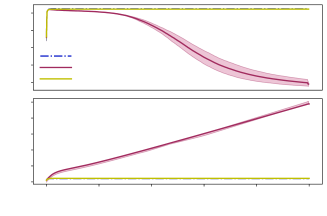
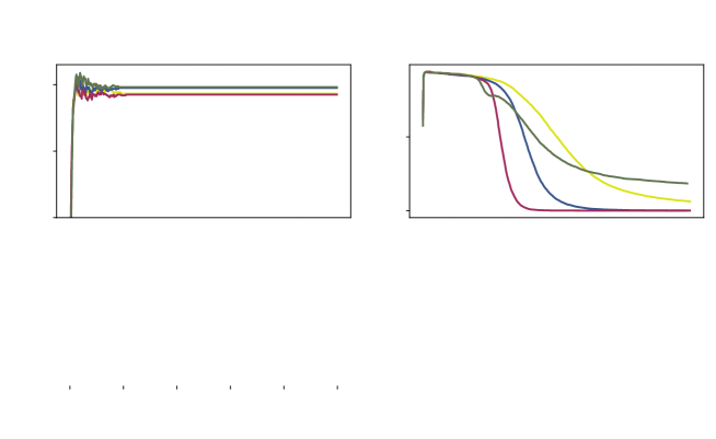
In Figure 1, we showed an experimental case of low client participation to demonstrate how $\|{\bm{\theta}}^{t}\|$ is associated with instability of FedDyn. In this experiment, the training split of CIFAR100 is partitioned over $1100$ clients from which $1000$ is used for training. The partitioning is balanced in terms of number of examples per client and the labels are skewed according to our $\alpha=0.3$ heterogeneity setup (see Section 4.4 for detailed explanation). In each round, $5$ clients are drawn uniformly at random. This low client participation rate is more likely to occur in a large-scale (in terms of number of clients) cross-device FL compared to the setting used for reporting the performances in Table 2 and most of those of our prior works. In Figure 4 we repeat the same experiment; except that a much simpler FL task is defined. In this experiment the training split of EMNIST-L dataset is partitioned into 110 clients, 100 of which are used for training. Partitions are IID (labels are not skewed). Even though this task is much simpler than the previous one, still FedDyn fails to converge when the training continues for a large number of rounds.

D.4 Overfitting Analysis

It is important not to confuse FedDyn’s source of instability with overfitting. To confirm this, we can compare the average train and test accuracy of the same rounds while the model is being trained. Figure 5 compares SCAFFOLD, FedDyn, and AdaBest in this manner. The configuration used in this experiment is identical to the configuration of the experiment in Figure 1, with the exception that it corresponds to a single data partitioning random seed for clarity. The train accuracy is calculated by averaging the train accuracy of participating clients. The results suggest that train accuracy of the baselines is severely declined as the training continues while AdaBest is much more stable in this regard.

D.5 $\mu$-sensitivity

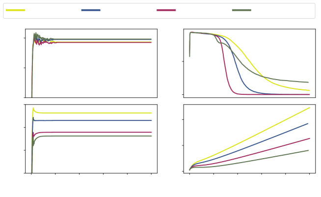
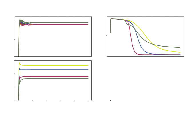
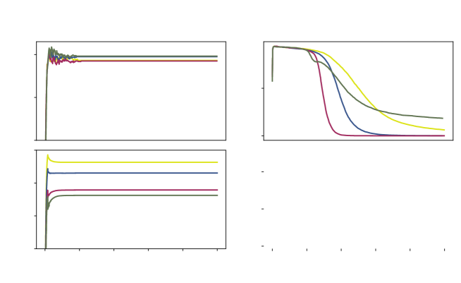
During the hyper-parameter tuning phase, we only tune $\beta$ of AdaBest and set its $\mu$ constantly to $0.02$. This is done throughout all the experiments except the experiment presented in this section which especially investigates the sensitivity of AdaBest to varying $\mu$. Therefore, in practice we have not treated $\mu$ as a hyper-parameter but rather chose the value that works best for FedDyn. For this experiment, we use the same setup as the one presented in Section D.3 on EMNIST-L dataset. The only difference is that we vary $\mu$ in the range of $\{0.02\times 2^{(k)}\}_{k=1}^{k=3}$. Figure 6 depicts the outcome of this experiment along with the result of the same analysis on FedDyn so it would be easy to compare the sensitivity of each of these algorithms to their local factor $\mu$. As suggested by the top left subplot in this Figure, AdaBest can even achieve higher numbers in terms of the test accuracy than what is reported in Table 2. The scales on the vertical axis of the subplots related to AdaBest (on the left column) are zoomed-in to better show the stability of our algorithm throughout the training. On the other hand, the performance and stability of FedDyn shows to be heavily relied on the choice of $\mu$ when the training continues for a large number of rounds.

Figure 6: $\mu$ sensitivity for AdaBest (on the left) and FedDyn (on the right). The horizontal axis which shows the number of communication rounds is shared for each column of subplots. Top and bottom row show the test accuracy (in percentage) and norm of cloud parameters respectively. Note that the vertical axis is not shared as for clarity. This means that the scale of difference between converging point of $\|{\bm{\theta}}^{t}\|$ in AdaBest is largely different from the divergence scale of the same quantity for FedDyn

D.6 $\beta$-sensitivity

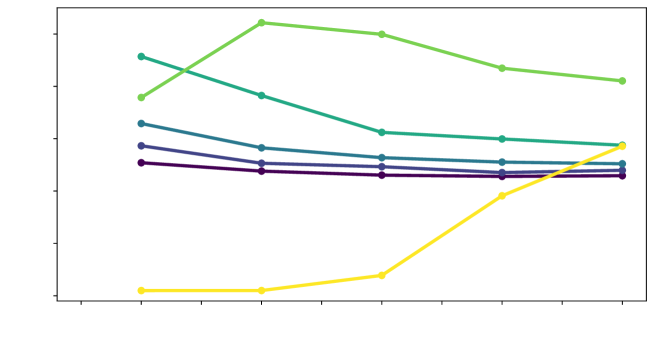
To investigate how the choice of $\beta$ impacts the generalization performance, we conduct an experiment with varying $\beta$ and the rate of client participation. The relation comes from the fact that in lower rates of client participation, the variance of the pseudo-gradients is higher and so a lower $\beta$ is required both in order to avoid explosion of $\|{\bm{\theta}}^{t}\|$ and also to propagate estimation error from the previous rounds as explained in 3.5. For this experiment we use the same setup as the one used in Figure 1 (see Section D.3 for details). Figure 7 implies that when the rate of client participation is $0.005$ ($5$ clients participating in each round out of $1000$ training clients) the optimal $\beta$ is between $0.8$ and $0.95$. With a larger rate of client participation, the optimal value moves away from $0.8$ towards between $0.95$ and $1.0$;

This observation is aligned with our hypothesis on the impact of variance of pseudo-gradients on the estimation error and norm of the cloud parameters. Another interesting point is that for a wide range of $\beta$ values, the performance remains almost stable regardless of the rate of client participation. Additionally, $\beta$ values closer to 1 seem to be suitable for higher rates of client participation, which is suggested by the curve corresponding to $\beta=1.0$ rising as the rate of client participation increases. This case ($\beta=1.0$) is the most similar to formulation of our baselines where the estimations of oracle gradients are not scaled properly from one round to another.

Figure 7: The sensitivity of the test accuracy (in percentage) for different rates of client participation and values of $\beta$. The training is done on a partitioning of CIFAR100 with $1000$ training clients. The numbers on the horizontal axis show the fractions of the total clients sampled at each round

References

- [1] Acar, D.A.E.: Feddyn. https://github.com/alpemreacar/FedDyn (2021), [Accessed 12-Mar-2022]
- [2] Acar, D.A.E., Zhao, Y., Matas, R., Mattina, M., Whatmough, P., Saligrama, V.: Federated learning based on dynamic regularization. In: International Conference on Learning Representations (2020)
- [3] Ajalloeian, A., Stich, S.U.: On the convergence of sgd with biased gradients. arXiv preprint arXiv:2008.00051 (2020)
- [4] Babanezhad Harikandeh, R., Ahmed, M.O., Virani, A., Schmidt, M., Konečnỳ, J., Sallinen, S.: Stopwasting my gradients: Practical svrg. Advances in Neural Information Processing Systems 28 (2015)
- [5] Bi, J., Gunn, S.R.: A variance controlled stochastic method with biased estimation for faster non-convex optimization. In: Joint European Conference on Machine Learning and Knowledge Discovery in Databases. pp. 135–150. Springer (2021)
- [6] Fowl, L.H., Geiping, J., Czaja, W., Goldblum, M., Goldstein, T.: Robbing the fed: Directly obtaining private data in federated learning with modified models. In: International Conference on Learning Representations (2021)
- [7] Hsu, T.M.H., Qi, H., Brown, M.: Measuring the effects of non-identical data distribution for federated visual classification. arXiv preprint arXiv:1909.06335 (2019)
- [8] Johnson, R., Zhang, T.: Accelerating stochastic gradient descent using predictive variance reduction. Advances in neural information processing systems 26, 315–323 (2013)
- [9] Karimireddy, S.P., Kale, S., Mohri, M., Reddi, S., Stich, S., Suresh, A.T.: Scaffold: Stochastic controlled averaging for federated learning. In: International Conference on Machine Learning. pp. 5132–5143. PMLR (2020)
- [10] Konečnỳ, J., Liu, J., Richtárik, P., Takáč, M.: Mini-batch semi-stochastic gradient descent in the proximal setting. IEEE Journal of Selected Topics in Signal Processing 10(2), 242–255 (2015)
- [11] Konečnỳ, J., McMahan, H.B., Ramage, D., Richtárik, P.: Federated optimization: Distributed machine learning for on-device intelligence. arXiv preprint arXiv:1610.02527 (2016)
- [12] Krizhevsky, A., Hinton, G., et al.: Learning multiple layers of features from tiny images. Tech. rep., University of Toronto (2009)
- [13] LeCun, Y., Bottou, L., Bengio, Y., Haffner, P.: Gradient-based learning applied to document recognition. Proceedings of the IEEE 86(11), 2278–2324 (1998)
- [14] Li, D., Wang, J.: Fedmd: Heterogenous federated learning via model distillation. arXiv preprint arXiv:1910.03581 (2019)
- [15] Li, T., Sahu, A.K., Zaheer, M., Sanjabi, M., Talwalkar, A., Smith, V.: Federated optimization in heterogeneous networks. Proceedings of Machine Learning and Systems 2, 429–450 (2020)
- [16] Li, T., Sahu, A.K., Zaheer, M., Sanjabi, M., Talwalkar, A., Smithy, V.: Feddane: A federated newton-type method. In: 2019 53rd Asilomar Conference on Signals, Systems, and Computers. pp. 1227–1231. IEEE (2019)
- [17] Liang, X., Shen, S., Liu, J., Pan, Z., Chen, E., Cheng, Y.: Variance reduced local sgd with lower communication complexity. arXiv preprint arXiv:1912.12844 (2019)
- [18] Lin, T., Kong, L., Stich, S.U., Jaggi, M.: Ensemble distillation for robust model fusion in federated learning. Advances in Neural Information Processing Systems 33, 2351–2363 (2020)
- [19] McMahan, B., Moore, E., Ramage, D., Hampson, S., y Arcas, B.A.: Communication-efficient learning of deep networks from decentralized data. In: Artificial intelligence and statistics. pp. 1273–1282. PMLR (2017)
- [20] Murata, T., Suzuki, T.: Bias-variance reduced local sgd for less heterogeneous federated learning. In: International Conference on Machine Learning. pp. 7872–7881. PMLR (2021)
- [21] Nguyen, L.M., Liu, J., Scheinberg, K., Takáč, M.: Sarah: A novel method for machine learning problems using stochastic recursive gradient. In: International Conference on Machine Learning. pp. 2613–2621. PMLR (2017)
- [22] Pathak, R., Wainwright, M.J.: Fedsplit: An algorithmic framework for fast federated optimization. Advances in Neural Information Processing Systems 33, 7057–7066 (2020)
- [23] Reddi, S.J., Konečnỳ, J., Richtárik, P., Póczós, B., Smola, A.: Aide: Fast and communication efficient distributed optimization. arXiv preprint arXiv:1608.06879 (2016)
- [24] Roux, N., Schmidt, M., Bach, F.: A stochastic gradient method with an exponential convergence _rate for finite training sets. Advances in neural information processing systems 25 (2012)
- [25] Shalev-Shwartz, S., Zhang, T.: Stochastic dual coordinate ascent methods for regularized loss minimization. Journal of Machine Learning Research 14(2) (2013)
- [26] Shamir, O., Srebro, N., Zhang, T.: Communication-efficient distributed optimization using an approximate newton-type method. In: International conference on machine learning. pp. 1000–1008. PMLR (2014)
- [27] Stich, S.U.: Local sgd converges fast and communicates little. In: International Conference on Learning Representations (2018)
- [28] Wang, J., Liu, Q., Liang, H., Joshi, G., Poor, H.V.: Tackling the objective inconsistency problem in heterogeneous federated optimization. Advances in neural information processing systems 33, 7611–7623 (2020)
- [29] Wang, J., Tantia, V., Ballas, N., Rabbat, M.: Slowmo: Improving communication-efficient distributed sgd with slow momentum. arXiv preprint arXiv:1910.00643 (2019)
- [30] Xiao, L., Zhang, T.: A proximal stochastic gradient method with progressive variance reduction. SIAM Journal on Optimization 24(4), 2057–2075 (2014)
- [31] Yu, H., Jin, R., Yang, S.: On the linear speedup analysis of communication efficient momentum sgd for distributed non-convex optimization. In: International Conference on Machine Learning. pp. 7184–7193. PMLR (2019)
- [32] Zhang, X., Hong, M., Dhople, S., Yin, W., Liu, Y.: Fedpd: A federated learning framework with optimal rates and adaptivity to non-iid data. arXiv preprint arXiv:2005.11418 (2020)
- [33] Zhao, Y., Li, M., Lai, L., Suda, N., Civin, D., Chandra, V.: Federated learning with non-iid data. arXiv preprint arXiv:1806.00582 (2018)
- [34] Zhu, L., Han, S.: Deep leakage from gradients. In: Federated learning, pp. 17–31. Springer (2020)
- [35] Zhu, Z., Hong, J., Zhou, J.: Data-free knowledge distillation for heterogeneous federated learning. In: International Conference on Machine Learning. pp. 12878–12889. PMLR (2021)