Termination Shocks and the Extended X-ray Emission in MRK 78

Abstract

Sub-arcsecond imaging of the X-ray emission in the type 2 AGN Mrk 78 with Chandra shows complex structure with spectral variations on scales from $\sim$200 pc to $\sim$ 2 kpc. Overall the X-ray emission is aligned E-W with the radio (3.6 cm) and narrow emission line region as mapped in [OIII], with a marked E-W asymmetry. The Eastern X-ray emission is mostly in a compact knot coincident with the location where the radio source is deflected, while the Western X-ray emission forms a loop or shell $\sim$2 kpc from the nucleus with radius $\sim$0.7 kpc. There is suggestive evidence of shocks in both the Eastern knot and the Western arc. Both these positions coincide with large changes in the velocities of the [OIII] outflow. We discuss possible reasons why the X-ray shocks on the Western side occur $\sim 1$ kpc farther out than on the Eastern side. We estimate that the thermal energy injected by the shocks into the interstellar medium corresponds to $0.05-0.6$% of the AGN bolometric luminosity.

1 Introduction

Energy input from active galactic nuclei (AGNs) is often invoked as a mechanism to regulate star formation in their host galaxies. The discovery of X-ray cavities coincident with radio lobes in cool core galaxy clusters make a strong case for feedback limiting the growth of the most massive galaxies (Dutson et al. 2014; Hlavacek-Larrondo et al. 2015). However, direct evidence of feedback is sparse among the $\sim 90$% of AGN that are radio-quiet (Ivezić et al., 2002). The growth of the central black holes found in almost all non-dwarf galaxies releases enough energy to disrupt star formation if at least $\sim$5% of the AGN power output can be coupled to the galaxy interstellar medium (ISM) (Di Matteo et al. 2005; Hopkins et al. 2006).

Searches for the physical mechanisms which can heat the ISM at this level are ongoing. Powerful molecular outflows capable of suppressing star formation activity have been detected in Mrk 231 (Feruglio et al., 2010) and NGC 1266 (Alatalo et al., 2015) and a number of other AGNs (Fiore et al., 2017), but the driving mechanism of these outflows remains unclear and may differ in different galaxies. Feruglio et al. (2010) find that the kinetic power of the outflow in Mrk 231 is a few percent of the AGN bolometric luminosity and consistent with originating from a highly supersonic shock produced by radiation pressure on the ISM. Alatalo et al. (2015) suggest that the outflow in NGC 1266 is instead more likely to be driven by momentum coupling to the radio jet, and that star formation is suppressed by the injection of turbulence.

It has been suggested that AGN biconical outflows can impart $\sim 5$% of the AGN power into the ISM through termination shocks (Das et al. 2006; Fischer et al. 2011, hereafter F11; Fischer et al. 2013, hereafter F13; Crenshaw et al. 2015). These biconical outflows, modeled from [OIII] line emission data, are randomly inclined with respect to the host galaxy and have large opening half angles of $\approx 30-60^{\circ}$, with thicknesses of $\approx 5-20^{\circ}$ (F13). Such wide bicones are likely to intersect the host disk, interacting with the ISM. All the outflows were modeled quite well with biconical models that are hollow along the central axes, exhibiting a pattern of linear acceleration to a maximum velocity, $v_{\mathrm{max}}$, and then a comparable or faster deceleration beginning at a turnover radius $r_{t}\approx 0.1-1.1$ kpc (F13). More recent models of these outflows have accounted for the rotational kinematics of the host galaxy disk, measuring mean maximum outflow radii of $0.6$ kpc as well as finding that the AGN can disturb the rotational kinematics of the gas out to mean distances of $1.1$ kpc (Fischer et al. 2017; Fischer et al. 2018). In some cases, models have also allowed for outflowing material to be present along the central axis of the bicone when evidence suggests that the outflowing material originates in the galaxy disk (Mrk 573, Revalski et al. 2018a; Mrk 34, Revalski et al. 2018b). The outflows can lose a large fraction of their kinetic energy (up to 75%) over relatively small distances of $\approx 20-200$ pc (F13; Crenshaw et al. 2015; Revalski et al. 2018a; Revalski et al. 2018b; Revalski et al. 2021, hereafter R21).

A plausible explanation for this deceleration is termination shocks due to interaction with the host interstellar medium (ISM), which convert the bulk kinetic energy of the outflow in turbulent motion and radiation. Since no significant increase is observed in the [OIII] line widths beyond $r_{t}$, it is possible that most of the power is radiated away. Given the typical outflow velocities of $v_{\mathrm{max}}\sim 1000$ km s^-1, the expected temperature of the shocked emission is $kT\approx 1.3(v_{\mathrm{shock}}/1000$ km s${}^{-1})^{2}$ keV $\approx 1.3$ keV (Raga et al., 2002), and thus should emit in the soft X-ray band.

Studies of the X-ray emission in NGC 4151 (Wang et al., 2011a), Mrk 573 (Paggi et al., 2012), NGC 1068 Wang et al. (2012), and NGC 3393 (Maksym et al., 2019) using Chandra imaging find evidence of shocked X-ray emission near $r_{t}$ with a wide range of power input from shocks from about $0.05$% of the AGN luminosity in Mrk 573 to $\sim$0.5% in NGC 4151. This level of AGN feedback from shocks may be sufficient to suppress star formation in the two-stage feedback model proposed by Hopkins & Elvis (2010), but is significantly lower than the fraction of accretion power required by most AGN feedback models.

In this paper, we present a study of AGN feedback in Mrk 78 (catalog ) using Chandra imaging. Of the 17 biconical outflows modeled by F13, only three have high $v_{\mathrm{max}}>1000$ km s^-1, corresponding to high $kT$ temperature shocks easily detectable by Chandra, and $r_{t}>0.5^{\prime\prime}$, which can be easily resolved by Chandra. One of these, NGC 1068, was previously observed by Chandra and studied by Wang et al. (2012). The other sources are Mrk 78 (presented here) and Mrk 34 (to be presented in Maksym et al., in prep), for which the modeling by F11 and F13 indicate outflows in the plane of the host disk, so that ISM interactions are highly likely. Both AGN were targeted by a Chandra program in 2017 (on January 1 and 7 for Mrk 78) in order to search for evidence of termination shocks at $r_{t}$ and study their impact on the ISM.

Mrk 78 is classified as an SB Seyfert 2 galaxy in the NASA/IPAC Extragalactic Database (NED). It has a redshift of $z=0.03715$ (Michel & Huchra, 1988), residing at a distance of $\approx 160$ Mpc (for $H_{0}=70$ km s^-1 Mpc^-1). There is evidence that Mrk 78 is heavily obscured based on its X-ray and mid-infrared (IR) properties. Its WISE colors ($W1-W2>0.8$) indicate its mid-IR emission is dominated by AGN-heated dust (Stern et al., 2012), and its 12-micron luminosity ($\nu L_{\nu}$) is $L_{12}\approx 9\times 10^{43}$ erg s^-1. It has been been shown to be nearly Compton-thick based on fitting the broadband X-ray spectrum using XMM and NuSTAR data (Zhao et al., 2020). Its intrinsic $2-10$ keV luminosity is estimated to be $0.8-1.2\times 10^{43}$ erg s^-1 (Zhao et al., 2020), making it consistent with the mid-IR to X-ray correlation from Gandhi et al. (2009).

At a distance of 160 Mpc, 1^′′ corresponds to a physical size scale of 735 pc. The extended narrow-line region (NLR) in Mrk 78 and its relationship to the central radio source have been extensively studied (Whittle et al. 2002; Whittle & Wilson (2004), hereafter WW04; Whittle et al. 2005, hereafter W05; F11). F11 modeled the [OIII] line velocities measured from Hubble Space Telescope Imaging Spectrograph (STIS) spectra using a biconical outflow model. They find $v_{\mathrm{max}}=1200$ km s^-1 and $r_{t}=700$ parsecs. A more recent analysis by Revalski et al. (2021) found a similar best-fit model for the [OIII] outflow, with a slightly larger turnover radius of $r_{t}=900$ parsecs.

However, the outflow in Mrk 78 may be substantially more complex. The [OIII] emission exhibits some high velocities and large line widths beyond the modeled $r_{t}$ on the Western side which are not well described by the outflow model. Furthermore, there is significant asymmetry in both the [OIII] and radio emission on the East and West sides of the nucleus. Based on the radio and [OIII] morphology as well as the [OIII] kinematics, WW04 posited that on the Eastern side, the radio jet is deflected by the ionized gas it encounters and accelerates it. In contrast, they suggest that on the Western side, near to or coincident with where F11 later found large velocities and line widths, the radio jet is disrupted by a compact cloud and expands into a leaky “bubble”, accelerating and ablating ionized gas knots until it blows out of the region through gaps in the gas.

In this paper, we use Chandra imaging of Mrk 78 to search for evidence of shocks, and through comparison of the X-ray, radio, and [OIII] morphologies, better piece together the physical mechanisms by which the central AGN impacts the gas in the host galaxy. In §2, we describe the Chandra observations and pre-existing multi-wavelength data used in this work, as well as their astrometric registration. The production of X-ray images is detailed in §3, and the analysis of the X-ray morphology is discussed in §4. §5 describes the models and methods using for spectral analysis, and §6 provides the spectral results. In §7, we discuss the contribution of the Chandra observations to our understanding of AGN feedback in Mrk 78, especially with regards to the presence and energetics of shocks.

2 Observations and Data Reduction

2.1 Chandra observations

The Chandra X-ray Observatory performed two observations of Mrk 78 in January 2017 with the Advanced CCD Imaging Spectrometer (ACIS). The combined exposure of the two observations is 99.4 ks, and information about the individual observations is provided in Table 1. The observations were analyzed using CIAO 4.11 and CALDB 4.8.3.

Table 1: Chandra Observations

ObsID	R.A. (J2000)	Decl. (J2000)	Start Time	Exposure
	(deg)	(deg)	(UT)	(ks)
18122	115.664589	65.173994	2017 Jan 7 03:50:14	49.85
19973	115.663627	65.173887	2017 Jan 1 21:13:50	49.59

After running the chandra_repro script to process the observations, we checked for background flares in each observation. No significant flares that exceeded the average background rate by $>20\%$ were found. Before combining together the two observations, we improved their relative astrometry. To perform this astrometic correction, we first used the fluximage script to create $0.5-7$ keV images, exposure maps, and PSF maps of the observations and performed source detection using wavdetect in each image. Then, we used wcs_match to calculate the translational offsets between the two Chandra observations by cross-matching the lists of approximately 20 sources detected with $>5\sigma$ significance, excluding Mrk 78. We applied this astrometric adjustment using wcs_update. Finally, merged event files and a $0.3-3$ keV band image was produced using merge_obs.

2.2 [OIII] and 3.6 cm images

In order to build up a more complete view of AGN feedback processes in Mrk 78, in this study we also make use of [OIII] and 3.6 cm images published in WW04. Here we briefly describe how these images were produced, while full details are provided in WW04.

2.2.1 HST [OIII] image

The [OIII] image in WW04 was produced using observations from the pre-COSTAR Planetary Camera on the Hubble Space Telescope (HST). These observations were performed on August 29, 1992, with a total integration time of 5014 seconds in the F517N filter and 1800 seconds in F588N. The F517N filter covers both [OIII] $\lambda 5007$ Å and 4949 Å, while the F588N filter provides a continuum measurement. The continuum was subtracted from the F517N image and the image was then deconvolved. WW04 found that the continuum and line flux measurements based on their images were in excellent agreement with ground-based measurements from de Bruyn & Sargent (1978).

2.2.2 VLA 3.6 cm image

The 3.6 cm image from WW04 was produced from observations by the Karl G. Jansky Very Large Array (VLA) taken in 1990 with A array with a total integration time of 8 hours. The data was flux calibrated. In this work, we use the map that WW04 produced using natural weighting, yielding a beam of $0.29^{\prime\prime}\times 0.27^{\prime\prime}$ in P.A.$=12^{\circ}$ and a noise level of 9 $\mu$Jy beam^-1.

2.3 Astrometric registration

In order to be able to compare the positions of features in the Chandra, HST, and VLA images, it is important for the astrometry of each image to be as accurate as possible. To improve the absolute astrometry of the Chandra observations, we re-ran the CIAO tool wavdetect on the merged $0.3-3$ keV image and searched for multi-wavelength counterparts to all Chandra sources detected with $>5\sigma$ significance using Vizier. We found unique counterparts within 1^′′ for four of the Chandra sources, which are listed in Table 2. We used these counterparts to update Chandra’s astrometry using wcs_match and wcs_update. The average residual offset between the Chandra and optical/infrared counterparts decreased from $0\farcs 52$ to $0\farcs 16$ after this astrometric correction. This average residual offset provides an estimate of the systematic astrometric uncertainty. The peak of the $2-8$ keV emission is located at R.A. = 7:42:41.70, Dec = +65:10:37.46 (J2000); the statistical uncertainty associated with this position is $\pm 0\farcs 07$.

The VLA position of the 3.6 cm radio core is $0\farcs 10$ N and $0\farcs 08$ E of the peak of the $2-8$ keV emission. The VLA positional errors are $\pm 0\farcs 10$, so this position is consistent with the $2-8$ keV peak. Since both the radio core and hard X-ray peak are expected to emanate from the vicinity of the AGN, we shifted the 3.6 cm image so that the radio core and hard X-ray peak coincide, as shown in Figure 1. However, this adjustment is small enough that it does not significantly impact our results.

For the HST image, we adopt the same astrometry as WW04, who assumed no astrometric offset between the F517N and F588N images and fixed the HST F588N continuum peak to the ground-based blue-green continuum peak (Clements, 1981). The optical continuum peak is located at a distance of $0\farcs 13$ from the 2-8 keV peak, which is consistent within the errors. Since Mrk 78 has a prominent dust lane, seen in the blue F342W FOC image shown in WW04, it is possible for the hard X-ray peak and the optical continuum peak not to coincide due to obscuration. Therefore, we do not adjust the astrometry of the optical images to force these two peaks to coincide.

Table 2: Optical and infrared counterparts used for astrometric registration

Catalog	R.A. (J2000)	Decl. (J2000)	Initial offset from Chandra	Magnitudes
	(deg)	(deg)	(arcsec)	(Vega)
AllWISE	115.6634718	65.1474536	0.70	W1=$16.41\pm 0.06$, W2=$15.7\pm 0.1$, W3=$12.2\pm 0.3$
Gaia	115.753066	65.185329	0.56	G=$20.67\pm 0.01$, BP=$20.73\pm 0.08$, RP=$19.48\pm 0.05$
Gaia	115.819352	65.158297	0.25	G=$19.734\pm 0.006$, BP=$19.85\pm 0.04$, RP=$19.29\pm 0.04$
USNO-B1.0	115.631550	65.215975	0.57	B1=20.46, R1=18.85, B2=19.68, R2=18.56
Notes: References for catalogs: AllWISE (Cutri & et al., 2013), Gaia DR2 (Gaia Collaboration 2018), USNO-B1.0 (Monet+2003)

Figure 1: Chandra $2-8$ keV image binned by 1/8 subpixel and adaptively smoothed. VLA 3.6cm contours are shown in white. The radio core has been aligned with the $2-8$ keV peak shown by the black cross.

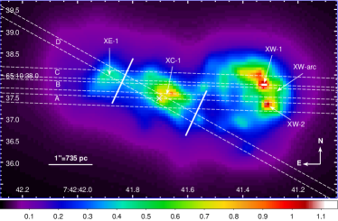
Figure 2: Chandra $0.3-2$ keV image binned by 1/8 subpixel and adaptively smoothed. The location of the $2-8$ keV peak is shown by a white cross. The white solid lines indicate the turnover radius of the [OIII] outflow model from F11, and the white dashed lines show the STIS slit locations and slit names as used by F11. Soft X-ray features are labeled to facilitate discussion in the text.

3 Imaging Analysis

After astrometrically registering the Chandra observations, we produced images in the $0.3-2$ keV and $2-8$ keV bands with 1/8 pixel scale to study the detailed structure of the emission at the center of Mrk 78. We adaptively smoothed the images with the ciaoadapt tool in ds9, using Gaussian smoothing kernels with radii ranging from $0.5-15$ pixels. Comparing the results using different values of the minimum counts under each kernel, we find that a value of 11 counts reveals the highest resolution features that consistently appear in smoothed images. The resulting $0.3-2$ keV and $2-8$ keV smoothed images are shown in Figures 1-4. Figure 2 includes labels for prominent soft X-ray features.

We explore how the morphology of the soft X-ray emission varies with energy. We produced adaptively smoothed images in the $0.3-1$ keV and $1-2$ keV bands, in the same manner as described above but with a lower minimum count per kernel value of 10. These images are included in the three-color X-ray image shown in Figure 3. In order to search for possible evidence of shocked emission, we also made a map of the $0.82-0.92$ keV band, the redshifted energy of the Ne IX line (rest-frame=0.905 keV), which is often observed in shocked emission regions, correlated with radio jets in other AGN (e.g., NGC4151, Wang et al. 2011b, a, c; Mrk 573, Paggi et al. 2012; NGC 3393, Maksym et al. 2019). This smoothed map, shown in Figure 5, is made in the same manner as the other images, except that the minimum counts per kernel value was lowered to 5.

In addition, since the $L$[OIII]/$L_{\mathrm{X}}$ ratio can help distinguish between photionized and shock-ionized emission (Bianchi et al. (2006), (Wang et al., 2012)), we also made a map of the $L$[OIII]/$L_{\mathrm{X}}$ ratio. This map was made by binning both the [OIII] and $0.5-2$ keV images by the same grid of $0\farcs 246$ pixels using the CIAO tool reproject_image_grid. The $0.5-2$ keV counts image was converted into a flux image using a conversion factor of $8.35\times 10^{-17}$ erg s^-1 cm² photon^-1 based on spectral fitting of the total $0.5-2$ keV emission of Mrk 78 (see §5). Then using dmimgcalc, we divided the [OIII] flux image by the $0.5-2$ keV flux image to obtain the $L$[OIII]/$L_{\mathrm{X}}$ ratio map shown in Figure 7.

4 Imaging Results

4.1 X-ray morphology

As can seen in Figure 2, the $0.3-2$ keV emission at the center of Mrk 78 is extended, especially in the E-W direction. There is a bright knot of $0.3-2$ keV emission labeled XC-1 in Figure 2 that is roughly 1^′′ across in the vicinity of the nucleus. As expected given that Mrk 78 hosts an obscured Seyfert 2 AGN, this emission does not originate directly from the innermost part of the AGN (i.e. accretion disk or corona) as evidenced by the fact that it is not centered on the peak of the $2-8$ keV emission and it has a more asymmetric profile than expected for the Chandra PSF. The morphology of the extended emission more than $1^{\prime\prime}$ away from the Mrk 78 nucleus is very different on the Eastern and Western sides. On the Eastern side, the emission is fairly compact, peaking in knot XE-1 located about $1\farcs 3$ (950 pc) from the nucleus. On the Western side, the emission spreads out into a wider feature, extending about $3\farcs 0$ (2200 pc) from the nucleus and exhibiting a curved arc of X-ray emission about $1^{\prime\prime}$ in length on the outer edge, with two particularly bright X-ray knots, labeled XW-1 and XW-2 in Figure 2.

The observed X-ray morphology is most likely associated with interactions between the AGN and the surrounding medium. It is unlikely that the X-ray emission is associated with star formation as the host galaxy of Mrk 78 exhibits optical spectral signatures indicative of being in a post-starburst phase with stellar populations $>10^{8}$ years old (Cid Fernandes et al., 2001). The X-ray morphology of Mrk 78 is also unlikely to be affected by external factors such as ongoing mergers given that no low surface brightness extended features have been detected (Smirnova et al., 2010), and that the nearest neighboring galaxy appearing in R-band images of Mrk 78 has a much higher spectroscopic redshift of $z=0.38$ (Kozlova et al., 2020).

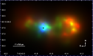
Figure 3: Adaptively smoothed three-color X-ray image showing the $0.3-1$ keV band in red, $1-2$ keV band in green, and $2-8$ keV band in blue. The cross represents the peak of the $2-8$ keV emission. All images are linearly scaled between a minimum value of zero counts and a maximum value of 0.3, 0.6, and 2.0 counts per pixel for the $0.3-1$, $1-2$, and $2-8$ keV bands.

Figure 4: Both panels display the $0.3-2$ keV smoothed counts image with 1/8 subpixel binning. In panel (a), the white contours show the [OIII] emission, and the cross represents the peak of the $2-8$ keV emission. In panel (b), the white contours show the 3.6 cm emission.

4.2 X-ray morphological variation with energy

The X-ray morphology of the extended emission varies with energy. As shown in Figure 3, the the extended emission located $\lesssim 2^{\prime\prime}$ from the nucleus is harder, having a higher ratio of $1-2$ keV flux to $0.3-1$ keV flux, compared to the outer regions of the extended emission. The two X-ray knots on the Western edge, XW-1 and XW-2, also exhibit harder X-ray emission, having a higher ratio of $1-2$ keV flux to $0.3-1$ keV flux than the rest of the arc emission.

The emission within $\pm 50$ eV of the rest-frame Ne IX energy (905 eV) shown in Figure 5 exhibits different morphology than the rest of the $0.3-2$ keV emission shown by the contours. We will refer to this emission in the observed $822-922$ eV band as 900 eV emission. Within $1^{\prime\prime}$ of the nucleus, the 900 eV emission exhibits three faint knots which are offset from the central $0.3-2$ keV peak. On the Eastern side, there is a knot of 900 eV emission (XE900-1) roughly coincident with XE-1, which is close to the [OIII] velocity turnover radius from the F11 and R21 outflow models; faint 900 eV emission appears to extend farther to the NE than the bulk of the $0.3-2$ keV emission. On the Western side, the 900 eV emission displays a similar arc as the $0.3-2$ keV emission, but the brightest 900 eV knot XW900-1 is not coincident with either of the two knots (XW-1 and XW-2) within the arc. Thus, some regions of extended emission may exhibit enhanced Ne IX emission, which is indicative of shocks.

Figure 5: Both panels show smoothed counts images of 900 eV emission within $\pm 50$ eV of the NeIX line energy in green/blue and the remainder of the $0.3-2$ keV emission in red. In panel (a), the white contours show the 3 cm contours. In panel (b), the cross represents the peak of the $2-8$ keV emission, the white lines indicate the turnover radius of the [OIII] outflow model from F11, the cyan regions show the 900 eV spectral extraction regions near the nucleus and the red regions indicate the 900 eV spectral extraction regions farther out from the nucleus. The colorbar values shown correspond to the red color image; the scale for the green/blue image is approximately a factor of 7.5 lower than for the red image.

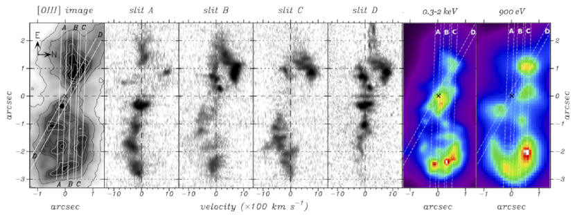
Figure 6: From left to right, images of the [OIII] emission, the [OIII] velocity field in the four STIS slits, the $0.3-2$ emission, and the 900 eV emission. The positions of the STIS slits are overlayed on the [OIII] and X-ray images. The color scales of the X-ray images are chosen so that key features are easily visible; the colorbar values of the 900 eV emission are a factor of 10 lower than those of the $0.3-2$ keV emission.

4.3 Comparison of X-ray, [OIII], and radio morphology

As shown in Figure 4, the E-W asymmetry of the soft X-ray emission resembles the asymmetry seen in the [OIII] and 3.6 cm maps. On the Eastern side, the X-ray, [OIII], and radio knots are in close proximity to one another; the peak of the X-ray emission (XE-1) lies farther from the nucleus than the peak of the [OIII] emission. However, the X-ray emission does not extend as far to the NE as the [OIII] emission, but is truncated at roughly the location where the radio emission begins to bend towards the SE.

On the Western side, both the [OIII] and radio maps show a “bubble”-like morphology similar to the soft X-rays. However, in detail their morphology differs. There are several significant knots of [OIII] emission between $1-2^{\prime\prime}$ from the nucleus, where both the soft X-ray and radio emission is relatively low. Both the X-ray and [OIII] emission exhibit a bright, curved arc $2-3^{\prime\prime}$ West of the nucleus, however the two brightest X-ray knots within this region (XW-1 and XW-2) are offset from the [OIII] peaks within this arc. The radio emission is bright on the inside and outside of this curved arc and in between the two brightest X-ray knots within the arc. These two X-ray knots coincide with areas where the radio emission appears “pinched” towards the center of the E-W radio axis. The 900 eV peaks (XW900-1, XW900-2) in the Western arc also roughly coincide with bright [OIII] emission in the Western arc and the location where the Western radio emission is pinched, as can be seen in Figure 5.

The white lines in Figure 2 show the location of the turnover radius from the modeling of the [OIII] outflow by F11 and R21. This is the location at which the outflow model reaches maximum velocity and then begins to decelerate. Near this radius, there is a knot of X-ray emission on the Eastern side of the nucleus, but an overall dearth of X-ray emission on the Western side. This radius appears to coincide with changes in the radio morphology, with the bending of the radio jet on the Eastern side and the beginning of the jet’s expansion into a wider structure on the Western side.

Figure 6 compares the [OIII] velocity field in each of the four HST STIS slits, the $0.3-2$ keV emission, and the 900 eV emission. As can be seen, the large [OIII] velocity decrease seen $1^{\prime\prime}$ East of the nucleus in all the slit velocity fields coincides with the location of the Eastern knot XE-1, visible both in $0.3-2$ keV and 900 eV emission maps. Another large [OIII] velocity drop is visible $2^{\prime\prime}$ West of the nucleus in slit C, which coincides with the brightest 900 eV knot XW900-1. This velocity drop is not accounted for by the F11 or R21 [OIII] biconical outflow models, indicating that this model may be an incomplete description of the [OIII] outflow kinematics and that Mrk 78 may require more complex modeling as has been more recently performed for other AGN (Fischer et al. 2017;Fischer et al. 2018; Revalski et al. 2018a; Revalski et al. 2018b).

4.4 The $L$[OIII]/$L_{\mathrm{X}}$ ratio

As shown in Figure 7, the extended emission of Mrk 78 shows a range of $L$[OIII]/$L_{\mathrm{X}}$ values, with values generally decreasing outwards along the cross-cone direction. Bianchi et al. (2006) modeled the dependence of the $L$[OIII]/$L_{\mathrm{X}}$ ratio for photoionized emission on the ionization parameter, $U=Q_{\mathrm{ion}}/(4\pi r^{2}cn_{e})$, where $Q_{\mathrm{ion}}$ is the number of hydrogen-ionizing photons emitted by the central object per second and $r$ is the distance to the central ionizing source. If $U$ decreases with increasing radius from the source, $L$[OIII]/$L_{\mathrm{X}}$ is expected to increase, whereas if $U$ increases with radius, $L$[OIII]/$L_{\mathrm{X}}$ is expected to decrease. As discussed in §6.2, our spectral analysis reveals that $U$ is either roughly constant or decreases with distance from the AGN. Therefore, the lower values of $L$[OIII]/$L_{\mathrm{X}}$ in the Western arc cannot be explained by trends in the photoionization parameter.

One factor which can result in lower $L$[OIII]/$L_{\mathrm{X}}$ ratios than expected from photoionization is the presence of shocks (Wang et al. 2012; Maksym et al. 2019). As discussed in §7.3, shocks may be responsible for the low $L$[OIII]/$L_{\mathrm{X}}$ in the Western arc. Another factor which can result in lower $L$[OIII]/$L_{\mathrm{X}}$ ratios is obscuration; the low $L$[OIII]/$L_{\mathrm{X}}$ ratios in the cross-cone regions North and South of the nucleus are consistent with the presence of a dust lane visible in optical images which obscures the optical emission more than the soft X-ray emission.

Figure 7: Map of $L$[OIII]/$L_{\mathrm{X}}$ ratio, where $L_{\mathrm{X}}$ is measured in the $0.5-2$ keV band. The white contours display the 3.6 cm emission contours. The black lines denotes the region outside of which both the $0.3-2$ keV and [OIII] emission is low and thus the ratio values are not significant.

5 Spectral Analysis

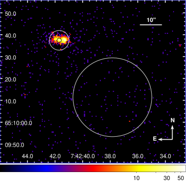
Figure 8: 0.3-2 keV raw counts image. The large $18^{\prime\prime}$-radius circle shows the background extraction region using for all our spectra. A $1^{\prime\prime}$-radius circle shows the source region for the Mrk 78 nucleus, while the annulus with outer $4\farcs 5$-radius shows the source region encompassing all the extended emission.

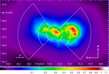
Figure 9: 0.3-2 keV smoothed image with spectral extraction regions shown in white. The cross shows the peak of the $2-8$ keV emission. The spectrum of the Mrk 78 nucleus is extracted from the circular region. We extract spectra separately from the inner and outer regions of extended emission using the pie sector slices shown.

We analyzed the spectrum of the soft X-ray emission to investigate its origin, in particular whether it arises from photoionization by the central AGN or collisional ionization, possibly associated with shocks. Given the spatial variation of the X-ray properties discussed in §3, we analyzed and compared the X-ray spectrum of different emission regions. Figure 8 shows the $18^{\prime\prime}$-radius circular background extraction region we used for all the spectra, which lies on the same ACIS-S chip as Mrk 78 and avoids any sources detected by wavdetect. This figure also displays the $1^{\prime\prime}$-radius circular region used to extract the spectrum of the Mrk 78 nucleus and the $1^{\prime\prime}$ - $4\farcs 5$-radius annular region encompassing the total extended soft X-ray emission. As shown in Figure 9, we further split up this annular region into Eastern and Western pie sectors along the bi-cone axis; these sectors are divided into inner and outer regions that are $1-2^{\prime\prime}$ and $2-4.5^{\prime\prime}$ from the nucleus, respectively. The inner regions have higher $L$[OIII]/$L_{\mathrm{X}}$ ratios and higher fractions of $1-2$ keV flux compared to $0.3-1$ keV flux, appearing green in Figure 3.

In addition, we also independently analyzed the spectra of regions with enhanced 900 eV emission. Based on Figure 5, we identified spectral regions that exhibit elevated 900 eV emission compared to the bulk of the $0.3-2$ keV emission; these are the regions that appear cyan in Figure 5. We selected as many of these regions as possible in order to obtain as many counts as possible for spectral analysis. We analyzed regions within $1^{\prime\prime}$ of the nucleus (shown by cyan shapes) separately from those farther out from the nucleus (shown by red shapes), since we found that the $0.3-2$ keV emission differs significantly in these regions as discussed in §5.

We extract the spectrum of each source region and corresponding ARF and RMF files using specextract. We bin each spectrum so that each energy bin has at least 15 counts, and use chi-squared statistics when fitting the spectra. We find that fitting the spectra binned by a minimum 5 counts per bin using the L-statistic (“lstat” in XSPEC (Arnaud, 1996)), which is appropriate for Poissonian data with Poissonian background, produces consistent results.

In our spectral analysis of the soft X-ray emission, we use the XSPEC apec model to represent the thermal continuum and line emission from collisionally-ionized diffuse gas. We freeze the relative metal abundances for these thermal models to solar values from Anders & Grevesse (1989). To model photoionized gas emission we used an XSPEC grid of models produced using the CLOUDY c08.01 package (Ferland et al., 1998). This model grid is the same as that used by Paggi et al. (2012) and Maksym et al. (2019) in studies of the soft X-ray emission associated with AGN in Mrk 573 and NGC 3393. The ionization source for this CLOUDY grid was assumed to be an AGN continuum with a “big bump” temperature of $10^{6}$ K, an X-ray to UV ratio $\alpha_{OX}=-1.30$, and an X-ray powerlaw component with spectral index $\alpha=-0.8$. The emitting cloud was assumed to have plane-parallel geometry and constant electron density $n_{e}=10^{5}$ cm^-3. Note that the fraction of ionized species and equilibrium populations of excited states for key elements are expected to be similar for electron densities $n_{e}\sim 1-10^{6}$ cm^-3 (Porquet & Dubau 2000; Ferland et al. 2017). The model grid was parametrized in terms of the ionization parameter ($U=Q_{\mathrm{ion}}/(4\pi r^{2}cn_{e})$) over the range log$U$=[-3.0:2.0] in steps of 0.25 and the hydrogen column density ($N_{\mathrm{H}}$) over the range log$N_{\mathrm{H}}$=[19.0:23.5] in steps of 0.1.

For each spectrum, we begin by fitting a single component model subject only to Galactic absorption, which we estimate using the COLDEN tool to be $N_{\mathrm{H,Gal}}=4.1\times 10^{20}$ cm^-2. More components were added, one at a time if: (1) the best fit resulted in a reduced chi-squared value $\chi_{\nu}^{2}>2$, (2) a null hypothesis probability, $p_{\mathrm{null}}<5$%, or (3) there was significant structure in the residuals. This process was continued until a good fit was produced.

6 Spectral Results

6.1 Mrk 78 Nucleus

Figure 10: Spectrum of Mrk 78 nucleus. The model fits shown all include Galactic obscuration, a power-law component and two Gaussian lines. In addition, (a) includes one photoionization component, (b) includes additional obscuration associated with Mrk 78, and one thermal component, and (c) includes two thermal components. The best fit parameters are shown in Table 3.

The spectrum of the nuclear region of Mrk 78 is shown in Figure 10. At energies $>2$ keV, the spectrum is well described by a hard power-law component and two Gaussian lines. The strongest line has a central energy of $6.44\pm 0.05$ keV, the energy of neutral Fe K$\alpha$. The hard power-law and strong iron emission is typical of obscured AGN. If this line is excluded from the model, $\chi_{\nu}^{2}=2.8$ and the model is ruled out with $>6\sigma$ confidence.

Visual inspection of the residuals suggests that there may also be a second Gaussian line at approximately 5.2 keV. When fitting just the $3-8$ keV band, including this additional line reduces $\chi^{2}_{\nu}$ from 1.30 to 1.14 and increases the null hypothesis probability ($p_{\mathrm{null}}$) from 15% to 29%. The central energy of this line is consistent with the 5.17 keV line seen reported in the Compton-thick AGN in NGC 7212 (Jones et al., 2020). It was suggested this line could result from He-like Vanadium formed by cosmic spallation, although it is debated whether Vanadium K$\alpha$ can be strong compared to other spallation lines and it is debated to what extent spallation may occur in AGN (Skibo 1997; Scott 2005; Turner et al. 2010; Gallo et al. 2019). We note that some structure remains in the residuals around $5-6$ keV, suggesting additional emission lines or non-Gaussian line profiles may be present, but additional X-ray observations would be required to test these possibilities.

Our power-law fits of the AGN continuum should not be taken too literally, since Mrk 78 has been shown to be close to Compton-thick based on X-ray broadband spectral fitting using NuSTAR and XMM observations (Zhao et al., 2020). Zhao et al. (2020) find that the Mrk 78 nucleus exhibits a line-of-sight column density of log($N_{\mathrm{H}}$)$\approx 23.8-23.9$ and that its broadband X-ray spectrum is well-fit by the combination of a thermal component (mekal, Mewe et al. 1985), an absorbed intrinsic cutoff power-law spectrum, a reprocessed component including scattering and fluorescent lines, and leaked unabsorbed intrinsic continuum. They find that the thermal component dominates above the AGN/torus components below 1.5 keV. Given that neither XMM nor NuSTAR can resolve the nuclear and extended emission in Mrk 78, we expect that the AGN/torus emission should be even less dominant in Chandra spectra of the extended emission $>1^{\prime\prime}$ from the nucleus. Therefore, our spectral fitting results of $0.3-2$ keV extended emission should not be significantly impacted by our simple treatment of the AGN continuum. While our spectral fitting results for the nuclear region could be improved by including NuSTAR data, the focus of this paper is the extended emission so we leave this to future work.

Table 3: Nuclear Region Spectral Results

One Photoionization + Power-law	Obscuration * (One Thermal + Power-law)	Two Thermal + Power-law
log($U$)=$1.27^{+0.23}_{-0.22}$	$N_{\mathrm{H}}$=$7.6\pm 1.6\times 10^{21}$ cm-2	kT1=$0.84^{+0.24}_{-0.22}$ keV
log($N_{\mathrm{H}}$)=$22.27^{+0.90}_{-1.94}$	kT1=$0.69^{+0.12}_{-0.13}$ keV	log($f_{0.3-2,\mathrm{apec1}}$)=$-14.33^{+0.19}_{-0.33}$
log($f_{0.3-2,\mathrm{CLOUDY}}$)=$-13.75^{+0.09}_{-0.14}$	log($f_{0.3-2,\mathrm{apec}}$)=$-12.93^{+0.16}_{-0.19}$	kT${}_{2}>3.09$ keV
$\Gamma$=$-0.64^{+0.59}_{-0.42}$	$\Gamma$=$-0.63^{+0.44}_{-0.38}$	log($f_{0.3-2,\mathrm{apec2}}$)=$-13.84^{+0.09}_{-0.07}$
NormPL=$9.1^{+11.2}_{-4.4}\times 10^{-7}$	NormPL=$1.01^{+0.80}_{0.44}\times 10^{-6}$	$\Gamma$=$-1.47^{+0.71}_{-0.99}$
$E_{\mathrm{line},1}$=$6.44^{+0.06}_{-0.05}$	$E_{\mathrm{line},1}$=$6.43^{+0.06}_{-0.05}$	NormPL=$1.9^{+4.6}_{-1.6}\times 10^{-7}$
$\sigma_{\mathrm{line},1}$=$0.24^{+0.10}_{-0.07}$	$\sigma_{\mathrm{line},1}$=$0.23^{+0.09}_{-0.07}$	$E_{\mathrm{line},1}$=$6.43^{+0.06}_{-0.05}$
Normline,1=$7.3^{+1.9}_{-1.7}\times 10^{-6}$	Normline,1=$7.2^{+1.8}_{-1.7}\times 10^{-6}$	$\sigma_{\mathrm{line},1}$=$0.21^{+0.09}_{-0.21}$
$E_{\mathrm{line},2}$=$5.18\pm 0.11$	$E_{\mathrm{line},2}$=$5.18\pm 0.11$	Normline,1=$6.9^{+2.0}_{-4.1}\times 10^{-6}$
$\sigma_{\mathrm{line},2}<0.36$	$\sigma_{\mathrm{line},2}<0.34$	$E_{\mathrm{line},2}$=$5.35^{+1.17}_{-0.27}$
Normline,2=$8.3^{+7.9}_{-5.5}\times 10^{-7}$	Normline,2=$7.8^{+7.5}_{-5.2}\times 10^{-7}$	$\sigma_{\mathrm{line},2}<0.34$
		Normline,2=$1.5^{+3.6}_{-1.1}\times 10^{-6}$
$\chi^{2}$/DOF=57/41	$\chi^{2}$/DOF=56/41	$\chi^{2}$/DOF=51/40
$p_{\mathrm{null}}$=0.053	$p_{\mathrm{null}}$=0.061	$p_{\mathrm{null}}$=0.105
Notes: All models include Galactic absorption with column density $N_{\mathrm{H,Gal}}=4.1\times 10^{20}$ cm-2 and two Gaussian lines. The best-fit value for the equivalent width of the Gaussian line at $5.18$ keV was approximately $0.11$ keV in all three fits.

6.2 Extended soft X-ray emission

In studying the spectrum of the extended soft X-ray emission in Mrk 78, we first test whether the spectra within the Eastern and Western pie sectors along the bi-cone axis shown in Figure 9 are consistent with one another. Fitting the $0.3-2$ keV emission of the East and West regions independently with combinations of two thermal or two photoionization models, we find that the best-fit parameters for the regions are consistent within 1$\sigma$ errors, except for the overall normalization. Thus, in the remainder of our analysis, we combine the spectra from the East and West sides of Mrk 78 to maximize the spectral statistics.

While it would be preferable to treat the two sides independently throughout our spectral analysis due to the morphological differences they exhibit, since we only detect about 800 total counts in the $0.3-2$ keV band from the extended emission, we cannot simultaneously split this X-ray emission between East and West and as a function of radius. We note that when we combine the Eastern and Western X-ray emission, both sides contribute a comparable number of counts to the inner extended emission (between $1-2^{\prime\prime}$ from the nucleus), whereas the Western side contributes 80% of the counts to the combined outer extended emission (between $2-4.5^{\prime\prime}$ from the nucleus). The $L$[OIII]/$L_{X}$ ratios of the East and West sides are are comparable, with the inner extended emission on both sides exhibiting higher ratios than the outer extended emission.

Figure 11: Spectrum of the inner extended emission is shown in red, while that of the outer extended emission is shown in black.

Figure 11 compares the spectra of the inner and outer pie regions shown in Figure 9. The two spectra are well-matched in flux between $1-1.2$ keV but show significant differences. The inner region, shown in red, exhibits lower emission in the $0.3-1$ keV band, different spectral features between $1.2-2$ keV, and higher emission between $4-8$ keV. The latter is due to the fact that the inner region is closer to the AGN, and thus a larger fraction (about 2%) of the counts from the hard X-ray source extend into this region due to the Chandra PSF.

Figure 12: Spectra of inner and outer extended emission regions are shown in red and black, respectively. The model fits shown include two thermal components in (a), three thermal components in (b), two photoionization components in (c) and (d), and a mix of one photoionization and one thermal component in (e) and (f). Best fit parameters are provided in Table 4.

Given the visible differences between the inner and outer region spectra, we fit them independently. We present the results based on fitting the $0.3-2$ keV band in Table 4. At these energies, the contribution from the hard X-ray source is minimal. We find consistent results if we fit the $0.3-8$ keV band, fixing the normalizations of the power-law component and the 6.4 and 5.2 keV lines to the expected contributions from the nuclear hard X-ray source based on the Chandra PSF using the CIAO psfFrac tool.

Neither the inner nor outer $0.3-2$ keV spectra can be well-fit using only a single thermal or photoionization model subject only to Galactic obscuration. The inner region spectrum can be well described with either a single thermal or photoionization model subject to additional, presumably local to Mrk 78, obscuration of $N_{\mathrm{H}}\approx 4.5\times 10^{21}$ cm^-2, or any two component combination of photoionization and/or thermal models without additional obscuration.

The outer region spectrum can also be described well by a combination of either two photoionization models or one photoionization plus one thermal model. In the case of the two photoionization models, the ionization parameters of the outer region are slightly lower than for the inner region, and the photoionization component with relatively lower ionization parameter is more dominant than for the inner region. Using the $2-10$ keV intrinsic luminosity from Zhao et al. (2020) and the AGN SED from Elvis et al. (1994), we estimate $Q_{\mathrm{ion}}\approx 2\times 10^{55}$ ionizing photons per second; thus, the lower ionization parameter log$U\approx 1$ corresponds to $n_{e}\sim 1$ cm^-3, while the higher ionization parameter log$U\approx 2$ corresponds to $n_{e}\sim 0.1$ cm^-3. Note that for this X-ray gas to be in pressure balance with the optical line-emitting gas with $n_{e}\sim 10^{2}-10^{3}$ cm^-3 and $T\sim 10^{4}$ K (W05), a temperature of $\sim 10^{7}$ K would be required, which is reasonable for hot X-ray gas.

When adopting the mixture of one photoionization plus one thermal component, the ionization parameter of the outer region is much lower and its temperature slightly higher than for the inner region; while for the inner region, the photoionization and thermal component contribute the same amount of flux, in the outer region, the photoionization component dominates. The low ionization parameter preferred by this model fit would indicate a higher density of $n_{e}\sim 300$ cm^-3. However, note that it is possible to produce an acceptable fit to the outer region with $\chi^{2}=46$ for 33 degrees of freedom (corresponding to $p_{\mathrm{null}}=0.070$) with an ionization parameter (log$U\approx 1.86$) and thermal temperature($kt\approx 0.75$ keV) that are consistent with the values for the inner region; in this case, the thermal component dominates the flux in the outer region. A model with a single photoionized component subject to obscuration is excluded with $>95$% probability for the outer region.

In order to produce acceptable fits to the outer region using only thermal models, either three thermal without additional obscuration, or two thermal models obscured by $N_{\mathrm{H}}\approx 3.5\times 10^{21}$ cm^-2 in excess of the Galactic values are required. For both these sets of models for the outer region, the lowest temperature thermal component is the most dominant and it has a significantly lower temperature than any of the best-fit thermal components for the inner region. Given that more components are required to fit the spectrum with a thermal-only model compared to photoionization-only or mixed models, and that we know that an AGN photoionizing source is present, it seems unlikely that all the emission in the outer region originates in thermal shocks.

Figure 12 displays the model fits for the inner and outer region based on pure combinations of thermal or photoionization models. The observed and intrinsic fluxes and luminosities of the $0.3-2$ keV emission derived using all the aforementioned models are provided in Table 6.

Table 4: Extended Region Spectral Results

Inner: Two Photoionization		Outer: Two Photoionization
log($U_{1}$)=$1.00^{+0.21}_{-0.15}$	log($U_{2}$)=$1.93^{+>0.07}_{-0.15}$	log($U_{1}$)=$0.75^{+0.10}_{-0.18}$	log($U_{2}$)=$1.87^{+>0.13}_{-0.28}$
log($N_{\mathrm{H,1}}$)=$19.87^{+0.64}_{->0.87}$	log($N_{\mathrm{H,2}}$)$<21.56$	log($N_{\mathrm{H,1}}$)=$19.79^{+0.56}_{-0.52}$	log($N_{\mathrm{H,2}}$)=$19-23.5$
log($f_{0.3-2,1}$)=$-13.65^{+0.11}_{-0.14}$	log($f_{0.3-2,2}$)=$-14.06^{+0.16}_{-0.40}$	log($f_{0.3-2,1}$)=$-13.28^{+0.07}_{-0.05}$	log($f_{0.3-2,2}$)=$-13.88^{+0.14}_{-0.17}$
$\chi^{2}$/DOF=17/12	$p_{\mathrm{null}}$=0.141	$\chi^{2}$/DOF=42/32	$p_{\mathrm{null}}$=0.116
Inner: Two Thermal		Outer: Three Thermal
kT1=$0.67^{+0.16}_{-0.21}$ keV	kT2=$1.60^{+0.79}_{-0.27}$ keV	kT1=$0.12^{+0.08}_{-0.23}$ keV	kT2=$0.84\pm 0.09$ keV
log($f_{0.3-2,1}$)=$-13.85^{+0.10}_{-0.13}$	log($f_{0.3-2,2}$)=$-13.93^{+0.10}_{-0.14}$	log($f_{0.3-2,1}$)=$-13.45^{+0.18}_{-0.23}$	log($f_{0.3-2,2}$)=$-13.59^{+0.07}_{-0.09}$
$\chi^{2}$/DOF=12/13	$p_{\mathrm{null}}$=0.515	kT${}_{3}>2.67$ keV	log($f_{0.3-2,3}$)=$-13.91^{+0.11}_{-0.17}$
		$\chi^{2}$/DOF=32/32	$p_{\mathrm{null}}$=0.464
Inner: One Photoionization + One Thermal		Outer: One Photoionization + One Thermal
log($U_{1}$)=$1.94^{+>0.06}_{-0.16}$	kT2=$0.65^{+0.17}_{-0.16}$ keV	log($U_{1}$)=$-1.41^{+0.50}_{-0.52}$	kT2=$0.90^{+0.09}_{-0.08}$ keV
log($N_{\mathrm{H,1}}$)$<21.34$	log($f_{0.3-2,2}$)=$-13.86^{+0.10}_{-0.11}$	log($N_{\mathrm{H,1}}$)=$20.86^{+1.02}_{-1.11}$	log($f_{0.3-2,2}$)=$-13.60^{+0.07}_{-0.08}$
log($f_{0.3-2,1}$)=$-13.89^{+0.08}_{-0.15}$		log($f_{0.3-2,1}$)=$-13.28^{+0.10}_{-0.15}$
$\chi^{2}$/DOF=12/12	$p_{\mathrm{null}}$= 0.419	$\chi^{2}$/DOF=35/33	$p_{\mathrm{null}}$= 0.370
Inner: Obscuration*(One Thermal)		Outer: Obscuration*(Two Thermal)
kT=$0.58^{+0.14}_{-0.31}$ keV	log($f_{0.3-2}$)=$-13.00^{+0.72}_{-0.17}$	kT1=$0.10\pm 0.04$ keV	kT2=$0.82^{+0.10}_{-0.39}$ keV
$N_{\mathrm{H},z}$=$4.5^{+2.7}_{-1.0}\times 10^{21}$ cm-2		log($f_{0.3-2,1}$)=$-11.99^{+0.46}_{-0.48}$	log($f_{0.3-2,2}$)=$-13.09^{+0.23}_{-0.12}$
$\chi^{2}$/DOF=20/14	$p_{\mathrm{null}}$=0.143	$N_{\mathrm{H},z}$=$3.5^{+1.6}_{-1.2}\times 10^{21}$ cm-2
		$\chi^{2}$/DOF=44/33	$p_{\mathrm{null}}$=0.092
Inner: Obscuration*(One Photoionization)
log($U$)=$0.20^{+0.14}_{-0.16}$	log($f_{0.3-2}$)=$-12.48^{+0.22}_{-0.21}$
log($N_{\mathrm{H}}$)=$19.66^{+0.46}_{->0.66}$	$N_{\mathrm{H},z}$=$4.5^{+1.2}_{-1.0}\times 10^{21}$ cm-2
$\chi^{2}$/DOF=18/13	$p_{\mathrm{null}}$=0.147
Notes: All models include Galactic absorption with column density $N_{\mathrm{H,Gal}}=4.1\times 10^{20}$ cm-2.

We also fit the total $0.3-2$ keV extended emission in an annular region between $1-4.5^{\prime\prime}$ from the nucleus. A combination of at least three thermal or photoionization models are required to fit this spectrum, even if obscuration in excess of Galactic obscuration is included. The only three-component combination that is excluded with $>95$% confidence consists of three photoionization models, which has $p_{\mathrm{null}}=1.5$%. All other possible three-component combinations have a null hypothesis probability $>38$%. However, it is unlikely that all the soft X-ray emission results from collisional thermal processes, since some photoionization due to the central AGN is expected. Thus, it seems most likely that the soft X-ray emission results from a mixture of photoionization and collisional ionization, the latter of which may arise in shocks.

Overall, our spectral analysis reveals that the extended soft X-ray emission in Mrk 78 arises from a complex medium, exhibiting a range of densities and temperatures, as seen in a number of AGN extended X-ray regions (e.g. Travascio et al. 2021; Jones et al. 2020; Fischer et al. 2019; Maksym et al. 2019; Paggi et al. 2012). The photoionization models indicate that the ionization parameter of the photoionized emission is either roughly constant or decreases with distance from the AGN. Since $U\propto n_{e}^{-1}r^{-2}$, this trend implies that the electron density drops off as $r^{-2}$ or less steeply. The optical line emitting gas, which is found to be primarily photoionized, similarly exhibits a decreasing ionization parameter with increasing radius (W05). The thermal models indicate that the low temperature components become more dominant as the radius increases, and the temperature of the collisionally-ionized emission either decreases or remains constant with distance from the AGN.

6.2.1 900 eV emission

In Figure 13, we compare the spectra extracted from the regions with 900 eV emission shown in Figure 5 to the remainder of the extended emission located $>1^{\prime\prime}$ from the nucleus. These spectra are binned with a minimum of only 5 counts per bin, in order to maintain fine energy resolution so that differences between the spectra are more obvious. In order to determine the element species that can account for the differences between the spectra of the 900 eV regions and the remainder of the extended emission, we attempt to fit the $0.3-2$ keV spectra with a combination of Gaussian lines at fixed energies corresponding to species typically seen in ionized AGN bicones (Paggi et al. 2012; Maksym et al. 2019; Jones et al. 2020). The complete list of line energies used can be seen in Table 5.

We perform one set of fits fixing all the line widths to $\sigma=50$ eV. We perform a second set of fits leaving the line width as a free parameter but tieing all the line widths to each other since otherwise there are too many free parameters for meaningful fits. Given the low number of counts per bin, we use the L-statistic to perform the fitting, but also report the chi-square statistic in Table 5 to provide a rough measure of the goodness of fit. We calculate the 90% confidence errors on the free parameters using Monte Carlo Markov chains with 10,000 steps. If a particular line is found to have a normalization upper limit that is $<10^{-8}$, we fix that line normalization to zero and perform the fit again.

We first fit the spectra of the outer 900 eV emission regions and the remainder of the extended emission jointly, allowing for a scaling factor that adjusts the overall normalization but keeps the relative normalizations between different Gaussian lines the same between the two spectra. As can be seen in Figure 14, the two spectra exhibit significantly different residuals to this joint best fit between approximately 0.85 and 1.0 keV. Therefore, we performed a second fit, allowing the normalizations of Gaussian lines in the two spectra in this energy range to be independent of each other. This results in an improved fit, with a lower L-statistic and flatter residuals. Table 5 provides results for the outer 900 eV emission regions, shown in red in Figure 5, and the remainder of the extended emission located $>1^{\prime\prime}$ from the nucleus. Regardless of whether the line width is fixed to 50 eV or left free to vary, the spectrum of the outer 900 eV regions are consistent with enhanced emission around 0.905 keV (the line energy of Ne IX) and lower emission around 1.022 keV (the line energy of Ne X).

The spectra of the outer 900 eV emission regions and the remainder of the extended emission have $300\pm 17$ and $664\pm 26$ net counts in the $0.3-2$ keV band, respectively. Although we analyzed the spectra of the Eastern and Western outer 900 eV regions jointly, we note that there are some differences between the morphology of the 900 eV emission as compared to the [OIII] and radio emission on the Eastern and Western sides. As discussed in §4.3, the 900 eV emission associated with the Eastern knot, XE900-1, lies farther away from the nucleus compared the to the peak of the [OIII] and radio emission on the Eastern side. Instead, in the Western arc, the 900 eV peaks (XW900-1 and XW900-2) are spatially coincident with bright [OIII] and radio emission rather than lying on the outskirts of it. More X-ray data would be required to analyze the spectra of the 900 eV emission in these Eastern and Western regions independently.

The spectrum of the inner 900 eV regions near the nucleus shown in cyan in Figure 5 only have $117\pm 11$ combined net counts in the $0.3-2$ keV band. Modeling the inner 900 eV emission spectrum is further complicated by the fact that the power-law component provides a non-negligible contribution to the $0.3-2$ keV band, requiring additional free parameters in the model. Therefore, we were not able to perform detailed line modeling for the inner 900 eV emission regions.

Nonetheless, we can visually compare their combined spectrum (in blue) in Figure 13 with the spectra of the outer 900 eV emission regions (in red) and the remainder of the extended emission (in black). The inner 900 eV emission regions appear to exhibit the same excess at the Ne IX energy as the outer 900 eV emission regions. However, more X-ray data would be required to make a robust determination.

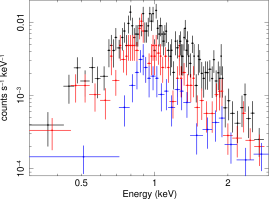
Figure 13: $0.3-3$ keV spectra of the inner and outer sets of 900 eV emission regions (displayed in Figure 5) are shown in blue and red, respectively. The spectrum of the remaining extended emission (excluding the 900 eV emission regions) $>1^{\prime\prime}$ from the nucleus is shown in black.

Figure 14: The spectrum of the outer 900 eV emission regions shown in red in Figure 5 is shown in red, while the spectrum of the remainder of the extended emission at $>1^{\prime\prime}$ from the nucleus is shown in black. The two spectra are fit jointly with a combination of Gaussian lines subject to absorption by a Galactic column density of $4.1\times 10^{20}$ cm^-2. A constant scale factor adjusts the overall normalization of the two spectra. In (a) all lines have a fixed width of $\sigma=50$ eV, and in (b) the line widths are tied together but the value is allowed to vary. Best fit parameters are provided in Table 5.

Table 5: 900 eV Emission Spectral Results

		Joint	900 eV Regions	Remainder	Joint	900 eV Regions	Remainder
		Fixed $\sigma$			Variable $\sigma$
Species	Rest	Normalization	Normalization	Normalization	Normalization	Normalization	Normalization
	Energy (keV)	(1e-6)	(1e-6)	(1e-6)	(1e-6)	(1e-6)	(1e-6)
C V He$\gamma$	0.371	12.15${}^{+12.97}_{-5.72}$	12.65${}^{+2.82}_{-2.17}$		…	…
N VI triplet	0.426	…	…		…	…
C IV Ly$\beta$	0.436	…	…		11.24${}^{+30.35}_{-10.27}$	7.61${}^{+49.24}_{-5.68}$
N VII Ly$\alpha$	0.500	16.03${}^{+18.85}_{-4.28}$	16.11${}^{+2.99}_{-4.83}$		23.60${}^{+9.66}_{-20.98}$	25.76${}^{+9.51}_{-24.16}$
O VII triplet	0.569	7.97${}^{+1.25}_{-2.83}$	8.30${}^{+3.02}_{-0.02}$		…	…
O VIII Ly$\alpha$	0.654	…	…		…	…
Fe XVII	0.720	11.34${}^{+0.88}_{-0.39}$	11.36${}^{+0.05}_{-0.54}$		10.43${}^{+4.26}_{-6.31}$	11.43${}^{+6.31}_{-4.71}$
Fe XVII	0.826	8.58${}^{+0.77}_{-1.75}$	9.28${}^{+0.73}_{-0.72}$		14.70${}^{+4.98}_{-2.74}$	12.87${}^{+4.65}_{4.53}$
Fe XVIII	0.873	…	…		…	…
Ni XIX	0.884	…	…	…	…	…	…
Ne IX	0.905	5.02${}^{+0.19}_{-0.42}$	9.13${}^{+3.29}_{-0.46}$	…	…	5.62${}^{+7.09}_{-5.14}$	…
Fe XIX	0.917	0.87${}^{+1.93}_{-0.85}$	…	$<1.65$	…	…	…
Fe XIX	0.922	…	…	4.19${}^{+0.01}_{-1.39}$	…	…	…
Ne X	1.022	4.85${}^{+0.82}_{-1.85}$	3.78${}^{+1.31}_{-0.06}$	5.21${}^{+0.68}_{-0.54}$	8.29${}^{+1.07}_{-2.07}$	5.93${}^{+3.12}_{-2.88}$	8.23${}^{+2.33}_{-1.01}$
Fe XXIV	1.129	2.48${}^{+0.38}_{-0.17}$	2.56${}^{+0.52}_{-0.97}$		0.37${}^{+1.08}_{-0.33}$	0.92${}^{+0.40}_{-0.79}$
Fe XXIV	1.168	…	…		…	…
Mg XI	1.331	1.82${}^{+0.15}_{-0.33}$	1.85${}^{+0.43}_{-0.50}$		2.14${}^{+0.30}_{-0.67}$	2.06${}^{+0.66}_{-0.29}$
Mg XI	1.352	…	…		…	…
Mg XII	1.478	1.25${}^{+0.37}_{-0.16}$	1.27${}^{+0.05}_{-0.01}$		1.13${}^{+0.49}_{-0.33}$	1.19${}^{+0.40}_{-0.39}$
Mg XII	1.745	0.74${}^{+0.07}_{-0.03}$	0.75${}^{+0.01}_{-0.01}$		0.73${}^{+0.25}_{-0.37}$	0.75${}^{+0.26}_{-0.31}$
Si XIII	1.839	…	…		…	…
Si XIII	1.865	0.42${}^{+0.01}_{-0.02}$	0.43$\pm 0.02$		0.44${}^{+0.31}_{-0.19}$	0.43${}^{+0.34}_{-0.30}$
Si XIV	2.005	0.45${}^{+0.04}_{-0.09}$	0.45${}^{+0.01}_{-0.15}$		0.47${}^{+0.26}_{-0.23}$	0.47${}^{+0.17}_{-0.26}$
Scale factor		0.460${}^{+0.003}_{-0.006}$	0.435${}^{+0.046}_{-0.047}$	1.0	0.459${}^{+0.05}_{-0.042}$	0.437${}^{+0.052}_{-0.070}$	1.0
$\sigma$ (eV)		50	50		87${}^{+9}_{-7}$	82${}^{+12}_{-4}$
L-statistic		111.18	104.57		100.49	96.96
$\chi^{2}$/dof		112.82/102	110.05/100		106.69/104	105.89/102

Table 6: Spectral Region Counts, Fluxes, and Luminosities

Region	Model	Net counts	Net counts	Observed $f_{\mathrm{X}}$	Intrinsic $f_{\mathrm{X}}$	Observed $L_{\mathrm{X}}$	Intrinsic $L_{\mathrm{X}}$
		(0.3-2 keV)	(0.3-8 keV)	($10^{-14}$ erg cm-2 s-1)	($10^{-14}$ erg cm-2 s-1)	($10^{40}$ erg s-1)	($10^{40}$ erg s-1)
Nucleus	1P	$261\pm 16$	$858\pm 29$	$1.77^{+0.15}_{-0.14}$	$1.78^{+0.41}_{-0.49}$	$2.48^{+0.21}_{-0.19}$	$2.49^{+0.58}_{-0.68}$
	O*1T			$1.42^{+0.10}_{-0.09}$	$11.7^{+5.2}_{-4.2}$	$1.98^{+0.14}_{-0.12}$	$16.4^{+7.3}_{-5.8}$
	2T			$1.71^{+0.12}_{-0.68}$	$1.91^{+0.40}_{-0.33}$	$2.39^{+0.17}_{-0.95}$	$2.68^{+0.56}_{-0.46}$
Inner	2P	$294\pm 17$	$383\pm 20$	$2.43^{+0.29}_{-0.12}$	$3.11^{+0.75}_{-0.81}$	$3.40^{+0.41}_{-0.17}$	$4.35^{+1.05}_{-1.13}$
	2T			$2.19^{+0.18}_{-0.11}$	$2.59\pm 0.48$	$3.07^{+0.25}_{-0.15}$	$3.62\pm 0.67$
	1P+1T			$2.25^{+0.16}_{-0.14}$	$2.67^{+0.46}_{-0.47}$	$3.15^{+0.22}_{-0.19}$	$3.74^{+0.65}_{-0.66}$
	O*1T			$1.91^{+0.11}_{-0.13}$	$10.0^{+43.7}_{-3.2}$	$2.68^{+0.15}_{-0.19}$	$14.0^{+61.2}_{-4.5}$
	O*1P			$2.15^{+0.25}_{-0.18}$	$33.1^{+21.8}_{-12.7}$	$3.01^{+0.35}_{-0.25}$	$46.3^{+30.6}_{-17.8}$
Outer	2P	$498\pm 22$	$549\pm 24$	$4.82^{+0.47}_{-0.30}$	$6.57^{+1.03}_{-0.73}$	$6.75^{+0.66}_{-0.42}$	$9.20^{+1.04}_{-0.66}$
	3T			$5.46\pm 0.61$	$7.43^{+1.95}_{-1.62}$	$7.65\pm 0.85$	$10.4^{+2.7}_{-2.3}$
	1P+1T			$5.64^{+0.52}_{-0.43}$	$7.76^{+1.43}_{-1.59}$	$7.89^{+0.73}_{-0.60}$	$10.9^{+2.0}_{-2.2}$
	O*2T			$4.86^{+0.53}_{-0.35}$	$110^{+200}_{68}$	$6.80^{+0.74}_{-0.49}$	$570^{+280}_{-97}$
Notes: Fluxes and luminosities are calculated in the $0.3-2$ keV band. Distance=170 Mpc. Errors on observed properties are 1$\sigma$, on intrinsic are 90%. Model abbreviations: P-photoionization component, O-obscuration in excess of Galactic $N_{\mathrm{H}}$ associated with Mrk 78, T-thermal component.

7 Discussion

7.1 Obscuration within Mrk 78 host galaxy

Based on the models described in §5, the total observed $0.3-2$ keV luminosity arising from thermal or photoionized emission in the nuclear and E-W biconical regions of Mrk 78 ranges from $1.1-1.4\times 10^{41}$ erg s^-1, while the intrinsic $0.3-2$ keV luminosity ranges from $1.5-63\times 10^{41}$ erg s^-1. Including emission in the N-S cross-conical regions increases these estimates by 10%.

The large range in measurements of the intrinsic luminosity arises from uncertainty about whether significant obscuring material within the host galaxy exists. When we allow obscuration associated with the host galaxy to be a free parameter in the spectral models, we find best-fit values of 7.6, 4.5, and 3.5 $\times 10^{21}$ cm^-2 for the nuclear, inner, and outer regions, respectively. F11 measured a reddening of $E(B-V)=0.78$ for the nuclear region of Mrk 78 based on the $H\alpha/H\beta$ ratio from HST STIS spectra. Using the conversion factor from Savage & Mathis (1979), this reddening corresponds to $4.5\times 10^{21}$ cm^-2. Thus, the $N_{\mathrm{H}}$ values measured are reasonable, but since the area covered by the STIS slits and the area of X-ray emission are not the same, we cannot be certain that adopting these $N_{\mathrm{H}}$ values in the X-ray spectral fits is the most appropriate choice. A reddening map of Mrk 78 would allow us to determine appropriate values of $N_{\mathrm{H}}$ in different regions, breaking the degeneracy between obscured and unobscured spectral models, and obtaining more accurate measurements of the intrinsic luminosity.

The column densities observed in the central few kiloparsecs of nearby star-forming galaxies are observed to be $N_{H}\sim 10^{21}-10^{22}$ cm^-2 (e.g. Mineo et al. 2012a; Mineo et al. 2012b; Kahre et al. 2018). The obscuring columns required by the models for Mrk 78 fall in that range.

7.2 Multi-wavelength overview of Mrk 78 emission

Combined with previous studies of the optical gas ionization, morphology, and kinematics (WW04; W05; F11; R21), our X-ray spectral analysis paints a picture in which nuclear radiation is responsible for ionizing the bulk of the [OIII] gas and a significant fraction of the X-ray emitting gas. Both the X-ray and optical gas may be radiatively driven outwards, although it is also possible that the radio flow plays a role in accelerating these phases and sweeping them into an expanding bubble on the Western side as proposed by WW04. In the Western arc, the outflow likely runs into denser gas; compression of the hot gas boosts its emissivity and may partly responsible for the observed bright arc of X-ray emission. However, as discussed in the next section, there is also evidence that some shocked emission exists at bright X-ray knots on both the Eastern and Western sides.

These bright X-ray knots (XE-1, XW-1, XW-2) coincide with regions where both the optical and X-ray gas appear to play a role in channeling the flow of the radio source. At the Eastern knot, XE-1, which is bright both in [OIII] and soft X-rays, the radio flow is deflected and changes direction; a knot of enhanced 900 eV emission (XE900-1) likely associated with Ne IX is located just north of the radio knot. Furthermore, the [OIII] line profile at this knot shows a clear split, which may indicate lateral expansion of the [OIII] gas away from the jet axis (WW04), and the 900 eV emission, which may arise from shocks, is radially exterior to the [OIII] peak. These observations point to very dense gas at the location of the Eastern knot.

In contrast, on the Western side, the outflow is able to expand outwards, likely running into a more extended gas structure farther out from the nucleus at the location of the Western arc. Within the Western arc, bright X-ray (XW-1, XW-2) and [OIII] knots are visible where the radio flow appears pinched; these bright X-ray knots also exhibit enhanced 900 eV emission (XW900-1, XW900-2). Both on the Eastern and Western sides, the bright X-ray knots exhibiting enhanced 900 eV emission indicative of shocks coincide with locations of extreme [OIII] velocity changes of $\sim 1000$ km s^-1.

7.3 Locations of possible shocked emission

A key question which motivated these Chandra observations was whether the deceleration of the [OIII] outflow in Mrk 78 is associated with termination shocks. Our spectral analysis indicates that the soft X-ray emission of Mrk 78 arises from a complex multi-phase medium as evidenced by the fact that a minimum of three model components are required to fit the $0.3-2$ keV extended emission between $1-4.5^{\prime\prime}$ from the nucleus (§6.2). Since the only three-component combination that is strongly disfavored for the extended region is a mixture of three photoionization models, it is likely that at least some shocked emission is present. However, it is important to determine the locations where this shocked emission originates to understand its potential connection to the [OIII] outflow.

While models consisting of only thermal components are disfavored in the outer region, both the inner and outer regions can be well fit by photoionization-only or mixed photoionization plus thermal models. Thus, the spectra of these individual regions do not help to pinpoint where the shocked emission may arise. The only clear difference between the inner and outer regions is that the spectrum of the outer region is overall softer, which can be explained by either lower obscuration and/or an average lower low $kT$ or $U$.

One indicator of shocked emission is enhanced NeIX emission with a rest-frame energy of 905 eV (Paggi et al. 2012;Maksym et al. 2019; Paggi et al. 2022). The strongest enhancements of 900 eV emission are found in the Eastern knot (XE900-1) and the Western arc (XW900-1 and XW900-2). Both of these locations are coincident with a large decrease in [OIII] velocities ($\sim 1000$ km s^-1) as measured by the STIS slits. The Eastern knot also coincides with the location of the [OIII] outflow turnover radius as modeled by F11 and R21. However, on the Western side, at the location of the model turnover radius and the point at which the radio flow begins to widen outwards, there is not a significant excess of 900 eV emission. In fact, this location exhibits only faint X-ray emission, indicating the gas density in this region may be low.

Another indicator of shocked emission are lower $L$[OIII]/$L_{X}$ ratios than expected for photoionized emission. Since our spectral modeling shows that the ionization parameter either decreases or remains constant with radius, if all the X-ray emission results from photoinization, the $L$[OIII]/$L_{X}$ ratio should either remain constant or increase with radius (Bianchi et al., 2006). The Eastern knot coincides with the maximum $L$[OIII]/$L_{X}$ values observed, and therefore, this ratio could be consistent with photoionized emission. However, on the Western side, the $L$[OIII]/$L_{X}$ ratio decreases with distance from the nucleus, and is especially low in the Western arc. This trend is inconsistent with the assumption that all X-ray emission in the Western arc is due to photoionization.

The Eastern knot (XE-1) and the brightest spots of X-ray emission in the Western arc (XW-1 and XW-2), all of which coincide or are adjacent to bright 900 eV emission, also share similar radio morphology. The radio emission appears pinched in the Western arc and pinched and deflected at the Eastern knot, suggesting some significant interaction between the radio-emitting flow and the gas at these locations. Thus, shocks may be present at both of these locations.

7.4 Shock Energetics and Timescales

As discussed in §1, the [OIII] outflow may be decelerated by termination shocks, which we expect to inject thermal energy in the gas and produce thermal X-ray emission. Here we compare the energetics of the [OIII] outflow with those of the possible shocked emission regions.

We first estimate the kinetic power loss associated with the deceleration of the outflow as modeled by F11. The kinetic power is given by $L_{\mathrm{KE}}=0.5\dot{M}v_{\mathrm{max}}^{2}$, where $\dot{M}$ is the mass outflow rate at $r_{t}$. The NLR mass can be estimated as $M_{\mathrm{NLR}}/M_{\odot}=7\times 10^{5}L_{41}(H\beta)/n_{3}$, where $L_{41}(H\beta)$ is the H$\beta$ luminosity in units of $10^{41}$ erg s^-1 and $n_{3}$ is the electron density in units of $10^{3}$ cm^-3 (Peterson, 1997). The H$\beta$ flux of the NLR in a 10^′′-radius aperture is $5.0\times 10^{-14}$ erg cm^-2 s^-1 (Mulchaey et al., 1994). Based on the observed Balmer decrement of $f(H\alpha)/f(H\beta)=6.46$ (Mulchaey et al., 1994), the extinction corrected H$\beta$ luminosity using the Calzetti et al. (2000) dust law is $1.5\times 10^{42}$ erg s^-1; the H$\beta$ luminosity associated with the central $3^{\prime\prime}$-radius region is only a fraction of this total due to the large aperture used for the H$\beta$ measurement. Assuming $n_{3}$=1 based on SII-derived measurements by W05, the NLR mass is $M_{\mathrm{NLR}}=1.1\times 10^{7}M_{\odot}$. The time it takes for the outflow to reach its maximum velocity of $v_{\mathrm{max}}=1200$ km s^-1 at the turnover radius of 700 pc can be found by integrating $\int\frac{dr}{v}$ from the F11 outflow model, which gives an estimate of 4 Myr. Thus, the NLR mass outflow rate is $\lesssim 2.8M_{\odot}$ year^-1, and $L_{\mathrm{KE}}\lesssim 1.3\times 10^{42}$ erg s^-1.

We can compare the estimated kinetic power loss of the [OIII] outflow with the X-ray luminosity and the thermal power associated with the possible shocks in the Western arc and the Eastern knot. For these estimates, we extract spectra from the Western arc and the Eastern knot. We fit these spectra independently, using the models that include thermal components from Table 4 for the outer and inner spectral regions, respectively, fixing all parameters to the best-fit values except the component normalizations. The $0.3-2$ keV luminosity, corrected for absorption, associated with the thermal spectral components of the Western arc is $L_{\mathrm{apec}}\approx 0.04-1.4\times 10^{42}$ erg s^-1. For the Eastern knot, the $0.3-2$ keV luminosity is $L_{\mathrm{apec}}\approx 1-5\times 10^{40}$ erg s^-1.

As an example of our estimates of the thermal power injected into the interstellar medium by shocks, we consider the model with one photoionization and one thermal component with $kT=0.9$ keV from Table 4 applied to the Western arc bright spots. Fitting this model to the Western spectrum, we find an apec normalization of $5\pm 2\times 10^{-6}$. This normalization is proportional to the emission measure: $\frac{10^{-14}}{4\pi[D_{A}(1+z)]^{2}}\int n_{\mathrm{e}}n_{\mathrm{H}}dV$, giving $n_{\mathrm{e}}=0.3$ cm^-3, assuming $n_{\mathrm{e}}\approx n_{\mathrm{H}}$. The thermal pressure is then $p_{\mathrm{th}}\sim 2n_{\mathrm{e}}kT$, and the thermal energy is $E_{\mathrm{th}}=p_{\mathrm{th}}V$, where V is the emitting volume. Assuming that the size of the Western loop along the line-of-sight is comparable to its dimension in the plane of the sky, $1\farcs 2$, the total volume of the bright region of the Western arc is 0.3 arcsec${}^{3}=1.6\times 10^{64}$ cm³. The thermal pressure is then $p_{\mathrm{th}}=1.7\times 10^{-9}$ dyne cm^-2, and the thermal energy is $E_{\mathrm{th}}=1.4\times 10^{55}$ erg. The cooling time of the shocked material is $\tau_{c}=E_{\mathrm{th}}/L_{\mathrm{apec}}=30$ Myr.

The thermal power of the shocks can be derived by estimating the crossing time across the Western arc, which is about $1\farcs 2$ wide in the E-W direction. The thermal velocity of the $0.9$ keV gas is $v_{\mathrm{th}}\sim\sqrt{kT/m_{H}}\sim 290$ km s^-1, which is comparable to the 200 km s^-1 velocity dispersion of the [OIII] gas in this region. Thus, the crossing time is $\approx 3$ Myr, and the thermal power of the shocked region is $L_{\mathrm{th}}=E_{\mathrm{th}}/t_{\mathrm{cross}}\approx 1.6\times 10^{41}$ erg s^-1. Deriving $L_{\mathrm{th}}$ estimates using the other thermal models in Table 4 normalized to the knot spectrum produces values up to a factor of 3 higher than this value ($L_{\mathrm{th}}=5\times 10^{41}$ erg s^-1). Performing the same calculation for the Eastern knot, we estimate the thermal power injected by shocks in this region is $L_{\mathrm{th}}=3-6\times 10^{40}$ erg s^-1.

The total amount of power released either as X-ray emission or thermal motion by the shocks that are likely present in the Western arc and Eastern knot is $0.2-2\times 10^{42}$ erg s^-1. The lower end of this range is based on spectral models with one thermal and one photoionized component, while the higher end assumes that all the soft X-ray emission in these regions has a thermal origin and is significantly obscured. Therefore, the kinetic power lost by the [OIII] outflow may be accounted for by the total amount of power released by the shocks.

7.4.1 On comparing locations of shocked X-ray emission with the [OIII] biconical outflow model

As noted in §7.3, while there is evidence suggestive of shocks in the Eastern knot, at the location of the [OIII] outflow turnover radius of $r_{t}\approx 700-900$ pc from the F11 and R21 bicone models, there is a dearth of X-ray emission 700 pc West of the nucleus. However, significant changes can be observed in the radio outflow about 700 pc West of the nucleus, as the radio flow widens, and we do find evidence for shocks farther out in the Western arc, at roughly 1700 pc from the nucleus.

We consider four plausible explanations for the lack of X-ray emission at the modeled [OIII] turnover radius on the Western side of the outflow:

(1) Given the asymmetric morphology of the outflow on the East and West sides, the [OIII] turnover radius derived from the symmetric biconical models of F11 and R21 may not be appropriate for the Western side. These models in fact do not fit the [OIII] outflow kinematics on the Western side as well as on the Eastern side, although it remains unclear whether this discrepancy may be due to obscuration by dust (F11). Thus, one possibility is that there is no significant bulk deceleration of the outflow $700-900$ pc West of the nucleus, and therefore no X-ray emission arising from shocks near this location. The lack of photoionized X-ray emission in this region may be explained by low gas density and thus correspondingly low X-ray emissivity.

(2) Alternatively, bulk deceleration of the [OIII] outflow may occur as on the Eastern side, but both the [OIII] emission and soft X-ray emission may be obscured. However, more thorough multi-wavelength imaging would be required to evaluate this possibility and determine whether the Western side of the outflow lies behind or in front of the host galaxy disk (F11).

(3) Another possibility is that shocks may occur near the location of the modeled [OIII] turnover radius on the Western side, but they may heat gas to such high temperatures that the gas cannot cool efficiently and thus X-ray emission is only seen farther out in the Western arc once the shock-heated gas has cooled. As in Herbig-Haro object jets, the shocks may heat gas to temperatures $>$2 keV which results in a longer cooling time due to the lack of line emission at these high temperatures. In this case the cooling distance, $d_{cool}$ can be large. Hartigan et al. (1987), Raga et al. (2002), and Heathcote et al. (1998) give $d_{cool}=\frac{100\mathrm{~{}cm}^{-3}}{n_{0}}\frac{v_{shock}}{100\mathrm{~{}km~{}s}^{-1}}$. For typical hot-phase ISM values of $n_{0}=1\mathrm{~{}cm}^{-3}$ and $v_{shock}=1000\mathrm{~{}km~{}s}^{-1}$, $d_{cool}=200\mathrm{~{}pc}$ ($\sim 0\farcs 3$.)

The cooling length formula used for H-H objects is an approximation based on a power law approximation to the radiative cooling coefficient that is appropriate for speeds of a few hundred km s^-1. A better approximation for higher speeds is $d_{cool}~{}=~{}1/4~{}v_{s}~{}t_{cool}$ (John Raymond, 2020, private communication). For a 1200 km s^-1 shock, $T\sim 2\times 10^{7}$ K and $\Lambda=3\times 10^{-23}\mathrm{~{}erg~{}cm}^{3}\mathrm{~{}s}^{-1}$. Then $t_{cool}=5/2(n_{e}+n_{p})kT/(n_{e}n_{p}\Lambda)$ and $n_{e}~{}=~{}n_{p}\sim n_{0}$ gives $\sim$3 Myr and $d_{cool}~{}\sim$ 1 kpc ($\sim 1\farcs 4$).

At the point where the gas cools sufficiently for strong line emission to occur, the volumetric cooling rate ($\Lambda$) will be up to an order of magnitude larger, and so cooling proportionately more rapid (Gnat & Sternberg, 2007), leading to a sudden brightening and an apparently disconnected arc of X-ray emission. Given these values for $d_{cool}$ it is plausible that the Western arc of emission in Mrk 78 could signal the delayed release of the energy dissipated in a shock at the [OIII] deceleration point as modeled by F11. However, it is not clear why this “slow cooling” scenario may occur on the Western side but not on the Eastern side of Mrk 78, where there is a bright knot of X-ray emission which may partly arise from shocks at the location of the [OIII] turnover radius. One possibility is that the density of the medium that the outflow impacts is higher on the Eastern side, resulting in a shorter cooling time.

(4) Finally, we note that although R21 model the [OIII] kinematics as a biconical outflow with a deprojected turnover radius of 900 pc, their photoionization modeling of multiple optical emission lines suggests that the kinetic energy profile of the outflow does not decrease at this radius, but rather increases out to about 1.3 kpc, and remains fairly constant out to 2.3 kpc. The kinetic energy and mass outflow rate profiles they derive are consistent with in situ acceleration of gas rather than a steady nuclear flow. If true, then the observed X-ray shocks only dissipate a small fraction of the total kinetic energy of the outflow. However, the analysis in R21 is one-dimensional, treating the Eastern and Western sides as symmetric. Given the substantial differences between the multi-wavelength emission on the Eastern and Western sides of the outflow, a more spatially resolved analysis of the multi-phase outflow in Mrk 78 may be important for a better understanding of the outflow energetics.

7.5 AGN Feedback Efficiency

Assuming the X-ray knots in the Western arc and the Eastern knot do arise from shocks, we can estimate the efficiency with which the AGN injects energy into the ISM via shocks. In this case, the ratio of the thermal power associated with the knots ($L_{\mathrm{th}}$) and the AGN bolometric luminosity provides a measure of the AGN feedback efficiency. The total thermal power associated with shocks was found to be $L_{\mathrm{th}}=2-6\times 10^{41}$ erg s^-1. One way to estimate the bolometric luminosity is to apply a bolometric correction to the intrinsic X-ray luminosity. The intrinsic $2-10$ keV luminosity of Mrk 78 is measured to be approximately $1\times 10^{43}$ erg s^-1 (Zhao et al., 2020). We estimate its bolometric luminosity by adopting a bolometric correction factor of 10 (Marconi et al. 2004; Lusso et al. 2012; Duras et al. 2020), which gives $L_{\mathrm{bol}}\approx 1\times 10^{44}$ erg s${}^{-1}=2.5\times 10^{10}L_{\odot}$. An alternative estimate of the bolometric luminosity can be derived from the far-infrared radiation, which is dominated by the AGN based on its WISE colors (see §1). Following Sanders & Mirabel (1996), W05 estimate the infrared luminosity based on IRAS fluxes to be $L_{\mathrm{IR}}\sim 4\times 10^{44}$ erg s^-1. This $L_{\mathrm{IR}}$ estimate is expected to be comparable to the bolometric luminosity for IR AGN like Mrk 78.

Thus, considering the possible range of $L_{\mathrm{th}}$ and $L_{\mathrm{bol}}$, we calculate that $0.05-0.6$% of the AGN bolometric luminosity is converted into thermal energy that can heat the ISM. These estimates are lower than the canonical 5% required by theoretical models of efficient AGN feedback that can shut down star formation (e.g., Di Matteo et al. 2005; Hopkins et al. 2006), but may reach the 0.5% estimate of Hopkins & Elvis (2010). Thus, the thermal energy associated with shocks may be sufficient to shut down star formation, but the large uncertainties in the $L_{\mathrm{th}}$ and $L_{\mathrm{bol}}$ estimates do not allow a firm conclusion to be reached.

8 Conclusions

We have imaged the inner kpc of the type 2 AGN Mrk 78 at sub-arcsecond resolution in X-rays with Chandra ACIS and find a complex morphology with spectral variations. The overall E-W extent follows approximately that of the optical bi-cone ([OIII]) and the radio (3.6 cm). The Eastern side shows a compact ($\sim$ 700 pc diameter) knot of X-rays coincident with the radio knot. This knot exhibits a high $L$[OIII]/$L_{X}$ ratio, consistent with photoionization, but it also shows enhanced 900 eV emission likely associated with Ne IX which is indicative of shocks. The Western side is quite different, being dominated by an extended loop of X-ray emission $\sim$1.7 kpc from the nucleus and $\sim$1.4 kpc in diameter. This Western arc exhibits regions of $L$[OIII]/$L_{X}$ ratios that are lower than expected based on our photoionization models which indicate that the photoionization parameter decreases with radius. These low $L$[OIII]/$L_{X}$ ratios and the enhanced Ne IX emission in the Western arc are likely indicative of shocks.

Spectrally, within 1^′′ of the nucleus we find the typical hard spectrum plus neutral Fe-K line of obscured AGN, with a possible detection of another 5.2 keV emission line that could be ascribed to vanadium, a spallation product. In the extended emission regions from $1^{\prime\prime}-4\farcs 5$ we find complex spectra requiring at least two components, either photoionized or thermal, and possible intrinsic obscuration (N${}_{H}\sim 10^{21}\mathrm{~{}cm}^{-2}$). Spectral fitting of the extended emission overall prefers models which include thermal models representative of shocked emission over models that only include photoionization.

The intrinsic X-ray luminosity associated with the thermal spectral components of the knots which exhibit evidence for shocked emission is $L_{X}\approx 0.05-1.4\times 10^{42}$ erg s^-1. We estimate that the thermal energy that may be injected into the interstellar medium by these shocks is $L_{\mathrm{th}}\approx 2-6\times 10^{41}$ erg s^-1. Thus, the total power released by the shocks in these regions is estimated to be $0.2-2\times 10^{42}$ erg s^-1. The power released by the shocks could account for the kinetic power lost by the deceleration of the [OIII] biconical outflow, as modeled by F11. However, recent modeling of the optical outflow kinematics and photoionization by R21 suggests that the kinetic energy profile may actually continue increasing out to 1.3 kpc, and that the overall kinetic energy associated with the outflow may be greater than our estimates due to in situ acceleration of gas out to large radii.

The thermal power injected into the interstellar medium constitutes 0.05-0.6% of the AGN bolometric luminosity. The upper range of these thermal power estimates may be sufficient to effectively shut down star formation (Hopkins & Elvis, 2010), but the large uncertainty prevents us from reaching a firm conclusion.

On the Eastern side, the location of the soft X-ray knot in which shocks may occur coincides with the location at which the radio flow is deflected and where a large spread in [OIII] velocities is observed; the F11 and R21 outflow models identify this location $700-900$ pc East of the nucleus as the turnover radius where the [OIII] outflow begins to decelerate. On the Western side, the bright X-ray knots in the Western arc where shocks are likely to occur coincide with the radio flow being pinched and a large drop in [OIII] velocities. However, these X-ray knots lie about 1700 pc West of the nucleus, farther out than the turnover radius of the [OIII] outflow model. This discrepancy between the location of the modeled turnover radius and the shocks on the Western side may indicate that the assumption of a symmetric outflow by F11 and R21 is not appropriate for Mrk 78, that soft X-ray shocked emission closer to the nucleus is present but strongly absorbed, or that shocked gas closer to the nucleus may be too hot to cool rapidly, leading to an offset of $\sim$1 kpc of the Western X-ray emission from the outflow turnover radius. If such offsets between the modeled turnover radius and shocked emission are common, Chandra may be able to resolve the shocked emission of a greater number of nearby AGN.

A better understanding of the origin of the X-ray emission in Mrk 78 and its relationship to the biconical outflow requires stronger spectral constraints. Robustly testing whether the spectrum of the X-ray knots is more consistent with thermal shock emission rather than photoionization would require prohibitive exposure times with current facilities (100 ks of Chandra only yields $\approx 200$ counts in the $0.3-2$ keV band within the Eastern knot and the bright knots in the Western arc, combined). If instead slow cooling is the correct explanation, then there should be a weak bremsstrahlung emission, below the detection threshold for Chandra, in the region between the [OIII] deceleration point and the X-ray bright Western arc. Both hypotheses would require an X-ray telescope with subarcsecond spatial resolution and $>10$ higher sensitivity.

We thank the anonymous reviewer for their feedback to improve the clarity and presentation of the paper. Support for this work was provided by the National Aeronautics and Space Administration through Chandra Award Number GO6-17084X issued by the Chandra X-ray Center, which is operated by the Smithsonian Astrophysical Observatory for and on behalf of the National Aeronautics Space Administration under contract NAS8-03060. We thank John Raymond for discussions on cooling times. The scientific results reported in this article are based on observations made by (1) the Chandra X-ray Observatory, (2) the NASA/ESA Hubble Space Telescope, obtained from the data archive at the Space Telescope Science Institute, and (3) the Karl G. Jansky Very Large Array, operated by the National Radio Astronomy Observatory (NRAO). STScI is operated by the Association of Universities for Research in Astronomy, Inc. under NASA contract NAS 5-26555. The National Radio Astronomy Observatory is a facility of the National Science Foundation operated under cooperative agreement by Associated Universities, Inc. This work made use of software provided by the Chandra X-ray Center (CXC) in the CIAO application package.

Software: CIAO (Fruscione et al., 2006), XSPEC (Arnaud, 1996), CLOUDY (Ferland et al., 1998)

Facilities: CXO, HST, VLA, WISE

References

- Alatalo et al. (2015) Alatalo, K., Lacy, M., Lanz, L., et al. 2015, ApJ, 798, 31, doi: 10.1088/0004-637X/798/1/31
- Anders & Grevesse (1989) Anders, E., & Grevesse, N. 1989, Geochim. Cosmochim. Acta, 53, 197, doi: 10.1016/0016-7037(89)90286-X
- Arnaud (1996) Arnaud, K. A. 1996, in Astronomical Society of the Pacific Conference Series, Vol. 101, Astronomical Data Analysis Software and Systems V, ed. G. H. Jacoby & J. Barnes, 17
- Bianchi et al. (2006) Bianchi, S., Guainazzi, M., & Chiaberge, M. 2006, A&A, 448, 499, doi: 10.1051/0004-6361:20054091
- Calzetti et al. (2000) Calzetti, D., Armus, L., Bohlin, R. C., et al. 2000, ApJ, 533, 682, doi: 10.1086/308692
- Cid Fernandes et al. (2001) Cid Fernandes, R., Heckman, T., Schmitt, H., González Delgado, R. M., & Storchi-Bergmann, T. 2001, ApJ, 558, 81, doi: 10.1086/322449
- Clements (1981) Clements, E. D. 1981, MNRAS, 197, 829, doi: 10.1093/mnras/197.4.829
- Crenshaw et al. (2015) Crenshaw, D. M., Fischer, T. C., Kraemer, S. B., & Schmitt, H. R. 2015, ApJ, 799, 83, doi: 10.1088/0004-637X/799/1/83
- Cutri & et al. (2013) Cutri, R. M., & et al. 2013, VizieR Online Data Catalog, II/328
- Das et al. (2006) Das, V., Crenshaw, D. M., Kraemer, S. B., & Deo, R. P. 2006, AJ, 132, 620, doi: 10.1086/504899
- de Bruyn & Sargent (1978) de Bruyn, A. G., & Sargent, W. L. W. 1978, AJ, 83, 1257, doi: 10.1086/112320
- Di Matteo et al. (2005) Di Matteo, T., Springel, V., & Hernquist, L. 2005, Nature, 433, 604, doi: 10.1038/nature03335
- Duras et al. (2020) Duras, F., Bongiorno, A., Ricci, F., et al. 2020, A&A, 636, A73, doi: 10.1051/0004-6361/201936817
- Dutson et al. (2014) Dutson, K. L., Edge, A. C., Hinton, J. A., et al. 2014, MNRAS, 442, 2048, doi: 10.1093/mnras/stu975
- Elvis et al. (1994) Elvis, M., Wilkes, B. J., McDowell, J. C., et al. 1994, ApJS, 95, 1, doi: 10.1086/192093
- Ferland et al. (1998) Ferland, G. J., Korista, K. T., Verner, D. A., et al. 1998, PASP, 110, 761, doi: 10.1086/316190
- Ferland et al. (2017) Ferland, G. J., Chatzikos, M., Guzmán, F., et al. 2017, Rev. Mexicana Astron. Astrofis., 53, 385. https://arxiv.org/abs/1705.10877
- Feruglio et al. (2010) Feruglio, C., Maiolino, R., Piconcelli, E., et al. 2010, A&A, 518, L155, doi: 10.1051/0004-6361/201015164
- Fiore et al. (2017) Fiore, F., Feruglio, C., Shankar, F., et al. 2017, A&A, 601, A143, doi: 10.1051/0004-6361/201629478
- Fischer et al. (2019) Fischer, T., Smith, K. L., Kraemer, S., et al. 2019, ApJ, 887, 200, doi: 10.3847/1538-4357/ab55e3
- Fischer et al. (2013) Fischer, T. C., Crenshaw, D. M., Kraemer, S. B., & Schmitt, H. R. 2013, ApJS, 209, 1, doi: 10.1088/0067-0049/209/1/1
- Fischer et al. (2011) Fischer, T. C., Crenshaw, D. M., Kraemer, S. B., et al. 2011, ApJ, 727, 71, doi: 10.1088/0004-637X/727/2/71
- Fischer et al. (2017) Fischer, T. C., Machuca, C., Diniz, M. R., et al. 2017, ApJ, 834, 30, doi: 10.3847/1538-4357/834/1/30
- Fischer et al. (2018) Fischer, T. C., Kraemer, S. B., Schmitt, H. R., et al. 2018, ApJ, 856, 102, doi: 10.3847/1538-4357/aab03e
- Fruscione et al. (2006) Fruscione, A., McDowell, J. C., Allen, G. E., et al. 2006, in Society of Photo-Optical Instrumentation Engineers (SPIE) Conference Series, Vol. 6270, Proc. SPIE, 62701V, doi: 10.1117/12.671760
- Gallo et al. (2019) Gallo, L. C., Randhawa, J. S., Waddell, S. G. H., et al. 2019, MNRAS, 484, 3036, doi: 10.1093/mnras/stz260
- Gandhi et al. (2009) Gandhi, P., Horst, H., Smette, A., et al. 2009, A&A, 502, 457, doi: 10.1051/0004-6361/200811368
- Gnat & Sternberg (2007) Gnat, O., & Sternberg, A. 2007, ApJS, 168, 213, doi: 10.1086/509786
- Hartigan et al. (1987) Hartigan, P., Raymond, J., & Hartmann, L. 1987, ApJ, 316, 323, doi: 10.1086/165204
- Heathcote et al. (1998) Heathcote, S., Reipurth, B., & Raga, A. C. 1998, AJ, 116, 1940, doi: 10.1086/300548
- Hlavacek-Larrondo et al. (2015) Hlavacek-Larrondo, J., McDonald, M., Benson, B. A., et al. 2015, ApJ, 805, 35, doi: 10.1088/0004-637X/805/1/35
- Hopkins & Elvis (2010) Hopkins, P. F., & Elvis, M. 2010, MNRAS, 401, 7, doi: 10.1111/j.1365-2966.2009.15643.x
- Hopkins et al. (2006) Hopkins, P. F., Hernquist, L., Cox, T. J., et al. 2006, ApJS, 163, 1, doi: 10.1086/499298
- Ivezić et al. (2002) Ivezić, Ž., Menou, K., Knapp, G. R., et al. 2002, AJ, 124, 2364, doi: 10.1086/344069
- Jones et al. (2020) Jones, M. L., Fabbiano, G., Elvis, M., et al. 2020, ApJ, 891, 133, doi: 10.3847/1538-4357/ab76c8
- Kahre et al. (2018) Kahre, L., Walterbos, R. A., Kim, H., et al. 2018, ApJ, 855, 133, doi: 10.3847/1538-4357/aab101
- Kozlova et al. (2020) Kozlova, D. V., Moiseev, A. V., & Smirnova, A. A. 2020, Contributions of the Astronomical Observatory Skalnate Pleso, 50, 309, doi: 10.31577/caosp.2020.50.1.309
- Lusso et al. (2012) Lusso, E., Comastri, A., Simmons, B. D., et al. 2012, MNRAS, 425, 623, doi: 10.1111/j.1365-2966.2012.21513.x
- Maksym et al. (2019) Maksym, W. P., Fabbiano, G., Elvis, M., et al. 2019, ApJ, 872, 94, doi: 10.3847/1538-4357/aaf4f5
- Marconi et al. (2004) Marconi, A., Risaliti, G., Gilli, R., et al. 2004, MNRAS, 351, 169, doi: 10.1111/j.1365-2966.2004.07765.x
- Mewe et al. (1985) Mewe, R., Gronenschild, E. H. B. M., & van den Oord, G. H. J. 1985, A&AS, 62, 197
- Michel & Huchra (1988) Michel, A., & Huchra, J. 1988, PASP, 100, 1423, doi: 10.1086/132342
- Mineo et al. (2012a) Mineo, S., Gilfanov, M., & Sunyaev, R. 2012a, MNRAS, 419, 2095, doi: 10.1111/j.1365-2966.2011.19862.x
- Mineo et al. (2012b) —. 2012b, MNRAS, 426, 1870, doi: 10.1111/j.1365-2966.2012.21831.x
- Mulchaey et al. (1994) Mulchaey, J. S., Koratkar, A., Ward, M. J., et al. 1994, ApJ, 436, 586, doi: 10.1086/174933
- Paggi et al. (2022) Paggi, A., Fabbiano, G., Nardini, E., et al. 2022, ApJ, 927, 166, doi: 10.3847/1538-4357/ac5025
- Paggi et al. (2012) Paggi, A., Wang, J., Fabbiano, G., Elvis, M., & Karovska, M. 2012, ApJ, 756, 39, doi: 10.1088/0004-637X/756/1/39
- Peterson (1997) Peterson, B. M. 1997, An Introduction to Active Galactic Nuclei
- Porquet & Dubau (2000) Porquet, D., & Dubau, J. 2000, A&AS, 143, 495, doi: 10.1051/aas:2000192
- Raga et al. (2002) Raga, A. C., Noriega-Crespo, A., & Velázquez, P. F. 2002, ApJ, 576, L149, doi: 10.1086/343760
- Revalski et al. (2018a) Revalski, M., Crenshaw, D. M., Kraemer, S. B., et al. 2018a, ApJ, 856, 46, doi: 10.3847/1538-4357/aab107
- Revalski et al. (2018b) Revalski, M., Dashtamirova, D., Crenshaw, D. M., et al. 2018b, ApJ, 867, 88, doi: 10.3847/1538-4357/aae3e6
- Revalski et al. (2021) Revalski, M., Meena, B., Martinez, F., et al. 2021, ApJ, 910, 139, doi: 10.3847/1538-4357/abdcad
- Sanders & Mirabel (1996) Sanders, D. B., & Mirabel, I. F. 1996, ARA&A, 34, 749, doi: 10.1146/annurev.astro.34.1.749
- Savage & Mathis (1979) Savage, B. D., & Mathis, J. S. 1979, ARA&A, 17, 73, doi: 10.1146/annurev.aa.17.090179.000445
- Scott (2005) Scott, L. M. 2005, PhD thesis, Washington University, Missouri, USA
- Skibo (1997) Skibo, J. G. 1997, ApJ, 478, 522, doi: 10.1086/303829
- Smirnova et al. (2010) Smirnova, A. A., Moiseev, A. V., & Afanasiev, V. L. 2010, MNRAS, 408, 400, doi: 10.1111/j.1365-2966.2010.17121.x
- Stern et al. (2012) Stern, D., Assef, R. J., Benford, D. J., et al. 2012, ApJ, 753, 30, doi: 10.1088/0004-637X/753/1/30
- Travascio et al. (2021) Travascio, A., Fabbiano, G., Paggi, A., et al. 2021, ApJ
- Turner et al. (2010) Turner, T. J., Miller, L., Reeves, J. N., et al. 2010, ApJ, 712, 209, doi: 10.1088/0004-637X/712/1/209
- Wang et al. (2011a) Wang, J., Fabbiano, G., Elvis, M., et al. 2011a, ApJ, 736, 62, doi: 10.1088/0004-637X/736/1/62
- Wang et al. (2012) Wang, J., Fabbiano, G., Karovska, M., Elvis, M., & Risaliti, G. 2012, ApJ, 756, 180, doi: 10.1088/0004-637X/756/2/180
- Wang et al. (2011b) Wang, J., Fabbiano, G., Risaliti, G., et al. 2011b, ApJ, 729, 75, doi: 10.1088/0004-637X/729/1/75
- Wang et al. (2011c) Wang, J., Fabbiano, G., Elvis, M., et al. 2011c, ApJ, 742, 23, doi: 10.1088/0004-637X/742/1/23
- Whittle et al. (2005) Whittle, M., Rosario, D. J., Silverman, J. D., Nelson, C. H., & Wilson, A. S. 2005, AJ, 129, 104, doi: 10.1086/426562
- Whittle & Wilson (2004) Whittle, M., & Wilson, A. S. 2004, AJ, 127, 606, doi: 10.1086/380940
- Whittle et al. (2002) Whittle, M., Wilson, A. S., Nelson, C. H., Rosario, D., & Silverman, J. D. 2002, in Revista Mexicana de Astronomia y Astrofisica Conference Series, Vol. 13, Revista Mexicana de Astronomia y Astrofisica Conference Series, ed. W. J. Henney, W. Steffen, L. Binette, & A. Raga, 230–235
- Zhao et al. (2020) Zhao, X., Marchesi, S., Ajello, M., Baloković, M., & Fischer, T. 2020, ApJ, 894, 71, doi: 10.3847/1538-4357/ab879d