Cosmic $F$- and $D$-strings from pure Yang–Mills theory

Abstract

We discuss the formation of cosmic strings or macroscopic color flux tubes after the deconfinement/confinement phase transition in the pure Yang–Mills theory. Based on holographic dual descriptions, these cosmic strings can be interpreted as fundamental (F-) strings or wrapped D-branes (which we call as D-strings) in the gravity side, depending on the structure of the gauge group. In fact, the reconnection probabilities of the F- and D-strings are suppressed by factors of $1/N^{2}$ and $e^{-cN}$, where $c=\mathcal{O}(1)$, in a large-$N$ limit, respectively. Supported by the picture of electric–magnetic duality, we discuss that color flux tubes form after the deconfinement/confinement phase transition, just like the formation of local cosmic strings after spontaneous symmetry breaking in the weak-U(1) gauge theory. We use an extended velocity-dependent one-scale model to describe the dynamics of the string network and calculate the gravitational wave signals from string loops. We also discuss the dependence on the size of produced string loops.

I Introduction

The Universe is a unique system for the application of string theory, owing to the occurrence of high-energy phenomena that cannot be accessed by collider experiments. For example, the cosmologies of string landscapes Bousso:2000xa ; Susskind:2003kw , string axions Witten:1984dg ; Svrcek:2006yi ; Arvanitaki:2009fg , swampland conjectures Vafa:2005ui ; Arkani-Hamed:2006emk ; Garg:2018reu ; Ooguri:2018wrx , and brane inflationary scenarios Dvali:1998pa have been extensively reported in the literature. Among them, one of the most profound implications of string theory is the formation of macroscopic superstrings after a brane inflation Dvali:2003zj ; Copeland:2003bj . Their dynamics is qualitatively different from that of field-theory cosmic strings, such that their reconnection probability is much smaller than unity Jones:2003da ; Jackson:2004zg . These cosmic superstrings emit gravitational waves (GWs), which may be detected by GW observations Vilenkin:1981bx ; Vachaspati:1984gt . This would be a unique way to prove the elemental components of string theory.

String theory also provides theoretical tools for understanding the strong dynamics of gauge theories. In this letter, we discuss that cosmic strings form after the deconfinement/confinement phase transition in the pure Yang–Mills (YM) theory, supported by the current understanding of theoretical physics. Based on a holographic dual description, these color flux tubes can be regarded as fundamental (F-) strings or wrapped D-branes (D-strings) in the gravity side, depending on the structure of the gauge group. This suggests that the properties of our cosmic strings should be similar to those of the superstrings produced after a D-brane inflation. Actually, the intercommutation probability of our cosmic strings is suppressed by a factor of $1/N^{2}$ or $e^{-cN}$, where $c=\mathcal{O}(1)$, in a large-$N$ limit, and can be much smaller than unity Polchinski:1988cn ; Jackson:2004zg ; Hanany:2005bc . Because the confinement is dual to the Higgsing in electric–magnetic duality, our cosmic strings should form in the phase transition. Therefore, the pure YM theory is the simplest model that creates F- and D-strings on the cosmological scale. We do not assume a brane inflationary scenario or the existence of extra dimensions, instead we just introduce the pure YM theory without quarks in a dark sector.

The statistical properties of the string network can be described by a velocity-dependent one-scale (VOS) model Kibble:1984hp ; Martins:1995tg ; Martins:1996jp ; Martins:2000cs , which is supported by numerical simulations Ringeval:2005kr ; Blanco-Pillado:2011egf ; Blanco-Pillado:2013qja ; Blanco-Pillado:2017oxo ; Blanco-Pillado:2017rnf , and can be used to calculate GW signals Caldwell:1991jj ; DePies:2007bm ; Sanidas:2012ee ; Sousa:2013aaa ; Sousa:2016ggw . In this study, we adopt an extended VOS model proposed in Ref. Avgoustidis:2005nv , where the correlation length and interstring distance of long strings are treated separately to take into account the effect of a small reconnection (or intercommutation) probability. We numerically solve the extended VOS equation and calculate the GW spectrum emitted from cosmic F- and D-string loops.

The details of the results discussed in the present letter are explained in the full paper Yamada:2022imq . In this letter, we also include the sensitivities of GW experiments on the size of string loops.

II F-strings in SU($N$) and Sp($N$)

We consider the pure YM theory, where the gauge group is SU($N$), Sp($N$), or SO($N$). First, let us focus on the pure SU($N$) and Sp($N$) YM theories. We will comment on the case of SO($N$) subsequently.

The pure YM theory is asymptotically free such that the gauge interaction becomes strong and is confined in low energies. We denote the dynamical scale at which the gauge coupling blows up as $\Lambda$. The dynamical scale is naturally small without any fine-tuning, owing to dimensional transmutation.

The deconfinement/confinement phase transition proceeds via the formation of color flux tubes, which can connect charged particles. In the pure YM theory, although there are no charged particles, one can still expect color flux tubes to form in the deconfinement/confinement phase transition. This is supported by the electric–magnetic duality demonstrated explicitly by some models Seiberg:1994rs , where the confinement is dual to the Higgsing and a color flux tube is dual to a vortex string in dual theory. The string tension, $\mu$, scales as $\mu\sim\Lambda^{2}$. From lattice simulations, the numerical factor is determined as $\mu\simeq 4\Lambda^{2}$ for the SU($N$) gauge theory for a large $N$ Athenodorou:2021qvs .

The dynamics of the string network depends on the reconnection or intercommutation probability of the strings. It can be estimated using the theory of a large-$N$ limit tHooft:1973alw (see Coleman:1985rnk for a review). The amplitude is proportional to the string coupling, $g_{s}$, and it is estimated as $g_{s}\sim 1/N$ in the large-$N$ limit. This result is further supported by holographic duality. In some confining gauge theories, there exist holographic dual descriptions that allow us to consider the theory in the gravity side (see e.g., Refs. Witten:1998zw ; Polchinski:2000uf ; Klebanov:2000hb ; Maldacena:2000yy ; Vafa:2000wi ). A color flux tube in the SU($N$) YM theory is dual to an F- string in the gravity side. Because the ’t Hooft coupling, $Ng_{s}$, is fixed in the large-$N$ limit, the string coupling, $g_{s}$, scales as $N^{-1}$. The reconnection probability of an F-string is given by $g_{s}^{2}\sim N^{-2}$. (See Jackson:2004zg for more details of the computation of the amplitudes of the cosmic superstrings.)

As the strings are not stable in the existence of light quarks, we are interested in the case in which quarks are heavier than the dynamical scale, when they exist. If there is a heavy quark with mass $m$, the decay rate of a string via a quark/antiquark pair creation per unit volume is given by $\Gamma\sim\tilde{\mu}^{2}\exp\left(-\pi m^{2}/\mu\right)$, where $\tilde{\mu}$ is a typical mass scale related to the string and the particle Vilenkin:1982hm . The quark mass can be naturally of the same order as $\Lambda$ by a mechanism similar to that discussed in Refs. Luty:2004ye ; Ibe:2007wp ; Yanagida:2010zz , in which case the lifetime of a string can be shorter than the present age of the Universe. Such decaying cosmic strings have gained significant attention in recent works Buchmuller:2021mbb ; Dunsky:2021tih ; Lazarides:2022jgr . In this case, the quarks and anti-quarks should be diluted by inflation in order for sufficiently long strings to form at the deconfinement/confinement phase transition.

The stability of cosmic strings can be understood by a one-form symmetry, in a similar way to the stability of particles being ensured by an ordinary zero-form symmetry Gaiotto:2014kfa (see also Refs. tHooft:1977nqb ; tHooft:1979rtg ; Witten:1985fp ). The one-form center symmetry of the pure YM theory for a simply connected gauge group $G$ can be determined by its center, which is a subgroup of $G$ whose elements commute with any element of $G$. The centers of SU($N$) and Sp($N$) are

$$\mathrm{SU}(N)\supset{\mathbb{Z}}_{N},\qquad\mathrm{Sp}(N)\supset{\mathbb{Z}}_{2}.$$ (1)

These centers ${\mathbb{Z}}_{N}$ and ${\mathbb{Z}}_{2}$ of the gauge groups lead to the corresponding one-form center symmetries, which we denote as ${\mathbb{Z}}_{N}^{[1]}$ and ${\mathbb{Z}}_{2}^{[1]}$, respectively.

The ${\mathbb{Z}}_{N}^{[1]}$ one-form symmetry implies that $N$ strings can join at a single vertex, called a baryon vertex, which should not be confused with a baryon particle. The network of such cosmic strings is similar to that of ${\mathbb{Z}}_{N}$ cosmic strings considered in field-theory models Vachaspati:1986cc . In the case of the ${\mathbb{Z}}_{2}^{[1]}$ one-form symmetry, a baryon vertex may or may not exist. If it exists, it just connects two strings. The network of such cosmic strings is sometimes called a necklace Hindmarsh:1985xc ; Berezinsky:1997td ; Hindmarsh:2016dha . The effect of a baryon vertex (or beads in the context of a necklace network) in this system can be neglected in the dynamics Hindmarsh:2016dha . The qualitative difference between SU($N$) and Sp($N$) is in their center symmetries; the latter one constructs a rather trivial string network, as we explained above. In this study, we neglect the effect of a baryon vertex, which is justified at least for the gauge group Sp($N$), including $\mathrm{SU}(2)=\mathrm{Sp}(1)$. However, according to field-theory simulations, the effect of a baryon vertex of SU($N$) is not that significant even for $N=3$ Copeland:2005cy ; Hindmarsh:2006qn ; Urrestilla:2007yw . The reconnection probability for Sp($N$) is still suppressed by $N^{-2}$.

III D-strings in SO($N$)

Next, let us consider SO($N$) or $\mathrm{Spin}(N)$, which is a simply connected double cover of $\mathrm{SO}(N)$ ($=\mathrm{Spin}(N)/{\mathbb{Z}}_{2}$). We specifically consider $\mathrm{Spin}(N)$ to explain the properties of the center symmetry; however, the cosmological implication of SO($N$) is the same as that of $\mathrm{Spin}(N)$. Its center is given by

$$\mathrm{Spin}(N)\supset\left\{\begin{array}[]{cl}{\mathbb{Z}}_{2}\times{\mathbb{Z}}_{2}&(N=4K)\\ {\mathbb{Z}}_{4}&(N=4K+2)\\ {\mathbb{Z}}_{2}&(N=2K+1)\end{array}\right..$$ (5)

Thus, we can neglect the effect of a baryon vertex at least for the cases of $N=4K$ and $2K+1$. Hereafter, we focus on $N=2K+1$ for Spin($N$).

A color flux tube of the Spin($N$) gauge theory is quite different from those of SU($N$) and Sp($N$). There are two different color flux tubes in Spin($2K+1$): one type is created by a fundamental ($N$-dimensional) representation of the gauge group, and the other is created by a spinor representation. A color flux tube associated with the fundamental representation is metastable in Spin($2K+1$) because a colored baryon exists in the fundamental representation. Actually, one can write the following operator:

$$B_{i,\mu_{1}\cdots\mu_{2K}}=\epsilon_{ii_{1}\cdots i_{2K}}F^{i_{1}i_{2}}_{\mu_{1}\mu_{2}}\cdots F^{i_{2K-1}i_{2K}}_{\mu_{2K-1}\mu_{2K}},$$ (6)

where $F^{ij}_{\mu\nu}$ is the gauge field strength with color indices $i,j$ and spacetime indices $\mu,\nu$. This operator can create a baryon with color index $i$. As we discussed above, a color flux tube associated with the fundamental representation can decay via baryon pair production. The estimated mass of a baryon is of order $N\Lambda$ Witten:1979kh and a string can be of long duration for a large $N$. However, baryons and anti-baryons also form at the phase transition and it is expected that all F-strings end on them at the phase transition. Therefore long F-strings cannot form in this gauge theory.

A stable color flux tube is also created by the spinor representation in Spin($N$). We expect that its tension is of order $N\Lambda^{2}$, as we explained in Ref. Yamada:2022imq . This is actually confirmed by a holographic dual description Witten:1998xy , where a color flux tube is dual to a wrapped D-brane with tension of order $g_{s}^{-1}\sim N$ in the gravity side. We call this type of cosmic string as a D-string.

Moreover, the reconnection probability of a D-string is exponentially suppressed as $P\sim e^{-cN}$ with $c=\mathcal{O}(1)$ for a relative velocity of $v=\mathcal{O}(1)$. This is similar to the case of a D1-brane formed after a brane inflation Jones:2002cv ; Sarangi:2002yt ; Dvali:2002fi ; Jones:2003da ; Pogosian:2003mz ; Dvali:2003zj ; Copeland:2003bj , where the coefficient, $c$, depends on the relative velocities and relative angles of the strings Jackson:2004zg . The probability may become $\mathcal{O}(1)$ for $v\sim\mathcal{O}(1/N)$. We explain these points in more detail in Yamada:2022imq .

In summary, the string tension, $\mu$, and the intercommutation (or reconnection) probability, $P$, scale as

$$\begin{array}[]{c|c|c}&\text{F-string}&\text{D-string}\\ \hline\cr\mu{}{}&\Lambda^{2}&N\Lambda^{2}\\ \hline\cr P{}{}&N^{-2}&\exp(-cN)\end{array}$$ (10)

in the large-$N$ limit, at least for $v=\mathcal{O}(1)$. SU($N$) and Sp($N$) contain only F-strings. Spin($2K+1$), includes both strings; however, long F-strings are not expected to form.

In the remainder of this letter, we do not assume a specific gauge group, but consider a single type of cosmic string with parameters $\mu$ and $P$.

IV Extended VOS model

Herein, we consider the dynamics of cosmic F- and D-strings. We calculate the evolution of the cosmic strings based on Ref. Avgoustidis:2005nv , in which the VOS model was extended to take into account the small intercommutation probability. The referred study also validated that the extended model was consistent with numerical simulations with a small $P$.

The consequence of a small intercommutation probability is nontrivial for the evolution of the string network. The cosmic strings have wiggly structures on a small scale, because they have no efficient energy-loss mechanism to make them smoother. The small wiggles in the strings move as fast as $1/\sqrt{2}$, whereas the relative velocity between long strings is not that high according to numerical simulations Martins:2005es ; Avgoustidis:2005nv . This suggests that many intersections of small wiggles occur when two (wiggly) long strings collide. The number of intersections of small wiggles per unit collision event for long strings is estimated as $N_{\rm scat}\sim 10$ Avgoustidis:2005nv . Thus, the effective intercommutation probability of wiggly long strings is given by

$$P_{\rm eff}=1-\left(1-P\right)^{N_{\rm scat}},$$ (11)

which approximates as $P_{\rm eff}\simeq N_{\rm scat}P\sim 10P$ for a small $P$.

In the case of a small $P_{\rm eff}$, the correlation length, $\xi$, and the interstring distance of long strings, $L$, should be treated separately. The correlation length represents the distance beyond which the string directions are not correlated. It is decreased mainly by self-reconnection of the wiggly structures Sakellariadou:2004wq , which is described by left and right movers of string perturbations. These movers collide many times because of their periodic motion, and eventually reconnect. Thus, we expect that the rate of self-reconnection of a long string is not reduced even for $P_{\rm eff}\ll 1$, and hence, the correlation length is expected to be of the order of the Hubble length, namely, $\xi=c_{\xi}t$, where $c_{\xi}=\mathcal{O}(1)$. Ref. Avgoustidis:2005nv assumed $c_{\xi}=1$ for simplicity. However, we take $c_{\xi}$ such that the standard results of the VOS model can be reproduced in the scaling regime for the case of $P_{\rm eff}=1$. This can be realized by $c_{\xi}=0.27$ in a radiation- dominated era (RD) and by $c_{\xi}=0.62$ in a matter-dominated era (MD). We interpolate these values in the period between them.

The interstring distance of long strings, $L$, is defined by their energy density, $\rho_{\infty}$ by $\rho_{\infty}=\mu L^{2}$. Because the rate of collisions between long strings is reduced by $P_{\rm eff}\ll 1$, the number of long strings within the Hubble horizon can be larger than unity. This implies that $L$ can be shorter than the Hubble length. Thus, we need to treat $L$ and $\xi$ separately. The energy density of long strings decreases via the loop production function as follows: $(d\rho/dt)_{\rm loop}=-P_{\rm eff}(\tilde{c}\mu\xi)n(n\xi^{3}\bar{v}/\xi)$. In this expression, $n$ ($=\rho_{\infty}/(\mu\xi)=1/(L^{2}\xi)$) is the number density of long strings and the last parenthesis comes from the number of intersections for a given string per unit time ($\sim(n\xi^{3}(\bar{v}/\xi)$). The coefficient, $\tilde{c}$, is determined by numerical simulations, such as $\tilde{c}=0.23\pm 0.04$ in both the RD and MD Martins:2003vd (see also Refs. Bennett:1989yp ; Allen:1990tv ; Martins:1996jp ; Martins:2000cs ). The evolution equations of $L$ and averaged velocity $\bar{v}$ in the extended VOS are then given by

$$2\frac{dL}{dt}=2HL\left(1+\bar{v}^{2}\right)+P_{\rm eff}\tilde{c}\bar{v}\left(\frac{\xi}{L}\right),$$ (12)

$$\frac{d\bar{v}}{dt}=\left(1-\bar{v}^{2}\right)\left(\frac{k(\bar{v})}{\xi}-2H\bar{v}\right),$$ (13)

where the momentum parameter, $k(\bar{v})$, is given by $k(\bar{v})=(2\sqrt{2}/\pi)(1-8\bar{v}^{6})/(1+8\bar{v}^{6})$ in the relativistic regime Martins:2000cs . In the scaling regime, we have $L_{\rm asym}\propto\sqrt{P_{\rm eff}}$, which is consistent with the analytic argument and numerical simulations in the flat spacetime Sakellariadou:1990nd ; Sakellariadou:2004wq . Moreover, the extended VOS model can explain the numerical simulations in both the RD and MD Avgoustidis:2005nv .

V Gravitational wave signals

GWs are mainly emitted from string loops, whose number density can be calculated from $L(t)$ and $\bar{v}(t)$ as follows: $n_{\rm loop}(l,t)dl=\rho_{\rm loop}(l_{i},t)/(\mu l_{i})dl_{i}$, where $l=l_{i}-\Gamma G\mu(t-t_{i})$ with $\Gamma\approx 50$ being a numerical factor Vachaspati:1984gt ; Burden:1985md ; Garfinkle:1987yw ; Blanco-Pillado:2017oxo and

$$\rho_{\rm loop}(l_{i},t)=P_{\rm eff}\mu l_{i}\int_{t_{i}}^{t}dt^{\prime}\left(\frac{a(t^{\prime})}{a(t)}\right)^{3}\frac{\bar{v}(t^{\prime})}{L^{4}(t^{\prime})}f(l_{i},t^{\prime}).$$ (14)

Here, $f(l_{i},t)$ is a scale-invariant loop production function, which is the number of produced loops per unit length for each intercommutation event. In our convention, it is related to $\tilde{c}$ as follows: $\int_{0}^{\infty}dl_{i}\,f(l_{i},t)l_{i}=\tilde{c}\xi$ and $f(l_{i},t)=t^{-1}f(l_{i}/t)$. In previous studies, it is conventionally assumed that $f(l_{i}/t)$ is monotonic, expressed as follows:

$$f(x)=\frac{\mathcal{F}}{f_{r}}\frac{\tilde{c}c_{\xi}}{\alpha}\delta(x-\alpha),$$ (15)

where $f_{r}=\sqrt{2}$ comes from the redshift of the string loops Vilenkin:2000jqa . Moreover, $\mathcal{F}=0.1$ is introduced to incorporate the finite width effect of the string loop spectrum Sanidas:2012ee ; Blanco-Pillado:2013qja . Because the correlation length or a typical curvature of each long string is of order $\xi$, we expect that the loop size is proportional to $\xi$, rather than $L$, and is independent of $P_{\rm eff}$. The value of $\alpha$ is under debate in the literature, even in the case of $P_{\rm eff}=1$. In this letter, we mainly adopt $\alpha=0.1$, which is confirmed by Nambu–Goto simulations with $P_{\rm eff}=1$ Blanco-Pillado:2013qja . We also consider the case with $\alpha\ll 0.1$ to show its effect on the GW spectrum in Sec. V.2.

The GW spectrum at present is calculated from

$$\frac{d\rho_{\rm GW}}{d\ln f}=G\mu^{2}\sum_{n=1}^{\infty}P_{n}\frac{2n}{f}\int_{0}^{z_{i}}\frac{dz}{H(z)(1+z)^{6}}n_{\rm loop}\left(\frac{2n}{(1+z)f},t^{\prime}(z)\right),$$ (16)

where $z$ is the redshift and the averaged power spectra is given by $P_{n}=\Gamma n^{-q}/\xi(q)$, where $\xi(q)$ is the zeta function. We take $q=4/3$, assuming that GWs are dominantly produced by cusps.

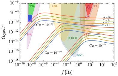
Figure 1: GW spectrum emitted from cosmic string loops. We take $G\mu=10^{-12}$, $10^{-16}$, and $10^{-20}$ (from top to bottom) with $N=2$ (blue), $5$ (yellow), $10$ (green), and $20$ (red). For the sensitivity curves and current constraint, see the main text.

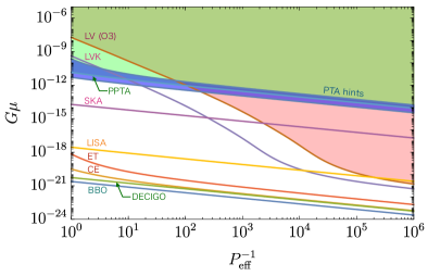
Figure 2: Sensitivity curves for ongoing and planned GW experiments in the $G\mu$-$P_{\rm eff}^{-1}$ plane. The green and red shaded regions are excluded by the current experiments. The blue shaded region is favored to explain the PTA hints.

V.1 Results

We numerically solve the extended VOS equations and calculate the GW spectrum, where we take $\Omega_{\Lambda}=0.685$ and $\Omega_{m}=0.315$ Planck:2018vyg as the cosmological parameters. We take into account the entropy production by decoupling the relativistic degrees of freedom in the Standard–Model sector. The resulting GW spectra are shown in Fig. 1 for the cases of $G\mu=10^{-12}$, $10^{-16}$, and $10^{-20}$ with $N=2,5,10$, and $20$. We take $\alpha=0.1$ and $N_{\rm scat}=10$. The peak amplitude of the GWs and the peak frequency are approximately given by

$$\left(\Omega_{\rm GW}h^{2}\right)^{(\rm peak)}\simeq 2.5\times 10^{-10}\times P_{\rm eff}^{-1}\left(\frac{G\mu}{10^{-12}}\right)^{1/2}\left(\frac{\alpha}{0.1}\right)^{1/2},$$ (17)

$$f^{(\rm peak)}\simeq 1.9\times 10^{-6}\times\left(\frac{G\mu}{10^{-12}}\right)^{-1},$$ (18)

for $\alpha\gg\Gamma G\mu$. Because the dependence of $P_{\rm eff}^{-1}$ and $G\mu$ are not degenerate, we can determine both by observing the spectra around the peaks.

We follow Ref. Schmitz:2020syl to plot the power-law-integrated sensitivity curves for ongoing and planned GW experiments: SKA Janssen:2014dka , LISA LISA:2017pwj , DECIGO Kawamura:2011zz ; Kawamura:2020pcg , BBO Harry:2006fi , Einstein Telescope (ET) Punturo:2010zz ; Maggiore:2019uih , Cosmic Explorer (CE) Reitze:2019iox , and aLIGO+aVirgo+KAGRA (LVK) Somiya:2011np ; KAGRA:2020cvd . The current constraints from the Parkes pulsar timing array (PPTA) Shannon:2015ect and aLIGO/aVirgo’s third observing run (LV(O3)) KAGRA:2021kbb are shown as green and red shaded regions, respectively. The blue box highlights the potential signals of pulsar timing array (PTA) experiments: NANOGrav NANOGrav:2020bcs and the PPTA Goncharov:2021oub . See Refs. Ellis:2020ena ; Blasi:2020mfx ; Blanco-Pillado:2021ygr for other cosmic string models to explain the PTA hints.

Figure 2 shows the sensitivity curves in the $G\mu$-$P_{\rm eff}^{-1}$ plane. The red and green shaded regions are excluded by the current experiments. The blue shaded region is favored to explain the PTA hints. Interestingly, we can predict the signals in LVK consistently with the PTA experiments for $P_{\rm eff}^{-1}\gtrsim 10$. This is because the peak amplitude can be enhanced without changing the peak frequency for a large $P_{\rm eff}^{-1}$.

We note that $\mu$ and $P_{\rm eff}$ can be interpreted as physical quantities $\Lambda$ and $N$ from Eqs. (10) and (11), with $\mathcal{O}(1)$ uncertainties. In particular, for the case of F-strings, GW signals can be observed for $\Lambda\gtrsim 10^{8}\ {\rm GeV}$ and $N=\mathcal{O}(1\,\text{-}\,10)$. For the case of D-strings, one should be careful about the exponentially suppressed intercommutation probability because it may become $\mathcal{O}(1)$ for $v\sim\mathcal{O}(1/N)$. Collisions with such a low relative velocity may not be negligible in the random motion of the cosmic string network. We do not further discuss this issue in this letter and leave it for a future work.

V.2 $\alpha$-dependence

Finally, we show the dependence of GW spectrum on the size of string loops $\alpha$. Figure 3 shows the GW spectrum for the case of $G\mu=10^{-12}$ and $P_{\rm eff}=0.1$ with $\alpha=10^{-1}$, $10^{-3}$, $10^{-5}$, $10^{-7}$, $10^{-9}$, $10^{-11}$, $10^{-13}$, and $10^{-15}$ from top left to bottom right. The red dashed curve represents the contour of the maximum of the spectrum, i.e., ($f^{(\rm peak)},\left(\Omega_{\rm GW}h^{2}\right)^{(\rm peak)}$), for $\alpha$ ranging from $10^{-1}$ to $10^{-15}$. As in the standard scenario of VOS model, the peak amplitude and frequency of GW spectrum depends on $\alpha$ such as $\left(\Omega_{\rm GW}h^{2}\right)^{(\rm peak)}\propto\alpha^{1/2}$ and $f^{(\rm peak)}\propto\alpha^{0}$ for $\alpha\gg\Gamma G\mu$ and $\left(\Omega_{\rm GW}h^{2}\right)^{(\rm peak)}\propto\alpha^{0}$ and $f^{(\rm peak)}\propto\alpha^{-1}$ for $\alpha\ll\Gamma G\mu$ (see, e.g., Ref. Auclair:2019wcv ). The numerical factors are determined by our numerical calculations and are given by Eqs. (17) and (18) for $\alpha\gg\Gamma G\mu$ and

$$\left(\Omega_{\rm GW}h^{2}\right)^{(\rm peak)}\simeq 3.8\times 10^{-14}\times P_{\rm eff}^{-1}\left(\frac{G\mu}{10^{-12}}\right),$$ (19)

$$f^{(\rm peak)}\simeq 5.2\times 10^{-7}\times\left(\frac{G\mu}{10^{-12}}\right)^{-1}\left(\frac{\alpha}{\Gamma G\mu}\right)^{-1},$$ (20)

for $\alpha\ll\Gamma G\mu$.

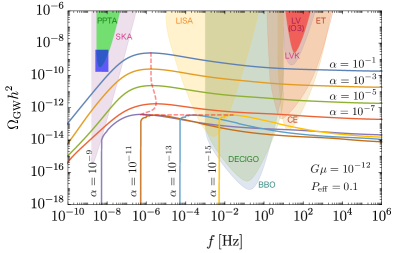
Figure 3: Same as Fig. 1 but with $G\mu=10^{-12}$ and $P_{\rm eff}=0.1$ for the case of $\alpha=10^{-1}$, $10^{-3}$, $10^{-5}$, $10^{-7}$, $10^{-9}$, $10^{-11}$, $10^{-13}$, and $10^{-15}$ from top left to bottom right. The red dashed curve represents the contour of the maximum of the spectrum, i.e., ($f^{(\rm peak)},\left(\Omega_{\rm GW}h^{2}\right)^{(\rm peak)}$), for $\alpha$ ranging from $10^{-1}$ to $10^{-15}$.

As $\alpha$ decreases from a relatively large value and approaches to $\Gamma G\mu$, the peak frequency slightly increases, decreases, and then increases again. This is in contrast to the case with the standard scenario of VOS model, where the peak frequency slightly decreases and then increases Sanidas:2012ee . This is because the last term in Eq. (12) is modified in the extended VOS model, which then leads to a different behavior on the $\alpha$ dependence around $\alpha\sim\Gamma G\mu$. However, the difference is not significant or important for our purpose.

For the case of $\alpha\ll\Gamma G\mu$, the spectrum has a lower cutoff on the frequency and is oscillating around the cutoff. This is because the contribution to the summation of Eq. (16) comes only from $n=1$ just above the cutoff and higher modes come into the contribution as the frequency increases. Since $n$ must be integer and each modes contributes with a similar order of magnitude, the spectrum increases discretely as the frequency increases.

Figure 4 shows the sensitivity curves in the $G\mu$-$\alpha$ plane. We take $P_{\rm eff}=1$, $10^{-1}$, $10^{-3}$, and $10^{-5}$ from top to bottom. The dashed line represents the value at $\alpha=\Gamma G\mu$. Because of the different parameter dependence of the GW spectrum for $\alpha\gg\Gamma G\mu$ and $\alpha\ll\Gamma G\mu$, the sensitivity curves have different behavior for those limits. If we adopt $\alpha\sim\Gamma G\mu$ rather than $\alpha=0.1$, the sensitivity on $G\mu$ by LISA is weakened by a factor of $\mathcal{O}(10^{-6})$ for the case of $P_{\rm eff}=\mathcal{O}(0.1)$, whereas it is $\mathcal{O}(10^{-3})$ for the case of $P_{\rm eff}=\mathcal{O}(10^{-5})$.

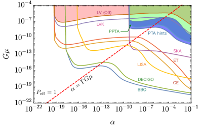
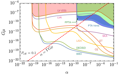
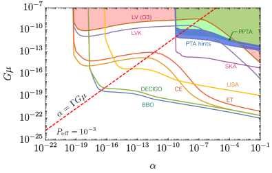
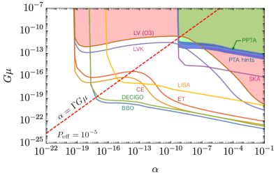
Figure 4: Same as Fig. 2 but with $P_{\rm eff}=1$, $10^{-1}$, $10^{-3}$, and $10^{-5}$ (from top to bottom)) in the $G\mu$-$\alpha$ plane. The dashed line represents $\alpha=\Gamma G\mu$.

VI Discussion and conclusions

We have discussed the formation and properties of macroscopic color flux tubes or cosmic strings in pure YM theories, such as SU($N$), Sp($N$), and SO($N$), and calculated their GW signals. These cosmic strings have a small intercommutation probability for a large $N$, just like cosmic superstrings; however, we do not assume a brane inflationary scenario or extra dimensions. The resulting GW signals can be observed by some ongoing and planned GW experiments if the dynamical scale is $\mathcal{O}(10^{8\,\text{-}\,13})\ {\rm GeV}$ for $N=\mathcal{O}(1\,\text{-}\,10)$ and $\alpha=0.1$. We also clarify how the GW spectrum changes for a smaller loop size $\alpha$.

We have considered the case with a single type of cosmic strings without a baryon vertex to calculate GW signals. The $\mathrm{SO}(N)$ gauge theory may contain F-strings as well as D-strings. The tensions and intercommutation probabilities of these cosmic strings have different dependence on $N$ for a large $N$. The dynamics of the network can be described by introducing a VOS equation for each string with transition terms Avgoustidis:2007aa . The effect of a baryon vertex, such as in the case of $\mathrm{SU}(N)$ with $N\geq 3$, is not fully understood particularly for a large $N$. We expect that baryon vertices form after the phase transition and their number density should also have a scaling behavior. We leave these topics for a future work, as detailed numerical simulations may be necessary.

In previous studies, the YM theory with the deconfinement/confinement phase transition has been extensively considered for the formation of glueballs Morningstar:1999rf ; Lucini:2010nv ; Curtin:2022tou , which is a candidate for dark matter Faraggi:2000pv ; Feng:2011ik ; Boddy:2014yra ; Boddy:2014qxa ; Soni:2016gzf ; Kribs:2016cew ; Forestell:2016qhc ; Soni:2017nlm ; Forestell:2017wov ; Jo:2020ggs . Our results suggest that such a scenario inevitably results in the formation of F- and/or D-strings and predicts GW signals from string loops. However, these glueballs may decay before the big-bang nucleosynthesis epoch in the case of $\Lambda\gtrsim 10^{8}\ {\rm GeV}$ Juknevich:2009ji ; Juknevich:2009gg ; Halverson:2016nfq ; Asadi:2022vkc , which is the parameter of our interest.

We note that we only assume that the phase transition occurs after inflation. In particular, the phase transition can occur during an inflation—oscillation-dominated era. Even in this case, our result does not change because the GWs are emitted from string loops in the scaling regime of the RD. For the same reason, our calculation does not change even if the temperature of the gauge sector is different from that of the Standard–Model sector.

- (1) R. Bousso and J. Polchinski, Quantization of four form fluxes and dynamical neutralization of the cosmological constant, JHEP 06 (2000) 006 [hep-th/0004134].
- (2) L. Susskind, The Anthropic landscape of string theory, hep-th/0302219.
- (3) E. Witten, Some Properties of O(32) Superstrings, Phys. Lett. B 149 (1984) 351.
- (4) P. Svrcek and E. Witten, Axions In String Theory, JHEP 06 (2006) 051 [hep-th/0605206].
- (5) A. Arvanitaki, S. Dimopoulos, S. Dubovsky, N. Kaloper and J. March-Russell, String Axiverse, Phys. Rev. D 81 (2010) 123530 [0905.4720].
- (6) C. Vafa, The String landscape and the swampland, hep-th/0509212.
- (7) N. Arkani-Hamed, L. Motl, A. Nicolis and C. Vafa, The String landscape, black holes and gravity as the weakest force, JHEP 06 (2007) 060 [hep-th/0601001].
- (8) S. K. Garg and C. Krishnan, Bounds on Slow Roll and the de Sitter Swampland, JHEP 11 (2019) 075 [1807.05193].
- (9) H. Ooguri, E. Palti, G. Shiu and C. Vafa, Distance and de Sitter Conjectures on the Swampland, Phys. Lett. B 788 (2019) 180 [1810.05506].
- (10) G. R. Dvali and S. H. H. Tye, Brane inflation, Phys. Lett. B 450 (1999) 72 [hep-ph/9812483].
- (11) G. Dvali and A. Vilenkin, Formation and evolution of cosmic D strings, JCAP 03 (2004) 010 [hep-th/0312007].
- (12) E. J. Copeland, R. C. Myers and J. Polchinski, Cosmic F and D strings, JHEP 06 (2004) 013 [hep-th/0312067].
- (13) N. T. Jones, H. Stoica and S. H. H. Tye, The Production, spectrum and evolution of cosmic strings in brane inflation, Phys. Lett. B 563 (2003) 6 [hep-th/0303269].
- (14) M. G. Jackson, N. T. Jones and J. Polchinski, Collisions of cosmic F and D-strings, JHEP 10 (2005) 013 [hep-th/0405229].
- (15) A. Vilenkin, Gravitational radiation from cosmic strings, Phys. Lett. B 107 (1981) 47.
- (16) T. Vachaspati and A. Vilenkin, Gravitational Radiation from Cosmic Strings, Phys. Rev. D 31 (1985) 3052.
- (17) J. Polchinski, Collision of Macroscopic Fundamental Strings, Phys. Lett. B 209 (1988) 252.
- (18) A. Hanany and K. Hashimoto, Reconnection of colliding cosmic strings, JHEP 06 (2005) 021 [hep-th/0501031].
- (19) T. W. B. Kibble, Evolution of a system of cosmic strings, Nucl. Phys. B 252 (1985) 227.
- (20) C. J. A. P. Martins and E. P. S. Shellard, String evolution with friction, Phys. Rev. D 53 (1996) 575 [hep-ph/9507335].
- (21) C. J. A. P. Martins and E. P. S. Shellard, Quantitative string evolution, Phys. Rev. D 54 (1996) 2535 [hep-ph/9602271].
- (22) C. J. A. P. Martins and E. P. S. Shellard, Extending the velocity dependent one scale string evolution model, Phys. Rev. D 65 (2002) 043514 [hep-ph/0003298].
- (23) C. Ringeval, M. Sakellariadou and F. Bouchet, Cosmological evolution of cosmic string loops, JCAP 02 (2007) 023 [astro-ph/0511646].
- (24) J. J. Blanco-Pillado, K. D. Olum and B. Shlaer, Large parallel cosmic string simulations: New results on loop production, Phys. Rev. D 83 (2011) 083514 [1101.5173].
- (25) J. J. Blanco-Pillado, K. D. Olum and B. Shlaer, The number of cosmic string loops, Phys. Rev. D 89 (2014) 023512 [1309.6637].
- (26) J. J. Blanco-Pillado and K. D. Olum, Stochastic gravitational wave background from smoothed cosmic string loops, Phys. Rev. D 96 (2017) 104046 [1709.02693].
- (27) J. J. Blanco-Pillado, K. D. Olum and X. Siemens, New limits on cosmic strings from gravitational wave observation, Phys. Lett. B 778 (2018) 392 [1709.02434].
- (28) R. R. Caldwell and B. Allen, Cosmological constraints on cosmic string gravitational radiation, Phys. Rev. D 45 (1992) 3447.
- (29) M. R. DePies and C. J. Hogan, Stochastic Gravitational Wave Background from Light Cosmic Strings, Phys. Rev. D 75 (2007) 125006 [astro-ph/0702335].
- (30) S. A. Sanidas, R. A. Battye and B. W. Stappers, Constraints on cosmic string tension imposed by the limit on the stochastic gravitational wave background from the European Pulsar Timing Array, Phys. Rev. D 85 (2012) 122003 [1201.2419].
- (31) L. Sousa and P. P. Avelino, Stochastic Gravitational Wave Background generated by Cosmic String Networks: Velocity-Dependent One-Scale model versus Scale-Invariant Evolution, Phys. Rev. D 88 (2013) 023516 [1304.2445].
- (32) L. Sousa and P. P. Avelino, Probing Cosmic Superstrings with Gravitational Waves, Phys. Rev. D 94 (2016) 063529 [1606.05585].
- (33) A. Avgoustidis and E. P. S. Shellard, Effect of reconnection probability on cosmic (super)string network density, Phys. Rev. D 73 (2006) 041301 [astro-ph/0512582].
- (34) M. Yamada and K. Yonekura, Cosmic strings from pure Yang-Mills theory, 2204.13123.
- (35) N. Seiberg and E. Witten, Electric - magnetic duality, monopole condensation, and confinement in N=2 supersymmetric Yang-Mills theory, Nucl. Phys. B 426 (1994) 19 [hep-th/9407087].
- (36) A. Athenodorou and M. Teper, SU(N) gauge theories in 3+1 dimensions: glueball spectrum, string tensions and topology, JHEP 12 (2021) 082 [2106.00364].
- (37) G. ’t Hooft, A Planar Diagram Theory for Strong Interactions, Nucl. Phys. B 72 (1974) 461.
- (38) S. Coleman, Aspects of Symmetry: Selected Erice Lectures. Cambridge University Press, Cambridge, U.K., 1985, 10.1017/CBO9780511565045.
- (39) E. Witten, Anti-de Sitter space, thermal phase transition, and confinement in gauge theories, Adv. Theor. Math. Phys. 2 (1998) 505 [hep-th/9803131].
- (40) J. Polchinski and M. J. Strassler, The String dual of a confining four-dimensional gauge theory, hep-th/0003136.
- (41) I. R. Klebanov and M. J. Strassler, Supergravity and a confining gauge theory: Duality cascades and chi SB resolution of naked singularities, JHEP 08 (2000) 052 [hep-th/0007191].
- (42) J. M. Maldacena and C. Nunez, Towards the large N limit of pure N=1 superYang-Mills, Phys. Rev. Lett. 86 (2001) 588 [hep-th/0008001].
- (43) C. Vafa, Superstrings and topological strings at large N, J. Math. Phys. 42 (2001) 2798 [hep-th/0008142].
- (44) A. Vilenkin, COSMOLOGICAL EVOLUTION OF MONOPOLES CONNECTED BY STRINGS, Nucl. Phys. B 196 (1982) 240.
- (45) M. A. Luty and T. Okui, Conformal technicolor, JHEP 09 (2006) 070 [hep-ph/0409274].
- (46) M. Ibe, Y. Nakayama and T. T. Yanagida, Conformal Gauge Mediation, Phys. Lett. B 649 (2007) 292 [hep-ph/0703110].
- (47) T. T. Yanagida and K. Yonekura, A Conformal Gauge Mediation and Dark Matter with Only One Parameter, Phys. Lett. B 693 (2010) 281 [1006.2271].
- (48) W. Buchmuller, V. Domcke and K. Schmitz, Stochastic gravitational-wave background from metastable cosmic strings, JCAP 12 (2021) 006 [2107.04578].
- (49) D. I. Dunsky, A. Ghoshal, H. Murayama, Y. Sakakihara and G. White, Gravitational Wave Gastronomy, 2111.08750.
- (50) G. Lazarides, R. Maji and Q. Shafi, Gravitational Waves from Quasi-stable Strings, 2203.11204.
- (51) D. Gaiotto, A. Kapustin, N. Seiberg and B. Willett, Generalized Global Symmetries, JHEP 02 (2015) 172 [1412.5148].
- (52) G. ’t Hooft, On the Phase Transition Towards Permanent Quark Confinement, Nucl. Phys. B 138 (1978) 1.
- (53) G. ’t Hooft, A Property of Electric and Magnetic Flux in Nonabelian Gauge Theories, Nucl. Phys. B 153 (1979) 141.
- (54) E. Witten, Cosmic Superstrings, Phys. Lett. B 153 (1985) 243.
- (55) T. Vachaspati and A. Vilenkin, Evolution of cosmic networks, Phys. Rev. D 35 (1987) 1131.
- (56) M. Hindmarsh and T. W. B. Kibble, BEADS ON STRINGS, Phys. Rev. Lett. 55 (1985) 2398.
- (57) V. Berezinsky and A. Vilenkin, Cosmic necklaces and ultrahigh-energy cosmic rays, Phys. Rev. Lett. 79 (1997) 5202 [astro-ph/9704257].
- (58) M. Hindmarsh, K. Rummukainen and D. J. Weir, Numerical simulations of necklaces in SU(2) gauge-Higgs field theory, Phys. Rev. D 95 (2017) 063520 [1611.08456].
- (59) E. J. Copeland and P. M. Saffin, On the evolution of cosmic-superstring networks, JHEP 11 (2005) 023 [hep-th/0505110].
- (60) M. Hindmarsh and P. M. Saffin, Scaling in a SU(2) model of cosmic superstring networks, JHEP 08 (2006) 066 [hep-th/0605014].
- (61) J. Urrestilla and A. Vilenkin, Evolution of cosmic superstring networks: A Numerical simulation, JHEP 02 (2008) 037 [0712.1146].
- (62) E. Witten, Baryons in the 1/n Expansion, Nucl. Phys. B 160 (1979) 57.
- (63) E. Witten, Baryons and branes in anti-de Sitter space, JHEP 07 (1998) 006 [hep-th/9805112].
- (64) N. T. Jones, H. Stoica and S. H. H. Tye, Brane interaction as the origin of inflation, JHEP 07 (2002) 051 [hep-th/0203163].
- (65) S. Sarangi and S. H. H. Tye, Cosmic string production towards the end of brane inflation, Phys. Lett. B 536 (2002) 185 [hep-th/0204074].
- (66) G. Dvali and A. Vilenkin, Solitonic D-branes and brane annihilation, Phys. Rev. D 67 (2003) 046002 [hep-th/0209217].
- (67) L. Pogosian, S. H. H. Tye, I. Wasserman and M. Wyman, Observational constraints on cosmic string production during brane inflation, Phys. Rev. D 68 (2003) 023506 [hep-th/0304188].
- (68) C. J. A. P. Martins and E. P. S. Shellard, Fractal properties and small-scale structure of cosmic string networks, Phys. Rev. D 73 (2006) 043515 [astro-ph/0511792].
- (69) M. Sakellariadou, A Note on the evolution of cosmic string/superstring networks, JCAP 04 (2005) 003 [hep-th/0410234].
- (70) C. J. A. P. Martins, J. N. Moore and E. P. S. Shellard, A Unified model for vortex string network evolution, Phys. Rev. Lett. 92 (2004) 251601 [hep-ph/0310255].
- (71) D. P. Bennett and F. R. Bouchet, High resolution simulations of cosmic string evolution. 1. Network evolution, Phys. Rev. D 41 (1990) 2408.
- (72) B. Allen and E. P. S. Shellard, Cosmic string evolution: a numerical simulation, Phys. Rev. Lett. 64 (1990) 119.
- (73) M. Sakellariadou and A. Vilenkin, Cosmic-string evolution in flat space-time, Phys. Rev. D 42 (1990) 349.
- (74) C. J. Burden, Gravitational Radiation From a Particular Class of Cosmic Strings, Phys. Lett. B 164 (1985) 277.
- (75) D. Garfinkle and T. Vachaspati, Radiation From Kinky, Cuspless Cosmic Loops, Phys. Rev. D 36 (1987) 2229.
- (76) A. Vilenkin and E. P. S. Shellard, Cosmic Strings and Other Topological Defects. Cambridge University Press, 7, 2000.
- (77) Planck collaboration, N. Aghanim et al., Planck 2018 results. VI. Cosmological parameters, Astron. Astrophys. 641 (2020) A6 [1807.06209].
- (78) K. Schmitz, New Sensitivity Curves for Gravitational-Wave Signals from Cosmological Phase Transitions, JHEP 01 (2021) 097 [2002.04615].
- (79) G. Janssen et al., Gravitational wave astronomy with the SKA, PoS AASKA14 (2015) 037 [1501.00127].
- (80) LISA collaboration, P. Amaro-Seoane et al., Laser Interferometer Space Antenna, 1702.00786.
- (81) S. Kawamura et al., The Japanese space gravitational wave antenna: DECIGO, Class. Quant. Grav. 28 (2011) 094011.
- (82) S. Kawamura et al., Current status of space gravitational wave antenna DECIGO and B-DECIGO, PTEP 2021 (2021) 05A105 [2006.13545].
- (83) G. M. Harry, P. Fritschel, D. A. Shaddock, W. Folkner and E. S. Phinney, Laser interferometry for the big bang observer, Class. Quant. Grav. 23 (2006) 4887.
- (84) M. Punturo et al., The Einstein Telescope: A third-generation gravitational wave observatory, Class. Quant. Grav. 27 (2010) 194002.
- (85) M. Maggiore et al., Science Case for the Einstein Telescope, JCAP 03 (2020) 050 [1912.02622].
- (86) D. Reitze et al., Cosmic Explorer: The U.S. Contribution to Gravitational-Wave Astronomy beyond LIGO, Bull. Am. Astron. Soc. 51 (2019) 035 [1907.04833].
- (87) KAGRA collaboration, K. Somiya, Detector configuration of KAGRA: The Japanese cryogenic gravitational-wave detector, Class. Quant. Grav. 29 (2012) 124007 [1111.7185].
- (88) KAGRA collaboration, T. Akutsu et al., Overview of KAGRA : KAGRA science, 2008.02921.
- (89) R. M. Shannon et al., Gravitational waves from binary supermassive black holes missing in pulsar observations, Science 349 (2015) 1522 [1509.07320].
- (90) KAGRA, Virgo, LIGO Scientific collaboration, R. Abbott et al., Upper limits on the isotropic gravitational-wave background from Advanced LIGO and Advanced Virgo’s third observing run, Phys. Rev. D 104 (2021) 022004 [2101.12130].
- (91) NANOGrav collaboration, Z. Arzoumanian et al., The NANOGrav 12.5 yr Data Set: Search for an Isotropic Stochastic Gravitational-wave Background, Astrophys. J. Lett. 905 (2020) L34 [2009.04496].
- (92) B. Goncharov et al., On the Evidence for a Common-spectrum Process in the Search for the Nanohertz Gravitational-wave Background with the Parkes Pulsar Timing Array, Astrophys. J. Lett. 917 (2021) L19 [2107.12112].
- (93) J. Ellis and M. Lewicki, Cosmic String Interpretation of NANOGrav Pulsar Timing Data, Phys. Rev. Lett. 126 (2021) 041304 [2009.06555].
- (94) S. Blasi, V. Brdar and K. Schmitz, Has NANOGrav found first evidence for cosmic strings?, Phys. Rev. Lett. 126 (2021) 041305 [2009.06607].
- (95) J. J. Blanco-Pillado, K. D. Olum and J. M. Wachter, Comparison of cosmic string and superstring models to NANOGrav 12.5-year results, Phys. Rev. D 103 (2021) 103512 [2102.08194].
- (96) P. Auclair et al., Probing the gravitational wave background from cosmic strings with LISA, JCAP 04 (2020) 034 [1909.00819].
- (97) A. Avgoustidis and E. P. S. Shellard, Velocity-Dependent Models for Non-Abelian/Entangled String Networks, Phys. Rev. D 78 (2008) 103510 [0705.3395].
- (98) C. J. Morningstar and M. J. Peardon, The Glueball spectrum from an anisotropic lattice study, Phys. Rev. D 60 (1999) 034509 [hep-lat/9901004].
- (99) B. Lucini, A. Rago and E. Rinaldi, Glueball masses in the large N limit, JHEP 08 (2010) 119 [1007.3879].
- (100) D. Curtin, C. Gemmell and C. B. Verhaaren, Simulating Glueball Production in QCD, 2202.12899.
- (101) A. E. Faraggi and M. Pospelov, Selfinteracting dark matter from the hidden heterotic string sector, Astropart. Phys. 16 (2002) 451 [hep-ph/0008223].
- (102) J. L. Feng and Y. Shadmi, WIMPless Dark Matter from Non-Abelian Hidden Sectors with Anomaly-Mediated Supersymmetry Breaking, Phys. Rev. D 83 (2011) 095011 [1102.0282].
- (103) K. K. Boddy, J. L. Feng, M. Kaplinghat and T. M. P. Tait, Self-Interacting Dark Matter from a Non-Abelian Hidden Sector, Phys. Rev. D 89 (2014) 115017 [1402.3629].
- (104) K. K. Boddy, J. L. Feng, M. Kaplinghat, Y. Shadmi and T. M. P. Tait, Strongly interacting dark matter: Self-interactions and keV lines, Phys. Rev. D 90 (2014) 095016 [1408.6532].
- (105) A. Soni and Y. Zhang, Hidden SU(N) Glueball Dark Matter, Phys. Rev. D 93 (2016) 115025 [1602.00714].
- (106) G. D. Kribs and E. T. Neil, Review of strongly-coupled composite dark matter models and lattice simulations, Int. J. Mod. Phys. A 31 (2016) 1643004 [1604.04627].
- (107) L. Forestell, D. E. Morrissey and K. Sigurdson, Non-Abelian Dark Forces and the Relic Densities of Dark Glueballs, Phys. Rev. D 95 (2017) 015032 [1605.08048].
- (108) A. Soni, H. Xiao and Y. Zhang, Cosmic selection rule for the glueball dark matter relic density, Phys. Rev. D 96 (2017) 083514 [1704.02347].
- (109) L. Forestell, D. E. Morrissey and K. Sigurdson, Cosmological Bounds on Non-Abelian Dark Forces, Phys. Rev. D 97 (2018) 075029 [1710.06447].
- (110) B. Jo, H. Kim, H. D. Kim and C. S. Shin, Exploring the Universe with dark light scalars, Phys. Rev. D 103 (2021) 083528 [2010.10880].
- (111) J. E. Juknevich, D. Melnikov and M. J. Strassler, A Pure-Glue Hidden Valley I. States and Decays, JHEP 07 (2009) 055 [0903.0883].
- (112) J. E. Juknevich, Pure-glue hidden valleys through the Higgs portal, JHEP 08 (2010) 121 [0911.5616].
- (113) J. Halverson, B. D. Nelson and F. Ruehle, String Theory and the Dark Glueball Problem, Phys. Rev. D 95 (2017) 043527 [1609.02151].
- (114) P. Asadi, E. D. Kramer, E. Kuflik, T. R. Slatyer and J. Smirnov, Glueballs in a Thermal Squeezeout Model, 2203.15813.