TU-1152

Cosmic strings from pure Yang–Mills theory

Masaki Yamada^1,2 and Kazuya Yonekura¹

1 Department of Physics, Tohoku University, Sendai 980-8578, Japan

2 FRIS, Tohoku University, Sendai, Miyagi 980-8578, Japan

We discuss the formation of cosmic strings or macroscopic color flux tubes at the phase transition from the deconfinement to confinement phase in pure Yang–Mills (YM) theory, such as $\mathrm{SU}(N)$, $\mathrm{Sp}(N)$, $\mathrm{SO}(N)$, and $\mathrm{Spin}(N)$, based on the current understanding of theoretical physics. According to the holographic dual descriptions, the cosmic strings are dual to fundamental strings or wrapped D-branes in the gravity side depending on the structure of the gauge group, and the reconnection probability is suppressed by $\mathcal{O}(N^{-2})$ and $e^{-\mathcal{O}(N)}$, respectively. The pure YM theory thus provides a simple realization of cosmic F- and D-strings without the need for a brane-inflationary scenario or extra dimension. We also review the stability of cosmic strings based on the concept of 1-form symmetry, which further implies the existence of a baryon vertex in some YM theory. We calculate the gravitational wave spectrum that is emitted from the cosmic strings based on an extended velocity-dependent one-scale model and discuss its detectability based on ongoing and planned gravitational-wave experiments. In particular, the SKA and LISA can observe gravitational signals if the confinement scale is higher than $\mathcal{O}(10^{12})\,\mathrm{GeV}$ and $\mathcal{O}(10^{10})\,\mathrm{GeV}$ for $\mathrm{SU}(N)$ with $N=\mathcal{O}(1)$, respectively.

1 Introduction

The strong dynamics of gauge theory is an important topic in theoretical physics; it helps understand the nature of mesons and baryons in QCD. The Universe is characterized as a unique application domain or system because it is cooled down from a very high temperature wherein the gauge theory is weakly coupled. The deconfinement/confinement phase transition should have occurred at a certain period of time in the cosmological history, which provides a rich phenomenology in cosmology. For instance, even an $\mathrm{SU}(N)$ Yang–Mills (YM) theory with or without a quark that is heavier than the confinement scale is extensively considered in the literature [1, 2, 3, 4]. Further, glueballs are formed at the deconfinement/confinement phase transition [5, 6, 7]. The glueballs can be dark matter (DM) if their lifetime is sufficiently long  [8, 9, 10, 11, 12, 13, 14, 15, 16, 17]. They can also be self-interacting DM that may address the problems of small-scale structure in cosmology [18, 19]. The overproduction problem and decay of glueballs are considered in Ref. [20, 21, 22, 23]. The gravitational wave (GW) signals from the first-order phase transition has also been investigated [24].

In this paper, we demonstrate that cosmic strings or macroscopic color flux tubes form at the phase transition of pure YM theory from the deconfinement to the confinement phase. We explain the generalized symmetry or higher-form symmetry [25] that ensures the stability of topological objects, including the cosmic strings in the pure YM theory. This concept is a generalization of ordinal (0-form) symmetry that ensures the stability of a (0-dimensional) particle. One-form symmetry ensures the stability of cosmic strings that are one-dimensional objects. For example, the pure $\mathrm{SU}(N)$ gauge theory has discrete one-form symmetry, which is referred to as ${\mathbb{Z}}_{N}^{[1]}$. This implies the existence of one-dimensional objects charged under ${\mathbb{Z}}_{N}^{[1]}$. It is further identified as the color flux tube in the confinement phase. Such color flux tubes should form at the deconfinement/confinement phase transition with a cosmological scale, and they can be regarded as cosmic strings. ${\mathbb{Z}}_{N}^{[1]}$ symmetry implies that $N$ strings can joined at a vertex, referred to as a baryon vertex. This is similar to the ${\mathbb{Z}}_{N}$-string, which is considered in field-theory models [29]. However, our cosmic strings are qualitatively different from those produced in weakly coupled field-theory models, and we will provide a detailed explanation in the forthcoming sections. In some gauge groups, such as $\mathrm{Sp}(N)$, the one-form symmetry is ${\mathbb{Z}}_{2}^{[1]}$ for any $N$ and the baryon vertex, even if it exists, does not play a significant role in cosmology.

We also discuss some other properties of cosmic strings in pure YM theory according to electric–magnetic duality, large $N$ limit, and holographic dual descriptions. The electric–magnetic duality implies that the confinement is dual to Higgsing [30], such that the cosmic strings should form at the phase transition similar to the case where a $\mathrm{U}(1)$ symmetry is spontaneously broken in weakly coupled field-theory models. The reconnection probability of cosmic strings can be estimated in the large $N$ limit such as $1/N^{2}$ for $\mathrm{SU}(N)$ [31] (see Ref. [32] for a review). According to the holographic dual descriptions, the cosmic strings are dual to a fundamental string or a wrapped D-brane in the gravity side depending on the structure of the gauge group (see, e.g., Refs. [33, 34, 35, 36, 37]). We refer to these as F-string and D-string, respectively. The reconnection probability scales as $1/N^{2}$ for F-strings and $e^{-\mathcal{O}(1)}$ for D-strings, which is consistent with the argument of the large $N$ limit. The suppressed reconnection probability is similar to that of the cosmic superstrings that form after the brane inflationary scenario [38, 39]. In our case, however, the brane inflation is not required. The pure YM theory provides a cosmic string with a small reconnection probability using a simple setup.

Cosmic strings can be indirectly detected by observing GWs emitted from stochastic dynamics [40, 41]. We calculate the GW spectrum that is emitted from string loops with a small reconnection (or intercommutation) probability. The cosmic string network can be described by extending the velocity-dependent one-scale (VOS) model [42, 43, 44, 45] to consider the small intercommutation probability. The extended VOS model was originally proposed in Ref. [46], where they also confirm its consistency with numerical simulations. The resulting GW signal can be within the reach of the future sensitivity of the Square Kilometer Array (SKA) [47] and LISA [48] if the confinement scale $\Lambda$ is higher than $\mathcal{O}(10^{12})$ and $\mathcal{O}(10^{10})$, respectively. We can determine the $N$ and the confinement scale $\Lambda$ by observing the GW spectrum.

The rest of this paper is organized as follows. In Sec. 2, we review the idea of 1-form symmetries. This topic has attracted significant attention in theoretical physics and is also important for particle cosmology that treats topological defects and (pseudo-) NG modes (see, e.g., Refs. [49, 50, 51, 52, 53, 54, 55, 56, 57]). We particularly show that the pure $\mathrm{SU}(N)$ gauge theory has a 1-form ${\mathbb{Z}}_{N}^{[1]}$ symmetry under which the color flux tube or cosmic string is charged. In Sec. 3, we use other theoretical tools to demonstrate the properties of cosmic strings in the pure YM theory. Based on the electric–magnetic duality, we expect that the cosmic strings form at the deconfinement/confinement phase transition, similar to the formation of cosmic strings in ordinal field-theory models with a spontaneously broken $\mathrm{U}(1)$ symmetry. In the large $N$ limit, we explain that the intercommutation probability should scale as $1/N^{2}$ for $\mathrm{SU}(N)$. Such a small intercommutation probability is consistent with the holographic dual descriptions because cosmic strings can be identified as fundamental strings in the gravity side. We also discuss the differences for other gauge groups, such as $\mathrm{Sp}(N)$, $\mathrm{SO}(N)$, and $\mathrm{Spin}(N)$. In Sec. 4, we first summarize the properties of strings and qualitatively discuss the phenomenological consequence. We then solve the dynamics of long strings based on the extended VOS model. In Sec. 5, we calculate the GW spectrum that is emitted from cosmic string loops. The resulting spectrum is shown with the future sensitivity curves, including SKA and LISA. Sec. 6 comprises the discussion and conclusions of the paper.

2 Cosmic strings and 1-form symmetries

The stability of a particle can be guaranteed by considering the specific symmetry under which the particle is charged. For example, the stability of dark matter candidates can be ensured by introducing (global or gauge) symmetries such as ${\mathbb{Z}}_{N}$ or $\mathrm{U}(1)$. In the same way, the stability of a (cosmic) string can be ensured by 1-form symmetries [25]. We review this concept in this section. In the next section, we discuss some qualitative properties of color flux tubes in gauge theories. If the reader is interested only in the phenomenology of cosmic strings in the pure YM theory, she/he may skip the next two sections and directly refer to Section 4.

2.1 1-form symmetries and operators

In this section, we review the concept of 1-form symmetries in the operator formalism with a fixed time direction. We particularly consider operators that act on the Hilbert space. The study in [25] provides the general spacetime descriptions with time-ordered operators or in the Euclidean signature spacetime wherein the time direction need not be assumed. In the following discussions, we do not consider time ordering unless otherwise stated.

First, we recall how an ordinary $\mathrm{U}(1)$ symmetry can be described. We have the corresponding conserved Noether current $J^{\mu}$. Through the integration of this term, we obtain a conserved charge operator

$$Q(\Sigma)=\int_{\Sigma}d\Sigma_{\mu}J^{\mu}$$ (2.1)

where $\Sigma$ is a 3-dimensional surface inside the 4-dimensional spacetime such as the constant time slice $\Sigma=\{t={\rm const.}\}$, and $d\Sigma_{\mu}$ is set such that its length is the volume element of $\Sigma$ and its direction is orthogonal to the surface $\Sigma$. The conservation equation $\nabla_{\mu}J^{\mu}=0$ ensures that the charge operator $Q(\Sigma)$ depends only on the topology of $\Sigma$, and thus, it is invariant under a continuous change in $\Sigma$. This topological invariance is the abstract description of the usual charge conservation. For example, the topological invariance states that when we take two time slices $\Sigma_{1}=\{t=t_{1}\}$ and $\Sigma_{2}=\{t=t_{2}\}$, we obtain $Q(\Sigma_{1})=Q(\Sigma_{2})$ with the assumption that there is no flux of charge at spatial infinity.

Using the charge operator $Q(\Sigma)$, we can construct a unitary operator $U(\Sigma,\alpha)$ as

$$U(\Sigma,\alpha)=\exp[i\alpha Q(\Sigma)],$$ (2.2)

where $\alpha$ is an arbitrary parameter. This operator induces the symmetry transformation as follows. If ${\cal O}(x)$ is an operator whose charge is $q$ under the $\mathrm{U}(1)$, and if $\Sigma$ is topologicaly equivalent to a time slice $\Sigma=\{t={\rm const.}\}$, then we get

$$U(\Sigma,\alpha){\cal O}(x)U(\Sigma,\alpha)^{\dagger}=e^{iq\alpha}{\cal O}(x).$$ (2.3)

When the symmetry is not $\mathrm{U}(1)$ but a discrete group such as ${\mathbb{Z}}_{N}$, the current $J^{\mu}$ and the charge $Q(\Sigma)$ are not conserved. However, the unitary operator $U(\Sigma,\alpha)$ still persists, and it possesses the desired topological invariance related to $\Sigma$ provided that the parameter $\alpha$ is considered as $\alpha=2\pi k/N$, where $k\in{\mathbb{Z}}_{N}$. Thus, we can characterize the symmetry using such operators $U(\Sigma,\alpha)$. (See [25] for a complete description.)

Now, we can extend the aforementioned discussions to 1-form symmetries. First, let us consider a 1-form $\mathrm{U}(1)$ symmetry, which may be denoted as $\mathrm{U}(1)^{[1]}$. This symmetry is characterized by a current operator $J^{\mu\nu}$, which is antisymmetric $J^{\mu\nu}=-J^{\nu\mu}$; it is conserved in the sense that $\nabla_{\mu}J^{\mu\nu}=0$. We will discuss an explicit example later. The charge $Q(\Sigma)$ is defined as

$$Q(\Sigma)=\int_{\Sigma}\frac{1}{2}d\Sigma_{\mu\nu}J^{\mu\nu},$$ (2.4)

where $\Sigma$ is now a 2-dimensional surface, and $d\Sigma_{\mu\nu}$ is such that it is antisymmetric $d\Sigma_{\mu\nu}=-d\Sigma_{\nu\mu}$, its length $\sqrt{\frac{1}{2}d\Sigma_{\mu\nu}d\Sigma^{\mu\nu}}$ is the volume element of $\Sigma$, and its directions are orthogonal to $\Sigma$. (We conveniently define a 2-form $J=\frac{1}{2^{2}}\epsilon_{\mu\nu\rho\sigma}J^{\mu\nu}dx^{\rho}\wedge dx^{\sigma}$ using differential forms, and then $Q(\Sigma)=\int_{\Sigma}J$.) Based on the conservation equation $\nabla_{\mu}J^{\mu\nu}=0$ (or $dJ=0$ in the differential form notation), this operator depends only on the topology of $\Sigma$. More precisely, if we have two surfaces $\Sigma_{1}$ and $\Sigma_{2}$ such that there exists a 3-dimensional surface $\Gamma$ whose boundary is $\partial\Gamma=\Sigma_{1}-\Sigma_{2}$, we obtain $Q(\Sigma_{1})=Q(\Sigma_{2})$ (since $Q(\Sigma_{1})-Q(\Sigma_{2})=\int_{\Gamma}dJ=0$ using the Stokes theorem and the conservation equation $dJ=0$). In particular, $Q(\Sigma)$ is invariant under the continuous change of $\Sigma$.

We can also define $U(\Sigma,\alpha)=\exp[i\alpha Q(\Sigma)]$ similar to the case of ordinary symmetries. Now, in the case of ordinary symmetries, point operators such as ${\cal O}(x)$ are charged under $U(\Sigma,\alpha)$ as expressed in (2.3). In the case of 1-form symmetries, loop operators are charged under it. Here, loop operators ${\cal O}(C)$ are defined on 1-dimensional loops $C$. An example which is relevant for our later purposes is the Wilson loop operator in gauge theories,

$$W_{R}(C)=\operatorname{tr}_{R}P\exp\left(i\int_{C}A_{\mu}dx^{\mu}\right)$$ (2.5)

where $A_{\mu}$ is the gauge field, $P$ is the path ordering, and the trace $\operatorname{tr}_{R}$ is taken in a representation $R$. These kinds of operators are referred to as loop operators because they are supported on a loop $C$ rather than a point $x$ as ${\cal O}(x)$.

Now, what corresponds to (2.3) is the following. For simplicity, we suppose that both $C$ and $\Sigma$ are contained in a fixed time slice, say, $t=0$. Let $\left\langle{C,\Sigma}\right\rangle$ be the number of intersections between $C$ and $\Sigma$ (including the sign) within that time slice. For example, let us take $C$ to be a straight line in the $x^{1}$ direction as $C=\{(x^{1},x^{2},x^{3})\,|\,x^{2}=x^{3}=0\}$ with some orientation, and take $\Sigma$ to be a surface at $x^{1}=0$ as $\Sigma=\{(x^{1},x^{2},x^{3})\,|\,x^{1}=0\}$ with some orientation. In this case, they intersect at the single point $(x^{1},x^{2},x^{3})=(0,0,0)$, and thus, we obtain $\left\langle{C,\Sigma}\right\rangle=\pm 1$, where the sign depends on the orientation of $C$ and $\Sigma$. Using the intersection number $\left\langle{C,\Sigma}\right\rangle$, we obtain

$$U(\Sigma,\alpha){\cal O}(C)U(\Sigma,\alpha)^{\dagger}=e^{iq\alpha\left\langle{C,\Sigma}\right\rangle}{\cal O}(C).$$ (2.6)

This represents the generalization of (2.3) to 1-form symmetries.

Similar to the case of ordinary symmetries, we can consider not only $\mathrm{U}(1)^{[1]}$ but also discrete 1-form symmetries ${\mathbb{Z}}_{N}^{[1]}$. This represents the 1-form symmetry corresponding to the group ${\mathbb{Z}}_{N}$. For this group, we restrict $\alpha$ to be of the form $\alpha=2\pi k/N$.

2.2 Dynamical charged objects

An ordinary symmetry is either unbroken or spontaneously broken. When it is unbroken, the vacuum expectation values $\bra{\Omega}{\cal O}(x)\ket{\Omega}$ of all charged operators are zero. The action of the operator ${\cal O}(x)$ to the vacuum state $\ket{\Omega}$ creates a particle (or particles) whose (total) charge is the same as that of ${\cal O}(x)$. Intuitively, when the particle has a mass $m$ and ${\cal O}(x)$ creates a single particle, ${\cal O}(t,\vec{x}))\ket{\Omega}$ describes a single particle state that is localized near the point $\vec{x}$ at the time $t$, with the uncertainty of the position that is given by the Compton wavelength $m^{-1}$. By considering a sufficiently heavy (i.e. nonrelativistic) particle, we can regard it to be localized at $\vec{x}$ when the time is $t$. See the left side of Fig. 1.

Figure 1: Left: creation of a particle from the vacuum $\ket{\Omega}$ by a point operator ${\cal O}(t,\vec{x})$. Right: creation of a string from the vacuum $\ket{\Omega}$ by a loop operator ${\cal O}(C)$.

Similarly, a 1-form symmetry is either unbroken or spontaneously broken. The question of spontaneous breaking is subtle, and for concreteness, we consider the case where the space is not ${\mathbb{R}}^{3}$ but $S^{1}\times{\mathbb{R}}^{2}$, where $S^{1}$ is the $x^{1}$ direction with the periodic boundary condition $x^{1}\sim x^{1}+L$. We expect to recover the results on ${\mathbb{R}}^{3}$ in the limit $L\to\infty$. Let us consider a loop

$$C=\{(x^{0},x^{1},x^{2},x^{3})\,|\,x^{0}=0,x^{2}=0,x^{3}=0\}$$ (2.7)

It is wrapped on the $S^{1}$. We take $\Sigma$ to be transverse to $C$ within $t=0$ as

$$\Sigma=\{(x^{0},x^{1},x^{2},x^{3})\,|\,x^{0}=0,x^{1}=0\}.$$ (2.8)

However, it should be noted that $U(\Sigma,\alpha)$ only depends on the topology of $\Sigma$. When the 1-form symmetry is unbroken (or more exactly, when the symmetry described by $U(\Sigma,\alpha)$ for our choice of $\Sigma$ is unbroken), all vacuum expectation values of loop operators $\bra{\Omega}{\cal O}(C)\ket{\Omega}$ are zero. The action of the operator ${\cal O}(C)$ on the vacuum state $\ket{\Omega}$ now creates a string-like object, which is wrapped on $S^{1}$. This string (or strings) has the same (total) charge under $U(\Sigma,\alpha)$ as that of the operator ${\cal O}(C)$, as seen from (2.6) and the condition of unbroken symmetry $U(\Sigma,\alpha)\ket{\Omega}=\ket{\Omega}$. Assuming that ${\cal O}(C)$ creates a single string, and that the tension of the string is sufficiently large, the state ${\cal O}(C)\ket{\Omega}$ descries a string that is localized near $C$. See the right side of Fig. 1.

When we consider more general $C$, the string created by ${\cal O}(C)$ can disappear if and only if $C$ is topologically trivial. For example, we may consider

$$C^{\prime}=\{(x^{0},\vec{x})\,|\,x^{0}=0,|\vec{x}|^{2}=R^{2}\}$$ (2.9)

where $R$ is a constant parameter. In this case, a string is created by the action of ${\cal O}(C^{\prime})$ to the vacuum state, and it is initially localized near $C^{\prime}$. After some time, the string can shrink to zero size and eventually disappear. From the point of view of the 1-form symmetry, this process is possible because such a topologically trivial $C$ has the trivial intersection number $\left\langle{C,\Sigma}\right\rangle=0$ irrespective of $\Sigma$. However, the 1-form symmetry guarantees that there is no local mechanism that makes the string unstable. When the symmetry is explicitly broken, the string can decay even if it is wrapped on a topologically nontrivial cycle, such as $S^{1}$ mentioned earlier. We will discuss this decay process later.

2.3 Examples

Here, we discuss two examples of 1-form symmetries. For concreteness, we impose the periodic boundary condition $x^{1}\sim x^{1}+L$ with a sufficiently large $L$ as mentioned earlier, which ensures that the space is $S^{1}\times{\mathbb{R}}^{2}$ rather than ${\mathbb{R}}^{3}$.

For the first example, we consider a $\mathrm{U}(1)$ gauge theory, which is coupled to a scalar field $\phi(x)$ with charge 1 under the gauge $\mathrm{U}(1)$ symmetry. This theory has a 1-form $\mathrm{U}(1)^{[1]}$ symmetry with the conserved current

$$J^{\mu\nu}=\frac{1}{4\pi}F_{\rho\sigma}\epsilon^{\rho\sigma\mu\nu}.$$ (2.10)

This is conserved $\nabla_{\mu}J^{\mu\nu}=0$ because of the Bianchi identity $\epsilon^{\rho\sigma\mu\nu}\nabla_{\mu}F_{\rho\sigma}=0$.

The operator which is charged under this 1-form symmetry is known as the ’t Hooft operator $H(C)$ [26], and because it is defined in an abstract way, we do not try to explain it. However, the string that is created by the ’t Hooft operator is well-known. Suppose that the $\mathrm{U}(1)$ gauge symmetry is spontaneously broken by a vacuum expectation value of $\phi$. For example, we can assume the potential to be $V(\phi)=-\mu^{2}|\phi|^{2}+\lambda|\phi|^{4}$ although its details are not important for our discussions of the 1-form symmetry $\mathrm{U}(1)^{[1]}$. Then, we obtain the usual vortex string. For concreteness, we assume that the string is stretched in the direction $x^{1}$, and it is localized at $x^{2}=x^{3}=0$. Then, using the polar coordinates $x^{2}+ix^{3}=re^{i\theta}$, we can consider a vortex configuration $\phi(x)\to ve^{ik\theta}$ at $r\to\infty$, where $v$ is the vacuum expectation value of $\phi$, and $k\in{\mathbb{Z}}$ is some integer. To minimize the energy coming from the kinetic term $D_{\theta}\phi=(\partial_{\theta}-iA_{\theta})\phi$, we set the $\theta$-component of the gauge field to be $A_{\theta}\to k$ at $r\to\infty$. Now, let $\tilde{C}$ be a large loop $\tilde{C}=\{(x^{1},x^{2},x^{3})\,|\,x^{1}=0,~{}|x^{2}|^{2}+|x^{3}|^{2}=a^{2}\}$ for some large constant $a$ which we take to be infinity $a\to\infty$. Moreover, let $\Sigma$ be the disk filling $\tilde{C}$, i.e. $\Sigma=\{(x^{1},x^{2},x^{3})\,|\,x^{1}=0,~{}|x^{2}|^{2}+|x^{3}|^{2}\leq a^{2}\}$ with $a\to\infty$. From the definition of the charge $Q(\Sigma)$ given in (2.4), we obtain

$$Q(\Sigma)=\int_{\Sigma}dx^{2}dx^{3}J^{01}=\frac{1}{2\pi}\int_{\Sigma}dx^{2}dx^{3}F_{23}=\frac{1}{2\pi}\int_{\tilde{C}}A_{\mu}dx^{\mu}=\frac{1}{2\pi}\int_{\tilde{C}}A_{\theta}d\theta=k.$$ (2.11)

Thus, the aforementioned vortex configuration has a charge $k$ under $Q(\Sigma)$.

We conclude that in the Higgs phase, the dynamical object charged under the 1-form $\mathrm{U}(1)^{[1]}$ symmetry is the usual vortex string. Conversely, when the $\mathrm{U}(1)$ gauge symmetry is not spontaneously broken, it is known that ’t Hooft operators $H(C)$ have non-zero expectation values $\bra{\Omega}H(C)\ket{\Omega}\neq 0$. Then, the 1-form symmetry $\mathrm{U}(1)^{[1]}$ is spontaneously broken, and no clear dynamical objects are charged under it.

The $\mathrm{U}(1)^{[1]}$ symmetry can be explicitly broken if a magnetic monopole is introduced in the theory. In this case, the Bianchi identity $\epsilon^{\rho\sigma\mu\nu}\nabla_{\mu}F_{\rho\sigma}=0$ is no longer true, and thus, $J^{\mu\nu}$ is not conserved. In fact, if the monopole has the unit magnetic charge, the vortex string can end on a monopole or antimonopole. Thus, the string can decay through the pair creation of a monopole and an antimonopole, and thus, it is not conserved. However, if the monopole charge is $N>1$, then the ${\mathbb{Z}}_{N}^{[1]}$ subgroup of $\mathrm{U}(1)^{[1]}$ remains unbroken, and the string is still stable.

The next example, which is the main subject of interest in this paper, is the YM theory with gauge group $G$. We can also add matter fields provided they transform trivially under the center of the gauge group, such as the adjoint representation. For concreteness, we mainly discuss the case $G=\mathrm{SU}(N)$. However, the generalizations to other groups are also straightforward.

The theory with the group $\mathrm{SU}(N)$ has a 1-form ${\mathbb{Z}}_{N}^{[1]}$ symmetry, called the center symmetry. The operator $U(\Sigma,\alpha)$ should be defined in an abstract manner. We do not explain the details (see [25] for modern descriptions of center symmetries), but we briefly discuss it in the operator formalism within a fixed time, or in the “Schrödinger picture” at (say) $t=0$. We take a 2-dimensional surface $\Sigma$ as in the previous section. Whenever we cross this surface within the 3-dimensional space (at $t=0$), we perform a transformation by a center $e^{\pm 2\pi ik/N}I_{N}\in\mathrm{SU}(N)$, where the sign in the exponent depends on the orientation of $\Sigma$. This gauge transformation at $\Sigma$ is the definition of $U(\Sigma,\alpha)$ with $\alpha=2\pi k/N$.

For example, suppose that the surface is given by $\Sigma=\{(x^{1},x^{2},x^{3})\,|\,x^{1}=0\}$. For a field in the fundamental representation $\phi$, we impose $\phi(x^{1}=+\epsilon,x^{2},x^{3})=e^{2\pi ik/N}\phi(x^{1}=-\epsilon,x^{2},x^{3})$ for an infinitesimally small $\epsilon$. This jump by the gauge transformation $e^{2\pi ik/N}I_{N}$ is the definition of $U(\Sigma,\alpha)$ with $\alpha=2\pi k/N$.

We assumed that the theory has no dynamical field that transforms nontrivially under the center $e^{2\pi ik/N}I_{N}\in\mathrm{SU}(N)$. Then, the presence of the jump by $e^{2\pi ik/N}I_{N}$ does not have any effect on the local dynamics of the fields that transform trivially under $e^{2\pi ik/N}I_{N}\in\mathrm{SU}(N)$. However, its existence has a global effect on the gauge field configuration [26, 27] (see also [58, 59] for additional explanations), and thus, this operator is not completely trivial. For example, with the aforementioned choice of $\Sigma$, the holonomies (Wilson lines) of the gauge field around the $S^{1}$ direction of $x^{1}$ receive an additional contribution given by the center $e^{2\pi ik/N}$ after the action of $U(\Sigma,\alpha)$. The fact that the jump has no effect on local dynamics indicates that it has the topological invariance under continuous deformation of $\Sigma$. This topological invariance is the desired property for $U(\Sigma,\alpha)$ as mentioned previously.

Now, we consider a 1-dimensional loop $C$ and we take the Wilson loop operator $W_{R}(C)$ as in (2.5). At the intersection of $C$ and $\Sigma$, the Wilson loop yields an additional phase factor because of the cut by $e^{2\pi ik/N}I_{N}\in\mathrm{SU}(N)$, and hence, we obtain

$$U(\Sigma,\alpha)W_{R}(C)U(\Sigma,\alpha)^{\dagger}=e^{iq_{R}\alpha\left\langle{C,\Sigma}\right\rangle}W_{R}(C)$$ (2.12)

where the value of the integer $q_{R}$ is such that the center $e^{2\pi ik/N}I_{N}\in\mathrm{SU}(N)$ acts in the representation $R$ as $e^{2\pi ikq_{R}/N}$. For the fundamental representation $F$, we have $q_{F}=1$.

We have discussed the presence of the 1-form symmetry ${\mathbb{Z}}_{N}^{[1]}$, which is referred to as the center symmetry, and found loop operators $W_{R}$ that are charged under it. We should check if they are spontaneously broken. When the theory is weakly coupled, it is usually spontaneously broken, mainly because of the following reason. At the leading order of perturbation theory, the gauge field is approximately zero if $A_{\mu}=0$ is (one of) the leading saddle point of the path integral. Then, the Wilson loop operator is $W_{R}(C)\sim\operatorname{tr}_{R}1+\cdots$ where the ellipses are higher order terms in perturbation theory. Therefore, its vacuum expectation value $\bra{\Omega}W_{R}(C)\ket{\Omega}$ is nonzero and the center symmetry is spontaneously broken.

Conversely, the vanishing expectation values of $W_{R}(C)$ (for topologically nontrivial $C$ such as the loop (2.7)) serves as the condition for confinement. The definition of confinement in the language of 1-form symmetry is that the theory is confined if the 1-form center symmetry is not spontaneously broken. In this case, we obtain a string-like dynamical object when we act $W_{R}(C)$ on the vacuum state $\ket{\Omega}$ as discussed before. What is it?

The string that is charged under the 1-form center symmetry is the color flux tube of the confining $\mathrm{SU}(N)$ gauge theory. The color flux tube is often described as a tube between a fundamental quark and an antiquark. In the current theory, we assumed that the center of $\mathrm{SU}(N)$ acts trivially on dynamical fields, and thus, there is no dynamical fundamental quark. However, a Wilson loop operator is interpreted as the worldline of an “external” quark. We recall that our string is produced by Wilson loops, as shown in the right side of Fig. 1. This means that if we act $W_{F}(C)$ (where we have taken the fundamental representation $F$) on $\ket{\Omega}$, we create a string localized at $C$ at a given time. In the spacetime picture, this means that the string worldsheet ends on the loop $C$, and this loop was interpreted as the worldline of an external quark. Therefore, our string ends on a quark (or antiquark) and can thus be interpreted as the color flux tube. This color flux tube is stable because of the 1-form symmetry ${\mathbb{Z}}_{N}^{[1]}$. The stable color flux tube was discussed by ’t Hooft [26, 27] even before the formulation of the concept of 1-form symmetries, but the modern formulation in terms of the 1-form symmetry may give a clearer perspective of its stability.

If we introduce matter fields in the fundamental representation, the 1-form center symmetry is explicitly broken. In the presence of such matter fields, the aforementioned operator $U(\Sigma,\alpha)$ has a considerable impact on the local dynamics of fields, and thus, it is no longer topologically invariant under deformations of $\Sigma$. Color flux tubes can end on dynamical quarks, and thus, they can decay via a pair creation of a quark and an antiquark. This is the usual case in QCD. However, if the fundamental quark mass is significantly larger than the dynamical scale of the $\mathrm{SU}(N)$ gauge field, we obtain an approximate 1-form symmetry in low energy, and the color flux tubes are metastable.

We recall a rough estimate of its decay rate [61]. The 1-form symmetries are explicitly broken when there exists a particle on which dynamical strings can end. In the case of a $\mathrm{U}(1)$ gauge theory with a Higgs field $\phi$, the relevant particle is a magnetic monopole. In the case of a $\mathrm{SU}(N)$ gauge theory, the relevant particle is a fundamental quark. We denote the string tension as $\mu$ and the particle mass as $m$, and assume that $m\gg\sqrt{\mu}$. We then consider a Euclidean spacetime configuration that represents the decay of a string.

Without decay, we assume that the string is located at $x^{2}=x^{3}=0$. It is extended in the directions $x^{0},x^{1}$, where $x^{0}$ means the Wick rotated Euclidean time direction.

Now, the decay is realized through a bubble that is created by a particle. We consider the case that this bubble is created at zero temperature. Similar to the thin wall approximation of the vacuum decay rate, we consider the following configuration.

1. In the region $|x^{0}|^{2}+|x^{1}|^{2}<r^{2}$, where $r$ is a constant parameter, there is no string. This corresponds to a true vacuum.

2. On the circle $|x^{0}|^{2}+|x^{1}|^{2}=r^{2}$, we have a virtual particle loop. This corresponds to a thin wall.

3. In the region $|x^{0}|^{2}+|x^{1}|^{2}>r^{2}$, we have the string. This corresponds to a metastable vacuum.

By translation symmetry, we also obtain configurations whose center is at an arbitrary point on the string. The Euclidean action of this configuration relative to the action without the bubble is given as a function of $r$ by $S(r)=-\pi\mu r^{2}+2\pi mr.$ It has an unstable saddle point at $r=r_{*}:=m/\mu$, and the value of the action is $S(r_{*})=-\pi\frac{m^{2}}{\mu}.$ Therefore, the decay rate of the string per volume at zero temperature is estimated as

$$\Gamma\sim\tilde{\mu}\exp\left(-\pi\frac{m^{2}}{\mu}\right),$$ (2.13)

where $\tilde{\mu}$ is a typical mass squared scale related to the string and the particle.

The thin wall approximation is valid provided that $r_{*}$ is significantly larger than the typical size of the particle $1/m$ and the typical size of the string $1/\sqrt{\mu}$. This condition is satisfied in the parameter region $m\gg\sqrt{\mu}$. The decay rate is well-suppressed in this parameter region.

Next, we analyze the case of a finite temperature. We denote the inverse temperature as $\beta$. The Euclidean time direction $x^{0}$ has the periodicity $x^{0}\sim x^{0}+\beta$, and hence, it is a circle $S^{1}_{\beta}$. When $r_{*}\ll\beta$, the aforementioned estimate is still valid. Conversely, when $r_{*}\gg\beta$, we expect that a particle and an antiparticle move around the circle $S^{1}_{\beta}$ in almost straight lines. In this case, we cannot find a desired unstable saddle point using the aforementioned semiclassical method. The action increases monotonically as the distance between the particle and the antiparticle becomes smaller. However, we expect that a contribution $2m\beta=m\beta+m\beta$ can be obtained in the action, and this would come from the particle loop and the antiparticle loop around $S^{1}_{\beta}$. If the order of the action is not significantly different, we may have

$$\Gamma\sim\tilde{\mu}(\beta)\exp\left(-cm\beta\right),$$ (2.14)

where $c$ is an order 1 constant, and $\tilde{\mu}(\beta)$ is a mass-squared scale, which is now also a function of $\beta$. Assuming that the $\beta$ dependence of $\tilde{\mu}(\beta)$ is not significant, the decay rate is the largest at the highest possible temperature. The highest temperature is the critical temperature for the phase transition between the Higgs and Coulomb phases in the case of the $\mathrm{U}(1)$ gauge theory, and the confinement phase and the deconfinement phase in the case of the $\mathrm{SU}(N)$ theory. Let $\beta_{*}$ be the critical value. The decay rate at this temperature is given by $\tilde{\mu}(\beta_{*})\exp\left(-cm\beta_{*}\right)$. It is suppressed if $m\gg(\beta_{*})^{-1}$.

In the case of the $\mathrm{SU}(N)$ gauge theory, both $\sqrt{\mu}$ and $(\beta_{*})^{-1}$ are of the order of the dynamical scale $\Lambda$ of the gauge theory. Thus, the decay rate can be sufficiently suppressed if we have $m\gg\Lambda$.

3 Other pictures and some properties of strings

Even though direct computations are difficult in strongly coupled gauge theories, some properties are understood well for YM theories. In this section, we would like to briefly recall them.

3.1 Electric–magnetic duality

The YM theory in the confining phase is a strongly-coupled theory, and it is not immediately obvious what intuition we should have for the creation of cosmic strings in the phase transition from the deconfinement phase at high temperatures to the confinement phase at low temperatures. Thus, it is helpful to consider other theories that are qualitatively the same as YM theory but are more calculable.

As mentioned previously, we can add matter fields to the theory provided they transform trivially under the center of $\mathrm{SU}(N)$. (If matter fields that transform nontrivially under the center exist, we assume that their mass is much larger than the dynamical scale such that they are decoupled at the critical temperature of phase transition.) Assuming that the theory still confines, the qualitative behavior is similar to the pure YM as far as the color flux tube is concerned. If we add some appropriate matter fields, there is electric–magnetic dual description wherein the theory is weakly coupled and Higgsed.

One such example is given by mass-deformed ${\cal N}=2$ supersymmetric YM theory. For concreteness, we consider the case that the gauge group is $\mathrm{SU}(2)$. The theory contains some scalar fields and fermions in the adjoint representation of the gauge group to ensure that their dimensionless interactions preserve ${\cal N}=2$ supersymmetry. We can add supersymmetry-breaking mass terms. This theory has a dual description in low energy by a $\mathrm{U}(1)$ gauge theory with a Higgs field $\phi$ [30]. This $\mathrm{U}(1)$ is the electric–magnetic dual of the Cartan subgroup $\mathrm{U}(1)\subset\mathrm{SU}(2)$ of the original gauge group. The Higgs field in the dual theory is a magnetic monopole of the original $\mathrm{SU}(2)$ theory, and the confinement is dual to the Higgsing. The color flux tube of the $\mathrm{SU}(2)$ gauge theory is dual to the vortex string of the dual $\mathrm{U}(1)$ theory. The $\mathrm{U}(1)$ theory with only the Higgs field has a 1-form $\mathrm{U}(1)^{[1]}$ symmetry, as discussed before. However, it also contains a heavy magnetic monopole with a magnetic charge of 2. This monopole is a $W$-boson of the original $\mathrm{SU}(2)$ theory and it explicitly breaks the 1-form symmetry from $\mathrm{U}(1)^{[1]}$ to ${\mathbb{Z}}_{2}^{[1]}$. This duality suggests that we can qualitatively intuit similarly for the color flux tube string as the usual vortex string in the $\mathrm{U}(1)$ Higgs phase. Some differences at the quantitative level are discussed later in the paper.

Another (but related) example of a duality is as follows. We consider the mass-deformed ${\cal N}=4$ supersymmetric $\mathrm{SU}(N)$ YM theory, which contains some scalars and fermions in the adjoint representation. This theory is almost self-dual. The dual theory has exactly the same matter content as that in the original one; the Lagrangians are also qualitatively the same with some different parameters. However, the gauge group topology is $\mathrm{SU}(N)/{\mathbb{Z}}_{N}$ rather than $\mathrm{SU}(N)$. The confining vacuum of the original theory is dual to the Higgs vacuum of the dual theory [62, 34]. These vacua are described as follows. There are three complex scalar fields $\Phi_{i}~{}(i=1,2,3)$ in the adjoint representation, and we regard them as $N\times N$ traceless matrices. The potential energy is given by

$$V(\Phi)=\left|m\Phi_{i}+\frac{i}{2}g\epsilon_{ijk}[\Phi_{j},\Phi_{k}]\right|^{2}$$ (3.1)

where $\epsilon_{ijk}~{}(i,j,k=1,2,3)$ is the totally antisymmetric tensor, $m$ is the mass parameter that breaks some of supersymmetry, and $g$ is a dimensionless coupling (which is actually the same as the gauge coupling in ${\cal N}=4$ Super-YM). One of the minima of the potential is $\Phi_{i}=0$. At this point, the matter fields are massive, the gauge group is unbroken, and the theory is confined. This is the confining vacuum. Another vacuum is described as follows. We take $\Phi_{i}$ to be $\Phi_{i}=(m/g)t_{i}$, where $t_{i}~{}(i=1,2,3)$ are the generators of the $\mathrm{SU}(2)$ Lie algebra in the irreducible $N$-dimensional (i.e. “spin” $\frac{1}{2}(N-1)$) representation. In particular, they satisfy the matrix commutation relation $[t_{i},t_{j}]=i\epsilon_{ijk}t_{k}$. It can be inferred that the aforementioned potential is minimized. At this vacuum, the gauge group $\mathrm{SU}(N)/{\mathbb{Z}}_{N}$ is completely Higgsed. In the Higgs phase, a string is associated to the homotopy group $\pi_{1}(\mathrm{SU}(N)/{\mathbb{Z}}_{N})={\mathbb{Z}}_{N}$ in a similar way in which the stability of the vortex string in the $\mathrm{U}(1)$ Abelian-Higgs model is related to $\pi_{1}(\mathrm{U}(1))={\mathbb{Z}}$. This string is dual to the color flux tube in the confining vacuum. It should be noted that the stability of the string in the Higgs phase is determined using $\pi_{1}(\mathrm{SU}(N)/{\mathbb{Z}}_{N})={\mathbb{Z}}_{N}$. This can also be understood as a magnetic 1-form symmetry ${\mathbb{Z}}_{N}^{[1]}$ for $\mathrm{SU}(N)/{\mathbb{Z}}_{N}$, which is similar to the $\mathrm{U}(1)$ case with $J^{\mu\nu}=\frac{1}{4\pi}F_{\rho\sigma}\epsilon^{\rho\sigma\mu\nu}$; however, we do not review it here.

From these dualities, we expect that cosmic strings are produced in the thermal phase transition from the deconfinement phase at high temperatures to the confinement phase at low temperatures even though direct computations in strongly coupled theories are difficult. We believe that this qualitative conclusion is valid for theories that do not have explicit dual descriptions, such as the pure non-supersymmetric YM theory. The reason is as follows. For theories which have the explicit electric-magnetic dual, the dual theory at low temperatures is in the Higgs phase for which the usual Kibble-Zurek argument may apply. Now in the original theory, we change the mass terms of the additional matter fields to be very large. The theory reduces to the pure YM. If we change the mass parameters of the original theory, some parameters of the dual theory are also changed. However, the Kibble-Zurek argument does not rely on the details of parameters as far as infinitely long strings are concerned. Thus we expect that infinitely long cosmic strings are produced in the phase transition. It would be interesting if this expectation from the electric-magnetic duality could be confirmed more directly by simulations of pure YM.

3.2 Large N limit

When two strings collide transversely, there is a possibility of reconnection with some probability. This is determined using the string coupling $g_{s}$, which is estimated as follows.

We consider a situation where each of the two strings in the initial state is in the form of a circle $S^{1}$. Suppose that these strings collide at a single point, and they reconnect thereafter. In the final state, we have one string in the form of a circle $S^{1}$. See the left side of Fig. 2. This is a process whose initial state consists of two circles and the final state is one circle. The $1+1$-dimensional worldsheet of the string in spacetime is topologically a sphere with three holes.

In the theory of large $N$ counting, the behavior of the amplitude in the large $N$ limit is well known  [31]. (See [32] for a detailed review.) For this purpose, we may regard each of the three holes to be an external quark loop. Indeed, we have argued that a string is created by the action of a Wilson loop operator $W_{F}(C)$ on the vacuum, and this Wilson loop can be regarded as an external quark loop. The bulk of the string consists of various gluon propagators. In the large $N$ limit, the amplitude of a general process, whose two dimensional surface has the Euler number $\chi$, is known to behave as $N^{\chi}$. The Euler number is given by $\chi=2-g-h$, where $g$ is the genus of the surface without considering the holes, and $h$ is the number of holes. In the process of the left of Fig. 2, we obtain $g=0$ (for the sphere) and $h=3$ (for the three holes). Thus, this value is proportional to $N^{-1}$.

Figure 2: Left: Two strings colliding at a single point to form a single string. The worldsheet of this process in spacetime is topologically a sphere with three holes. Right: Interactions of two string worldsheets via the tube-like region (handle), which smoothly connects two worldsheets.

From the locality, we expect that only the region near the colliding point is relevant for the amplitude if the strings are sufficiently large compared to the inverse of the dynamical scale $\Lambda^{-1}$ of the theory. Except $N$ and the relative velocity and angle of the initial strings, there are no dimensionless parameters in the pure $\mathrm{SU}(N)$ YM theory. Thus, we conclude that the amplitude for the reconnection is proportional to $g_{s}\sim N^{-1}$. The detailed computations of the amplitude in the case of cosmic superstrings can be found in [63]. If $N$ is large, the probability $P$ for reconnection is roughly $P\sim N^{-2}$. This is different from the usual weakly coupled vortex string in the $\mathrm{U}(1)$ Abelian Higgs model.

We can also find the large $N$ behavior of the binding energy of two or more strings. The interactions of two string worldsheets proceed through the diagram of the form shown in the right of Fig. 2, wherein two worldsheets are connected by a tube-like region, which is referred to as a handle in mathematics. Compared to the diagram without interactions (i.e. two independent worldsheets), the handle increases the genus $g$ by one unit, and thus, the process is suppressed by $N^{-2}$. This implies that the bound state of $k$ strings (if it exists as a stable object) has a tension $\mu_{k}$, which is given by

$$\mu_{k}=k\mu+{\cal O}(N^{-2})$$ (3.2)

where the first term on the right-hand side is obtained from the sum of the tensions of $k$ strings, and the second term is the effect of interactions. This is the tension of the string with ${\mathbb{Z}}_{N}^{[1]}$ charge $k$ (if the binding energy is negative and the bound state exists). For example, in some gauge theory models [64, 65, 66, 67], the tension is approximately given by

$$\mu_{k}=\mu\cdot\frac{\sin\frac{k}{N}}{\sin\frac{1}{N}}=k\mu-\frac{(k^{3}-1)}{6N^{2}}\mu+\cdots\qquad(1\leq k\leq N-1),$$ (3.3)

which is consistent with the above large $N$ argument.

The implication of the binding energy is as follows. If we consider a configuration for which the charge of the center symmetry ${\mathbb{Z}}^{[1]}_{N}$ is given by $k$ where $k=1,2,\cdots,N-1$, there are several possibilities for the lowest energy configuration. One possibility is to have $k$ separated strings each of which has ${\mathbb{Z}}^{[1]}_{N}$ charge $1$. Another possibility is to have a single bound state with ${\mathbb{Z}}^{[1]}_{N}$ charge $k$. If (3.3) is valid, the second one gives the lowest energy configuration. However, the binding energy is suppressed by $N^{-2}$ if $k={\cal O}(1)$. Thus, if we consider the large $N$ limit, we expect (and assume in this paper) that the effect of the binding is not so significant for the cosmological evolution of string networks.

3.3 Holographic dual descriptions

We discuss the results of large $N$ from another related perspective. For some $\mathrm{SU}(N)$ gauge theories that are qualitatively similar to the pure $\mathrm{SU}(N)$ YM such as the mass-deformed ${\cal N}=4$ Super-YM discussed previously, holographic dual descriptions are available. See, e.g., Refs. [33, 34, 35, 36, 37]. The color flux tube in gauge theories is dual to the fundamental string (or some object that has the charge of the fundamental string such as a wrapped D3-brane with a flux) in the gravity side. The coupling $g_{s}$ is then literally the string coupling in the sense of the superstring theory. In the holographic dual, we fix the ’t Hooft coupling $Ng_{s}$ in the large $N$ limit. Then, $g_{s}$ scales as $1/N$ in the large $N$ limit.

The diagrams such as the ones shown in Fig. 2 are more intuitively understood in the holographic dual because they represent the basic string interactions. Thus, many qualitative properties, which hold true in cosmic superstrings are also expected to hold true for color flux tubes.

There are also some differences from cosmic superstrings. One difference is the effect of finite (rather than infinite) $N$. For instance, there can be bound states as argued around (3.3), although the binding energy goes to zero when $N\to\infty$. The regime $N\to\infty$ is more close to the case of cosmic superstrings in a weakly coupled, large volume limit. Another difference is about what types of stable strings exist. In cosmic superstring scenarios, we usually have F-strings, D-strings, and their composite $(p,q)$ strings. However, in YM theories, the types of stable strings depend on the gauge group, and also the details of matter contents if we consider non-pure YM. For instance, Klebanov and Strassler constructed a very explicit dual between a certain gauge theory and a gravity theory [35]. Their gauge theory describes some warped throat region of string theory [68]. Both F- and D-strings are present in their model. But the D-string may be associated in the gauge theory side to the spontaneous breaking of a $\mathrm{U}(1)$ global symmetry [69, 70] which is not present in the pure $\mathrm{SU}(N)$ YM. Thus we do not expect D-strings in the pure $\mathrm{SU}(N)$ YM. However, we will discuss in the next subsection that there are strings which can be qualitatively regarded as D-strings if we consider the gauge group $\mathrm{SO}(N)$ (or its universal cover $\mathrm{Spin}(N)$). The classification of stable strings is different from cosmic superstrings and is discussed in the next subsection.

3.4 Other gauge groups

Until now, we have mainly discussed $\mathrm{SU}(N)$ gauge group. We now discuss some other gauge groups.

For other gauge groups such as $\mathrm{SO}(N)$ or $\mathrm{Sp}(N)$, the center symmetry is different. In general, the center $C_{G}$ of a group $G$ is the subgroup $C_{G}\subset G$ whose elements commute with any element of $G$. For example, the center of $\mathrm{SU}(N)$ is given by

$$C_{\mathrm{SU}(N)}=\{e^{2\pi ik/N}I_{N}~{}|~{}k\in{\mathbb{Z}}_{N}\},$$ (3.4)

which we have used in the previous section. The centers of $\mathrm{SU}(N)$, $\mathrm{Spin}(N)$ (which is the simply connected double cover of $\mathrm{SO}(N)=\mathrm{Spin}(N)/{\mathbb{Z}}_{2}$) and $\mathrm{Sp}(N)$ are given by

$$\mathrm{SU}(N)\supset{\mathbb{Z}}_{N},\qquad\mathrm{Spin}(N)\supset\left\{\begin{array}[]{cl}{\mathbb{Z}}_{2}\times{\mathbb{Z}}_{2}&(N=4K)\\ {\mathbb{Z}}_{4}&(N=4K+2)\\ {\mathbb{Z}}_{2}&(N=2K+1)\end{array}\right.,\qquad\mathrm{Sp}(N)\supset{\mathbb{Z}}_{2}.$$ (3.8)

The 1-form center symmetry of the pure $G$ theory for the simply-connected $G$ (i.e. $\pi_{1}(G)=0$) is determined in terms of the center $C_{G}$, which we may denote as $C^{[1]}_{G}$.

More explicitly, these centers are described as follows.

• $\mathrm{Sp}(N)$ : The $\mathrm{Sp}(N)$ consists of $2N\times 2N$ unitary matrices $A$ satisfying $A^{T}JA=J$, where $J$ is the invariant tensor of $\mathrm{Sp}(N)$ given by

  $$J=\begin{pmatrix}0&I_{N}\\ -I_{N}&0\end{pmatrix}.$$ (3.9)

  This group has the center given by $C_{\mathrm{Sp}(N)}=\{\pm I_{2N}\}\cong{\mathbb{Z}}_{2}$. Thus, the 1-form center symmetry is ${\mathbb{Z}}_{2}^{[1]}$, and there is only one type of string, which is charged nontrivially under ${\mathbb{Z}}_{2}^{[1]}$. This is created by the Wilson loop operator $W_{F}$ in the fundamental $2N$-dimensional representation $F$ of $\mathrm{Sp}(N)$.

• $\mathrm{Spin}(N)$ with $N=4K$ : The $\mathrm{Spin}(N)$ for $N=\text{even}$ has two spinor representations, which we denote as $S_{1}$ and $S_{2}$. The center $C_{\mathrm{Spin}(4K)}={\mathbb{Z}}_{2}\times{\mathbb{Z}}_{2}$ is given as follows. We denote the two ${\mathbb{Z}}_{2}$’s as ${\mathbb{Z}}_{2}(1)$ and ${\mathbb{Z}}_{2}(2)$. The nontrivial element of ${\mathbb{Z}}_{2}(1)$ acts on $S_{1}$ as $(-1)$, whereas it acts trivially on $S_{2}$ as $(+1)$. Similarly, the nontrivial element of ${\mathbb{Z}}_{2}(2)$ acts on $S_{2}$ as $(-1)$, whereas it acts trivially on $S_{1}$ as $(+1)$. Both the ${\mathbb{Z}}_{2}(1)$ and ${\mathbb{Z}}_{2}(2)$ act as $(-1)$ on the fundamental $N$-dimensional representation $F$ of $\mathrm{Spin}(N)$ because $F$ is contained in the tensor product $S_{1}\otimes S_{2}$. The stable strings are classified by the charges under ${\mathbb{Z}}_{2}^{[1]}\times{\mathbb{Z}}_{2}^{[1]}$, and we may denote the charge as $(k_{1},k_{2})$, where $k_{1}=0,1$ and $k_{2}=0,1$ are integers modulo 2. The string with a charge $(1,0)$ is created by the Wilson loop operator $W_{S_{1}}$, whereas the string with charge $(0,1)$ is created by $W_{S_{2}}$. The string with charge $(1,1)$ is created by $W_{F}$. The strings $(1,0)$ and $(0,1)$ are related by a symmetry (which is the outer automorphism of $\mathrm{Spin}(N)$ for $N=\textrm{even}$), and they have the same tension. The tension is of order $N\Lambda^{2}$, as we discuss below. The string $(1,1)$ may be regarded as a bound state of $(1,0)$ and $(0,1)$, and its tension is of order $\Lambda^{2}$. If $N\gg 1$, the binding energy is negative, which indicates the presence of the bound state.

• $\mathrm{Spin}(N)$ with $N=4K+2$ : The two spinor representations $S_{1}$ and $S_{2}$ are complex conjugate representations of each other for $N=4K+2$. The generator of the center $C_{\mathrm{Spin}(4K+2)}={\mathbb{Z}}_{4}$ acts as $(+i)=\sqrt{-1}$ on $S_{1}$, and $(-i)$ on $S_{2}$. It acts on the $N$-dimensional fundamental representation $F$ as $(-1)$ because $F$ is contained in $S_{1}\otimes S_{1}$ or $S_{2}\otimes S_{2}$. The stable string is classified by the ${\mathbb{Z}}_{4}^{[1]}$ charge $k=0,1,2,3$, which is an integer modulo 4. The string with charge $k=1$ is created by $W_{S_{1}}$, whereas the string with charge $k=3$ is created by $W_{S_{2}}$. The string with charge $k=2$ is created by $W_{F}$. The tensions of strings with $k=1$ and $k=3$ are the same because of the symmetry (outer automorphism), and are of order $N\Lambda^{2}$, while the tension of the string with $k=2$ is of order $\Lambda^{2}$. The string with $k=2$ may be a bound state of two $k=1$ strings, and the binding energy is negative if $N\gg 1$.

• $\mathrm{Spin}(N)$ with $N=2K+1$ : There is only one spinor representation $S$ for $N=\textrm{odd}$. The generator of the center $C_{\mathrm{Spin}(2K+1)}={\mathbb{Z}}_{2}$ acts on $S$ as $(-1)$, but it acts trivially on $F$ as $(+1)$. Only one kind of stable string charged is present under ${\mathbb{Z}}_{2}^{[1]}$, and it is created by $W_{S}$; it has the tension of order $N\Lambda^{2}$. However, we will later argue that there may be a metastable string created by $W_{F}$.

For the strings created by $W_{F}$, the large $N$ behavior is similar to that of $\mathrm{SU}(N)$. Their tensions are of order $\mu\sim\Lambda^{2}$, and string couplings are of order $g_{s}\sim 1/N$. We refer to them as fundamental strings or F-strings.

However, the strings created by the spinor representations of $\mathrm{Spin}(N)$ show significantly different $N$ behavior, and we refer to them as D-strings. For concreteness, we discuss the case of $\mathrm{Spin}(2K+1)$ although the cases of $\mathrm{Spin}(N)$ for $N=\textrm{even}$ are similar.

For a clearer understanding, we focus on the subgroup $\mathrm{SU}(K)\subset\mathrm{SO}(2K)\subset\mathrm{SO}(2K+1)=\mathrm{Spin}(2K+1)/{\mathbb{Z}}_{2}$. We can capture the qualitative behavior of the large $N$ (or large $K$) limit by considering only this subgroup $\mathrm{SU}(K)$. The spinor representation $S$ of $\mathrm{Spin}(2K+1)$ decomposes under $\mathrm{SU}(K)$ as

$$S\to\bigoplus_{n=0}^{K}\wedge^{n}F,$$ (3.10)

where $\wedge^{n}F$ is the $n$th antisymmetric representation of $\mathrm{SU}(K)$. It contains representations with large $\mathrm{SU}(K)$ charges $n\sim\mathcal{O}(K)$. Thus, it possesses qualitatively similar properties as “baryons” of $\mathrm{SU}(K)$ in the sense that it consists of the antisymmetrization of large numbers of fundamental representations. The tension of the string associated with $S$ behaves as

$$\mu\sim N\Lambda^{2}$$ (3.11)

because it contains order $N\sim K$ fundamental strings of $\mathrm{SU}(K)$. This phenomenon is confirmed in a holographic dual description [71]. In the dual side, the color flux associated with $S$ is given by a (wrapped) D-brane, whose tension is proportional to $g_{s}^{-1}\sim N$.

Such “baryonic” objects might have an exponentially suppressed reconnection probability when the relative velocity of the string $v$ is not significantly small,

$$P\sim e^{-cN},$$ (3.12)

where $c$ is expected to be $\mathcal{O}(1)$ if $v$ is not small. Such an exponential suppression was discussed in the case of baryon particles for $\mathrm{SU}(N)$ gauge theories in Sec. 8.3 of Ref. [72]. We have further mentioned that the color flux tube is given by a (wrapped) D-brane in the holographic dual. An exponential suppression $e^{-c/g_{s}}$ was found for the case of D1-brane [63]. The coefficient $c$ was also determined as a function of the velocity $v$ and the angle $\theta$ for the case of the D1-brane; however, we are unsure of the universality of this explicit functional form. We believe that this would be an interesting research topic.

There may be another reason to expect the behavior (3.12). If we consider the effective action of the string, we expect that there is an overall factor of $N$ owing to the aforementioned reason. Thus, the effective action (with only minimal degrees of freedom on the string worldsheet) may be

$$S_{\textrm{eff}}=-\frac{N}{4\pi}\left(\int\sqrt{-\gamma}\left(\hat{\mu}+\frac{c}{2}R+\cdots\right)d^{2}\sigma\right)$$ (3.13)

where $\hat{\mu}$ is a constant of order $\mathcal{O}(\Lambda^{2})$, $c$ is a constant of order $\mathcal{O}(1)$, and $R$ is the Ricci scalar of the string worldsheet. The first term proportional to $\hat{\mu}$ is the Nambu-Goto action which is a “cosmological constant term” on the worldsheet, and the second term proportional to $R$ is the “Einstein-Hilbert term” on the worldsheet. We also expect higher order terms, but we assume that they do not dramatically change the following argument. If the aforementioned action is qualitatively valid, the Einstein-Hilbert term gives $\exp(cN\chi/2)$, where $\chi=\frac{1}{4\pi}\int\sqrt{-\gamma}R$ is the Euler number of the worldsheet. Thus, the string coupling may be $e^{-cN/2}$, and the reconnection probability may behave as $P\sim e^{-cN}$. This result is obtained based on the assumption that there are only minimal degrees of freedom on the worldsheet. This, however, may be changed if we also include other degrees of freedom. For example, the D-branes in superstring theory contain several degrees of freedom other than the motion of the string. Some degrees of freedom are caused by the supersymmetry, which is absent in color flux tubes of YM theories. Provided that the effects of those possible degrees freedom and the higher order terms are not too significant, this result is expected to be qualitatively valid.

3.5 Baryon vertex and other dynamical objects

We discuss another property of YM theories. The 1-form center symmetry of $\mathrm{SU}(N)$ is ${\mathbb{Z}}^{[1]}_{N}$, and this suggests that if there are $N$ strings, they can end on a single vertex, as seen in the left side of Fig. 3. Such a vertex is referred to as a baryon vertex, and it should not be confused with a baryon particle. This is a vertex where $N$ strings can end. Its existence is explicitly seen in some holographic dual descriptions of gauge theories [71].

This property of baryon vertex is special to the gauge group $\mathrm{SU}(N)$. For other gauge groups such as $\mathrm{SO}(N)$ or $\mathrm{Sp}(N)$, the center symmetry is quite different as we have seen earlier, and we do not have a baryon vertex that connects order $N$ strings.

It should also be noted that there are baryon particles in $\mathrm{Spin}(2K)$ or $\mathrm{SO}(2K)$ theories, and these are constructed using the totally antisymmetric tensor $\epsilon_{i_{1}\cdots i_{2K}}$ of $\mathrm{SO}(2K)$. For instance, we have gauge invariant operators

$$\epsilon_{i_{1}\cdots i_{2K}}F^{i_{1}i_{2}}_{\mu_{1}\mu_{2}}\cdots F^{i_{2K-1}i_{2K}}_{\mu_{2K-1}\mu_{2K}}$$ (3.14)

where $i_{K}$’s are gauge indices and $\mu_{k}$’s are spacetime indices. The corresponding particle is the baryon particle, which is constructed purely from gluons.

In the $\mathrm{Spin}(2K+1)$ theory, only one stable string is associated to the spinor representation $S$. However, in addition to the stable string, a metastable string may also be associated to the fundamental representation $F$. It should be noted that there is a colored baryon in the fundamental representation of the gauge group, which may be created by an operator

$$B_{i,\mu_{1}\cdots\mu_{2K}}=\epsilon_{ii_{1}\cdots i_{2K}}F^{i_{1}i_{2}}_{\mu_{1}\mu_{2}}\cdots F^{i_{2K-1}i_{2K}}_{\mu_{2K-1}\mu_{2K}}.$$ (3.15)

It has the color index $i$, and thus, the color flux tube associated to the fundamental representation can end on it and decay via the pair productions. However, the mass of baryons are of order $N\Lambda$ [72], and thus, the decay is suppressed; this color flux tube is metastable.

Figure 3: Left: $N$ strings in $\mathrm{SU}(N)$ YM can end on a single vertex. In this figure, we have taken $N=6$. This vertex is called the baryon vertex. Right: Metastable color flux tube associated to the fundamental representation of $\mathrm{SO}(2K+1)$ can end on a colored baryon, which is a kind of baryon vertex with only a single string attached to it.

4 Dynamics of cosmic string network

4.1 Properties of cosmic strings

From the discussion in Sec. 3, cosmic strings should be formed at the phase transition from the deconfinement phase to the confinment phase in the pure $\mathrm{SU}(N)$ (as well as other) YM theory. Depending on the structure of gauge group, there are two types of cosmic strings: the one being dual to a fundamental string and the one being dual to a wrapped D-brane in the gravity side by the holographic dual descriptions. We refer to them as an F-string and a D-string, respectively. There are only F-strings in $\mathrm{SU}(N)$ and $\mathrm{Sp}(N)$, whereas there are both F-strings and D-strings in $\mathrm{Spin}(N)$ and $\mathrm{SO}(N)$ ($=\mathrm{Spin}(N)/{\mathbb{Z}}_{2}$). For the case of $\mathrm{Spin}(2K+1)$ and $\mathrm{SO}(2K+1)$, the F-string is metastable. Here, we summarize the properties of those cosmic strings and phenomenological implications to their dynamics.

• Naturally small tension

  The string tension $\mu$ is given by the confinement scale of YM theory $\Lambda$ such as

  $$\mu\sim\left\{\begin{aligned} &\Lambda^{2}&\quad\text{for F-string}\\ &N\Lambda^{2}&\quad\text{for D-string}\end{aligned}\right.\,.$$ (4.1)

  In particular, for the case of $\mathrm{SU}(N)$, the numerical factor is determined using the lattice simulations as [73]

  $$\frac{\Lambda}{\sqrt{\mu}}=0.5055(7)[250]+\frac{0.306(12)}{N^{2}},$$ (4.2)

  where the round (square) brackets represent statistical (systematic) errors. Here, the dynamical scale is determined using the renormalization group such as

  $$\Lambda=\mu_{0}e^{-8\pi^{2}/(bg_{0}^{2})},$$ (4.3)

  where $b$ ($=11N/3$ for $\mathrm{SU}(N)$) is the one-loop coefficient of the beta function and $\mu_{0}$ is a renormalization scale. The scale of $\Lambda$ is exponentially sensitive to the fundamental gauge coupling $g_{0}$, and thus, it can be naturally small and does not require fine-tuning mainly because of the dimensional transmutation. This is in contrast to cosmic strings in weakly coupled field-theory models, where the string tension is determined using a Higgs scale that cannot be naturally small at least in non-supersymmetric models.

  If two F-strings connect and form a bound state with $k=2$ winding number, its tension should scale as $2\mu(1+\mathcal{O}(1/N^{2}))$ (see Eq. (3.2)). This is consistent with the lattice result [73]. We can thus neglect the formation of bound state with a winding number larger than unity for a sufficiently large $N$.

• Small intercommutation probability

  From the discussion of large $N$ limit and holographic dual descriptions, the intercommutation (or reconnection) probability of strings is not $\mathcal{O}(1)$ but scales as

  $$P\sim\left\{\begin{aligned} &N^{-2}&\quad\text{for F-string}\\ &\exp(-cN)&\quad\text{for D-string}\end{aligned}\right.\,,$$ (4.4)

  for a large $N$. Here, $c=\mathcal{O}(1)$ when the relative velocity of the string is not small. This is a unique property of our cosmic string contrary to weakly-coupled field-theory cosmic strings, wherein the strings almost always reconnect after the intersection. A small intercommutation probability is also realized for F- and D-strings that are formed after D-brane inflation [74, 63, 75]. Our cosmic string, namely the color flux tube in gauge theories, is dual to the F- and D-strings in the gravity side according to the holographic dual descriptions.

  The impact of exponentially-suppressed intercommutation probability for D-strings is quite non-trivial because the exponential factor $c$ depends on not only $N$ but also the relative velocity and the relative angle of strings. Because we are interested in the statistical properties of string network, we consider an average over the relative velocity and relative angle. As a result, the intercommutation probability may not be significantly suppressed like the above exponential form. Because the factor of $c$ cannot be determined in the current understanding of strong dynamics, we do not discuss the form of intercommutation probability further. In the subsequent analysis, we consider $P$ as a free parameter to calculate the GW signals from cosmic strings.

  Even if we take $P$ as a free parameter, the consequence of small intercommutation probability is non-trivial because of a small wiggly structure of cosmic strings. Let us consider an intersection event of two long strings. The small wiggles on the strings move as fast as $1/\sqrt{2}$, whereas the relative velocity between the long strings is not that fast according to numerical simulations [76, 46]. This results in many intersections of small wiggles within the time scale of collision of long strings. As a result, the intercommutation probability between long strings is effectively enhanced by a factor of $N_{\rm scat}\sim 10$ [46]. Denoting the intercommutation probability of (ideal straight) strings as $P$, we obtain the effective intercommutation probability of (realistic) wiggly strings such as

  $$P_{\rm eff}=1-(1-P)^{N_{\rm scat}}.$$ (4.5)

  This gives $P_{\rm eff}\sim 10/N^{2}$ for a sufficiently large $N$ for an F-string.

  Both F-strings and D-strings exist in $\mathrm{SO}(N)$ and $\mathrm{Spin}(N)$, and in this case, the bound state may form after the collision of two different types of strings. This process can be interpreted as the transition from a closed F-string to open F-strings connected by D-strings. The probability of this process is expected to be $N^{-1}$. In those models, the number of bound state is finite because of the discrete 1-form symmetry. This is in contrast to the cosmic superstrings that form after brane inflation [38, 39]. In the brane-inflationary scenarios, D-strings (1-dimensional Dirichlet branes) [77, 78, 79, 80, 81, 38, 39] as well as F-strings [38, 39] form, which results in a complicated string network with infinite number of bound states with different tensions [82, 83, 84, 85, 86, 87, 88]. In this paper, we focus on the case with a single type of cosmic strings.

  The intercommutation probabilities of D- and F-strings are additionally suppressed using a volume factor if they move in a higher-dimensional space [80, 63, 87]. This factor does not appear in our model because we consider $3+1$ dimensional spacetime.

• Baryon vertex

  Depending on the gauge theories, baryon vertex may or may not be present. For instance, SU($N$) gauge theory has the 1-form ${\mathbb{Z}}^{[1]}_{N}$ symmetry, which the cosmic string is charged under. In this case, a cosmic string with $k+N$ winding number has the same tension as that with $k$ winding number. This specifically indicates that $N$ cosmic strings can end on a single baryon vertex as seen in the left side of Fig. 3. This is similar to the case with so-called ${\mathbb{Z}}_{N}$ string, where a field theory with the symmetry breaking pattern of $\mathrm{SU}(N)$ $\to$ ${\mathbb{Z}}_{N}$ by $N$ adjoint Higgs fields is considered [29, 89]. It should be noted that this property is different from that of non-Abelian strings considered in Refs. [90, 91, 85], where there are many different strings that cannot pass through or reconnect with each other. In this case, the string network is frustrated and its energy density dominates the Universe.

  The dynamics of string network should be qualitatively different for the cases of ${\mathbb{Z}}^{[1]}_{2}$, ${\mathbb{Z}}^{[1]}_{3}$ and ${\mathbb{Z}}^{[1]}_{N}$ with $N>3$.

  i) Case with ${\mathbb{Z}}^{[1]}_{2}$: there may be a baryon vertex that connects two cosmic strings with opposite fluxes. A similar network is considered in weakly-coupled field-theory models with monopoles and cosmic strings, which is referred to as a necklace [92, 93, 94]. Based on the numerical simulations in the weakly coupled models, the energy density of baryon vertex (which is called beads in the literature) becomes negligible compared to that of cosmic strings [94]. This implies that the effect of baryon vertex to the network evolution is negligible at a later time even if the baryon vertex exists. This is the case for $\mathrm{SU}(2)$, $\mathrm{Sp}(N)$, $\mathrm{SO}(2K+1)$, and $\mathrm{Spin}(2K+1)$.

  Here, we discuss the case of $\mathrm{SO}(4K)$ and $\mathrm{Spin}(4K)$, where the one-form center symmetry is ${\mathbb{Z}}^{[1]}_{2}\times{\mathbb{Z}}^{[1]}_{2}$. For $K=1$, we have two independent ${\mathbb{Z}}^{[1]}_{2}$ charged strings (see footnote 9). For $K\geq 2$, there are two D-strings and one bound state (that corresponds to an F-string). In particular, for $K=2$, all three strings have the same tensions because of the outer automorphism. We leave these cases for a future work [95].

  ii) Case with ${\mathbb{Z}}^{[1]}_{3}$: a baryon vertex connects three cosmic strings with the same tensions. A similar network was considered in the context of hadronic string of QCD theory [96] though they consider unstable strings with light quarks. The dynamics of cosmic strings with the same tensions [97, 98] or with different tensions [99] are considered in the literature. An extended version of VOS model was also proposed [83, 85], and it explains the results of numerical simulations. In this case, a baryon vertex can be formed by the intersection of two strings even at a later time. According to numerical simulations, the network reaches the scaling solution. We expect that there are $\mathcal{O}(1)$ baryon vertices within a Hubble horizon.

  iii) Case with ${\mathbb{Z}}^{[1]}_{N>3}$: a baryon vertex connects $N$ cosmic strings with $k=1$ winding number. In this case, it is difficult to produce the baryon vertex after the phase transition. The formation of baryon vertex requires that $N$ strings meet within a distance of order the string width. Such an event is negligible during the dynamics of the string network for the case of $N>3$. Even if such an event occurs, the probability of vertex formation is additionally suppressed exponentially through a tunneling factor for a large $N$ like $e^{-\mathcal{O}(N)}$ [72]. We can thus neglect the late-time formation of baryon vertex for the case $N>3$.

  However, the baryon vertices can form at the confinement/deconfinement phase transition even for $N>3$. This can be interpreted in a similar manner to the monopole production in the electric–magnetic dual description. For example, one can consider the symmetry breaking pattern of $\mathrm{SU}(N)/{\mathbb{Z}}_{N}\to\mathrm{U}(1)\to 1$ in a weakly couple field theory, which leads to the formation of monopoles followed by that of cosmic strings. In this case, $\mathcal{O}(1)$ monopoles form within a correlation volume at the first phase transition. Those monopoles are attached by $N$ cosmic strings at the second phase transition. This case should hold true even if those phase transitions occur simultaneously at the same energy scale. We thus expect that at least $\mathcal{O}(1)$ baryon vertices form within a Hubble horizon. Then, the number of baryon vertices within a Hubble horizon increases as the Universe expands, provided that they do not annihilate. In other words, their number should be reduced via the annihilation to reach the scaling regime. This is possible because the baryon vertices are connected by strings and are pulled toward each other by their tensions.

  Based on the aforementioned explanation, the network reaches the scaling regime for the case of $N=3$. The main difference between $N=3$ and $N>3$ is the absence of formation of baryon vertex at a late time in the latter case. This difference is not significant for attaining the scaling regime, which requires a mechanism to reduce the number of baryon vertices. We thus conclude that the network for the case with $N>3$ also reaches the scaling regime at a later time, where the number of baryon vertex within a Hubble horizon is constant in time. This is also expected in analogy to the domain-wall and cosmic-string system that is extensively studied in the context of QCD axion models. According to field-theory simulations [100, 101, 102, 103], even if a single cosmic string is attached by multiple domain walls, the system is not frustrated but it follows the scaling solution wherein the numbers of domain walls as well as the cosmic strings are of order unity within the horizon. The similarity of our system to this system can be highlighted by reducing the dimension of the topological defects, that is, by replacing the cosmic strings by baryon vertices and the domain walls by cosmic strings.

  In the scaling regime, the number of baryon vertex should be of order unity within the horizon if the intercommutation probability is of the order of unity. If the intercommutation probability is significantly less than unity, the numbers of baryon vertex and cosmic strings within the Hubble horizon may be larger, but they should still be constant in time. We can only expect that at least $\mathcal{O}(1)$ baryon vertices and $\mathcal{O}(1)\times N$ cosmic strings survive within a Hubble horizon. This sets the lower bound on the number density of long cosmic strings. We will discuss the consequence of this effect in detail in Sec. 4.3.

  In the numerical calculations, we neglect the impact of baryon vertex, which is justified for a large $N$ or in a theory without baryon vertex such as $\mathrm{Sp}(N)$.

• Exponentially suppressed decay rate of cosmic string

  In our model, the 1-form ${\mathbb{Z}}^{[1]}_{N}$ symmetry is a global symmetry. In a consistent theory of quantum gravity, any global symmetries must be explicitly broken [104] (see also e.g., Refs. [105, 106, 107, 108, 109, 110, 56] for generalized global symmetry). The 1-form symmetry ${\mathbb{Z}}^{[1]}_{N}$ is explicitly broken if one introduces quarks with fundamental representation. The model still reduces to our pure $\mathrm{SU}(N)$ YM theory if the mass of quarks are much larger than the dynamical scale. The cosmic string can decay if the mass of quarks is of the order of dynamical scale. The decay rate of the string per volume at zero temperature is estimated as Eq. (2.13):

  $$\Gamma\propto\exp\left(-\pi\frac{m^{2}}{\mu}\right),$$ (4.6)

  where $m$ is the quark mass. Recently, the decaying cosmic strings have attracted significant attention [111, 112, 113]. A similar scenario can be realized in our model if there is a vector quark with mass of order the confinement scale. It is possible to naturally realize the parameter region like $\mathcal{O}(1)\cdot\Lambda\mathop{}_{\textstyle\sim}^{\textstyle<}m\mathop{}_{\textstyle\sim}^{\textstyle<}\mathcal{O}(10)\cdot\Lambda$, if the number of quarks in the fundamental representation is such that the UV gauge theory is in the conformal window. Then, the confinement occurs soon after the decoupling of the massive quarks. See e.g. Refs. [114, 115, 116] for a detailed discussion of such scenarios in different contexts.

  However, it is expected that the length of cosmic strings cannot be sufficiently long but suppressed by some power of number density of quarks if quarks and anti-quarks present in the thermal plasma at the deconfinement/confinement phase transition. If quarks are abundant in the thermal plasma at the time of phase transition, cosmic strings tend to form such that they connect the quarks and anti-quarks. This results in the formation of relatively short cosmic strings and we expect that the number of long (superhorizon) cosmic strings is exponentially suppressed. For long cosmic strings to form, the number density of fermions must be significantly suppressed in the thermal plasma. Therefore they should be diluted by inflation for this scenario to work. In other words, one has to consider the case wherein e,g., the maximal temperature of the Universe is higher than $\Lambda$ but is lower than $m$.

  For pure $\mathrm{SO}(2K+1)$ YM theory, there is a colored baryon in the fundamental representation of the gauge group with mass of order $N\Lambda$ (see discussion around Eq. (3.15)). Those colored baryons are expected to form at the deconefienmen/confinement phase transition, in which case sufficiently long F-strings cannot form. We therefore expect that only D-strings should survive at a later epoch in pure $\mathrm{SO}(2K+1)$ YM theory.

  In this paper, we consider stable cosmic strings in the pure YM theory.

• No new composite state of F- and D-strings

  For cosmic superstrings in brane inflationary scenarios, one usually has F-strings, D-strings, and their composite $(p,q)$ strings. However, in YM theories, the types of stable strings depend on the gauge group. They also depend on the details of matter contents if we consider non-pure YM. For instance, we do not expect D-strings in the pure $\mathrm{SU}(N)$ YM. In $\mathrm{SO}(N)$ and $\mathrm{Spin}(N)$ gauge theories, there are both stable F- and D-strings for $N=4K$ and $4K+2$. The bound state of those strings are not similar to the cosmic superstrings. For the case of $N=4K$, the center symmetry is ${\mathbb{Z}}^{[1]}_{2}\times{\mathbb{Z}}^{[1]}_{2}$ (see Eq. (3.8))), which means that only three different types of cosmic strings exist. The two of them, whose charges are $(1,0)$ and $(0,1)$ under ${\mathbb{Z}}^{[1]}_{2}\times{\mathbb{Z}}^{[1]}_{2}$, are identified as D-strings whereas the remaining one, whose charge is $(1,1)$, is an F-string. The latter one can be created from the collision of $(1,0)$ and $(0,1)$ D-strings. However, there is no new composite state of F- and D-strings because the ${\mathbb{Z}}^{[1]}_{2}\times{\mathbb{Z}}^{[1]}_{2}$ symmetry implies for instance that the composite of strings with charges $(1,0)$ and $(1,1)$ is just the string with charge $(0,1)$. One can consider a system of both F- and D-strings in this gauge theory, but the whole network is not as complicated as the cosmic superstrings. A similar conclusion holds for the case of $N=4K+2$, in which case the center symmetry is ${\mathbb{Z}}^{[1]}_{4}$ and there again exist only one F-string and two D-strings strings without a new composite state. The system with both F- and D-strings can be described by multiple VOS equations used in Refs. [85, 86, 87]. The interaction term between F- and D-strings may be introduced, but we do not need the other composite states.

4.2 Extended VOS model

It is known that the network of cosmic strings reaches a scaling regime in a finite time scale. The statistical properties can be described by the VOS model [42, 43, 44, 45], which is supported by numerical simulations [118, 119, 120, 121, 122], and it is used to calculate GW spectrum [123, 124, 125, 126, 88]. In this paper, we use an extended VOS model to incorporate the effect of the small intercommutation probability [46]. This extended model is also supported by numerical simulations.

We focus on the dynamics of cosmic strings and omit the existence of baryon vertex, which will be discussed below. At a late time, the width of cosmic string is significantly shorter than the curvature radius of strings. In addition, our strings have no long-range interactions. We thus expect that its dynamics can be described by the Nambu-Goto action. This is also consistent with the fact that our string corresponds to the fundamental string by the holographic dual descriptions. The action is given by

$$S=-\mu\int\sqrt{-\gamma}d\sigma^{2},$$ (4.7)

where $\sigma^{a}$ is worldsheet coordinates and $\gamma_{ab}$ is the two-dimensional string worldsheet metric.

We consider the dynamics of cosmic strings in the Friedmann-Robertson-Walker Universe:

$$ds^{2}=a^{2}(\tau)\left(d\tau^{2}-d{\bf x}^{2}\right),$$ (4.8)

where $\tau$ is the conformal time and $a$ is the scale factor. We choose the gauge conditions of $\sigma^{0}=\tau$ and $\dot{\bm{x}}\cdot{\bm{x}}^{\prime}=0$, where the dot and prime denote the derivatives with respect to $\tau$ and $\sigma^{1}(\equiv\sigma)$, respectively. The equation of motion for a string is then given by

$$\ddot{\bm{x}}+2aH\left(1-\dot{\bm{x}}^{2}\right)\dot{\bm{x}}=\frac{1}{\epsilon}\left(\frac{{\bm{x}}^{\prime}}{\epsilon}\right)^{\prime},$$ (4.9)

$$\dot{\epsilon}+2aH\dot{\bm{x}}^{2}\epsilon=0,$$ (4.10)

where

$$\epsilon\equiv\sqrt{\frac{{\bm{x}}^{\prime 2}}{1-\dot{\bm{x}}^{2}}}$$ (4.11)

represents the coordinate energy per unit length. Because the theory is gapped and there is no massless particle in the plasma, the strings do not interact with the ambient plasma. Thus, we need not include the friction force in Eq. (4.10) (that is, we can take the friction lengthscale infinity, $l_{f}\to\infty$).

Because we are interested in the dynamics of string network rather than that of individual strings, we take a spatial average over a whole observable Universe and use some statistical quantities to describe the network of cosmic strings. We denote the correlation length of cosmic strings as $\xi$, which is expected to be of order the Hubble horizon length. This represents the distance beyond which string directions are not correlated. The network of cosmic strings consists of long and short strings. We define a long string such that its length is longer than the correlation length $\xi$. We further denote the typical inter string distance of long strings as $L$, which is related to the energy density of long strings as $\rho_{\infty}=\mu/L^{2}$.

For a standard cosmic string with $\mathcal{O}(1)$ intercommutation probability, the inter string distance $L$ and the correlation length $\xi$ are of the same order with each other. However, this is not the case for a small effective intercommutation probability $P_{\rm eff}$ ($\ll 1$). The number of collisions between different long strings within one Hubble time is reduced for $P_{\rm eff}\ll 1$, which results in a large $\rho_{\infty}$ and small $L$. On the contrary, the number of self-reconnection for a single long string within one Hubble time is not that reduced even for $P_{\rm eff}\ll 1$. This is because the left and right movers of string perturbations collide several times because of their periodic motion, and they eventually reconnect within a long time scale of order $H^{-1}$. This effect makes the correlation length of order the Hubble scale, $\xi=\mathcal{O}(H^{-1})$. We thus need to use an extended version of VOS model where $\xi$ and $L$ evolve differently.

The energy density of the long strings and the average root-mean-square string velocity are given by

$$\rho_{\infty}=\frac{1}{V}\mu a\int\epsilon d\sigma,$$ (4.12)

$$\bar{v}^{2}\equiv\frac{\int\dot{\bm{x}}^{2}\epsilon d\sigma}{\int\epsilon d\sigma},$$ (4.13)

where the integral is taken only for the long strings. Taking the time derivative of these quantities, we obtain the evolution equations such as

$$\frac{d\rho_{\infty}}{dt}=-\left(2H(1+\bar{v}^{2})\right)\rho_{\infty}+\left(\frac{d\rho_{\infty}}{dt}\right)_{\rm loop},$$ (4.14)

$$\frac{d\bar{v}}{dt}=(1-\bar{v}^{2})\left(\frac{k(\bar{v})}{R}-2H\bar{v}\right),$$ (4.15)

where we include up to second order terms in Eq. (4.15). The first term in the right-hand side of Eq. (4.14) is obtained from the dilution and stretching of strings by the Hubble expansion with the modulation by the redshift of the string velocity. The last term represents the energy loss via the loop production discussed below. The term with $k(\bar{v})/R$ in Eq. (4.15) is obtained from the acceleration due to the curvature of string and the term with $2H\bar{v}$ comes from the damping due to the Hubble expansion. The curvature radius $R$ is defined using

$$\frac{a}{R}\hat{\bm{u}}=\frac{d^{2}{\bm{x}}}{ds^{2}},$$ (4.16)

where $s$ ($ds=\left|{{\bm{x}}^{\prime}}\right|d\sigma$) is the physical length along the string and $\hat{\bm{u}}$ is the unit vector for the direction of $d^{2}{\bm{x}}/ds^{2}$. We assume that the curvature radius $R$ is of the same order as that of the correlation length $\xi$, whereas it is considered to be equal to $L$ in the standard VOS model. The momentum parameter $k(\bar{v})$ is related to the small scale structure on strings and is given by

$$k(\bar{v}) \equiv\frac{\left\langle\left(\dot{\bm{x}}\cdot\hat{\bm{u}}\right)\left(1-\dot{\bm{x}}^{2}\right)\right\rangle}{\bar{v}(1-\bar{v}^{2})}$$ (4.17)

$$=\frac{2\sqrt{2}}{\pi}\frac{1-8\bar{v}^{6}}{1+8\bar{v}^{6}},$$ (4.18)

where the second line is an analytic function that fits well with the numerical simulations [45]. It should be noted that $k(1/\sqrt{2})=0$ [44]. Because we do not have a friction force, $\bar{v}$ is usually in the relativistic regime.

According to numerical simulations of cosmic strings, string loops are continuously generated from the reconnection of long strings. This results in the energy loss of long loops. The distribution of length of loops is conventionally described using a scale-invariant loop production function $f(l_{i},t)$, where $f(l_{i},t)dl_{i}$ is the number of produced loops with length $\in(l_{i},l_{i}+dl_{i})$ for each intercommutation event. The energy-loss rate for a long string is then proportional to

$$\mu\int_{0}^{\infty}l_{i}f(l_{i},t)dl_{i}\equiv\tilde{c}\mu\xi,$$ (4.19)

where $\tilde{c}$ is called a loop chopping efficiency parameter. Our definition of $\tilde{c}$ is identical to that of the conventional model for the case with $\xi=L$. As discussed previously, string loops are produced through the self-intercommutation, and thus, their typical length should be of order $\xi$ rather than $L$ for the case of $\xi\neq L$. In the scaling regime, we expect that the loop production function $f(l_{i},t)$ scales as $f(l_{i},t)=t^{-1}f(x)$ with $x=l_{i}/t$, which implies that $\tilde{c}$ is constant in time. According to the numerical simulations, $\tilde{c}=0.23\pm 0.04$ fits the numerical results in both the radiation dominated era (RD) and the matter dominated era (MD) [127] (see also Refs. [128, 129, 44, 45]).

We should also estimate the number of intercommutation events per unit time. The number density of long strings is given by $n\sim\rho_{\infty}/(\mu\xi)=1/(L^{2}\xi)$. Because a string sweeps over one correlation length within the time scale of $\xi/\bar{v}$, the number of intersections for a given string per unit time is proportional to $n\xi^{3}(\bar{v}/\xi)$. Using Eq. (4.19), and considering the effective intercommutation probability $P_{\rm eff}$, we thus find that the energy density of long strings decreases because of the loop production:

$$\left(\frac{d\rho_{\infty}}{dt}\right)_{\rm loop} =-P_{\rm eff}(\tilde{c}\mu\xi)n\frac{n\xi^{3}\bar{v}}{\xi},$$ (4.20)

$$=-P_{\rm eff}\tilde{c}\bar{v}\rho_{\infty}\left(\frac{\xi}{L^{2}}\right),$$ (4.21)

This can be reduced to the standard VOS equations based on the assumption that $\xi=L$ and $P_{\rm eff}=1$.

By combining Eqs. (4.14) and (4.21), and rewrite $\rho_{\infty}$ in temrs of $L$, we obtain the evolution equations such as

$$2\frac{dL}{dt}=2HL\left(1+\bar{v}^{2}\right)+P_{\rm eff}\tilde{c}\bar{v}\left(\frac{\xi}{L}\right),$$ (4.22)

$$\frac{d\bar{v}}{dt}=\left(1-\bar{v}^{2}\right)\left(\frac{k(\bar{v})}{\xi}-2H\bar{v}\right),$$ (4.23)

$$\xi=c_{\xi}t,$$ (4.24)

with $c_{\xi}=\mathcal{O}(1)$ that is specified below. Assuming that $H=r/t$ and $a\propto t^{r}$, where $r=1/2$ in RD and $r=2/3$ in MD, we obtain the scaling solution as follows:

$$L_{\rm asym}=c_{L}t,$$ (4.25)

$$c_{L}\equiv\sqrt{P_{\rm eff}\tilde{c}\frac{k(\bar{v}_{\rm asym})}{4r(1-r(1+\bar{v}_{\rm asym}^{2}))}},$$ (4.26)

$$\bar{v}_{\rm asym}=\frac{k(\bar{v}_{\rm asym})}{2rc_{\xi}}.$$ (4.27)

The energy density of long strings is thus proportional to $P_{\rm eff}^{-1}$ in RD, MD, as well as in the flat spacetime ($r=0$). This is consistent with the analytic argument and numerical simulations in flat spacetime of Refs. [131, 130]. Further, the result of the extended VOS model well fits the numerical simulations in RD and MD of Ref. [46], which the conventional dependence $\rho_{\infty}\propto P_{\rm eff}^{-2/3}$ used in the most literature is based on (see, e.g., Refs. [87, 132]). The difference in power results from the limited range of parameters in numerical simulations. In Ref. [46], it was shown that the obtained numerical results can be fitted better once they include only a logarithmic correction to $P_{\rm eff}$. In our numerical calculations, we use both the extended VOS model and the conventional one for the purpose of comparison.

Here, we specify the $\mathcal{O}(1)$ parameter $c_{\xi}$. We assume

$$c_{\xi}=\left.c_{L}\right|_{P_{\rm eff}=1,\bar{v}_{\rm asym}=\bar{v}_{\rm asym}^{\rm(sVOS)}}=\left\{\begin{aligned} &0.27\quad\text{in RD}\\ &0.62\quad\text{in MD},\end{aligned}\right.$$ (4.28)

with

$$\bar{v}_{\rm asym}^{\rm(sVOS)}=\left\{\begin{aligned} &0.66\quad\text{in RD}\\ &0.58\quad\text{in MD},\end{aligned}\right.$$ (4.29)

to reproduce the standard results of the VOS model in the scaling regime for the case of $P_{\rm eff}=1$. The extended VOS model is thus a smooth extension of the VOS model with a smaller $P_{\rm eff}$ and $L$.

It should be noted that the survival probability of sting loops (or the probability that a string loop does not intersect with long strings) is almost unity for a small loop. Thus, we can neglect the backreaction from the dynamics of string loops for the above equations except for the loop chopping efficiency parameter. The evolution equation for the energy density of string loops can be solved after deriving the solutions to the above equations.

4.3 Effect of baryon vertex

We now consider the effect of baryon vertex, which may or may not exist depending on the gauge theory. For instance, this effect is apparent for the pure $\mathrm{SU}(N)$ gauge theory.

If the baryon vertex exists, we expect that $\mathcal{O}(1)$ baryon vertices are produced within a correlation volume at the confinement/deconfinement phase transition. If the baryon vertices are not annihilated, the number of baryon vertices within a Hubble horizon increases, and the Universe tends to be dominated by cosmic strings that are attached to the baryon vertices. However, as discussed in Sec. 4.1, the annihilation is efficient because of the string tension that connects the baryon vertices. The network should reach the scaling regime wherein the number of baryon vertices within a Hubble horizon is constant in time. We thus expect that the number of baryon vertex is at least of order unity within the Hubble horizon. Because each baryon vertex connects $N$ cosmic strings, the energy density of those cosmic strings must be larger than the order

$$\rho_{\rm min}\sim\frac{N\mu H^{-1}}{H^{-3}}\sim\frac{N\mu}{t^{2}}.$$ (4.30)

This should be regarded as the lower bound on the energy density of long cosmic strings. Because $\rho_{\infty}\sim P_{\rm eff}^{-1}\mu/t^{2}\sim N^{2}\mu/t^{2}$ for $P_{\rm eff}\ll 1$ in the extended VOS model, we obtain $\rho_{\rm min}\ll\rho_{\infty}$ for a sufficiently large $N$. This justifies the aforementioned analysis of the extended VOS model. Conversely, this suggests that the number of baryon vertex may be of order $N$ within the Hubble horizon because we expect that almost all long cosmic strings are attached by some baryon vertices.

If $N$ is not sufficiently large and $P_{\rm eff}$ is of the order unity, $\rho_{\rm min}$ may be comparable to $\rho_{\infty}$. Although the extended VOS model is not justified in this case, we expect that it can still help estimate the relevant quantities with a correction of $N$ dependence. The dynamics of this system should be similar to the standard NG cosmic strings that can be described by the standard VOS model, except for a correction from the factor of $N$. In particular, for the case of $N=2$, the effect of baryon vertex can be neglected, and we can use the standard VOS model. The extended VOS model is reduced to the standard VOS model for $P_{\rm eff}\simeq 1$, and thus, we can use the extended VOS model in this case. For a larger (but not too large) $N$, we use the same result but with a correction to $\rho_{\infty}$ by a factor of $N/2$. This is mainly because of the fact that the total length of cosmic strings attached to a baryon vertex within a Hubble horizon scales as $N/2$. This procedure can be used for the case of $N=3,4$. In our numerical calculations, we omit this correction for simplicity because it changes the result only by a factor of the order unity.

5 Gravitational wave signals

5.1 String loop density and GW spectrum

The gravitational waves are mainly emitted from the string loops. Once we obtain the solution to $L(t)$ and $\bar{v}(t)$, we can derive the energy density of string loops by solving the evolution equation of energy density of string loops. The evolution equation can be read from Eqs. (4.14) and (4.15) with $R\ll H^{-1}$ and $k(1/\sqrt{2})=0$ for small loops:

$$\dot{\rho}_{\rm loop}(l_{i},t)=-3H\rho_{\rm loop}(l_{i},t)+P_{\rm eff}\frac{\rho_{\infty}(t)\bar{v}_{\infty}(t)l_{i}}{L^{2}(t)}f(l_{i},t).$$ (5.1)

This equation can be clearly explained from the fact that the dynamics of small loops are decoupled from the Hubble expansion except for the dilution of loop number density. The second term in the right-hand side is the source term from chopping the long strings. We thus obtain

$$\rho_{\rm loop}(l_{i},t)=P_{\rm eff}\mu l_{i}\int_{t_{i}}^{t}dt^{\prime}\left(\frac{a(t^{\prime})}{a(t)}\right)^{3}\frac{\bar{v}_{\infty}(t^{\prime})}{L^{4}(t^{\prime})}f(l_{i},t^{\prime}).$$ (5.2)

To demonstrate our results, we numerically calculate this equation without relying on the scaling assumption. For the purpose of illustration, we also derive the scaling solutions, where we expect that the loop production function $f(l_{i},t^{\prime})$ scales as $f(l_{i},t^{\prime})=t^{\prime-1}f(x)$ with $x^{\prime}=l_{i}/t^{\prime}$. Then using $a(t^{\prime})/a(t)=(t^{\prime}/t)^{r}$, $L(t^{\prime})=c_{L}t^{\prime}$, and $\bar{v}_{\infty}=\bar{v}_{\rm asym}$, we can rewrite the solution as

$$\rho_{\rm loop}(l_{i},t)=\frac{P_{\rm eff}c_{\xi}^{4}}{c_{L}^{4}}\frac{\mu\nu}{t^{3r}l_{i}^{3-3r}},$$ (5.3)

$$\nu=\bar{v}_{\rm asym}c_{\xi}^{-4}\int_{0}^{\infty}x^{\prime 3(1-r)}f(x^{\prime})dx^{\prime},$$ (5.4)

in the scaling regime. Since $c_{L}\propto\sqrt{P_{\rm eff}}$, the energy density of string loops is $\propto P_{\rm eff}^{-1}$.

The string loops with length $l$ emit GWs in a discrete set of frequencies $f_{n}=2n/l$ that are associated with harmonic modes $n$ ($n=1,2,\dots$) on the string loop. The averaged energy of GWs for a mode $n$ emitted per unit time is given by

$$\frac{dE_{n}}{dt}=P_{n}G\mu^{2},$$ (5.5)

where the averaged power spectra is given by

$$P_{n}=\frac{\Gamma}{\xi(q)}n^{-q},$$ (5.6)

Here, $\xi(q)$ is the zeta function and $\Gamma\approx 50$ is a numerical factor [41, 133, 134, 121]. The spectral index $q$ is given by $q=4/3,5/3,2$ for GWs from cusps, kinks, and kink collisions, respectively. Hereafter, we assume that the GWs are dominantly produced by cusps and take $q=4/3$. The loop length is thus reduced by emitting GWs such as

$$\dot{l}=-\Gamma G\mu.$$ (5.7)

The solution to this equation is $l=l_{i}-\Gamma G\mu(t-t_{i})$, where $l_{i}$ is the length of loop produced at a time $t_{i}$. By substituting this into the solution of $\rho_{\rm loop}$, we obtain the number density of string loops $n_{\rm loop}$ as follows:

$$n_{\rm loop}(l,t)dl =\frac{\rho_{\rm loop}(l_{i},t)}{\mu l_{i}}dl_{i},$$ (5.8)

$$=\frac{P_{\rm eff}c_{\xi}^{4}}{c_{L}^{4}}\frac{\nu}{t^{3r}(l+\Gamma G\mu(t-t_{i}))^{4-3r}}dl_{i},$$ (5.9)

where we use the scaling solution of Eq. (5.3) in the second line. A similar result is obtained from the numerical simulations in the standard NG strings [119, 120].

Using the number density of cosmic string loops, we can estimate the GW spectrum emitted from those cosmic strings. The total energy density of GWs per unit physical frequency $f$ can be calculated using

$$\frac{d\rho_{\rm GW}}{df}(t)=\int_{t_{i}}^{t}dt^{\prime}\left(\frac{a(t^{\prime})}{a(t)}\right)^{3}\int_{0}^{l}dl\,n_{\rm loop}(l,t^{\prime})\,h\left(f\frac{a(t)}{a(t^{\prime})},l\right),$$ (5.10)

where $t_{i}$ is the formation time of cosmic strings, i.e., the time of the phase transition. The spectrum of GWs emitted by a loop $h(f)$ is given as

$$h(f,l)=G\mu^{2}\sum_{n=1}^{\infty}P_{n}\delta(f-f_{n}(l)),$$ (5.11)

from Eq. (5.5). The present GW spectrum is thus given by

$$\Omega_{\rm gw}(f) \equiv\frac{8\pi G}{3H_{0}^{2}}\frac{d\rho_{\rm GW}}{d\ln f}$$ (5.12)

$$=\frac{8\pi G^{2}}{3H_{0}^{2}}\mu^{2}f\sum_{n=1}^{\infty}c_{n}(f)P_{n},$$ (5.13)

with

$$c_{n}(f)=\frac{2n}{f^{2}}\int_{0}^{z_{i}}\frac{dz}{H(z)(1+z)^{6}}n_{\rm loop}\left(\frac{2n}{(1+z)f},t^{\prime}(z)\right),$$ (5.14)

where $H_{0}$ is the Hubble parameter at present and $z$ ($=a(t_{0})/a(t^{\prime})-1$) is the redshift. The infinite summation in Eq. (5.13) is convergent but makes a logarithmic contribution up to $n\approx 10^{6}$ [125, 126]. In our numerical calculations, we directly evaluate the summation up to $n=10^{2}$ and approximate the part of $n>10^{2}$ by integral with an interpolating function from $n=10^{2}$ to $10^{10}$.

Further, we need the explicit form of the loop production function $f(l_{i}/t)$ to calculate the number density of loops from Eq. (5.1) (or to calculate $\nu_{r}$ from Eq. (5.4) in the scaling regime). Based on the conventional practice in the literature, we assume that the loop production function is monocromatic function as

$$f(x)=\frac{\tilde{c}}{\alpha_{L}}\delta(x-\alpha_{L}c_{\xi}),$$ (5.15)

where $x\equiv l_{i}/t$ and the overall factor follows from Eq. (4.19). We also define $\alpha\equiv\alpha_{L}c_{\xi}$. Moreover, we should add a couple of phenomenological factors in the overall factor. The string loops are produced using a nonzero center-of-mass energy, which will decrease with the redshift. This reduces the total energy of string loops by a factor of $1/\sqrt{2}$ [135]. In addition, the monocromatic function does not represent the actual distribution of string loops. It is shown that the effect of its finite width can be effectively incorporated by reducing the energy density by a factor of $\mathcal{F}=\mathcal{O}(0.1)$ [125, 120]. We thus use

$$f(x)=\frac{\mathcal{F}}{f_{r}}\frac{\tilde{c}c_{\xi}}{\alpha}\delta(x-\alpha),$$ (5.16)

with $f_{r}=\sqrt{2}$. In the scaling regime, this gives

$$\nu=\frac{\mathcal{F}}{f_{r}}\frac{\tilde{c}}{c_{\xi}^{3}}\bar{v}_{\rm asym}\alpha^{2-3r},$$ (5.17)

from Eq. (5.4). We take $\mathcal{F}=0.1$ in our numerical calculation.

It can be considered that $\alpha$ is at most $L/t$ ($=c_{L}\propto P_{\rm eff}^{1/2}$ in the scaling regime). This (or correspondingly $\alpha\sim 0.3P_{\rm eff}^{\gamma}$) is often assumed in the literature [88, 132]. However, we expect that $\alpha$ should scale such as $\xi/t$. As we previously commented in the footnote 17, the loop production process is implemented in two steps. The bottleneck process is the creation of wiggly structure based on an intercommutation between different strings. Because the correlation length or a typical curvature of each long string is of the order $\xi$, we expect that the loop size is proportional to $\xi$ rather than $L$ even if the effective intercommutation probability is significantly smaller than unity. The value of $\alpha$ that we should consider is under debate even for the simplest model of cosmic string. In this paper, we adopt the common assumption of $\alpha=0.1$, which is confirmed by the Nambu-Goto simulations with $P_{\rm eff}=1$ [120]. The result of Eq. (5.9) is in good agreement with the numerical simulations for $P_{\rm eff}=1$ with this choice [132].

To calculate the GW signals, we numerically solve Eqs. (4.22), (4.23), (5.1), and (5.13) with

$$\frac{1}{a}\frac{da}{dt}=H_{0}\left(\Omega_{\Lambda}+\Omega_{m}(1+z)^{3}+\Omega_{\rm rad}\mathcal{G}(z)(1+z)^{4}\right)^{1/2},$$ (5.18)

$$\mathcal{G}(z)\equiv\frac{g_{*}(z)g_{s}^{4/3}(0)}{g_{*}(0)g_{s}^{4/3}(z)},$$ (5.19)

where $\Omega_{\Lambda}=0.685$, $\Omega_{m}=0.315$ [136], and $g_{*}(z)$ ($g_{s}(z)$) is the effective number of relativistic degrees of freedom for the energy (entropy) density. The $\mathcal{O}(1)$ parameter $c_{\xi}$ is given by Eq. (4.28) for $r=1/2$ ($2/3$) in RD (MD) with an interpolating function in the period between them.

Before demonstrating our numerical results, we analytically calculate the amplitude of GW signals at a high frequency. For a very high frequency, the GWs are mainly emitted from string loops that are produced in the RD. The GW amplitude in this regime can be analytically calculated using the scaling solution. By changing the time variable from $t$ (or $z$) to $\tilde{x}=l(t)/t$ with $l(t)=2n/(1+z(t))f$, we can rewrite $dz/H(1+z)=-dt=2l(x)d\tilde{x}/\tilde{x}^{2}$. Based on the scaling solution of Eq. (5.9) and $(a/a_{0})=(2tH_{0}\sqrt{\mathcal{G}(z)\Omega_{\rm rad}})^{1/2}$ in the RD, we obtain

$$\left(\Omega_{\rm gw}h^{2}(f)\right)^{(\rm scaling)} \simeq\frac{128\pi}{9}\Omega_{\rm rad}h^{2}g(f)\frac{P_{\rm eff}c_{\xi}^{4}\nu}{c_{L}^{4}}\sqrt{\frac{G\mu}{\Gamma}},$$ (5.20)

$$\simeq 5.5\times 10^{-11}P_{\rm eff}^{-1}\sqrt{\alpha}\left(\frac{g(f)}{0.39}\right)\left(\frac{G\mu}{10^{-12}}\right)^{1/2}$$ (5.21)

for $\alpha\gg\Gamma G\mu$ and a large $f$ ($\gg f_{\rm eq}$), where $h=H_{0}/(100\,{\rm km/sec/Mpc})$ ($\simeq 0.674$) is the reduced Hubble parameter. Here, $f_{\rm eq}$ is defined by the frequency at which the corresponding loop length $l$ is equal to $\Gamma G\mu t$ for the mode $n=1$ at the matter-radiation equality:

$$f_{\rm eq} \equiv\frac{1}{\Gamma G\mu t_{\rm eq}(1+z_{\rm eq})}$$ (5.22)

$$\simeq 3.7\times 10^{-6}\,{\rm Hz}\left(\frac{G\mu}{10^{-12}}\right)^{-1},$$ (5.23)

where $t_{\rm eq}$ and $z_{\rm eq}=\Omega_{\rm m}/\Omega_{\rm rad}$ are the time and the redshift at the matter-radiation equality, respectively. In Eq. (5.20), we include a function $g(f)$ that represents the effect of change of relativistic degrees of freedom. This effect further reduces the GW amplitude by a factor of

$$g(f)=\mathcal{G}^{3/4}(z_{\rm loop}(f))\mathcal{G}^{1/4}(z_{\rm GW}(f)),$$ (5.24)

where $z_{\rm loop}$ and $z_{\rm GW}$ are determined by

$$t(z_{\rm loop}(f))=t_{\rm eq}\frac{\Gamma G\mu}{\alpha}\left(\frac{f}{f_{\rm eq}}\right)^{-2},$$ (5.25)

$$t(z_{\rm GW}(f))=t_{\rm eq}\left(\frac{f}{f_{\rm eq}}\right)^{-2}.$$ (5.26)

These times are related to the formation time of string loops that mainly contribute the GW signal for a frequency $f$ and the time at the GW emission, respectively. The first factor in Eq. (5.24) comes from the dilution of the number of string loops by the entropy dilution from the relativistic degrees of freedom in Eq. (5.3) [121]. The second factor is derived from the redshift of GWs with the effect of the change of the relativistic degrees of freedom [137]. It can be inferred that $z_{\rm loop}(f)$ is before the BBN epoch and after the electroweak phase transition in some parameters of interest.

The result of Eq. (5.20) is correct only for $\alpha\gg\Gamma G\mu$, which includes the case with $\alpha=0.1$. The GW amplitude during the scaling regime in RD becomes independent of $\alpha$ for a smaller $\alpha$ than $\Gamma G\mu$. Those behaviors are similar to the case with $P=1$, which one can refer to, e.g., Ref. [132].

5.2 Numerical results

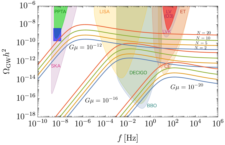
Figure 4: GW spectra from cosmic string loops calculated using extended VOS model for the case of $G\mu=10^{-12},10^{-16},10^{-20},$ with $N=2,5,10,20$. We use the relation $P=1/N^{2}$ for F-strings. Green and red shaded regions are excluded by PPTA [139] and aLIGO/aVirgo [140], respectively. Dense blue region highlights the potential signals by NANOGrav [141] and PPTA [142]. The lightly shaded regions represent the future sensitivities of GW experiments.

We numerically solve the extended VOS equation and calculate the GW spectrum without assuming scaling solution. The result is shown in Fig. 4 for the case of $G\mu=10^{-12}$, $10^{-16}$, and $10^{-20}$ with $N=2,5,10$, and $20$. We assume F-strings with $P=1/N^{2}$. We consider $\alpha=0.1$ and $N_{\rm scat}=10$. In particular, the case with $N=2$ corresponds to $P_{\rm eff}\simeq 0.94$, which is very close to unity. This reproduces the standard result for the case of $P_{\rm eff}=1$ within an $\mathcal{O}(1)$ factor. The resulting spectrum is in good agreement with the one shown in, e.g., Ref. [132].

The power-law-integrated sensitivity curves for ongoing and planned GW experiments are plotted according to Ref. [143], including SKA [47], LISA [48], DECIGO [144, 145], BBO [146], Einstein Telescope (ET) [147, 148], Cosmic Explorer (CE) [149], and aLIGO+aVirgo+KAGRA (LVK) [150, 151]. The current constraint from Parkes Pulsar Timing Array (PPTA) [139] and aLIGO/aVirgo’s third observing run (LV(O3)) [140] are indicated by the dense green and red shaded regions, respectively. The blue box near the bottom of the PPTA constraint highlights the potential signals of pulsar timing array (PTA) experiments, such as NANOGrav [141] and PPTA [142].

The GW spectrum shows a peak at a certain frequency, and below this frequency, it scales as $\Omega_{\rm GW}\propto f^{3/2}$. The amplitude of GW and frequency at the peak are approximately given by

$$\left(\Omega_{\rm GW}h^{2}\right)^{(\rm peak)}\simeq 2.5\times 10^{-10}\times P_{\rm eff}^{-1}\left(\frac{G\mu}{10^{-12}}\right)^{1/2},$$ (5.27)

$$f^{(\rm peak)}\simeq 1.9\times 10^{-6}\,{\rm Hz}\times\left(\frac{G\mu}{10^{-12}}\right)^{-1}.$$ (5.28)

It is observed that the dependence on $N$ and $\Lambda$ (or $P_{\rm eff}$ and $G\mu$) is not degenerate around the peak, and thus, we can determine both if we can observe the spectrum around the peak. Fortunately, this is within the sensitivity curve for the GW experiments, such as LISA, for the most parameter region of interest. We have also shown that the result of Eq. (5.20) agrees with our numerical results within a limit of large $f$.

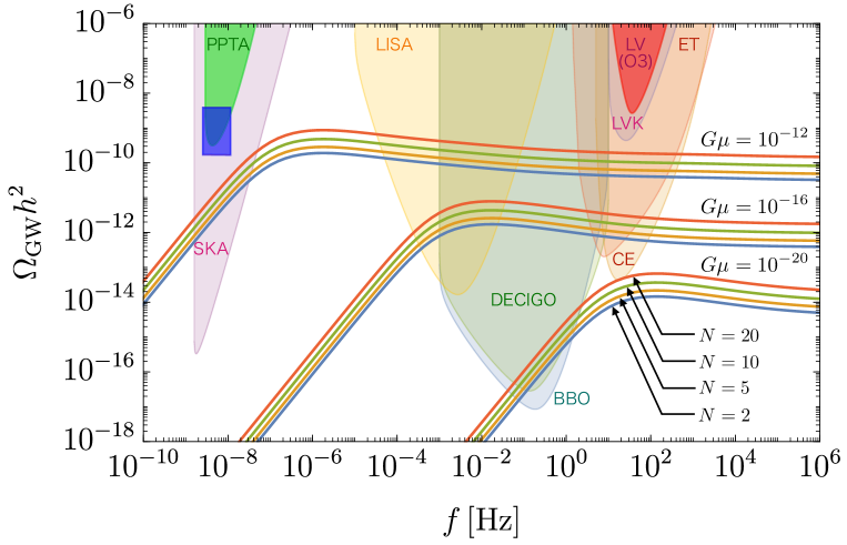
Figure 5: Same as Fig. 4 but with the standard VOS model ($\xi=L$) and the replacement of $\tilde{c}\to\tilde{c}P_{\rm eff}^{\gamma}$ with $\gamma=1/3$ and with $\alpha=0.3P_{\rm eff}^{\gamma}$.

To compare the standard result for a small intercommutation probability, we also solve the standard VOS model (that is, $\xi=L$) by replacing $\tilde{c}\to\tilde{c}P_{\rm eff}^{\gamma}$ with $\gamma=1/3$ and with $\alpha=0.3P_{\rm eff}^{\gamma}$ [132]. The resulting GW spectrum is shown in Fig. 5 for the same parameters with Fig. 4. The effect of small intercommutation probability is milder than the case with the extended VOS model because in this case, $(\Omega_{\rm gw}h^{2})^{\rm(scaling)}\propto P_{\rm eff}^{-2\gamma}\alpha^{1/2}\propto P_{\rm eff}^{-1/2}$ in the scaling regime.

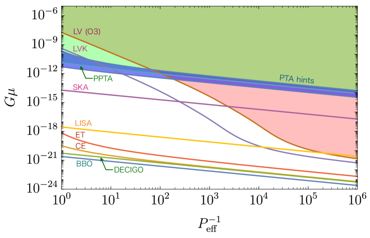
Figure 6: Exclusion plot and future sensitivity curves in $G\mu$ - $P_{\rm eff}^{-1}$ plane for ongoing and planned GW experiments. Green and red shaded regions are excluded by PPTA [139] and aLIGO/aVirgo [140], respectively. Dense blue region highlights the potential signals by NANOGrav [141] and PPTA [142].

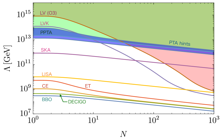
Figure 7: Same as Fig. 6 but in $\Lambda$ - $N$ plane for F-strings, wherein we treat $N$ as a continuous variable via the relation of $P_{\rm eff}=1-(1-P)^{N_{\rm scat}}$ with $P=1/N^{2}$ and $N_{\rm scat}=10$, although it must be an integer in a realistic model.

We show the constraints and sensitivity curves in terms of $G\mu$ and $P_{\rm eff}^{-1}$ in Fig. 6 using the extended VOS model. Each curve represents the lower bound on the parameter space wherein the predicted $\Omega_{\rm GW}h^{2}$ is greater than the sensitivity curve at a specific frequency. The green and red shaded regions are excluded by PPTA [139] and aLIGO/aVirgo [140], respectively. The dense blue region highlights the potential signals by NANOGrav [141] and PPTA [142]. The constraint on the string tension can be considerably strong for a large $P_{\rm eff}^{-1}$ by the ground-based GW experiments, such as aLIGO, aVirgo, and KAGRA. These experiments can search for GW signals from the scaling regime in the RD, wherein the spectrum scales as $\Omega_{\rm GW}h^{2}\propto\sqrt{G\mu}/P_{\rm eff}$ (see Eq. (5.20)). On the contrary, the sensitivity curves do not depend significantly on $P_{\rm eff}^{-1}$ for other experiments. This is because the peak frequency of the GW spectrum is too high to be detected by the latter experiments at a small $G\mu$, and in such cases, the GW signals decrease as $\Omega_{\rm GW}h^{2}\propto(G\mu)^{2}/P_{\rm eff}$ for $f\ll f^{\rm(peak)}$. If we consider $P_{\rm eff}\lesssim 0.1$, we can expect signals for aLIGO, aVirgo, and KAGRA consistently with the constraint from the PPTA. This is a unique feature of our model; the amplitude of GW can be enhanced by $P_{\rm eff}^{-1}$ without shifting its peak frequency.

We rewrite the sensitivities for $G\mu$ and $P_{\rm eff}^{-1}$ in terms of $\Lambda$ and $N$ by using the relations Eqs. (4.2), (4.4), and (4.5) for F-strings. Here we take $P=1/N^{2}$ though it has an $\mathcal{O}(1)$ uncertainty. The resulting sensitivity curves are shown in Fig. 7. Here, we treat $N$ as a continuous variable for the purpose of representation, although it must be an integer. We find that the present constraint puts an upper bound on the confinement scale as $\Lambda\lesssim 2\times 10^{13}\ {\rm GeV}$ for $N=\mathcal{O}(1)$. The NANOGrav and PPTA hints favor the parameter near the threshold of this constraint. There have been several studies on the GW signals from cosmic strings in this context [152, 153, 154]. We find that our cosmic strings could also explain the PTA hints when $G\mu\sim 10^{-10\,\text{-}\,12}$ or $\Lambda\sim 10^{13\,\text{-}\,14}\ {\rm GeV}$ for $N=\mathcal{O}(1)$. Here, it should be noted that

$$G\mu\simeq 2.8\times 10^{-14}\left(\frac{\Lambda}{10^{12}\ {\rm GeV}}\right)^{2},$$ (5.29)

where we use the lattice result of $\mu\simeq 4\Lambda^{2}$ for $\mathrm{SU}(N)$ [73].

The ongoing and planned GW experiments can search for the signals up to $\Lambda\gtrsim\mathcal{O}(10^{8})\ {\rm GeV}$. A large parameter space, spanning over five orders of magnitude, can be searched through the GW experiments. It can be inferred that such an intermediate scale for $\Lambda$ is naturally realized mainly because of the dimensional transmutation in the pure YM theory.

Finally, we discuss the constraint on cosmic strings from the CMB temperature and polarization data. The energy density of cosmic strings should be lower than the order 1% for the total temperature anisotoropy. From the detailed numerical simulations, the Planck result puts an upper bound on the string tension as $G\mu<1.1\times 10^{-7}$ for the ordinary Nambu-Goto cosmic strings [155]. The constraint should be stronger for strings with a small intercommutation probability because the energy density is $\rho_{\infty}\propto P_{\rm eff}^{-1}$. However, even if we include this enhancement factor, the constraint from CMB observations is much weaker than the present constraint evaluated through the GW experiments.

6 Discussion and conclusions

We have discussed that cosmic strings or macroscopic color flux tubes form at the deconfinement/confinement phase transition in pure YM theory. Depending on the structure of gauge group, these strings can be understood as fundamental (F-) strings and wrapped D-brane (which are referred to as D-strings) in the holographic dual descriptions, and possess a small intercommutation probability of $1/N^{2}$ and $e^{-\mathcal{O}(N)}$, respectively. We have explained that the cosmic strings have discrete 1-form symmetry, which further ensures stability. The 1-form symmetry also implies that $N$ cosmic strings can intersect at a baryon vertex for the case of $\mathrm{SU}(N)$. The network of the cosmic strings thus possess rich properties in the pure YM theory even if we do not assume brane inflationary scenario or extra dimensions. We have further discussed the types of cosmic strings formed in $\mathrm{SU}(N)$, $\mathrm{Sp}(N)$, $\mathrm{SO}(N)$, and $\mathrm{Spin}(N)$ YM theory, and we have explained the implications from electric–magnetic duality, large $N$ limit, as well as holographic dual descriptions.

We have considered an extended VOS model to take into account the small intercommutation probability and calculate the GW spectrum emitted from cosmic string loops. The GW signals can be observed through ongoing and planned GW experiments. Particularly, the SKA and LISA can observe GW signals if the confinement scale $\Lambda$ is higher than $\mathcal{O}(10^{12})\ {\rm GeV}$ and $\mathcal{O}(10^{10})\ {\rm GeV}$ for $N=\mathcal{O}(1)$, respectively. The DECIGO, BBO, CE, and ET could observe GW signals for $\Lambda\gtrsim\mathcal{O}(10^{8})\ {\rm GeV}$. The recently reported NANOGrav and PPTA hints favor $\Lambda=\mathcal{O}(10^{13})\ {\rm GeV}$.

Some assumptions should be confirmed through numerical simulations. The effect of small intercommutation probability is based on a numerical simulation of Ref. [46]. Although a common procedure used in the literature is the replacement of $\tilde{c}\to\tilde{c}P_{\rm eff}^{\gamma}$ with $\gamma=1/3$, the extended VOS model used in this paper and the aforementioned paper fits in well with the numerical result, and it seems to be physically reasonable. These procedures cannot be distinguished by the numerical results of the aforementioned paper, and thus, a numerical calculation with a larger simulation box is necessary. Moreover, as far as we know, there is no simulation for the network with baryon (or monopole) vertices that connect more than three cosmic strings. The formation of baryon vertices at the phase transition should also be confirmed through numerical simulations if the theories with the baryon vertices, such as $\mathrm{SU}(N)$, are considered. We expect that those properties can be understood by field-theory numerical simulations for a model of ${\mathbb{Z}}_{N}$ strings, where $\mathrm{SU}(N)$ symmetry is spontaneously broken to ${\mathbb{Z}}_{N}$ symmetry by $N$ adjoint Higgs fields. Another field-theory model is given in Eq. (3.1) based on the electric–magnetic duality.

These properties, namely the small intercommutation probability and existence of baryon vertices, are also realized by F-strings that form after the D-brane inflation. In the brane inflationary scenarios, bulk modes like radions and dilatons play essential roles and the extra dimensions are necessary. Our work provides another motivation to study the consequence of cosmic strings with the small intercommutation probability in a much simpler but phenomenologically and cosmologically interesting setup. Particularly, we do not need to consider extra dimensions for the UV completion. Moreover, the intercommutation probability is determined by $N$ in our case, and it is observed that the string tension is naturally small and does not require fine tuning by the dimensional transmutation. The GW signals are within the scope of future GW observations, such as SKA and LISA. Once the GW spectrum is observed, we can determine the confinement scale $\Lambda$ as well as $N$ for the pure YM theory.

We consider the case wherein the deconfinement/confinement phase transition occurs after inflation. Through lattice simulations of the $\mathrm{SU}(N)$ pure YM theory, the confinement phase transition is a second-order phase transition for $N=2$ and a first-order transition for $N\geq 3$ [156, 157, 158, 159, 160]. The GWs can also be produced from the collision of nucleated bubbled at the phase transition (see, e.g., Ref. [24]). This is another source of GW signals in the pure YM theory. However, the typical frequency is too high to be detected by GW experiments when the confinement scale is higher than $\mathcal{O}(10^{8})\ {\rm GeV}$. Thus, we can neglect it in our parameters of interest. The glueballs are also produced at the phase transition. Because the glueballs are singlet in the low-energy effective field theory, they should decay into other particles via higher-dimensional operators. In the presence of a light modulus, the glueball decay rate is estimated as $\Lambda^{6}/(4\pi m_{g}M^{4})$, where $m_{g}$ ($\sim\Lambda$) is the glueball mass and $M$ is a cutoff scale [22]. Because we focus on the case with $\Lambda\gtrsim 10^{8}\ {\rm GeV}$, the glueballs are expected to completely decay before the BBN epoch for $M=10^{16}\ {\rm GeV}$. The decay into axions is also efficient if the axion decay constant is small and/or the glueball mass is large. A recent work [23] discussed that the glueball can be long-lived in a model of “thermal squeezeout" and it dilutes cosmological relics, such as dark matter, by its late-time decay. The early matter-dominated epoch by the glueball domination may modify the GW spectrum at a high frequency even for a large dynamical scale.

Finally, we comment on the reheating after inflation. The phase transition need not necessarily occur after the reheating completes. The GWs for most frequencies of interest are emitted mainly from the string loops that are generated after the electroweak phase transition. The number density of string loops are determined using the scaling solution, which lose information related to the phase transition. Thus, our results can be applied for the cases wherein the cosmic strings reaches the scaling solution well before the electroweak phase transition. In particular, the phase transition can happen before the reheating is completed; for instance during the inflation-oscillation dominated era. Our scenario can be applied to the case where the maximal temperature of the Universe (which is usually much higher than the reheating temperature) and/or the Hubble parameter during inflation is higher than the confinement scale $\Lambda$. It is also observed that the scaling solution of cosmic strings is determined using the Hubble parameter, and it is independent of the temperature of the gauge sector (such as glueballs). Thus, our results do not change even if the temperature of the gauge sector is different from that of the SM sector.

References

- [1] L. B. Okun, THETONS, Pisma Zh. Eksp. Teor. Fiz. 31 (1979) 156.
- [2] L. B. Okun, THETA PARTICLES, Nucl. Phys. B 173 (1980) 1.
- [3] M. J. Strassler and K. M. Zurek, Echoes of a hidden valley at hadron colliders, Phys. Lett. B 651 (2007) 374 [hep-ph/0604261].
- [4] J. Kang and M. A. Luty, Macroscopic Strings and ’Quirks’ at Colliders, JHEP 11 (2009) 065 [0805.4642].
- [5] C. J. Morningstar and M. J. Peardon, The Glueball spectrum from an anisotropic lattice study, Phys. Rev. D 60 (1999) 034509 [hep-lat/9901004].
- [6] B. Lucini, A. Rago and E. Rinaldi, Glueball masses in the large N limit, JHEP 08 (2010) 119 [1007.3879].
- [7] D. Curtin, C. Gemmell and C. B. Verhaaren, Simulating Glueball Production in QCD, 2202.12899.
- [8] A. E. Faraggi and M. Pospelov, Selfinteracting dark matter from the hidden heterotic string sector, Astropart. Phys. 16 (2002) 451 [hep-ph/0008223].
- [9] J. L. Feng and Y. Shadmi, WIMPless Dark Matter from Non-Abelian Hidden Sectors with Anomaly-Mediated Supersymmetry Breaking, Phys. Rev. D 83 (2011) 095011 [1102.0282].
- [10] K. K. Boddy, J. L. Feng, M. Kaplinghat and T. M. P. Tait, Self-Interacting Dark Matter from a Non-Abelian Hidden Sector, Phys. Rev. D 89 (2014) 115017 [1402.3629].
- [11] K. K. Boddy, J. L. Feng, M. Kaplinghat, Y. Shadmi and T. M. P. Tait, Strongly interacting dark matter: Self-interactions and keV lines, Phys. Rev. D 90 (2014) 095016 [1408.6532].
- [12] A. Soni and Y. Zhang, Hidden SU(N) Glueball Dark Matter, Phys. Rev. D 93 (2016) 115025 [1602.00714].
- [13] G. D. Kribs and E. T. Neil, Review of strongly-coupled composite dark matter models and lattice simulations, Int. J. Mod. Phys. A 31 (2016) 1643004 [1604.04627].
- [14] L. Forestell, D. E. Morrissey and K. Sigurdson, Non-Abelian Dark Forces and the Relic Densities of Dark Glueballs, Phys. Rev. D 95 (2017) 015032 [1605.08048].
- [15] A. Soni, H. Xiao and Y. Zhang, Cosmic selection rule for the glueball dark matter relic density, Phys. Rev. D 96 (2017) 083514 [1704.02347].
- [16] L. Forestell, D. E. Morrissey and K. Sigurdson, Cosmological Bounds on Non-Abelian Dark Forces, Phys. Rev. D 97 (2018) 075029 [1710.06447].
- [17] B. Jo, H. Kim, H. D. Kim and C. S. Shin, Exploring the Universe with dark light scalars, Phys. Rev. D 103 (2021) 083528 [2010.10880].
- [18] D. N. Spergel and P. J. Steinhardt, Observational evidence for selfinteracting cold dark matter, Phys. Rev. Lett. 84 (2000) 3760 [astro-ph/9909386].
- [19] D. H. Weinberg, J. S. Bullock, F. Governato, R. Kuzio de Naray and A. H. G. Peter, Cold dark matter: controversies on small scales, Proc. Nat. Acad. Sci. 112 (2015) 12249 [1306.0913].
- [20] J. E. Juknevich, D. Melnikov and M. J. Strassler, A Pure-Glue Hidden Valley I. States and Decays, JHEP 07 (2009) 055 [0903.0883].
- [21] J. E. Juknevich, Pure-glue hidden valleys through the Higgs portal, JHEP 08 (2010) 121 [0911.5616].
- [22] J. Halverson, B. D. Nelson and F. Ruehle, String Theory and the Dark Glueball Problem, Phys. Rev. D 95 (2017) 043527 [1609.02151].
- [23] P. Asadi, E. D. Kramer, E. Kuflik, T. R. Slatyer and J. Smirnov, Glueballs in a Thermal Squeezeout Model, 2203.15813.
- [24] M. Reichert, F. Sannino, Z.-W. Wang and C. Zhang, Dark confinement and chiral phase transitions: gravitational waves vs matter representations, JHEP 01 (2022) 003 [2109.11552].
- [25] D. Gaiotto, A. Kapustin, N. Seiberg and B. Willett, Generalized Global Symmetries, JHEP 02 (2015) 172 [1412.5148].
- [26] G. ’t Hooft, On the Phase Transition Towards Permanent Quark Confinement, Nucl. Phys. B 138 (1978) 1.
- [27] G. ’t Hooft, A Property of Electric and Magnetic Flux in Nonabelian Gauge Theories, Nucl. Phys. B 153 (1979) 141.
- [28] E. Witten, Cosmic Superstrings, Phys. Lett. B 153 (1985) 243.
- [29] T. Vachaspati and A. Vilenkin, Evolution of cosmic networks, Phys. Rev. D 35 (1987) 1131.
- [30] N. Seiberg and E. Witten, Electric - magnetic duality, monopole condensation, and confinement in N=2 supersymmetric Yang-Mills theory, Nucl. Phys. B 426 (1994) 19 [hep-th/9407087].
- [31] G. ’t Hooft, A Planar Diagram Theory for Strong Interactions, Nucl. Phys. B 72 (1974) 461.
- [32] S. Coleman, Aspects of Symmetry: Selected Erice Lectures. Cambridge University Press, Cambridge, U.K., 1985, 10.1017/CBO9780511565045.
- [33] E. Witten, Anti-de Sitter space, thermal phase transition, and confinement in gauge theories, Adv. Theor. Math. Phys. 2 (1998) 505 [hep-th/9803131].
- [34] J. Polchinski and M. J. Strassler, The String dual of a confining four-dimensional gauge theory, hep-th/0003136.
- [35] I. R. Klebanov and M. J. Strassler, Supergravity and a confining gauge theory: Duality cascades and chi SB resolution of naked singularities, JHEP 08 (2000) 052 [hep-th/0007191].
- [36] J. M. Maldacena and C. Nunez, Towards the large N limit of pure N=1 superYang-Mills, Phys. Rev. Lett. 86 (2001) 588 [hep-th/0008001].
- [37] C. Vafa, Superstrings and topological strings at large N, J. Math. Phys. 42 (2001) 2798 [hep-th/0008142].
- [38] G. Dvali and A. Vilenkin, Formation and evolution of cosmic D strings, JCAP 03 (2004) 010 [hep-th/0312007].
- [39] E. J. Copeland, R. C. Myers and J. Polchinski, Cosmic F and D strings, JHEP 06 (2004) 013 [hep-th/0312067].
- [40] A. Vilenkin, Gravitational radiation from cosmic strings, Phys. Lett. B 107 (1981) 47.
- [41] T. Vachaspati and A. Vilenkin, Gravitational Radiation from Cosmic Strings, Phys. Rev. D 31 (1985) 3052.
- [42] T. W. B. Kibble, Evolution of a system of cosmic strings, Nucl. Phys. B 252 (1985) 227.
- [43] C. J. A. P. Martins and E. P. S. Shellard, String evolution with friction, Phys. Rev. D 53 (1996) 575 [hep-ph/9507335].
- [44] C. J. A. P. Martins and E. P. S. Shellard, Quantitative string evolution, Phys. Rev. D 54 (1996) 2535 [hep-ph/9602271].
- [45] C. J. A. P. Martins and E. P. S. Shellard, Extending the velocity dependent one scale string evolution model, Phys. Rev. D 65 (2002) 043514 [hep-ph/0003298].
- [46] A. Avgoustidis and E. P. S. Shellard, Effect of reconnection probability on cosmic (super)string network density, Phys. Rev. D 73 (2006) 041301 [astro-ph/0512582].
- [47] G. Janssen et al., Gravitational wave astronomy with the SKA, PoS AASKA14 (2015) 037 [1501.00127].
- [48] LISA collaboration, P. Amaro-Seoane et al., Laser Interferometer Space Antenna, 1702.00786.
- [49] Y. Hidaka, M. Nitta and R. Yokokura, Emergent discrete 3-form symmetry and domain walls, Phys. Lett. B 803 (2020) 135290 [1912.02782].
- [50] Y. Hidaka, Y. Hirono and R. Yokokura, Counting Nambu-Goldstone Modes of Higher-Form Global Symmetries, Phys. Rev. Lett. 126 (2021) 071601 [2007.15901].
- [51] Y. Hidaka, M. Nitta and R. Yokokura, Higher-form symmetries and 3-group in axion electrodynamics, Phys. Lett. B 808 (2020) 135672 [2006.12532].
- [52] Y. Hidaka, M. Nitta and R. Yokokura, Global 3-group symmetry and ’t Hooft anomalies in axion electrodynamics, JHEP 01 (2021) 173 [2009.14368].
- [53] Y. Hidaka, M. Nitta and R. Yokokura, Topological axion electrodynamics and 4-group symmetry, Phys. Lett. B 823 (2021) 136762 [2107.08753].
- [54] Y. Hidaka, M. Nitta and R. Yokokura, Global 4-group symmetry and ’t Hooft anomalies in topological axion electrodynamics, 2108.12564.
- [55] M. Nitta, Relations among topological solitons, 2202.03929.
- [56] C. Cordova, K. Ohmori and T. Rudelius, Generalized Symmetry Breaking Scales and Weak Gravity Conjectures, 2202.05866.
- [57] N. Yamamoto and R. Yokokura, Unstable Nambu-Goldstone modes, 2203.02727.
- [58] E. Witten, Supersymmetric index of three-dimensional gauge theory, hep-th/9903005.
- [59] E. Witten, Supersymmetric index in four-dimensional gauge theories, Adv. Theor. Math. Phys. 5 (2002) 841 [hep-th/0006010].
- [60] E. Poppitz, Notes on Confinement on R3 × S1: From Yang–Mills, Super-Yang–Mills, and QCD (adj) to QCD(F), Symmetry 14 (2022) 180 [2111.10423].
- [61] A. Vilenkin, COSMOLOGICAL EVOLUTION OF MONOPOLES CONNECTED BY STRINGS, Nucl. Phys. B 196 (1982) 240.
- [62] R. Donagi and E. Witten, Supersymmetric Yang-Mills theory and integrable systems, Nucl. Phys. B 460 (1996) 299 [hep-th/9510101].
- [63] M. G. Jackson, N. T. Jones and J. Polchinski, Collisions of cosmic F and D-strings, JHEP 10 (2005) 013 [hep-th/0405229].
- [64] M. R. Douglas and S. H. Shenker, Dynamics of SU(N) supersymmetric gauge theory, Nucl. Phys. B 447 (1995) 271 [hep-th/9503163].
- [65] A. Hanany, M. J. Strassler and A. Zaffaroni, Confinement and strings in MQCD, Nucl. Phys. B 513 (1998) 87 [hep-th/9707244].
- [66] C. P. Herzog and I. R. Klebanov, On string tensions in supersymmetric SU(M) gauge theory, Phys. Lett. B 526 (2002) 388 [hep-th/0111078].
- [67] H. Firouzjahi, L. Leblond and S. H. Henry Tye, The (p,q) string tension in a warped deformed conifold, JHEP 05 (2006) 047 [hep-th/0603161].
- [68] S. B. Giddings, S. Kachru and J. Polchinski, Hierarchies from fluxes in string compactifications, Phys. Rev. D 66 (2002) 106006 [hep-th/0105097].
- [69] O. Aharony, A Note on the holographic interpretation of string theory backgrounds with varying flux, JHEP 03 (2001) 012 [hep-th/0101013].
- [70] S. S. Gubser, C. P. Herzog and I. R. Klebanov, Symmetry breaking and axionic strings in the warped deformed conifold, JHEP 09 (2004) 036 [hep-th/0405282].
- [71] E. Witten, Baryons and branes in anti-de Sitter space, JHEP 07 (1998) 006 [hep-th/9805112].
- [72] E. Witten, Baryons in the 1/n Expansion, Nucl. Phys. B 160 (1979) 57.
- [73] A. Athenodorou and M. Teper, SU(N) gauge theories in 3+1 dimensions: glueball spectrum, string tensions and topology, JHEP 12 (2021) 082 [2106.00364].
- [74] J. Polchinski, Collision of Macroscopic Fundamental Strings, Phys. Lett. B 209 (1988) 252.
- [75] A. Hanany and K. Hashimoto, Reconnection of colliding cosmic strings, JHEP 06 (2005) 021 [hep-th/0501031].
- [76] C. J. A. P. Martins and E. P. S. Shellard, Fractal properties and small-scale structure of cosmic string networks, Phys. Rev. D 73 (2006) 043515 [astro-ph/0511792].
- [77] N. T. Jones, H. Stoica and S. H. H. Tye, Brane interaction as the origin of inflation, JHEP 07 (2002) 051 [hep-th/0203163].
- [78] S. Sarangi and S. H. H. Tye, Cosmic string production towards the end of brane inflation, Phys. Lett. B 536 (2002) 185 [hep-th/0204074].
- [79] G. Dvali and A. Vilenkin, Solitonic D-branes and brane annihilation, Phys. Rev. D 67 (2003) 046002 [hep-th/0209217].
- [80] N. T. Jones, H. Stoica and S. H. H. Tye, The Production, spectrum and evolution of cosmic strings in brane inflation, Phys. Lett. B 563 (2003) 6 [hep-th/0303269].
- [81] L. Pogosian, S. H. H. Tye, I. Wasserman and M. Wyman, Observational constraints on cosmic string production during brane inflation, Phys. Rev. D 68 (2003) 023506 [hep-th/0304188].
- [82] E. J. Copeland, T. W. B. Kibble and D. A. Steer, Collisions of strings with Y junctions, Phys. Rev. Lett. 97 (2006) 021602 [hep-th/0601153].
- [83] E. J. Copeland, T. W. B. Kibble and D. A. Steer, Constraints on string networks with junctions, Phys. Rev. D 75 (2007) 065024 [hep-th/0611243].
- [84] E. J. Copeland, H. Firouzjahi, T. W. B. Kibble and D. A. Steer, On the Collision of Cosmic Superstrings, Phys. Rev. D 77 (2008) 063521 [0712.0808].
- [85] A. Avgoustidis and E. P. S. Shellard, Velocity-Dependent Models for Non-Abelian/Entangled String Networks, Phys. Rev. D 78 (2008) 103510 [0705.3395].
- [86] A. Rajantie, M. Sakellariadou and H. Stoica, Numerical experiments with p F- and q D-strings: The Formation of (p,q) bound states, JCAP 11 (2007) 021 [0706.3662].
- [87] A. Pourtsidou, A. Avgoustidis, E. J. Copeland, L. Pogosian and D. A. Steer, Scaling configurations of cosmic superstring networks and their cosmological implications, Phys. Rev. D 83 (2011) 063525 [1012.5014].
- [88] L. Sousa and P. P. Avelino, Probing Cosmic Superstrings with Gravitational Waves, Phys. Rev. D 94 (2016) 063529 [1606.05585].
- [89] Y. Ng, T. W. B. Kibble and T. Vachaspati, Formation of Non-Abelian Monopoles Connected by Strings, Phys. Rev. D 78 (2008) 046001 [0806.0155].
- [90] D. Spergel and U.-L. Pen, Cosmology in a string dominated universe, Astrophys. J. Lett. 491 (1997) L67 [astro-ph/9611198].
- [91] P. McGraw, Evolution of a nonAbelian cosmic string network, Phys. Rev. D 57 (1998) 3317 [astro-ph/9706182].
- [92] M. Hindmarsh and T. W. B. Kibble, BEADS ON STRINGS, Phys. Rev. Lett. 55 (1985) 2398.
- [93] V. Berezinsky and A. Vilenkin, Cosmic necklaces and ultrahigh-energy cosmic rays, Phys. Rev. Lett. 79 (1997) 5202 [astro-ph/9704257].
- [94] M. Hindmarsh, K. Rummukainen and D. J. Weir, Numerical simulations of necklaces in SU(2) gauge-Higgs field theory, Phys. Rev. D 95 (2017) 063520 [1611.08456].
- [95] M. Yamada and K. Yonekura, In preparation, .
- [96] X. Artru, String Model with Baryons: Topology, Classical Motion, Nucl. Phys. B 85 (1975) 442.
- [97] E. J. Copeland and P. M. Saffin, On the evolution of cosmic-superstring networks, JHEP 11 (2005) 023 [hep-th/0505110].
- [98] M. Hindmarsh and P. M. Saffin, Scaling in a SU(2) model of cosmic superstring networks, JHEP 08 (2006) 066 [hep-th/0605014].
- [99] J. Urrestilla and A. Vilenkin, Evolution of cosmic superstring networks: A Numerical simulation, JHEP 02 (2008) 037 [0712.1146].
- [100] D. N. Spergel, N. Turok, W. H. Press and B. S. Ryden, Global texture as the origin of large scale structure: numerical simulations of evolution, Phys. Rev. D 43 (1991) 1038.
- [101] T. Hiramatsu, M. Kawasaki and K. Saikawa, Evolution of String-Wall Networks and Axionic Domain Wall Problem, JCAP 08 (2011) 030 [1012.4558].
- [102] T. Hiramatsu, M. Kawasaki, K. Saikawa and T. Sekiguchi, Axion cosmology with long-lived domain walls, JCAP 01 (2013) 001 [1207.3166].
- [103] M. Kawasaki, K. Saikawa and T. Sekiguchi, Axion dark matter from topological defects, Phys. Rev. D 91 (2015) 065014 [1412.0789].
- [104] T. Banks and N. Seiberg, Symmetries and Strings in Field Theory and Gravity, Phys. Rev. D 83 (2011) 084019 [1011.5120].
- [105] M. Montero, A. M. Uranga and I. Valenzuela, A Chern-Simons Pandemic, JHEP 07 (2017) 123 [1702.06147].
- [106] D. Harlow and H. Ooguri, Symmetries in quantum field theory and quantum gravity, Commun. Math. Phys. 383 (2021) 1669 [1810.05338].
- [107] T. Rudelius and S.-H. Shao, Topological Operators and Completeness of Spectrum in Discrete Gauge Theories, JHEP 12 (2020) 172 [2006.10052].
- [108] K. Yonekura, Topological violation of global symmetries in quantum gravity, JHEP 09 (2021) 036 [2011.11868].
- [109] B. Heidenreich, J. McNamara, M. Montero, M. Reece, T. Rudelius and I. Valenzuela, Chern-Weil global symmetries and how quantum gravity avoids them, JHEP 11 (2021) 053 [2012.00009].
- [110] B. Heidenreich, J. McNamara, M. Montero, M. Reece, T. Rudelius and I. Valenzuela, Non-invertible global symmetries and completeness of the spectrum, JHEP 09 (2021) 203 [2104.07036].
- [111] W. Buchmuller, V. Domcke and K. Schmitz, Stochastic gravitational-wave background from metastable cosmic strings, JCAP 12 (2021) 006 [2107.04578].
- [112] D. I. Dunsky, A. Ghoshal, H. Murayama, Y. Sakakihara and G. White, Gravitational Wave Gastronomy, 2111.08750.
- [113] G. Lazarides, R. Maji and Q. Shafi, Gravitational Waves from Quasi-stable Strings, 2203.11204.
- [114] M. A. Luty and T. Okui, Conformal technicolor, JHEP 09 (2006) 070 [hep-ph/0409274].
- [115] M. Ibe, Y. Nakayama and T. T. Yanagida, Conformal Gauge Mediation, Phys. Lett. B 649 (2007) 292 [hep-ph/0703110].
- [116] T. T. Yanagida and K. Yonekura, A Conformal Gauge Mediation and Dark Matter with Only One Parameter, Phys. Lett. B 693 (2010) 281 [1006.2271].
- [117] K. Hamaguchi, K. Nakayama and N. Yokozaki, A Solution to the mu/Bmu Problem in Gauge Mediation with Hidden Gauge Symmetry, JHEP 08 (2012) 006 [1111.1601].
- [118] C. Ringeval, M. Sakellariadou and F. Bouchet, Cosmological evolution of cosmic string loops, JCAP 02 (2007) 023 [astro-ph/0511646].
- [119] J. J. Blanco-Pillado, K. D. Olum and B. Shlaer, Large parallel cosmic string simulations: New results on loop production, Phys. Rev. D 83 (2011) 083514 [1101.5173].
- [120] J. J. Blanco-Pillado, K. D. Olum and B. Shlaer, The number of cosmic string loops, Phys. Rev. D 89 (2014) 023512 [1309.6637].
- [121] J. J. Blanco-Pillado and K. D. Olum, Stochastic gravitational wave background from smoothed cosmic string loops, Phys. Rev. D 96 (2017) 104046 [1709.02693].
- [122] J. J. Blanco-Pillado, K. D. Olum and X. Siemens, New limits on cosmic strings from gravitational wave observation, Phys. Lett. B 778 (2018) 392 [1709.02434].
- [123] R. R. Caldwell and B. Allen, Cosmological constraints on cosmic string gravitational radiation, Phys. Rev. D 45 (1992) 3447.
- [124] M. R. DePies and C. J. Hogan, Stochastic Gravitational Wave Background from Light Cosmic Strings, Phys. Rev. D 75 (2007) 125006 [astro-ph/0702335].
- [125] S. A. Sanidas, R. A. Battye and B. W. Stappers, Constraints on cosmic string tension imposed by the limit on the stochastic gravitational wave background from the European Pulsar Timing Array, Phys. Rev. D 85 (2012) 122003 [1201.2419].
- [126] L. Sousa and P. P. Avelino, Stochastic Gravitational Wave Background generated by Cosmic String Networks: Velocity-Dependent One-Scale model versus Scale-Invariant Evolution, Phys. Rev. D 88 (2013) 023516 [1304.2445].
- [127] C. J. A. P. Martins, J. N. Moore and E. P. S. Shellard, A Unified model for vortex string network evolution, Phys. Rev. Lett. 92 (2004) 251601 [hep-ph/0310255].
- [128] D. P. Bennett and F. R. Bouchet, High resolution simulations of cosmic string evolution. 1. Network evolution, Phys. Rev. D 41 (1990) 2408.
- [129] B. Allen and E. P. S. Shellard, Cosmic string evolution: a numerical simulation, Phys. Rev. Lett. 64 (1990) 119.
- [130] M. Sakellariadou, A Note on the evolution of cosmic string/superstring networks, JCAP 04 (2005) 003 [hep-th/0410234].
- [131] M. Sakellariadou and A. Vilenkin, Cosmic-string evolution in flat space-time, Phys. Rev. D 42 (1990) 349.
- [132] P. Auclair et al., Probing the gravitational wave background from cosmic strings with LISA, JCAP 04 (2020) 034 [1909.00819].
- [133] C. J. Burden, Gravitational Radiation From a Particular Class of Cosmic Strings, Phys. Lett. B 164 (1985) 277.
- [134] D. Garfinkle and T. Vachaspati, Radiation From Kinky, Cuspless Cosmic Loops, Phys. Rev. D 36 (1987) 2229.
- [135] A. Vilenkin and E. P. S. Shellard, Cosmic Strings and Other Topological Defects. Cambridge University Press, 7, 2000.
- [136] Planck collaboration, N. Aghanim et al., Planck 2018 results. VI. Cosmological parameters, Astron. Astrophys. 641 (2020) A6 [1807.06209].
- [137] R. A. Battye, R. R. Caldwell and E. P. S. Shellard, Gravitational waves from cosmic strings, in Conference on Topological Defects and CMB, pp. 11–31, 6, 1997, astro-ph/9706013.
- [138] Y. Cui, M. Lewicki, D. E. Morrissey and J. D. Wells, Probing the pre-BBN universe with gravitational waves from cosmic strings, JHEP 01 (2019) 081 [1808.08968].
- [139] R. M. Shannon et al., Gravitational waves from binary supermassive black holes missing in pulsar observations, Science 349 (2015) 1522 [1509.07320].
- [140] KAGRA, Virgo, LIGO Scientific collaboration, R. Abbott et al., Upper limits on the isotropic gravitational-wave background from Advanced LIGO and Advanced Virgo’s third observing run, Phys. Rev. D 104 (2021) 022004 [2101.12130].
- [141] NANOGrav collaboration, Z. Arzoumanian et al., The NANOGrav 12.5 yr Data Set: Search for an Isotropic Stochastic Gravitational-wave Background, Astrophys. J. Lett. 905 (2020) L34 [2009.04496].
- [142] B. Goncharov et al., On the Evidence for a Common-spectrum Process in the Search for the Nanohertz Gravitational-wave Background with the Parkes Pulsar Timing Array, Astrophys. J. Lett. 917 (2021) L19 [2107.12112].
- [143] K. Schmitz, New Sensitivity Curves for Gravitational-Wave Signals from Cosmological Phase Transitions, JHEP 01 (2021) 097 [2002.04615].
- [144] S. Kawamura et al., The Japanese space gravitational wave antenna: DECIGO, Class. Quant. Grav. 28 (2011) 094011.
- [145] S. Kawamura et al., Current status of space gravitational wave antenna DECIGO and B-DECIGO, PTEP 2021 (2021) 05A105 [2006.13545].
- [146] G. M. Harry, P. Fritschel, D. A. Shaddock, W. Folkner and E. S. Phinney, Laser interferometry for the big bang observer, Class. Quant. Grav. 23 (2006) 4887.
- [147] M. Punturo et al., The Einstein Telescope: A third-generation gravitational wave observatory, Class. Quant. Grav. 27 (2010) 194002.
- [148] M. Maggiore et al., Science Case for the Einstein Telescope, JCAP 03 (2020) 050 [1912.02622].
- [149] D. Reitze et al., Cosmic Explorer: The U.S. Contribution to Gravitational-Wave Astronomy beyond LIGO, Bull. Am. Astron. Soc. 51 (2019) 035 [1907.04833].
- [150] KAGRA collaboration, K. Somiya, Detector configuration of KAGRA: The Japanese cryogenic gravitational-wave detector, Class. Quant. Grav. 29 (2012) 124007 [1111.7185].
- [151] KAGRA collaboration, T. Akutsu et al., Overview of KAGRA : KAGRA science, 2008.02921.
- [152] J. Ellis and M. Lewicki, Cosmic String Interpretation of NANOGrav Pulsar Timing Data, Phys. Rev. Lett. 126 (2021) 041304 [2009.06555].
- [153] S. Blasi, V. Brdar and K. Schmitz, Has NANOGrav found first evidence for cosmic strings?, Phys. Rev. Lett. 126 (2021) 041305 [2009.06607].
- [154] J. J. Blanco-Pillado, K. D. Olum and J. M. Wachter, Comparison of cosmic string and superstring models to NANOGrav 12.5-year results, Phys. Rev. D 103 (2021) 103512 [2102.08194].
- [155] T. Charnock, A. Avgoustidis, E. J. Copeland and A. Moss, CMB constraints on cosmic strings and superstrings, Phys. Rev. D 93 (2016) 123503 [1603.01275].
- [156] Y. Iwasaki, K. Kanaya, T. Yoshie, T. Hoshino, T. Shirakawa, Y. Oyanagi et al., Finite temperature phase transition of SU(3) gauge theory on N(t) = 4 and 6 lattices, Phys. Rev. D 46 (1992) 4657.
- [157] G. Boyd, J. Engels, F. Karsch, E. Laermann, C. Legeland, M. Lutgemeier et al., Thermodynamics of SU(3) lattice gauge theory, Nucl. Phys. B 469 (1996) 419 [hep-lat/9602007].
- [158] B. Lucini, M. Teper and U. Wenger, The High temperature phase transition in SU(N) gauge theories, JHEP 01 (2004) 061 [hep-lat/0307017].
- [159] S. Datta and S. Gupta, Scaling and the continuum limit of the finite temperature deconfinement transition in SU pure gauge theory, Phys. Rev. D 80 (2009) 114504 [0909.5591].
- [160] M. Panero, Thermodynamics of the QCD plasma and the large-N limit, Phys. Rev. Lett. 103 (2009) 232001 [0907.3719].
- [161] O. Aharony, J. Sonnenschein and S. Yankielowicz, A Holographic model of deconfinement and chiral symmetry restoration, Annals Phys. 322 (2007) 1420 [hep-th/0604161].
- [162] G. Mandal and T. Morita, Gregory-Laflamme as the confinement/deconfinement transition in holographic QCD, JHEP 09 (2011) 073 [1107.4048].
- [163] H. Isono, G. Mandal and T. Morita, Thermodynamics of QCD from Sakai-Sugimoto Model, JHEP 12 (2015) 006 [1507.08949].
- [164] D. Gaiotto, A. Kapustin, Z. Komargodski and N. Seiberg, Theta, Time Reversal, and Temperature, JHEP 05 (2017) 091 [1703.00501].
- [165] Z. Komargodski, T. Sulejmanpasic and M. Ünsal, Walls, anomalies, and deconfinement in quantum antiferromagnets, Phys. Rev. B 97 (2018) 054418 [1706.05731].
- [166] H. Shimizu and K. Yonekura, Anomaly constraints on deconfinement and chiral phase transition, Phys. Rev. D 97 (2018) 105011 [1706.06104].
- [167] Y. Tanizaki, T. Misumi and N. Sakai, Circle compactification and ’t Hooft anomaly, JHEP 12 (2017) 056 [1710.08923].
- [168] Y. Tanizaki, Y. Kikuchi, T. Misumi and N. Sakai, Anomaly matching for the phase diagram of massless -QCD, Phys. Rev. D 97 (2018) 054012 [1711.10487].
- [169] K. Yonekura, Anomaly matching in QCD thermal phase transition, JHEP 05 (2019) 062 [1901.08188].