Estimation of Recursive Route Choice Models with Incomplete Trip Observations

Abstract

This work concerns the estimation of recursive route choice models in the situation that the trip observations are incomplete, i.e., there are unconnected links (or nodes) in the observations. A direct approach to handle this issue would be intractable because enumerating all paths between unconnected links (or nodes) in a real network is typically not possible. We exploit an expectation-maximization (EM) method that allows to deal with the missing-data issue by alternatively performing two steps of sampling the missing segments in the observations and solving maximum likelihood estimation problems. Moreover, observing that the EM method would be expensive, we propose a new estimation method based on the idea that the choice probabilities of unconnected link observations can be exactly computed by solving systems of linear equations. We further design a new algorithm, called as decomposition-composition (DC), that helps reduce the number of systems of linear equations to be solved and speed up the estimation. We compare our proposed algorithms with some standard baselines using a dataset from a real network, and show that the DC algorithm outperforms the other approaches in recovering missing information in the observations. Our methods work with most of the recursive route choice models proposed in the literature, including the recursive logit, nested recursive logit, or discounted recursive models.

Keywords: Incomplete observation, recursive logit, nested recursive logit, expectation-maximization, decomposition-composition.

1 Introduction

Travel demand modeling plays a vital role in transportation planning, operations, and management. In travel demand modeling, route choice is a process that associates the behaviors of selecting a route to travel from an origin to a destination. Such a route choice model can be used to assess travelers’ preferences regarding characteristics of different routes and travellers (e.g. travel time, travel cost, number of crossings, or age, gender, and trip purpose of the travellers). Route choice models can also be used to predict traffic flows and can have applications in traffic simulation (Osorio and Chong, 2015) or network pricing (Zimmermann et al., 2021). The parameters of a route choice model are often estimated using path observations collected by, for instance, Global Positioning System (GPS) devices equipped on vehicles. It is commonly known that such trip observations would be incomplete due to several reasons, for example, the GPS signals are intermittent or some parts of the GPS data are censored from the analyst due to privacy concerns. This missing data issue is critical for the estimation of route choice models but to the best of our knowledge, this issue has not been properly investigated in the context of route choice modeling. We address the issue in this paper.

We focus on link-based recursive route choice models (Fosgerau et al., 2013, Mai et al., 2015) due to their several advantages, namely, the estimation does not require sampling of route choice alternatives and the models can be consistently estimated and easy to predict. Such a recursive model is based on the Rust’s dynamic discrete choice framework (Rust, 1987) where a path choice is modelled as a sequence of link choices and the parameters are estimated by combining maximum likelihood estimation (MLE) and dynamic programming (see Zimmermann and Frejinger, 2020, for a tutorial). A naive approach to deal with the missing-data issue under recursive models is to ignore the unconnected link observations and solve the MLE problem only based on connected ones. This approach can be done straightforwardly using existing estimation algorithms (Fosgerau et al., 2013, Mai et al., 2015, 2018). However, unconnected segments in the observations would contain valuable information about traveller route choice behavior and would be important for the estimation. In this paper, we aim at developing new estimation algorithms that allow us to efficiently and practically recover information from these incomplete segments.

Our contributions: We make a number of contributions in this work. We first exploit the expectation-maximization (EM) method to deal with the missing-data issue. This method has been widely used to estimate statistical models with unobserved variables (Dempster et al., 1977, McLachlan et al., 2019) and we show how this scheme can be used in the context of route choice modeling under recursive models. More precisely, we design an EM algorithm that alternatively performs two steps where the first step is to compute an expected log-likelihood function by sampling paths to fill unconnected segments in the observations, and the second step maximizes that expected log-likelihood function. We further show that, under the recursive logit model (Fosgerau et al., 2013), the expected log-likelihood function is concave, thus the second step can be done efficiently by convex optimization.

Moreover, observing that the EM algorithm would be expensive to perform as it requires solving several MLE problems, we further propose a new method to directly compute the probabilities of unconnected path segments. That is, we show that the probability of unconnected links can be obtained by solving one system of linear equations. This result allows us to compute the likelihood function of the incomplete observations where the missing segments are explicitly taken into consideration. Furthermore, to reduce the number of systems of linear equations to be solved and speed up the estimation process, we develop a new algorithm, called as the decomposition-composition (DC) method. The idea is to decompose each linear system above into two parts and compose the common parts to reduce the number of linear systems to be solved. The main advantage of our DC algorithm is that we only need to solve only one system of linear equations to obtain all the choice probabilities of unconnected segments on trips that share the same destination. We also show that such a system of linear questions always has a unique solution.

We test our proposed algorithms with two popular recursive route choice models, i.e., the recursive logit (RL) (Fosgerau et al., 2013) and nested recursive logit (NRL) models, using a dataset collected from a real network. Our numerical experiments clearly show that our DC algorithm outperforms the EM and other baseline approaches in recovering missing information from observations. Our numerical results are based on the RL and NRL models, but our method can be applied to other existing recursive models in the literature, e.g., the recursive network multivariate extreme value (Mai, 2016), discounted RL (Oyama and Hato, 2017), or stochastic time-dependent RL (Mai et al., 2021).

Literature reviews: The literature on route choice modeling covers path-based and link-based recursive models. Path-based models (see Prato, 2009, for a review) rely on sampling of paths, thus the parameter estimates would depend on the sampling methods. Even when corrections are added to the choice probabilities to achieve consistent estimates, the prediction is not easy to perform. In contrast, the link-based recursive models are built based on the dynamic discrete choice framework (Rust, 1987) and they are basically equivalent to discrete choice models based on the sets of all possible paths. Link-based recursive models have several advantages, making them attractive recently, for instance, the models can be consistently estimated and can be quickly and easily used for prediction. The first recursive model (i.e. the RL model) is proposed by Fosgerau et al. (2013). Several recursive models have been developed afterwards to deal with, for instance, correlations between path utilities (Mai et al., 2015, Mai, 2016, Mai et al., 2018), dynamic networks (de Moraes Ramos et al., 2020), stochastic time-dependent networks (Mai et al., 2021), or discounted behavior (Oyama and Hato, 2017), with applications in, for instance, traffic management (Baillon and Cominetti, 2008, Melo, 2012) or network pricing (Zimmermann et al., 2021). We refer the reader to Zimmermann and Frejinger (2020) for a comprehensive review.

With the development of technology and the ease of accessing the Internet, onboard devices, e.g., GPS, are more commonly used for several purposes, including rote navigation for taxis, buses, trucks, passenger cars, utility vehicles, mobile phones, etc. From operations and management perspectives, GPS data can be utilized to understand route choice behaviors. In fact, GPS has been used for collecting data for route choice modelling from a very early time (Wolf et al., 1999). Some other early studies used GPS data for modelling the route choice of vehicles (Gilani, 2005), cyclists and pedestrians (Krizek et al., 2007, Dill and Gliebe, 2008, Menghini et al., 2010, Broach et al., 2012), transit (Oliveira and Casas, 2010), and commuting (Papinski et al., 2009). While collecting data by GPS brings many advantages, it is frequent that GPS data is missing or incomplete, leading to difficulties for analysis (Wang et al., 2011, Shen and Stopher, 2014). Consequently, researchers have developed various approaches to overcome this issue. For example, Smith et al. (2003) introduce a preliminary analysis of techniques for imputing missing data. The results revealed that the statistical technique outperformed the heuristics technique in terms of accuracy and performance. Melville et al. (2004) used an ensemble method which is available under the DECORATE package and found DECORATE is more robust to missing data than the other two methods. Some researchers combined map-matching (Bierlaire and Frejinger, 2008) or questionnaire surveys (de Moraes Ramos, 2015) which provide ground truth and improve the quality of the GPS data. We refer the reader to Shen and Stopher (2014) for a review of GPS travel surveys, applications, and data processing. In the context of route choice modeling, to deal with the missing-data issue, to the best of our knowledge, existing studies only focus on data collection, i.e., improving GPS data and the map-matching, and we seem to be the first to take the estimation of route choice models with missing data into consideration.

Our work also closely relates to the EM framework (Dempster et al., 1977, Gentle, 1998, Arcidiacono and Miller, 2011), which has been popularly used for estimating statistical models with latent variables or unknown data observations. It should be noted that an EM algorithm does increase the likelihood value of the observed data after each iteration, but there is no guarantee that the sequence converges to a maximum likelihood estimator (Gentle, 1998). In addition, the method requires repeatedly solving MLE problems, which would be expensive, especially in the context of recursive route choice models since the estimation of these models involves solving several dynamic programs (Mai and Frejinger, 2022).

Paper outline: This paper is organized as follows. Section 2 presents the recursive models and the missing-data issue. Section 3 presents our EM and Section 4 presents the DC algorithms. Section 5 reports numerical experiments, and finally, Section 6 concludes the study and provides directions for future research.

Notations: Boldface characters represent matrices (or vectors), and $a_{i}$ denotes the $i$-th element of vector a, $A_{i,j}$ denotes the $(i,j)$-th element of matrix A, and $\textbf{A}_{:,j}$ denotes the $j$-th column of matrix A. We use $[m]$, for any $m\in\mathbb{N}_{+}$, to denote the set $\{1,\ldots,m\}$.

2 Recursive Route Choice Models and the Missing Data Issue

Consider a network ${\mathcal{G}}=({\mathcal{A}},{\mathcal{V}})$, where ${\mathcal{A}}$ is the set of links and ${\mathcal{V}}$ is the set of nodes. Moreover, an absorbing state is associated with each destination by extending the network with dummy links $d$. The set of all links becomes $\widetilde{\mathcal{A}}=\mathcal{A}\cup\{d\}$. For each link $k\in{\mathcal{A}}$, let $A(k)$ be the set of outgoing links from $k$. For two links $k,a\in\widetilde{\mathcal{A}}$, the instantaneous utility $u(a|k)=v(a|k)+\epsilon(a|k)$, where $v(a|k)$ is the deterministic part of the utility and $\epsilon(a)$ is a random term with zero mean. We assume that $v(a|k)$, for all $a\in A(k)$ to be negative for all links except the dummy link $d$.

For any link $k\in\mathcal{A}$, let $V(k)$ be the expected maximum utility (i.e., the value function) from the sink node of $k$ to the destination. In a recursive route choice model (Fosgerau et al., 2013, Mai et al., 2015), a choice of route is modelled as a sequence of link choices, in which at each link, the traveller selects an outgoing link by maximizing the sum of link utility and the expected maximum utility from that link to the destination. The selection of the next link can be written as in the following form $a=\text{argmax}_{a^{\prime}\in A(k)}\left\{v(a^{\prime}|k)+V(a^{\prime})+\epsilon(a^{\prime}|k)\right\}$. The value function $V(k)$ thus can be computed recursively as

$$V(k)=\begin{cases}{\mathbb{E}}_{\epsilon}\left[\max_{a\in A(k)}\left(v(a|k)+V(a)+\epsilon(a|k)\right)\right]&\text{ if }k\in{\mathcal{A}}\backslash\{d\}\\ 1&\text{ if }k=d\end{cases}$$ (1)

Here, we note that the value function should depend on the destination $d$ but we omit the corresponding indices for notational simplicity. Different assumptions can be made for the random terms $\epsilon(a|k)$. If we assume that $\epsilon(a|k)$, $\forall a\in A(k)$, are i.i.d Extreme Value Type I with scale $\mu>0$ and independent of everything in the network, the recursive model becomes the recursive logit (RL) (Fosgerau et al., 2013) in which the value function can be computed conveniently as

$$V(k)=\begin{cases}\mu\ln\left(\sum_{a\in A(k)}\exp\left(\frac{1}{\mu}\left(v(a|k)+V(a)\right)\right)\right)&\forall k\in{\mathcal{A}}\backslash\{d\}\\ 1&\text{ if }k=d.\end{cases}$$ (2)

The above recursive formulation has an appealing property that it can be written as a system of linear equations. More precisely, if we define a vector Z of size $|\widetilde{\mathcal{A}}|$ with elements $Z_{k}=\exp(V(k)/\mu)$, for all $k\in\widetilde{\mathcal{A}}$, a matrix M of size $(|\widetilde{\mathcal{A}}|\times|\widetilde{\mathcal{A}}|)$ with elements $M_{ka}=\mathbb{I}(a\in A(k))\exp\left(v(a|k)/\mu\right)$, and b is a vector of size $|\widetilde{\mathcal{A}}|$ with zero elements everywhere except $b_{d}=1$, then (2) can be reformulated as a system of linear equations as $\textbf{Z}={\textbf{M}}\textbf{Z}+\textbf{b}$. Such a system can be solved quickly using an iterative algorithm implemented in some existing linear solvers (Mai et al., 2015, 2018).

It is well-known that the RL model retains the independence from irrelevance alternatives (IIA) property (Fosgerau et al., 2013, Mai et al., 2015), which would not hold in some real-life applications. To relax this property, Mai et al. (2015) propose the NRL model based on the assumption that the random terms $\epsilon(a|k)$ have different scale parameters over links, i.e., $\epsilon(a|k)=\mu_{k}\epsilon^{\prime}(a|k)$, $\forall k\in{\mathcal{A}}$, where $\epsilon^{\prime}(a|k)$ are i.i.d extreme value type I for all $k,a\in\widetilde{\mathcal{A}},a\in A(k)$. The value function in the NRL model can be defined recursively as

$$V(k)=\begin{cases}\mu_{k}\ln\left(\sum_{a\in A(k)}\exp\left(\frac{1}{\mu_{k}}\left(v(a|k)+V(a)\right)\right)\right)&\forall k\in{\mathcal{A}}\backslash\{d\}\\ 1&\text{ if }k=d.\end{cases}$$ (3)

Then, by defining matrix M of size $(|\widetilde{\mathcal{A}}|\times|\widetilde{\mathcal{A}}|)$ with entries $M_{ka}=\mathbb{I}(a\in A(k))\exp\left(v(a|k)/\mu_{k}\right)$, $\forall a,k\in\widetilde{\mathcal{A}}$, Z of size $|\widetilde{\mathcal{A}}|$ with entries $Z_{k}=\exp(v(k)/\mu_{k})$, the Bellman equation leads to the system of nonlinear equations $Z_{k}=\sum_{a\in A(k)}M_{ka}Z_{a}^{\phi_{ka}}+b_{k}$, $\forall k\in{\mathcal{A}}$. This system can be solved by a value iteration or least-squares approach (Mai and Frejinger, 2022).

Recursive route choice models aforementioned can be estimated via MLE, which requires to compute log-likelihood values of some path observations. Given a complete path $\sigma=\{k_{0},\ldots,k_{{\mathcal{T}}}=d\}$, the probability of choosing this path can be computed as

$$P(\sigma|{\boldsymbol{\theta}})=\prod_{t=0}^{{\mathcal{T}}-1}P(k_{t+1}|k_{t};{\boldsymbol{\theta}}),$$

where ${\boldsymbol{\theta}}$ is the model parameters to be estimated and $P(k_{t+1}|k_{t};{\boldsymbol{\theta}})$ is the probability of moving from link $k_{t}$ to $k_{t+1}$. The link choice probabilities $P(a|k)$, $\forall a\in A(k)$ can be further computed using the value function $V(k)$, $\forall k\in{\mathcal{A}}$. For instance, for the RL model, we can compute $P(a|k)$ as

$$P(a|k)=\exp\left(\frac{1}{\mu}\left(v(a|k)+V(a)-V(k)\right)\right),$$

and for the NRL, the link choice probabilities can be computed as

$$P(a|k)=\exp\left(\frac{1}{\mu_{k}}\left(v(a|k)+V(a)-V(k)\right)\right).$$

In the case that path observation $\sigma$ is not complete, i.e., there is at least one pair of successive link observations $(k_{t},k_{t+1})$ such that $k_{t+t}\notin A(k_{t})$, the computation of $P(\sigma)$ is much more challenging. To elaborate this point, let consider a link choice probability $P(a|k)$ where link $a$ is not connected to $k$, i.e., $a\notin A(k)$. Basically, $P(a|k)$ is referred to the probability of reaching link $a$ from $k$ conditional on the current parameters and the destination $d$. This probability can be written as

$$P(a|k)=\sum_{\sigma\in\Omega^{ka}}P(\sigma),$$ (4)

where $\Omega^{ka}$ is the set of all possible paths going from $k$ to $a$ and $P(\sigma)$ is the probability of (complete) path $\sigma$, which can be computed through link choice probabilities of connected links. Enumerating all paths from $k$ to $a$ is typically not feasible, in particular with real networks. So, a direct approach to deal with missing data is practical. In the next sections, we present our ways to address this issue, i.e., one is based on the EM scheme (Dempster et al., 1977), and the other one is a direct approach to compute the log-likelihood function of incomplete observations.

3 The Expectation-Maximization Algorithm

We explore the EM method (Dempster et al., 1977, Arcidiacono and Miller, 2011) to handle the data missing issue. Such an EM algorithm will alternate an expectation (E) step, which creates a function for the expectation of the log-likelihood (LL) evaluated using the current estimate for the parameters ${\boldsymbol{\theta}}$, and a maximization (M) step that maximizes the expectation function created by the E step. In the following, we show how this method can be applied to estimate recursive route choice models with incomplete observations.

We first denote by $\Phi=\{\sigma_{1},\ldots,\sigma_{N}\}$ the set of $N$ observed paths. This set may contain some incomplete paths. We further denote by ${\boldsymbol{\Gamma}}=\{\Gamma_{1},\ldots,\Gamma_{N}\}$ the random variables representing the hidden parts of the observations. Each $\Gamma_{n}$ corresponds to $\sigma_{n}$ such that if $\gamma_{n}$ is a realization of $\Gamma_{n}$, then $(\sigma_{n},\gamma_{n})$ forms a complete path. Given a realization ${\boldsymbol{\gamma}}=\{\gamma_{1},\ldots,\gamma_{N}\}$ of ${\boldsymbol{\Gamma}}$, we define $L({\boldsymbol{\theta}};\Phi,{\boldsymbol{\gamma}})$ be the LL function of the complete observations $\Phi\cup{\boldsymbol{\gamma}}$. To perform the two EM steps, we define $R({\boldsymbol{\theta}}|\bar{{\boldsymbol{\theta}}})$ as the expected value of the LL function of the observations w.r.t the current conditional distribution of ${\boldsymbol{\Gamma}}$ given the observed set $\Phi$ and the current estimate $\bar{{\boldsymbol{\theta}}}$ of the model parameters ${\boldsymbol{\theta}}$. The function $R({\boldsymbol{\theta}}|\bar{{\boldsymbol{\theta}}})$ has the following form

$$R({\boldsymbol{\theta}}|\bar{{\boldsymbol{\theta}}}) ={\mathbb{E}}_{{\boldsymbol{\Gamma}}|\Phi,\bar{{\boldsymbol{\theta}}}}\left[L({\boldsymbol{\theta}};\Phi,{\boldsymbol{\Gamma}})\right]$$ (5)

$$=\sum_{n\in[N]}{\mathbb{E}}_{\Gamma_{n}|\sigma_{n},\bar{{\boldsymbol{\theta}}}}\left[\ln P(\sigma_{n},\Gamma_{n}|{\boldsymbol{\theta}})\right].$$

Since $(\sigma_{n},\gamma_{n})$ forms a complete path for all $n\in[N]$, $P(\sigma_{n},\gamma_{n}|{\boldsymbol{\theta}})$ can be written as a product of choice probabilities of connected links. To compute the expectation in (5), we consider $\sigma_{n}$ as a set of pairs of links and we separate each $\sigma_{n}$ into two sets of pairs of links $\sigma^{1}_{n}$ and $\sigma^{2}_{n}$ such that $\sigma^{1}_{n}$ contains all the connected pairs of links, i.e., $\sigma^{1}_{n}=\{(g,h)\in\sigma_{n}|\ h\in A(g)\}$ and $\sigma^{2}_{n}=\sigma_{n}\backslash\sigma^{1}_{n}$. This allows us to write (5) as

$$R({\boldsymbol{\theta}}|\bar{{\boldsymbol{\theta}}}) =\sum_{n\in[N]}{\mathbb{E}}_{\Gamma_{n}|\sigma_{n},\bar{{\boldsymbol{\theta}}}}\left[\sum_{\varsigma\in\sigma^{1}_{n}}\ln P(\varsigma|{\boldsymbol{\theta}})+\sum_{\varsigma\in\Gamma_{n}}\ln P(\varsigma|{\boldsymbol{\theta}})\right]$$

$$=\sum_{n\in[N]}\sum_{\varsigma\in\sigma^{1}_{n}}\ln P(\varsigma|{\boldsymbol{\theta}})+\sum_{n\in[N]}{\mathbb{E}}_{\Gamma_{n}|\sigma_{n},\bar{{\boldsymbol{\theta}}}}\left[\sum_{\varsigma\in\sigma_{n}^{2}}\ln P(\varsigma|{\boldsymbol{\theta}})\right]$$

$$=\sum_{n\in[N]}\sum_{\varsigma\in\sigma^{1}_{n}}\ln P(\varsigma|{\boldsymbol{\theta}})+\sum_{n\in[N]}\sum_{\varsigma\in\sigma^{2}_{n}}{\mathbb{E}}_{\Gamma^{n,\varsigma}|\;\bar{{\boldsymbol{\theta}}}}\big{[}\ln P(\Gamma^{n,\varsigma}|{\boldsymbol{\theta}})\big{]},$$ (6)

where $\Gamma^{n,\varsigma}$ is a random variable representing a complete path connecting the pair of unconnected pair $\varsigma\in\sigma^{2}_{n}$, ${\mathbb{E}}_{\Gamma^{n,\varsigma}|\varsigma,\bar{{\boldsymbol{\theta}}}}\big{[}\ln P(\Gamma^{n,\varsigma}|{\boldsymbol{\theta}})\big{]}$ is an expectation over $\Gamma^{n,\varsigma}$, and $P(\Gamma^{n,\varsigma}|{\boldsymbol{\theta}})$ is the probability of complete path $\Gamma^{n,\varsigma}$. Since $\Gamma^{n,\varsigma}$ is complete, $P(\Gamma^{n,\varsigma}|{\boldsymbol{\theta}})$ can be written as the product of choice probabilities of connected links.

An EM algorithm will perform alternatively E and M steps until converging to a fixed-point solution. At an E step and under a current estimate ${\boldsymbol{\theta}}^{t}$, we need to create function $R({\boldsymbol{\theta}}|{\boldsymbol{\theta}}^{t})$ based on $\Phi$ and the current parameters ${\boldsymbol{\theta}}^{t}$. Even though there may be infinite numbers of complete paths $\Gamma$ connecting a pair of links $\varsigma\in\sigma^{2}_{n}$, we can approximate the expectation by sampling as

$$\hat{R}({\boldsymbol{\theta}}|{\boldsymbol{\theta}}^{t})=\sum_{n\in[N]}\sum_{\varsigma\in\sigma^{1}_{n}}\ln P(\varsigma|{\boldsymbol{\theta}})+\sum_{n\in[N]}\sum_{\varsigma\in\sigma^{2}_{n}}\sum_{s\in[S]}\ln P(\gamma^{n,\varsigma}_{s}|{\boldsymbol{\theta}})P(\gamma^{n,\varsigma}_{s}|\varsigma,{\boldsymbol{\theta}}^{t})/{\mathcal{P}}^{n,\varsigma}({\boldsymbol{\theta}}^{t}),$$ (7)

where $\gamma^{n,\varsigma}_{1},\ldots,\gamma^{n,\varsigma}_{S}$ are $S$ realizations of $\Gamma^{n,\varsigma}$, $P(\gamma^{n,\varsigma}_{s}|\varsigma,{\boldsymbol{\theta}}^{t})$ is the probability of the path $\gamma^{n,\varsigma}_{s}$ given a pair of links $\varsigma$ and conditional on the current estimate ${\boldsymbol{\theta}}^{t}$, and ${\mathcal{P}}^{n,\varsigma}({\boldsymbol{\theta}}^{t})=\sum_{s\in[S]}P(\gamma^{n,\varsigma}_{s}|\varsigma,{\boldsymbol{\theta}}^{t})$. Here, for ease of notation, we assume that the numbers of samples $S$ are the same over $\varsigma$. If it is not the case, we always can generate some dummy paths with zero probabilities. Typically, when the sample size $S$ is large enough, the left-hand side of (7) will converge to the true $R({\boldsymbol{\theta}}|{\boldsymbol{\theta}}^{t})$ with probability one due to the law of large number.

To sample from the conditional distribution of $\Gamma^{n,\varsigma}$ given a pair $\varsigma=(k,a)$, $a\notin A(k)$, and parameters ${\boldsymbol{\theta}}^{t}$, we can generate paths that connect these two links according to the link probabilities $P(h|g;{\boldsymbol{\theta}}^{t})$, $\forall h\in A(g)$. The probability $P(\gamma^{n,\varsigma}|\;{\boldsymbol{\theta}}^{t})$ can be computed by multiplying the link choice probabilities $P(h|g;{\boldsymbol{\theta}}^{t})$ for every connected pair $(g,h)$ on $\gamma^{n,\varsigma}$. In summary, we describe the EM algorithm in Algorithm 1 below.

Choose a converge threshold $\xi>0$, set $t=0$, choose an initial parameter vector ${\boldsymbol{\theta}}^{0}$.

do

      

• E step: For each observation $\sigma_{n}$ and for each unconnected pair $\varsigma\in\sigma^{2}_{n}$, generate paths $\gamma^{n,\varsigma}_{1},\ldots,\gamma^{n,\varsigma}_{S}$ connecting that pair according to the link choice probabilities $P(h|g;{\boldsymbol{\theta}}^{t})$, $\forall h\in A(g)$. Compute $P(\gamma^{n,\varsigma}_{s}|{\boldsymbol{\theta}}^{t})$, $s\in[S]$. Create function $\hat{R}({\boldsymbol{\theta}}|{\boldsymbol{\theta}}^{t})$ using (7).

• M step: Choose next ${\boldsymbol{\theta}}^{t+1}$ by maximizing $\widehat{R}({\boldsymbol{\theta}}|{\boldsymbol{\theta}}^{t})$

  $${\boldsymbol{\theta}}^{t+1}=\text{argmax}_{{\boldsymbol{\theta}}}\widehat{R}({\boldsymbol{\theta}}|{\boldsymbol{\theta}}^{t}).$$ (8)

$t\leftarrow t+1$

while $||{\boldsymbol{\theta}}^{t}-{\boldsymbol{\theta}}^{t+1}||\geq\xi$ /* not converged to a stationary point */

Algorithm 1 EM algorithm

The EM algorithm iterative performs the E and M steps and stops when it converges to a fixed point solution, i.e., ${\boldsymbol{\theta}}^{t}$ is sufficiently closed to ${\boldsymbol{\theta}}^{t+1}$. It generates a sequence $\{{\boldsymbol{\theta}}^{1},{\boldsymbol{\theta}}^{2},\ldots\}$ such that the marginal likelihood of the data $L(\Phi|{\boldsymbol{\theta}})=\int L({\boldsymbol{\theta}};\Phi,\Gamma)d\Gamma$ is non-decreasing. In general, the algorithm does not guarantee that the sequence $\{{\boldsymbol{\theta}}^{t}\}$ converges to a maximum likelihood estimator, but typically, the derivative of the likelihood function will be arbitrarily close to zero at the fixed point (Dempster et al., 1977, Arcidiacono and Miller, 2011).

The M step of the EM algorithm involves solving a continuous maximization problem $\max_{{\boldsymbol{\theta}}}\hat{R}({\boldsymbol{\theta}}|{\boldsymbol{\theta}}^{t})$. The computation of $\hat{R}({\boldsymbol{\theta}}|{\boldsymbol{\theta}}^{t})$ and its gradient w.r.t. ${\boldsymbol{\theta}}$ can be done by computing the value function $V$ and its Jacobian. As mentioned earlier, these value functions can be obtained via solving systems of linear equations for the RL model, and via value iteration for the NRL model. In the context of RL, it can be shown that $\widehat{R}({\boldsymbol{\theta}}|{\boldsymbol{\theta}}^{t})$ can be written as a sum of the logarithm of the choice probabilities of several complete paths. As a result, if the link utilities $v(a|k)$, $\forall a,k\in\widetilde{\mathcal{A}}$ are linear in ${\boldsymbol{\theta}}$, then $\widehat{R}({\boldsymbol{\theta}}|{\boldsymbol{\theta}}^{t})$ is concave in ${\boldsymbol{\theta}}$, making the maximization problem in Algorithm 1 tractable, noting that this linear-in-parameters setting is common in most of the existing route choice modeling studies (Prato, 2012, Fosgerau et al., 2013, Mai et al., 2015). We state this result in the following proposition.

Proposition 1

Under the RL model, if the deterministic link utilities $v(a|k)$, $k,a\in\widetilde{\mathcal{A}}$, $a\in A(k)$, are linear in parameters ${\boldsymbol{\theta}}$, then $\widehat{R}({\boldsymbol{\theta}}|{\boldsymbol{\theta}}^{t})$ is concave in ${\boldsymbol{\theta}}$.

Proof. For notational simplicity, let us define $p^{n,\varsigma}_{s}=P(\gamma^{n,\varsigma}_{s}|\varsigma,{\boldsymbol{\theta}}^{t})/{\mathcal{P}}^{n,\varsigma}({\boldsymbol{\theta}}^{t})$, for all $n\in[N]$, $s\in[S]$, and $\varsigma\in\sigma^{2}_{n}$. For any $n,\varsigma$ we have $\sum_{s\in[S]}p^{n,\varsigma}_{s}=1$. We now assume that each $\sigma^{2}_{n}$ contains $K_{n}$ disconnected pairs, denoted as $\varsigma^{n}_{1},\ldots,\varsigma^{n}_{K_{n}}$ and let

$${\mathcal{S}}^{n}=\underbrace{[S]\times\ldots\times[S]}_{K_{n}\text{ times}},$$

recalling that $[S]=\{1,2,\ldots,S\}$. We now write $\widehat{R}({\boldsymbol{\theta}}|{\boldsymbol{\theta}}^{t})$ as

$$\widehat{R}({\boldsymbol{\theta}}|{\boldsymbol{\theta}}^{t}) =\sum_{n\in[N]}\sum_{\varsigma\in\sigma^{1}_{n}}\ln P(\varsigma|{\boldsymbol{\theta}})+\sum_{n\in[N]}\sum_{\varsigma\in\sigma^{2}_{n}}\sum_{s\in[S]}\ln P(\gamma^{n,\varsigma}_{s}|{\boldsymbol{\theta}})p^{n,\varsigma}_{s}$$ (9)

We now see that, for any $\varsigma^{n}_{i}\in\sigma^{2}_{n}$, $i\in[K_{n}]$, and $s\in[S]$, the term $\ln P(\gamma^{n,\varsigma^{n}_{i}}_{s}|{\boldsymbol{\theta}})p^{n,\varsigma^{n}_{i}}_{s}$ as

$$p^{n,\varsigma^{n}_{i}}_{s}\ln P(\gamma^{n,\varsigma^{n}_{i}}_{s}|{\boldsymbol{\theta}}) =\ln P(\gamma^{n,\varsigma^{n}_{i}}_{s}|{\boldsymbol{\theta}})\left(\prod_{\begin{subarray}{c}j\in[K_{n}]\\ j\neq i\end{subarray}}\left(\sum_{s^{\prime}\in[S]}p_{s^{\prime}}^{n,\varsigma^{n}_{j}}\right)\right)p^{n,\varsigma^{n}_{i}}_{s}$$

$$=\ln P(\gamma^{n,\varsigma^{n}_{i}}_{s}|{\boldsymbol{\theta}})\left(\sum_{\begin{subarray}{c}(s_{1},...,s_{K_{n}})\in{\mathcal{S}}^{n}\\ s_{i}=s\end{subarray}}\left(\prod_{j\in[K_{n}]}p^{n,\varsigma^{n}_{j}}_{s_{j}}\right)\right).$$ (10)

Moreover, we have

$$\sum_{\varsigma\in\sigma^{1}_{n}}\ln P(\varsigma|{\boldsymbol{\theta}})=\sum_{\varsigma\in\sigma^{1}_{n}}\ln P(\varsigma|{\boldsymbol{\theta}})\left(\sum_{\begin{subarray}{c}(s_{1},...,s_{K_{n}})\in{\mathcal{S}}^{n}\end{subarray}}\left(\prod_{j\in[K_{n}]}p^{n,\varsigma^{n}_{j}}_{s_{j}}\right)\right).$$ (11)

We now can combine (9)-(11) to have

$$\widehat{R}({\boldsymbol{\theta}}|{\boldsymbol{\theta}}^{t}) =\sum_{n\in[N]}\sum_{(s_{1},...,s_{K_{n}})\in{\mathcal{S}}^{n}}\left(\left(\prod_{i\in[K_{n}]}p^{n,\varsigma^{n}_{i}}_{s_{i}}\right)\left(\sum_{\varsigma\in\sigma^{1}_{n}}\ln P(\varsigma|{\boldsymbol{\theta}})+\sum_{i=1}^{K_{n}}\ln P(\gamma^{n,\varsigma^{n}_{i}}_{s_{i}}|{\boldsymbol{\theta}})\right)\right)$$

$$=\sum_{n\in[N]}\sum_{(s_{1},...,s_{K_{n}})\in{\mathcal{S}}^{n}}\left(\prod_{i\in[K_{n}]}p^{n,\varsigma^{n}_{i}}_{s_{i}}\right)\left(\ln P\left((\sigma_{n},\gamma^{n,\varsigma^{n}_{1}}_{s_{1}},...,\gamma^{n,\varsigma^{n}_{K_{n}}}_{s_{K_{n}}})|{\boldsymbol{\theta}}\right)\right),$$

where $P\left((\sigma_{n},\gamma^{n,\varsigma^{n}_{1}}_{s_{1}},...,\gamma^{n,\varsigma^{n}_{K_{n}}}_{s_{K_{n}}})|{\boldsymbol{\theta}}\right)$ is the probability of the (complete) path $(\sigma_{n},\gamma^{n,\varsigma^{n}_{1}}_{s_{1}},...,\gamma^{n,\varsigma^{n}_{K_{n}}}_{s_{K_{n}}})$. Fosgerau et al. (2013) show that the choice probability of a complete path can be written as

$$P\left((\sigma_{n},\gamma^{n,\varsigma^{n}_{1}}_{s_{1}},...,\gamma^{n,\varsigma^{n}_{K_{n}}}_{s_{K_{n}}})|{\boldsymbol{\theta}}\right)=\frac{\exp(v(\sigma_{n},\gamma^{n,\varsigma^{n}_{1}}_{s_{1}},...,\gamma^{n,\varsigma^{n}_{K_{n}}}_{s_{K_{n}}}|{\boldsymbol{\theta}}))}{\sum_{\tau\in\Omega^{n}}\exp(v(\tau|{\boldsymbol{\theta}}))},$$

where $v(\tau|{\boldsymbol{\theta}})$ is the deterministic utility of path $\tau$, i.e., $v(\tau)=\sum_{(k,a)\in\tau}v(a|k)$ and $\Omega^{n}$ is the set of all possible paths that share the same destination with observation $n$-th. Under the assumption that $v(a|k)$ is linear in ${\boldsymbol{\theta}}$, $v(\tau)$ is also linear in ${\boldsymbol{\theta}}$. As a result, we can write

$$\ln P\left((\sigma_{n},\gamma^{n,\varsigma^{n}_{1}}_{s_{1}},...,\gamma^{n,\varsigma^{n}_{K_{n}}}_{s_{K_{n}}})|{\boldsymbol{\theta}}\right)=v(\sigma_{n},\gamma^{n,\varsigma^{n}_{1}}_{s_{1}},...,\gamma^{n,\varsigma^{n}_{K_{n}}}_{s_{K_{n}}}|{\boldsymbol{\theta}})-\ln\left(\sum_{\tau\in\Omega^{n}}\exp v(\tau|{\boldsymbol{\theta}})\right)$$ (12)

The first term of (12) is linear in ${\boldsymbol{\theta}}$ and the second term has a log-sum-exp convex form of a geometric program, thus is convex in ${\boldsymbol{\theta}}$. So, $\ln P\left((\sigma_{n},\gamma^{n,\varsigma^{n}_{1}}_{s_{1}},...,\gamma^{n,\varsigma^{n}_{K_{n}}}_{s_{K_{n}}})|{\boldsymbol{\theta}}\right)$ is concave, thus $\widehat{R}({\boldsymbol{\theta}}|{\boldsymbol{\theta}}^{t})$ is concave, as desired.   

If the choice model is the NRL, the LL and $\widehat{R}({\boldsymbol{\theta}}|{\boldsymbol{\theta}}^{t})$ functions have highly nonlinear forms and are generally not concave. In this case, the M step of the EM algorithm may be difficult to handle globally. Moreover, it can be seen that the EM algorithm is generally expensive to perform, as it requires solving the maximization problem (8) several times until getting a fixed point solution. Furthermore, each maximization problem (8) requires sampling several paths between every unconnected pair of links to approximate the expectation ${R}({\boldsymbol{\theta}}|{\boldsymbol{\theta}}^{t})$, which is also expensive.

4 The Decomposition-Composition Algorithm

In this section, we propose a practical way to exactly compute the likelihood of incomplete observations. We then present our decomposition-composition method to speed up the computation of the LL function as well as its gradients.

4.1 Computing the Log-Likelihood of Incomplete Observations

Given an unconnected pair $(k,a)$ such that the link observations between these two links are missing. To compute the LL of the path that contain pair $(k,a)$, we need to compute $P(a|k)$, i.e., the probability of reaching $a$ from $k$. As mentioned earlier, this can be done by enumerating all possible paths between these two links, which would be not possible with a real network. To do this in a tractable way, we define $\pi^{a}(s)$ as the probability of reaching link $a\in\widetilde{\mathcal{A}}$ from link $s\in{\mathcal{A}}$. The values of $\pi^{a}(s)$, $\forall s,a\in\widetilde{\mathcal{A}}$, satisfies the following recursive equations

$$\pi^{a}(s)=\begin{cases}\sum_{s^{\prime}\in A(s)}P(s^{\prime}|s)\pi^{a}(s^{\prime})&\forall s\neq a\\ 1&s=a.\end{cases}$$ (13)

So, if we define $\textbf{h}^{a}$ as a vector of size $|\widetilde{\mathcal{A}}|$ with all zero elements except $h^{a}_{a}=1$ and a matrix $\textbf{Q}^{a}$ of size $(|\widetilde{\mathcal{A}}|\times|\widetilde{\mathcal{A}}|)$ with elements

$$\textbf{Q}^{a}_{s,s^{\prime}}=\begin{cases}P(s^{\prime}|s),&\forall s,s^{\prime}\in\widetilde{\mathcal{A}},\;s\neq a,s^{\prime}\in A(s)\\ 0&\text{ if }s=a,\end{cases}$$

then we can write (13) as

$$\boldsymbol{\pi}^{a}=\textbf{Q}^{a}\boldsymbol{\pi}^{a}+\textbf{h}^{a},\text{ or }\boldsymbol{\pi}^{a}=({\textbf{I}}-\textbf{Q}^{a})^{-1}\textbf{h}^{a},$$ (14)

where $\boldsymbol{\pi}^{a}$ is a vector of size $(|\widetilde{\mathcal{A}}|)$ with entries $\pi^{a}_{s}=\pi^{a}(s)$, $\forall s\in\widetilde{\mathcal{A}}$, and I is the identity matrix of size $(|\widetilde{\mathcal{A}}|\times|\widetilde{\mathcal{A}}|)$. Proposition 2 below shows that ${\textbf{I}}-\textbf{Q}^{a}$ is invertible, which guarantees the existence and uniqueness of the solutions to (14).

Proposition 2

For any $a\in\widetilde{\mathcal{A}}$, the matrix ${\textbf{I}}-\textbf{Q}^{a}$ is invertible.

Proof. For any $a\in\widetilde{\mathcal{A}}$, we have

$$\sum_{s^{\prime}\in\widetilde{\mathcal{A}}}\textbf{Q}^{a}_{s,s^{\prime}}=\begin{cases}\sum_{s^{\prime}\in\widetilde{\mathcal{A}}}P(s^{\prime}|s)=1&\text{ if }s\neq a\\ 0&\text{ if }s=a.\end{cases}$$

So, $\textbf{Q}^{a}$ is a sub-stochastic matrix (contains non-negative entries and every row adds up to at most 1). Moreover, $\textbf{Q}^{a}$ contains no recurrent class. So, $({\textbf{I}}-\textbf{Q}^{a})$ is invertible, as desired.   

So after computing $\boldsymbol{\pi}^{a}$, we can obtain $P(a|k)$ as $P(a|k)=\boldsymbol{\pi}^{a}_{k}$. We also need the gradients of $P(a|k)$ for the maximum likelihood estimation. Such gradient values can be obtained through taking the Jacobian of $\boldsymbol{\pi}^{a}$ w.r.t. parameter $\theta_{j}$ as

$$\frac{\partial\boldsymbol{\pi}^{a}}{\partial\theta_{j}}=-({\textbf{I}}-\textbf{Q}^{a})^{-1}\frac{\partial\textbf{Q}^{a}}{\partial\theta_{j}}({\textbf{I}}-\textbf{Q}^{a})^{-1}\textbf{h}^{a}=-({\textbf{I}}-\textbf{Q}^{a})^{-1}\frac{\partial\textbf{Q}^{a}}{\partial\theta_{j}}\boldsymbol{\pi}^{a},$$

where $\partial\textbf{Q}^{a}/\partial\theta_{j}$ is a matrix of size $|\widetilde{\mathcal{A}}|\times|\widetilde{\mathcal{A}}|$ with entries $\partial Q^{a}_{s,s^{\prime}}/\partial\theta_{j}$. This matrix can be obtained by taking gradients of $P(k^{\prime}|k)$ for all $k^{\prime},k\in\widetilde{\mathcal{A}},k^{\prime}\in A(k)$. These further can be computed by taking the gradients of the value functions, and the gradients of the value function $V(k)$ can be computed by solving some system of linear equations (Fosgerau et al., 2013, Mai et al., 2015). So, the Jacobian of $\boldsymbol{\pi}^{a}$ can be obtained by solving a series of systems of linear equations.

4.2 Decomposition-Composition Algorithm

In the above section, we show that the LL of incomplete observations can be computed directly by solving one system of linear equations for each unconnected pair $(k_{i},k_{i+1})$. This would be time-consuming if a path observation contains a large number of such unconnected pairs. We show in the following that it is possible to obtain the probabilities of all the unconnected pairs on paths that share the same destination by solving only one system of linear equations, instead of solving one linear system per each incomplete pair. The idea is to decompose each individual system of linear equations into two parts among which one part is the same over unconnected pairs. This allows us to compose all the individual linear systems into only one linear system.

For a path observation, assume that we observe $J$ incomplete pairs $\{(u_{1},v_{1})$,…, $(u_{J},v_{J})\}$, $(u_{j},v_{j})\in\widetilde{\mathcal{A}}\times\widetilde{\mathcal{A}}$, $\forall j=1,\ldots,J$. We define a matrix $\textbf{Q}^{0}$ of size $((|\widetilde{\mathcal{A}}|+1)\times(|\widetilde{\mathcal{A}}|+1)$ with entries

$$\textbf{Q}^{0}_{s,s^{\prime}} =P(s^{\prime}|s),\ \forall s,s^{\prime}\in\widetilde{\mathcal{A}},s^{\prime}\in A(s)$$

$$\textbf{Q}^{0}_{s,|\widetilde{\mathcal{A}}|+1} =\textbf{Q}^{0}_{|\widetilde{\mathcal{A}}|+1,s}=0,\ \forall s\in\mathcal{A}.$$

That is, the last row and last column of $\textbf{Q}^{0}$ are all-zero vectors. We also define a matrix H of size $(|\widetilde{\mathcal{A}}|+1)\times K$ with entries

$$H_{s,k}=\begin{cases}1&\text{ if }s=|\widetilde{\mathcal{A}}|+1\text{ or }s=u_{k}\\ 0&\text{ otherwise. }\end{cases}$$

The following theorem show that one can obtain all the probabilities $P(v_{j}|u_{j})$, $j=1,\ldots,J$ by solving only one system of linear equations. Let we first denote by $\widetilde{{\textbf{I}}}$ as an identity matrix of size $(|\widetilde{\mathcal{A}}|+1)\times(|\widetilde{\mathcal{A}}|+1)$.

Theorem 1

The matrix $\widetilde{{\textbf{I}}}-\textbf{Q}^{0}$ is always invertible. Moreover, if $\boldsymbol{\Pi}$ is the unique solution to the system of linear equations $\boldsymbol{\Pi}=(\widetilde{{\textbf{I}}}-\textbf{Q}^{0})^{-1}\textbf{H}$, then $P(v_{j}|u_{j})={\Pi}_{v_{j},j},\;\forall j\in[J].$

Proof. To prove the invertibility, Let $\widehat{\textbf{Q}}=({\textbf{Q}}^{0})^{\mbox{\tiny T}}$, we can see that $\widehat{Q}_{s,s^{\prime}}\geq 0$ for all $s,s^{\prime}\in\widetilde{\mathcal{A}}$ and $\sum_{s^{\prime}\in A(s)}\widehat{Q}_{s,s^{\prime}}=1,\;\forall s\in\widetilde{\mathcal{A}}$ and $\sum_{s^{\prime}\in A(s)}\widehat{Q}_{s,s^{\prime}}=0$ if $s=|\widetilde{\mathcal{A}}|+1$. Thus $\widehat{\textbf{Q}}$ is a sub-stochastic matrix. Moreover, $\widehat{\textbf{Q}}$ contains no recurrent class, thus $(\widetilde{{\textbf{I}}}-\widehat{\textbf{Q}})$ is invertible. Moreover $(\widetilde{{\textbf{I}}}-\widehat{\textbf{Q}})^{\mbox{\tiny T}}=(\widetilde{{\textbf{I}}}-{\textbf{Q}}^{0})$, thus $\widetilde{{\textbf{I}}}-\textbf{Q}^{0}$ is invertible, as desired.

For the second claim of the theorem, let us consider a pair of missing data $(u_{j},v_{j})$. We create an artificial link $r$ such that it is impossible to reach $r$ from any other link in $\widetilde{\mathcal{A}}$ and from $r$ we can only reach $u_{k}$ with probability 1. Let $\pi^{j}(s)$, for all $s\in\mathcal{A}$ be the probability of reaching $s$ from $u_{j}$, i.e., $P(s|u_{j})$. We see that $\pi^{j}(s)$, $s\in\mathcal{A}$, satisfy the following recursive equations.

$$\pi^{j}(s)=\begin{cases}\sum_{s^{\prime}\in{\mathcal{A}}}P(s|s^{\prime})\pi^{j}(s^{\prime})&\forall s\in\mathcal{A}\\ 1&s=r.\end{cases}$$ (15)

Now, we define a matrix $\textbf{Q}^{j}$ of size $(|\widetilde{\mathcal{A}}|+1)\times(|\widetilde{\mathcal{A}}|+1)$ with elements $\textbf{Q}^{j}_{s,s^{\prime}}=P(s|s^{\prime})$, $\forall s,s^{\prime}\in\widetilde{\mathcal{A}}\cup\{r\},s\in A(s^{\prime})$, and a vector q of size $|\widetilde{\mathcal{A}}|+1$ with all zero elements except $q_{r}=1$. We also number $r$ as $|\widetilde{\mathcal{A}}|+1$, so the last column and row of $\textbf{Q}^{j}$ and the last element of q correspond to link $r$. (15) can be written as

$$\boldsymbol{\pi}^{j}=\textbf{Q}^{j}\boldsymbol{\pi}^{j}+\textbf{q}.$$ (16)

Note that the last row of $\textbf{Q}^{j}$ is an all-zero vector as $r$ is not reachable by any other links, and the last column of $\textbf{Q}^{j}$ has all zero entries except the element that corresponds to link $u_{j}$. We decompose (16) as

$$\textbf{Q}^{j}\boldsymbol{\pi}^{j}+\textbf{q} =\begin{pmatrix}\textbf{Q}^{j}_{1,1}&\textbf{Q}^{j}_{1,2}&\cdots&\textbf{Q}^{j}_{1,|\widetilde{\mathcal{A}}|+1}\\ \textbf{Q}^{j}_{2,1}&\textbf{Q}^{j}_{2,2}&\cdots&\textbf{Q}^{j}_{2,|\widetilde{\mathcal{A}}|+1}\\ \vdots&\vdots&\ddots&\vdots\\ 0&0&\cdots&0\end{pmatrix}\begin{pmatrix}\pi^{j}_{1}\\ \pi^{j}_{2}\\ \vdots\\ \pi^{j}_{|\widetilde{\mathcal{A}}|+1}\end{pmatrix}+\textbf{q}$$

$$\stackrel{{\scriptstyle(a)}}{{=}}\begin{pmatrix}0&0&\cdots&\textbf{Q}^{j}_{1,|\widetilde{\mathcal{A}}|}&0\\ 0&0&\cdots&\textbf{Q}^{j}_{2,|\widetilde{\mathcal{A}}|}&0\\ \vdots&\vdots&\ddots&\vdots&\vdots\\ 0&0&\cdots&\textbf{Q}^{j}_{2,|\widetilde{\mathcal{A}}|}&0\end{pmatrix}\boldsymbol{\pi}^{j}+\begin{pmatrix}0&0&\cdots&\textbf{Q}^{j}_{1,|\widetilde{\mathcal{A}}|+1}\\ 0&0&\cdots&\textbf{Q}^{j}_{2,|\widetilde{\mathcal{A}}|+1}\\ \vdots&\vdots&\ddots&\vdots\\ 0&0&\cdots&0\end{pmatrix}\begin{pmatrix}\pi^{j}_{1}\\ \pi^{j}_{2}\\ \vdots\\ \pi^{j}_{|\widetilde{\mathcal{A}}|+1}\end{pmatrix}+\textbf{q}$$

$$=\textbf{Q}^{0}\boldsymbol{\pi}^{j}+\begin{pmatrix}0&0&\cdots&\textbf{Q}^{j}_{1,|\widetilde{\mathcal{A}}|+1}\\ 0&0&\cdots&\textbf{Q}^{j}_{2,|\widetilde{\mathcal{A}}|+1}\\ \vdots&\vdots&\ddots&\vdots\\ 0&0&\cdots&0\end{pmatrix}\begin{pmatrix}\pi^{j}_{1}\\ \pi^{j}_{2}\\ \vdots\\ \pi^{j}_{|\widetilde{\mathcal{A}}|+1}\end{pmatrix}+\textbf{q}$$

$$\stackrel{{\scriptstyle}}{{=}}\textbf{Q}^{0}\boldsymbol{\pi}^{j}+\begin{pmatrix}\textbf{Q}^{j}_{1,|\widetilde{\mathcal{A}}|+1}\\ \textbf{Q}^{j}_{2,|\widetilde{\mathcal{A}}|+1}\\ \vdots\\ 0\end{pmatrix}\pi^{j}_{|\widetilde{\mathcal{A}}|+1}+\textbf{q}$$

where for (a) we separate $\textbf{Q}^{j}$ into two parts; the first part contains all the columns of $\textbf{Q}^{j}$ except the last column and the second part only contains the last column of $\textbf{Q}^{j}$. We now note that the last column of $\textbf{Q}^{j}$ have zero element except the one corresponding to $u_{j}$. Moreover $\pi^{j}_{|\widetilde{\mathcal{A}}|+1}=1$, thus $(Q^{j}_{1,|\widetilde{\mathcal{A}}|+1},\ldots,Q^{j}_{|\widetilde{\mathcal{A}}|+1,|\widetilde{\mathcal{A}}|+1})^{\mbox{\tiny T}}\pi^{j}_{|\widetilde{\mathcal{A}}|+1}$ is a vector of zero elements except the one at $u_{k}$, which is equal to 1. Thus,

$$\begin{pmatrix}\textbf{Q}^{j}_{1,|\widetilde{\mathcal{A}}|+1}\\ \textbf{Q}^{j}_{2,|\widetilde{\mathcal{A}}|+1}\\ \vdots\\ 0\end{pmatrix}\pi^{j}_{|\widetilde{\mathcal{A}}|+1}+\textbf{q}$$

is also the $j$-th column of matrix H defined above. So, we have

$$\textbf{Q}^{j}\boldsymbol{\pi}^{j}+\textbf{q}=\textbf{Q}^{0}\boldsymbol{\pi}^{j}+\textbf{H}_{:,j},$$

where $\textbf{H}_{:,k}$ is the $j$-th column of H. So, $\boldsymbol{\pi}^{j}$ is a solution to the following system

$$(\widetilde{{\textbf{I}}}-\textbf{Q}^{0})\boldsymbol{\pi}^{j}=\textbf{D}_{:,j},$$

where $\widetilde{{\textbf{I}}}$ is an identity matrix of size $(|\widetilde{\mathcal{A}}|+1)\times(|\widetilde{\mathcal{A}}|+1)$. This also means that if matrix $\boldsymbol{\Pi}$ is a solution to the system of linear equations $(\widetilde{{\textbf{I}}}-\textbf{Q}^{0})\boldsymbol{\Pi}=\textbf{D}$ or $\boldsymbol{\Pi}=(\widetilde{{\textbf{I}}}-\textbf{Q}^{0})^{-1}\textbf{H}$, then

$$\boldsymbol{\pi}^{j}=\boldsymbol{\Pi}_{:,j}\text{ and }{\Pi}_{v_{j},j}=\boldsymbol{\pi}^{j}(v_{j})=P(v_{j}|u_{j}),$$

which is the desired result.   

For the MLE, the gradients of $P(v_{j}|u_{j})$ are required. The gradient of $P(v_{j}|u_{j})$ w.r.t. a parameter $\theta_{t}$ can also be obtained by computing the Jacobian of $\boldsymbol{\Pi}$, which can be obtained by solving the following linear system

$$\frac{\partial\boldsymbol{\Pi}}{\partial{\boldsymbol{\theta}}_{t}}=(\widetilde{{\textbf{I}}}-\textbf{Q}^{0})^{-1}\frac{\partial\textbf{Q}^{0}}{\partial{\boldsymbol{\theta}}_{t}}(\widetilde{{\textbf{I}}}-\textbf{Q}^{0})^{-1}\textbf{H}=(\widetilde{{\textbf{I}}}-\textbf{Q}^{0})^{-1}\frac{\partial\textbf{Q}^{0}}{\partial{\boldsymbol{\theta}}_{t}}\boldsymbol{\Pi}.$$ (17)

Since $\widetilde{{\textbf{I}}}-\textbf{Q}^{0}$ is invertible, the linear system in (17) always has a unique solution.

Algorithm 2 below describes the basic steps of our Decomposition-Composition (DC) algorithm (the term “Decomposition-Composition” refers to the fact that we decompose matrix $\textbf{Q}^{j}$ into two parts where one of them is the same over unconnected pairs $(u_{j},v_{j})$, and then compose all the individual linear systems into only one system of linear equations).

/* Run a nonlinear optimization algorithm (gradient accent or trust region or linear search (Nocedal and Wright, 2006a)) to estimate the model parameters ${\boldsymbol{\theta}}$. */

while not converged do

      

• Compute the value function Z as well as its gradients by value iteration and/or solving systems of linear equations, as shown in Fosgerau et al. (2013), Mai et al. (2015)

• Compute link choice probabilities $P(a|k)$, for all $k,a\in\widetilde{\mathcal{A}},a\in A(k)$ and their gradients

• Solve the linear system $\boldsymbol{\Pi}=(\widetilde{{\textbf{I}}}-\textbf{Q}^{0})^{-1}\textbf{H}$ and (17) to get the probabilities of unconnected pairs $(u_{j},v_{j})$, $j=1,\ldots,J$, as well as their gradients.

• Compute the log-likelihood of the (incomplete) observations and its gradient w.r.t. ${\boldsymbol{\theta}}$

• Update ${\boldsymbol{\theta}}$

Algorithm 2 (DC algorithm)

The total number of linear systems to be solved in Algorithm 2 to compute the probabilities of unconnected links is $(T+1)N^{\textsc{dest}}$, where $N^{\textsc{dest}}$ is the number of destinations and $T$ is the size of ${\boldsymbol{\theta}}$. Here we note that if the model specification involves an origin-destination specific attribute, e.g., the link size attribute (Fosgerau et al., 2013), then the total number of linear systems to be solved depends on the number of origin-destination pairs $N^{\textsc{od}}$ in the observations, i.e., $(T+1)N^{\textsc{od}}$. Clearly, the number of linear systems to be solved does not depend on the number of incomplete pairs of links in the observations. Moreover, Algorithm 2 can be implemented in a parallel manner, which would help to speed up the computation. If the data is complete (no missing segment), then we just need to remove Step (iii) from the algorithm.

It should be noted that Step (iii) of Algorithm 2 requires to solve some systems of linear equations that all involve the matrix ${\textbf{I}}-\textbf{Q}^{0}$. The LU factorization is also a convenient approach to achieve good performance. Technically speaking, one can firstly decompose ${\textbf{I}}-\textbf{Q}^{0}$ into a lower triangular matrix L and an upper triangular matrix U and use these two matrices to solve the corresponding linear system.

To perform Step (iii) of Algorithm 2, we need to compute $\partial P(a|k)/\partial\theta_{i}$ for any parameter $\theta_{i}$, for any $a\in A(k)$. $P(a|k)$ can be computed using the utility $v(a|k)$ and value function $V(a)$ and $V(k)$. For instance, for the RL model, $P_{ka}=\exp\left(\frac{1}{\mu}(v(a|k)+V(a)-V(k))\right)$. By taking the logarithm of $P_{ka}$ and taking the derivatives on the both sides, the derivative of $P(a|k)$ w.r.t a parameter $\theta_{i}$ can be easily obtained, for the RL model (Fosgerau et al., 2013), as

$$\frac{\partial P_{ka}}{\partial\theta_{i}}=\frac{P_{ka}}{\mu}\left(\frac{\partial v(a|k)}{\partial\theta_{i}}+\frac{\partial V(a)}{\partial\theta_{i}}-\frac{\partial V(k)}{\partial\theta_{i}}\right),$$

For the NRL model (Mai et al., 2015), the derivatives have more complicated formulas, as we assume that the scales $\mu_{k}$ are also functions of the model parameters ${\boldsymbol{\theta}}$.

$$\frac{\partial P_{ka}}{\partial\theta_{i}}=P_{ka}\left(\frac{1}{\mu_{k}}\left(\frac{\partial v(a|k)}{\partial\theta_{i}}+\frac{\partial V(a)}{\partial\theta_{i}}-\frac{\partial V(k)}{\partial\theta_{i}}\right)-\frac{1}{\mu_{k}^{2}}\frac{\partial\mu_{k}}{\partial\theta_{i}}\left(v(a|k)+V(a)-V(k)\right)\right).$$

Moreover, as shown in previous work (Mai et al., 2015, Fosgerau et al., 2013), the Jacobian of $V$ can be computed conveniently by solving a system of linear equations.

As discussed above, we have argued that the EM algorithm would be expensive as it requires several MLE problems until getting a fixed point solution. On the other hand, the DC algorithm requires to solve only one MLE problem, but at each iteration, we need to solve several systems of linear equations (or dynamic programs) to obtain the probabilities of unconnected pairs of links. So, it is to be expected that each iteration of the DC algorithm would be less expensive than an iteration of the EM, but more expensive than an iteration of the classical nested fixed-point algorithm used in previous work for the case of complete data (Mai and Frejinger, 2022).

5 Numerical Experiments

In this section, we present our numerical results with the RL (Fosgerau et al., 2013) and the NRL models (Mai et al., 2015). We use a dataset collected in Borlänge, Sweden, which has been used in several prior route choice studies (Fosgerau et al., 2013, Mai et al., 2018, 2015). The trip observations in the data are complete (there is no unconnected link observation) and to evaluate how the proposed algorithms handle the issue of data incompleteness, we will randomly remove links from the full observations.

5.1 Data and Experimental Settings

We describe the dataset and our experimental settings in the following. The dataset is based on GPS observations of car trajectories collected in Borlänge, Sweden (a network composed of 3,077 nodes and 7,459 links). The sample consists of 1,832 trips corresponding to simple paths with a minimum of five links. Moreover, there are 466 destinations, 1,420 different origin-destination (OD) pairs and more than 37,000 link choices in this sample. We use the RL model specification of Fosgerau et al. (2013) and the NRL model specification of Mai et al. (2015). The same four attributes as in (Fosgerau et al., 2013, Mai et al., 2015) are used for the instantaneous utilities, i.e., link travel time $TT(a)$ of link $a$, left turn dummy $LT(a|k)$ that equals one if the turn angle from $k$ to $a$ is larger than 40 and less than 177, U-turn dummy $UT(a|k)$ that equals one if the turn angle is larger than 177, and link constant $LC(a)$ that is equal to 1 for every link $a\in\mathcal{A}$. For the scales $\mu_{k}$ of the NRL model, we also use three attributes as in Mai et al. (2015) for the scale specification $\mu_{k}$, which are travel time (TT), Link Size (LS) and the number of outgoing links (OL).

We generate datasets of missing information by removing links from the complete trip observations. To evaluate the performance of our proposed algorithms (i.e. the EM and DC algorithms), we will run them with the generated datasets and use the parameter estimates obtained to compute LL values based on the set of complete observations. We will compare the EM and DC algorithms with two baselines based on the standard estimation algorithm used in previous work, i.e. the nested-fixed point (NFXP) algorithm (Rust, 1987). The first baseline is based on the complete dataset and the second one is only based on the connected links in the generated datasets. More precisely, for the second baseline, given an incomplete trip observation $\sigma=\{k_{1},\ldots,k_{L}\}$, we compute the LL function based on $P(k_{i+1}|k_{i})$ if $k_{i}$ and $k_{i+1}$ are connected, i.e., $k_{i+1}\in A(k_{i})$, for $i\in[L-1]$. The difference between the two proposed algorithms (EM and DC) and the second baseline is that the EM and DC algorithms take into consideration the probabilities of unconnected links, whereas the baselines ignore them. As a result, it is expected that the two baselines would run faster than the EM and DC algorithms. We denote the first baseline by NFXP-C (standing for the NFXP algorithm with complete data) and the second baseline by NFXP-I (standing for the NFXP algorithm with incomplete data).

We generate datasets of missing information by going through all the trip observations in the dataset and randomly removing links (except the origins and destinations) with a given probability $p$. That is, given a removing probability $p\in[0,1]$, we remove each link observation with a probability $p$. We vary $p$ from 0.1 to 0.9, where small $p$ values imply that the missing information is low, and large $p$ values mean that the missing information is high. For each removing probability $p$, 10 seeds are created. Thus, there are 10 incomplete datasets generated for each removing probability $p$. In total there are 90 datasets generated.

We estimate the RL and NRL models using the EM, DC, NFXP-I algorithms with each generated incomplete dataset, and the NFXP-C with the complete dataset (the one before link removals). We then use the parameter estimates to compute the LL values of the complete dataset. Since the objective is to maximize the LL of the complete observations, the higher the LL values, the better the algorithm is. This will allow us to evaluate how the proposed algorithms (EM and DC) and the baseline NFXP-I recover the missing information, as compared to the NFXP-C which works with the complete dataset and always returns the highest LL values.

For the EM algorithm, we select the convergence threshold as $\xi=10^{-4}$ and the number of path samples for each unconnected pair of links as $S=5$. Here we note that a higher number of samples can be chosen but since the EM algorithm is expensive to execute, especially when the number of path samples is large (as we will show later), we restrict ourselves to $S=5$.

The algorithms are coded in Python using Pytorch library (Paszke et al., 2019). The experiments are conducted on a PC with processor Intel(R) Xeon(R) Silver 4116 CPU @ 2.10GHz with 64Gb RAM, equipped with a GPU NVIDIA Quadro P1000. We use the limited memory BFGS (L-BFGS) method (Nocedal and Wright, 2006b) for the MLE problems (i.e., searching over the parameter space of ${\boldsymbol{\theta}}$ for the DC algorithm and performing the M step of the EM algorithm). This is a Quasi-Newton method that computes the Jacobian matrix updates with gradient evaluations, but only saves some last updates to save memory.

5.2 Numerical Comparison

In this section, we present numerical comparisons of the proposed algorithms (EM and DC) and the two baselines (NFXP-I and NFXP-C), based on the RL and NRL models. We first compare the LL values given by the four approaches, with a note that NFXP-C is based on the complete data and is considered as ground truth, thus always gives the highest LL values. The higher LL values imply that the corresponding algorithm performs better in recovering missing information from incomplete datasets.

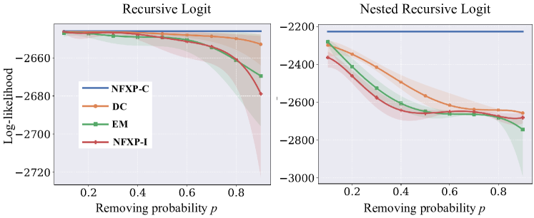
Figure 1: Log-likelihood comparison for the RL and NRL models.

Figure 1 reports the means and standard errors of the LL values given by the four approaches, where the solid curves represent the mean values, and the shaded areas represent the standard errors. We can see that, for both RL and NRL models, the DC always gives higher LL values, as compared to those given by the EM and NFXP-I. The EM seems to be better than NFXP-I in some cases, and worse in some other cases. For the RL model, all the approaches (DC, EM and NFXP-I) seem to perform well as $p$ increases. The gaps between the DC, EM and NFXP-I are small for $p\leq 0.6$ and become more significant when $p\geq 0.7$. This demonstrates the efficiency of the DC algorithm in handling highly incomplete data. For the NRL model, we however see that the DC, EM and NFXP-I seem to perform worse, as compared to the case of the RL model; the LL values drop more quickly as $p$ increases. This is to be expected as we know that the NRL model has more complicated forms and has more information to infer (i.e., the parameters of the link utilities and the scales $\mu_{k}$, $k\in\widetilde{\mathcal{A}}$). We however still see that the DC significantly outperforms the EM and NFXP-I approaches for $p\leq 0.7$ and is slightly better than EM and NFXP-I for $p\geq 0.8$. Moreover, EM is slightly better than NFXP-I for $p\leq 0.5$ and slightly worse than NFXP-I for $p=0.9$.

Model	Removing Probability	EM	DC	NFXP-I
RL	0.0	-2646.08
	0.1	-2646.98$\pm$0.73	-2646.25$\pm$0.18	-2646.43$\pm$0.28
	0.2	-2647.71$\pm$1.51	-2646.40$\pm$0.21	-2646.82$\pm$0.84
	0.3	-2647.77$\pm$1.25	-2646.53$\pm$0.37	-2647.00$\pm$0.72
	0.4	-2649.23$\pm$2.34	-2646.84$\pm$0.36	-2647.77$\pm$1.30
	0.5	-2649.57$\pm$2.74	-2647.29$\pm$0.60	-2649.31$\pm$2.81
	0.6	-2650.58$\pm$1.92	-2648.23$\pm$0.76	-2651.07$\pm$2.88
	0.7	-2654.02$\pm$6.61	-2648.61$\pm$1.45	-2654.83$\pm$7.00
	0.8	-2661.72$\pm$11.03	-2649.97$\pm$2.42	-2660.45$\pm$8.87
	0.9	-2669.37$\pm$17.59	-2652.90$\pm$5.45	-2678.95$\pm$24.05
NRL	0.0	-2162.32
	0.1	-2292.91$\pm$46.48	-2258.39$\pm$62.34	-2361.82$\pm$29.23
	0.2	-2452.83$\pm$42.77	-2379.86$\pm$61.90	-2493.52$\pm$23.33
	0.3	-2545.09$\pm$29.06	-2419.17$\pm$28.45	-2571.09$\pm$20.18
	0.4	-2615.28$\pm$20.70	-2474.93$\pm$24.33	-2625.09$\pm$22.23
	0.5	-2668.62$\pm$28.33	-2528.01$\pm$19.49	-2683.15$\pm$26.50
	0.6	-2728.13$\pm$22.93	-2585.90$\pm$11.48	-2732.94$\pm$27.95
	0.7	-2669.20$\pm$6.99	-2631.07$\pm$17.03	-2656.76$\pm$8.80
	0.8	-2676.56$\pm$8.86	-2652.93$\pm$11.63	-2668.96$\pm$10.79
	0.9	-2827.12$\pm$347.75	-2659.35$\pm$5.79	-2684.21$\pm$18.56

Table 1: Means and standard errors of the LL values (over 10 runs) for the RL and NRL models.

We also report the details of the means and standard errors of the LL values in Table 1, where the values before “$\pm$” are the means and the values after “$\pm$” are the standard errors. The LL values reported for $p=0.0$ are also the LL values given by the NFXP-C (i.e., given by the NFXP with the complete data). It can be seen that the LL values given by the NRL model are significantly higher than those given by the RL model. This is to be expected as previous studies already show that the NRL model always performs better than the RL in terms of in- and out-of-sample fits. Moreover, we see that the standards errors given by the RL are much smaller than those given by the NRL model, for all the three algorithms, which can be explained by the fact that the NRL model yields a more complicated choice probability formulation and is more difficult to estimate. Furthermore, looking at the LL values across the three approaches EM, DC, and NFXP-I, we also see that DC does not only return larger mean LL values, but also yields small LL standard errors. This would be due to the fact that the DC approach computes the probabilities of unconnected segments exactly while the EM algorithm approximates them by sampling, and the NFXP-I simply ignores the missing segments. This observation demonstrates the efficiency and stability of the DC approach, as compared to the other ones.

In summary, our experiments show that DC denominates the other approaches (i.e., EM and NFXP-I) in recovering missing information, in the sense that the LL values given by the DC algorithm are always higher (thus are closer to the ground-truth values), as compared to those given by EM and NFXP-I. Moreover, our approaches seem to provide better results for the RL model than for the NRL model.

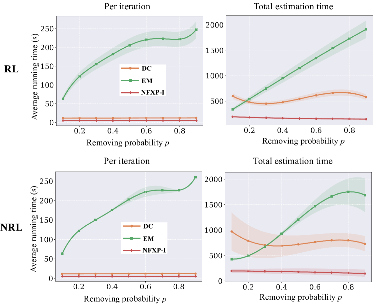
Figure 2: Average running time comparison for the RL and NRL models.

We now turn our attention to the computational costs required to run our algorithms, which is also a focus of this work. In Figure 2 we plot the means (solid curves) and standard errors (shaded areas) of the running times of the three algorithm DC, EM, and NFXP-I, for the RL and NRL models, noting that the running times of NFXP-I and NFXP-C are generally similar. In each figure, the left-hand side reports the average running times per iteration and the right-hand side reports the average total running times. It can be seen that, per iteration, DC and EM are much faster than EM, and as expected, NFXP-I is faster than DC. Importantly, the running times (per iteration) of EM grow quickly as $p$ increases while the running times (per iteration) of DC and NFXP-I are stable. This is because when the removing probability $p$ increases, the dataset would contain more unconnected segments and the EM algorithm would need more samples to approximate the expected LL function, thus becoming more expensive. In contrast, the DC algorithm is developed in such a way that the number of systems of equations to be solved does not depend on the number of unconnected segments in the path observations. The number of linear systems to be solved also does not change as $p$ increases for the NFXP-I algorithm. Thus, an increase in $p$ would not make a significant impact on the running times of DC and NFXP-I.

In terms of total estimation time, it is interesting to see that the EM algorithm is faster than the DC for some small $p$ values (e.g., $p\leq 0.2$ for the RL and $p\leq 0.3$ for the NRL models), even though the running times per iteration of the EM are higher. This would be explained as follows. When $p$ is small, the number of unconnected segments in the observations is small, thus the EM algorithm only requires a small number of path samples and $\widehat{R}({\boldsymbol{\theta}}|{\boldsymbol{\theta}}^{t})$ would give a good approximation to the expected LL function. Moreover, the form of the approximate expected LL function in (7), even though looks complex, it shares a similar structure with the standard LL functions studied in previous works (Fosgerau et al., 2013, Mai et al., 2015). On the other hand, the LL function in the DC approach involves some exact probabilities of unconnected segments, thus would be more complicated. All these would be the reason for the fact that when $p$ is small, EM requires fewer iterations to converge and is faster, as compared to the DC algorithm.

When $p\geq 0.2$ for the RL model and $p\geq 0.3$ for the NRL model, the running times of EM start becoming higher than those of DC and increase fast. This is to be expected as the running times per iteration of EM also increases fast as $p$ increase. The total estimation times of the DC algorithm, as expected, are stable and seem not to be affected much by an increase in $p$. Moreover, looking across the two route choice models, we see that the total running times of DC are higher for the NRL model, as compared to those given by the RL model. This is to be expected as the NRL model is known to be more expensive to estimate than the RL model. However, it seems not to be the case for the EM approach. The standard errors of the running times seem to be higher for the NRL model, which is consistent with our above observations for the LL comparisons. We refer the reader to the appendix for the details of the running times.

In summary, in terms of running time, the DC and EM algorithms are more expensive to perform than the naive approach NFXP-I. The DC algorithm is generally much faster than the EM, especially when $p$ is large. More importantly, the running times of EM grow fast as the data-missing level $p$ increases, while an increase in $p$ does not make a significant impact on the running times of DC. All these indicate the practical tractability of the DC approach for handling highly missing data.

6 Conclusion

In this paper, we have studied the issue of incomplete observations in route choice modeling. we have developed two solution approaches, namely, the EM and DC algorithms, aiming to efficiently recover missing information from data. While the EM algorithm requires to solve several MLE problems and would be expensive to perform, the DC algorithm is based on the idea that we can exactly compute the probabilities of unconnected segments by solving systems of linear equations. The main advantage of our DC algorithm is that the number of system of linear equations to be solved to compute the probabilities of unconnected segments does not depend on the number of unconnected segments, thus this approach scales well when the number of unconnected segments increases. We provide numerical experiments based on a dataset collected from a real network, which showed that the DC algorithm outperforms the EM and other baselines in recovering missing information. Our numerical results also showed that the DC algorithm is generally faster than the EM approach, and the running times of the DC seem not to be affected by the amount of missing information in the data observations.

Our methods can be used with other recursive models developed in the literature, e.g., the dynamic RL (de Moraes Ramos et al., 2020) or stochastic time-dependent RL (Mai et al., 2021) models, and may have applications beyond route choice modeling, for example, the estimation of activity-based models or general structural dynamic discrete choice models with missing data. These would shape some interesting directions for future work.

Appendix

Tables 2 and 3 below report the details of the running times (per iteration and overall) of the three algorithms (EM, DC and NFXP-I). The means are reported before $``\pm^{\prime\prime}$ and the standard errors are reported after $``\pm^{\prime\prime}$. The running times of the NFXP-I are in general small and stable as $p$ increases. It is important to note that, in terms of running time per iteration, the running time standard errors of the DC and NFXP-I are considerably smaller than those of the EM algorithm, but the overall running time standard errors of the DC and NFXP-I are comparable with those of the EM, indicating that the numbers of iterations required by DC and NFXP-I vary significantly across the 10 independent runs.

	Removing probability	EM	DC	NFXP-I
Per iteration	0.1	62.85$\pm$5.66	11.34$\pm$1.02	5.40$\pm$0.49
	0.2	102.16$\pm$9.19	11.49$\pm$1.03	5.61$\pm$0.51
	0.3	141.71$\pm$12.75	11.50$\pm$1.04	5.56$\pm$0.50
	0.4	169.21$\pm$15.23	11.48$\pm$1.03	5.46$\pm$0.49
	0.5	195.89$\pm$17.63	11.52$\pm$1.04	5.50$\pm$0.49
	0.6	214.90$\pm$19.34	11.61$\pm$1.04	5.60$\pm$0.50
	0.7	223.32$\pm$20.10	11.67$\pm$1.05	5.58$\pm$0.50
	0.8	221.64$\pm$19.95	11.67$\pm$1.05	5.42$\pm$0.49
	0.9	228.72$\pm$20.59	11.68$\pm$1.05	5.37$\pm$0.48
Total estimation time	0.1	336.88$\pm$30.32	597.28$\pm$53.76	190.23$\pm$17.12
	0.2	452.45$\pm$40.72	517.06$\pm$46.54	183.30$\pm$16.50
	0.3	650.87$\pm$58.58	452.12$\pm$40.69	173.28$\pm$15.60
	0.4	848.78$\pm$76.39	457.00$\pm$41.13	165.35$\pm$14.88
	0.5	1061.45$\pm$95.53	511.65$\pm$46.05	158.76$\pm$14.29
	0.6	1255.07$\pm$112.96	580.52$\pm$52.25	154.18$\pm$13.88
	0.7	1460.70$\pm$131.46	644.85$\pm$58.04	150.49$\pm$13.54
	0.8	1645.63$\pm$148.11	667.59$\pm$60.08	147.91$\pm$13.31
	0.9	1824.82$\pm$164.23	629.08$\pm$56.62	145.82$\pm$13.12

Table 2: Means and standard errors of the running times (in seconds - over 10 runs), overall estimation time and per iteration, for the RL model.

	Removing probability	EM	DC	NFXP-I
Per iteration	0.1	63.17$\pm$1.03	11.53$\pm$0.00	5.63$\pm$0.36
	0.2	103.30$\pm$2.18	11.52$\pm$0.04	5.54$\pm$0.42
	0.3	138.25$\pm$0.43	11.54$\pm$0.06	5.54$\pm$0.43
	0.4	162.58$\pm$0.13	11.58$\pm$0.06	5.58$\pm$0.40
	0.5	191.02$\pm$5.32	11.61$\pm$0.06	5.59$\pm$0.38
	0.6	214.39$\pm$10.92	11.64$\pm$0.06	5.54$\pm$0.41
	0.7	226.40$\pm$11.60	11.69$\pm$0.06	5.48$\pm$0.48
	0.8	225.55$\pm$5.46	11.75$\pm$0.07	5.44$\pm$0.54
	0.9	235.50$\pm$-1.01	11.79$\pm$0.10	5.44$\pm$0.54
Total estimation time	0.1	428.10$\pm$32.51	972.34$\pm$375.06	197.09$\pm$40.28
	0.2	448.51$\pm$14.83	854.86$\pm$337.80	194.84$\pm$43.20
	0.3	579.70$\pm$4.97	732.59$\pm$280.47	190.68$\pm$49.28
	0.4	797.22$\pm$17.67	688.93$\pm$231.93	186.04$\pm$56.14
	0.5	1082.86$\pm$52.50	701.55$\pm$189.90	180.32$\pm$63.69
	0.6	1348.92$\pm$100.02	741.97$\pm$161.46	174.27$\pm$70.04
	0.7	1591.04$\pm$163.63	787.37$\pm$142.52	166.72$\pm$75.46
	0.8	1728.20$\pm$229.48	804.20$\pm$136.61	158.69$\pm$78.41
	0.9	1740.45$\pm$298.27	771.47$\pm$142.39	149.52$\pm$78.70

Table 3: Means and standard errors of the running times (in seconds - over 10 runs), overall and per iteration, for the NRL model.

References

- Arcidiacono and Miller (2011) Arcidiacono, P. and Miller, R. A. Conditional choice probability estimation of dynamic discrete choice models with unobserved heterogeneity. Econometrica, 79(6):1823–1867, 2011.
- Baillon and Cominetti (2008) Baillon, J.-B. and Cominetti, R. Markovian traffic equilibrium. Mathematical Programming, 111(1-2):33–56, 2008.
- Bierlaire and Frejinger (2008) Bierlaire, M. and Frejinger, E. Route choice modeling with network-free data. Transportation Research Part C, 16(2):187–198, 2008.
- Broach et al. (2012) Broach, J., Dill, J., and Gliebe, J. Where do cyclists ride? a route choice model developed with revealed preference gps data. Transportation Research Part A: Policy and Practice, 46(10):1730–1740, 2012.
- de Moraes Ramos (2015) de Moraes Ramos, G. Dynamic Route Choice Modelling of the Effects of Travel Information using RP Data. Ph.D. thesis, TU Delft, Delft University of Technology, 2015.
- de Moraes Ramos et al. (2020) de Moraes Ramos, G., Mai, T., Daamen, W., Frejinger, E., and Hoogendoorn, S. Route choice behaviour and travel information in a congested network: Static and dynamic recursive models. Transportation Research Part C: Emerging Technologies, 114:681–693, 2020.
- Dempster et al. (1977) Dempster, A. P., Laird, N. M., and Rubin, D. B. Maximum likelihood from incomplete data via the em algorithm. Journal of the Royal Statistical Society: Series B (Methodological), 39(1):1–22, 1977.
- Dill and Gliebe (2008) Dill, J. and Gliebe, J. Understanding and measuring bicycling behavior: A focus on travel time and route choice. In Final report. Oregon Transportation Research and Education Consortium, 2008.
- Fosgerau et al. (2013) Fosgerau, M., Frejinger, E., and Karlström, A. A link based network route choice model with unrestricted choice set. Transportation Research Part B, 56:70–80, 2013.
- Gentle (1998) Gentle, J. The EM algorithm and extensions. Biometrics, 54(1):395, 1998.
- Gilani (2005) Gilani, H. Automatically determine route and mode of tranport using a gps enabled phone. In (Dissertation, the degree of Master of Science in Computer Science). University of South Florida., 2005.
- Krizek et al. (2007) Krizek, K. J., El-Geneidy, A., and Thompson, K. A detailed analysis of how an urban trail system affects cyclists’ travel. Transportation, 34(5):611–624, 2007.
- Mai (2016) Mai, T. A method of integrating correlation structures for a generalized recursive route choice model. Transportation Research Part B: Methodological, 93:146–161, 2016.
- Mai and Frejinger (2022) Mai, T. and Frejinger, E. Estimation of undiscounted recursive path choice models: Convergence properties and algorithms. Forthcoming in Transportation Science, 2022.
- Mai et al. (2015) Mai, T., Fosgerau, M., and Frejinger, E. A nested recursive logit model for route choice analysis. Transportation Research Part B, 75(0):100 – 112, 2015. ISSN 0191-2615.
- Mai et al. (2018) Mai, T., Bastin, F., and Frejinger, E. A decomposition method for estimating recursive logit based route choice models. EURO Journal on Transportation and Logistics, 7(3):253–275, 2018.
- Mai et al. (2021) Mai, T., Yu, X., Gao, S., and Frejinger, E. Route choice in a stochastic time-dependent network: the recursive model and solution algorithm. Transportation Research Part B: Methodological, 151:42, 2021.
- McLachlan et al. (2019) McLachlan, G. J., Lee, S. X., and Rathnayake, S. I. Finite mixture models. Annual review of statistics and its application, 6:355–378, 2019.
- Melo (2012) Melo, E. A representative consumer theorem for discrete choice models in networked markets. Economics Letters, 117(3):862–865, 2012.
- Melville et al. (2004) Melville, P., Shah, N., Mihalkova, L., and Mooney, R. J. Experiments on ensembles with missing and noisy data. In International Workshop on Multiple Classifier Systems, pages 293–302. Springer, 2004.
- Menghini et al. (2010) Menghini, G., Carrasco, N., Schüssler, N., and Axhausen, K. W. Route choice of cyclists in zurich. Transportation research part A: policy and practice, 44(9):754–765, 2010.
- Nocedal and Wright (2006a) Nocedal, J. and Wright, S. J. Numerical Optimization. Springer, New York, NY, USA, 2nd edition, 2006a.
- Nocedal and Wright (2006b) Nocedal, J. and Wright, S. J. Numerical optimization. Springer, New York, NY, USA, 2006b.
- Oliveira and Casas (2010) Oliveira, M. G. S. and Casas, J. Improving data quality, accuracy, and response in on-board surveys: Application of innovative technologies. Transportation research record, 2183(1):41–48, 2010.
- Osorio and Chong (2015) Osorio, C. and Chong, L. A computationally efficient simulation-based optimization algorithm for large-scale urban transportation problems. Transportation Science, 49(3):623–636, 2015.
- Oyama and Hato (2017) Oyama, Y. and Hato, E. A discounted recursive logit model for dynamic gridlock network analysis. Transportation Research Part C: Emerging Technologies, 85:509–527, 2017.
- Papinski et al. (2009) Papinski, D., Scott, D. M., and Doherty, S. T. Exploring the route choice decision-making process: A comparison of planned and observed routes obtained using person-based gps. Transportation research part F: traffic psychology and behaviour, 12(4):347–358, 2009.
- Paszke et al. (2019) Paszke, A., Gross, S., Massa, F., Lerer, A., Bradbury, J., Chanan, G., Killeen, T., Lin, Z., Gimelshein, N., Antiga, L., et al. Pytorch: An imperative style, high-performance deep learning library. Advances in neural information processing systems, 32, 2019.
- Prato (2009) Prato, C. G. Route choice modeling: past, present and future research directions. Journal of Choice Modelling, 2:65–100, 2009.
- Prato (2012) Prato, C. G. Estimating random regret minimization models in the route choice context. In Proceedings of the 13th International Conference on Travel Behaviour Research, Toronto, Canada, 2012.
- Rust (1987) Rust, J. Optimal replacement of GMC bus engines: An empirical model of Harold Zurcher. Econometrica, 55(5):999–1033, 1987.
- Shen and Stopher (2014) Shen, L. and Stopher, P. R. Review of GPS travel survey and GPS data-processing methods. Transport Reviews, 34(3):316–334, 2014.
- Smith et al. (2003) Smith, B. L., Scherer, W. T., and Conklin, J. H. Exploring imputation techniques for missing data in transportation management systems. Transportation Research Record, 1836(1):132–142, 2003.
- Wang et al. (2011) Wang, Y., Zhu, Y., He, Z., Yue, Y., and Li, Q. Challenges and opportunities in exploiting large-scale GPS probe data. HP Laboratories, Technical Report HPL-2011-109, 21, 2011.
- Wolf et al. (1999) Wolf, J., Hallmark, S., Oliveira, M., Guensler, R., and Sarasua, W. Accuracy issues with route choice data collection by using global positioning system. Transportation Research Record, 1660(1):66–74, 1999.
- Zimmermann and Frejinger (2020) Zimmermann, M. and Frejinger, E. A tutorial on recursive models for analyzing and predicting path choice behavior. EURO Journal on Transportation and Logistics, 9(2):100004, 2020.
- Zimmermann et al. (2021) Zimmermann, M., Frejinger, E., and Marcotte, P. A strategic markovian traffic equilibrium model for capacitated networks. Transportation Science, 55(3):574–591, 2021.