Abstract

Neal and Hinton (1998) recast maximum likelihood estimation of any given latent variable model as the minimization of a free energy functional $F$, and the EM algorithm as coordinate descent applied to $F$. Here, we explore alternative ways to optimize the functional. In particular, we identify various gradient flows associated with $F$ and show that their limits coincide with $F$’s stationary points. By discretizing the flows, we obtain practical particle-based algorithms for maximum likelihood estimation in broad classes of latent variable models. The novel algorithms scale to high-dimensional settings and perform well in numerical experiments.

1 INTRODUCTION

In machine learning and statistics, we often use a probabilistic model, $p_{\theta}(x,y)$, defined in terms of a vector of parameters, $\theta$, to infer some quantities, $x$, that we cannot observe experimentally from some, $y$, that we can. A pragmatic middle ground between Bayesian and frequentist approaches to this type of problem is the empirical Bayes (EB) paradigm (Robbins, 1956) wherein we

1. learn the parameters from the data: we search for parameters $\theta_{*}$ that explain the data $y$ well;

2. use $\theta_{*}$ to infer, and quantify the uncertainty in, $x$.

Because this approach does not require eliciting a prior over the parameters, it is particularly appealing for models whose parameters lack physical interpretations or meaningful prior information; e.g. the generator network in Sec. 3.3. Steps (S1,2) are typically reformulated technically as

1. find a $\theta_{*}$ maximizing the marginal likelihood,

   $$p_{\theta}(y):=\int p_{\theta}(x,y)dx;$$

2. obtain the corresponding posterior distribution,

   $$p_{\theta_{*}}(x|y):=\frac{p_{\theta_{*}}(x,y)}{p_{\theta_{*}}(y)}.$$

Perhaps the most well-known method for tackling (S1,2) is the expectation maximization (EM) algorithm (Dempster et al., 1977): starting from an initial guess $\theta_{0}$, alternate,

1. compute $q_{k}:=p_{\theta_{k}}(\cdot|y)$,

2. solve for $\theta_{k+1}:=\operatorname*{arg\,max}_{\theta\in\Theta}\int\ell(\theta,x)q_{k+1}(x)dx$,

where $\ell(\theta,x):=\log(p_{\theta}(x,y))$ denotes the log-likelihood. Under general conditions (McLachlan, 2007, Chap. 3), $\theta_{k}$ converges to a stationary point $\theta_{*}$ of the marginal likelihood and $q_{k}$ to the corresponding posterior $p_{\theta_{*}}(\cdot|y)$. In cases where the above steps are not analytically tractable, it is common to approximate (E) using Monte Carlo (or Markov chain Monte Carlo if $p_{\theta}(\cdot|y)$ cannot be sampled directly) and (M) using numerical optimization (e.g. with a single gradient or Newton step in Euclidean spaces); cf. Wei and Tanner (1990); Kuk and Cheng (1997); Delyon et al. (1999); Younes (1999); Kuhn and Lavielle (2004); Han et al. (2017); Qiu and Wang (2020); Cai (2010); Nijkamp et al. (2020); De Bortoli et al. (2021).

Here, we take a different approach that builds on an insightful observation made by Neal and Hinton (1998) (see Csiszár and Tusnády (1984) for a precedent): EM can be recast as a well-known optimization routine applied to a certain objective. The objective is the ‘free energy’:

$$F(\theta,q): =\int\log(q(x))q(x)dx-\int\ell(\theta,x)q(x)dx$$ (1)

for all $(\theta,q)$ in $\Theta\times\mathcal{P}(\mathcal{X})$, where $\Theta$ denotes the parameter space and $\mathcal{P}(\mathcal{X})$ the space of probability distributions over the latent space $\mathcal{X}$. The optimization routine is coordinate descent: starting from an initial guess $\theta_{0}$, alternate,

1. solve for $q_{k}:=\operatorname*{arg\,min}_{q\in\mathcal{P}(\mathcal{X})}F(\theta_{k},q)$,

2. solve for $\theta_{k+1}:=\operatorname*{arg\,min}_{\theta\in\Theta}F(\theta,q_{k})$.

The key here is the following result associating the maxima of $p_{\theta}(y)$ with the minima of $F$:

Theorem 1.

For any $\theta$ in $\Theta$, the posterior $p_{\theta}(\cdot|y):=p_{\theta}(\cdot,y)/p_{\theta}(y)$ minimizes $q\mapsto F(\theta,q)$. Moreover, $p_{\theta}(y)$ has a global maximum at $\theta$ if and only if $F$ has a global minimum at $(\theta,p_{\theta}(\cdot|y))$.

The theorem follows easily from the same type of arguments as those used to prove Neal and Hinton (1998, Lem. 1, Thrm. 2). Similar statements can also be made for local optima, but we refrain from doing so here because it involves specifying what we mean by ‘local’ in $\Theta\times\mathcal{P}(\mathcal{X})$. The point is that finding a maximum of $p_{\theta}(y)$ and computing the corresponding posterior is equivalent to finding a minimum of $F$, and this is precisely what EM does. It has the same drawback as coordinate descent: we must be able to carry out the coordinate descent steps (or, equivalently, the EM steps) exactly. Consequently, at least in its original presentation, EM is limited to relatively simple models.

For more complex models, it is natural to ask: ‘Could we instead solve (S1,2) by applying a different optimization routine to $F$? What about perhaps the most basic of them all, gradient descent?’. To affirmatively answer both questions, we need (a) a sensible notion of a ‘gradient’ for functionals on $\Theta\times\mathcal{P}(\mathcal{X})$ and (b) practical methods implementing the gradients steps, at least approximately. At the time of Neal and Hinton (1998)’s publication, these obstacles had already begun to crumble: Otto and coworkers had introduced (Jordan et al., 1998; Otto, 2001) a notion of gradients for functionals on $\mathcal{P}(\mathcal{X})$ (w.r.t. to the Wasserstein-2 geometry) and an associated calculus; and Ermak (1975); Parisi (1981) had proposed the unadjusted Langevin algorithm (ULA, name coined in Roberts and Tweedie (1996)) that turned out to be a practical Monte Carlo approximation of the corresponding gradient descent algorithm applied to a particular functional (although this connection has only been fleshed out much more recently in papers such as Cheng and Bartlett (2018)). In the ensuing two decades, these two lines of work have progressed greatly: Otto et al.’s ideas have been consolidated and imbued with rigour (Villani, 2009; Ambrosio et al., 2005), analogues have been established for other geometries on $\mathcal{P}(\mathcal{X})$ (Duncan et al., 2019; Garbuno-Inigo et al., 2020; Lu et al., 2019), and more practical methods have been published (Liu and Wang, 2016; Garbuno-Inigo et al., 2020; Lu et al., 2019; Reich and Weissmann, 2021; Chen et al., 2018).

Here, we capitalize on these developments and obtain scalable, easy-to-implement algorithms that tackle (S1,2) for broad classes of models (any for which $\Theta$ and $\mathcal{X}$ are euclidean and the density $p_{\theta}(x,y)$ is differentiable in $\theta$ and $x$). We consider three methods: an approximation to gradient descent (Sec. 2), one to Newton’s method (App. C), and a further ‘marginal gradient’ method (App. D) applicable to models for which the (M) step is tractable but the (E) step is not — a surprisingly common situation in practice. We then study their performance in three examples (Sec. 3). We conclude with a discussion of our methods, their limitations, and future research directions (Sec. 4). Code for our examples can be found at https://github.com/juankuntz/ParEM.

Related literature and contributions.

Procedures reminiscent of those in Sec. 2 and Apps. C, D are commonplace in variational inference, e.g. see Kingma and Welling (2019, Sec. 2). Here, practitioners choose a tractable parametric family $\mathcal{Q}:=(q_{\phi})_{\phi\in\Phi}\subseteq\mathcal{P}(\mathcal{X})$, parametrized by $\phi$s in some set $\Phi$, and solve

$$(\theta_{*},\phi_{*})=\operatorname*{arg\,min}_{(\theta,\phi)\in\Theta\times\Phi}F(\theta,q_{\phi})$$ (2)

using an appropriate optimization algorithm. If $\mathcal{Q}$ is sufficiently rich, then $(\theta_{*},q_{\phi_{*}})$ will be close to an optimum of $(\theta,q)\mapsto F(\theta,q)$ if $(\theta_{*},\phi_{*})$ is an optimum of $(\theta,\phi)\mapsto F(\theta,q_{\phi})$. How rich $\mathcal{Q}$ needs to be is a complicated question and, in practice, $\mathcal{Q}$’s choice is usually dictated by computational considerations. Because the optimization of interest is that of $(\theta,q_{\phi})$ over $\Theta\times\mathcal{Q}$ rather than that of $(\theta,\phi)$ over $\Theta\times\Phi$, it often proves beneficial to adapt the optimization routine appropriately. For instance, one could use natural gradients (Martens, 2020) defined not w.r.t. the Euclidean geometry on $\Phi$ but instead w.r.t. a geometry that accounts for the effect that changes in $\phi$ have in $q_{\phi}$, with changes in $q_{\phi}$ measured by the KL divergence. In this paper, we circumvent these issues by working directly in $\mathcal{P}(\mathcal{X})$. We are also guided by similar considerations when choosing $\theta$ updates (see Apps. C, D in particular): the object of interest here is the distribution $p_{\theta}(\cdot,y)$ indexed by $\theta$ rather than $\theta$ itself (but, $p_{\theta}(\cdot,y)$ is unnormalized, and it is no longer obvious that natural gradients are sensible).

Well-known algorithms are corner cases of ours. If the parameter space is trivial ($\Theta=\{\theta\}$) and we use a single particle ($N=1$ in what follows), the methods in Sec. 2 and Apps. C, D reduce to ULA applied to the unnormalized density $p_{\theta}(\cdot,y)$. If, on the other hand, the latent space is trivial, the algorithm in Sec. 2 collapses to gradient descent applied to $\theta\mapsto p_{\theta}(y)$ and that in App. C to Newton’s method. Lastly, although we find the EB setting a natural one for introducing our methods, the EM algorithm can also be used to tackle many other problems, e.g. see McLachlan (2007, Chap. 8), and, subject to the limitations discussed in Sec. 4, so can ours.

The contributions of this paper are as follows:

1. We identify various gradient flows associated with $F$ (Sec. 2, Apps. C, D), review the pertinent theory (App. A), and provide theoretical evidence for their convergence to $F$’s optima (Thrm. 3, App. B.2).

2. Building on the insights afforded by (1), we derive three novel particle-based alternatives to EM (Sec. 2, Apps. C, D), study them theoretically (Sec. 2, Apps. G, F), consider modifications that enhance their practical utility (Secs. 2, 3.3), and demonstrate the latter via several examples (Sec. 3).

3. We pave the way to other novel methods for maximum likelihood estimation in latent variable models (Sec. 4), be they, for example, optimization-inspired ones like those in Sec. 2 and Apps. C, D or pure Monte Carlo approaches like those in App. H.

Our setting, notation, assumptions, rigour, and lack thereof.

In this methodological paper, we favour intuition and clarity of presentation over mathematical rigour. We believe that all of the statements we make can be argued rigorously under the appropriate technical conditions, but we do not dwell on what these are. Except where strictly necessary, we avoid measure-theoretic notation, and we commit the usual notational abuse of conflating measures and kernels with their densities w.r.t. to the Lebesgue measure (this can be remedied by interpreting equations weakly and replacing density ratios with Radon-Nikodym derivatives). We also focus on Euclidean parameter and latent spaces ($\Theta=\mathbb{R}^{D_{\theta}}$ and $\mathcal{X}=\mathbb{R}^{D_{x}}$ for $D_{\theta},D_{x}>0$), although our results and methods apply almost unchanged were these to be differentiable Riemannian manifolds. Throughout, $\bm{1}_{d}$ and $I_{d}$ respectively denote the $d$-dimensional vector of ones and identity matrix, $\mathcal{N}(\mu,\Sigma)$ the normal distribution with mean vector $\mu$ and covariance matrix $\Sigma$, and $\mathcal{N}(x;\mu,\Sigma)$ its density evaluated at $x$. We also tacitly assume that $p_{\theta}(x,y)>0$ for all $\theta,x,$ and $y$; and that $(\theta,x)\mapsto p_{\theta}(x,y)$ is sufficiently regular that any gradients or Hessians we use are well-defined and any integral-derivative swaps and applications of integration-by-parts we do are justified. Furthermore, we make the following assumption, the violation of which indicates a poorly parametrized model or insufficiently informative data.

Assumption 1.

The marginal likelihood’s super-level sets $\{\theta\in\Theta:p_{\theta}(y)\geq l\}$, for any $l>0$, are bounded.

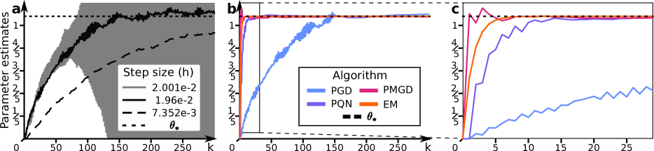
Figure 1: Toy hierarchical model. Parameter estimates for Ex. 1 with $D_{x}=100$ latent variables, $N=10$ particles, and both particles and estimates initialized at zero. a PGD estimates $\theta_{k}$ for three step sizes $h$. b PGD, PQN, PMGD, and EM parameter estimates. EM converges without averaging over time. For PGD, PQN, and PMGD, we use optimal step sizes (respectively, $h=1/51,2/3,1$, cf. App. F.1) and start averaging once the estimates reach stationarity (i.e. plot shows $\theta_{k}$ for $k<k_{b}$ and $\bar{\theta}_{k}$ for $k\geq k_{b}$ with $k_{b}=150,15,5$ for PGD, PQN, PMGD, respectively). c First $30$ steps in b.

2 PARTICLE GRADIENT DESCENT

The basic gradient descent algorithm for minimizing a differentiable function $f:\mathbb{R}^{n}\to\mathbb{R}$,

$$x_{k+1}=x_{k}-h\nabla_{x}f(x_{k}),$$ (3)

is the Euler discretization with step size $h>0$ of $f$’s continuous-time gradient flow $\dot{x}_{t}=-\nabla_{x}f(x_{t})$, where $\nabla_{x}$ denotes the usual Euclidean gradient w.r.t. to $x$. To obtain an analogue of (3) applicable to $F$ in (1), we identify an analogue of $f$’s gradient flow and discretize it. Here, we require a sensible notion for $F$’s gradient. We use $\nabla F(\theta,q)=(\nabla_{\theta}F(\theta,q),\nabla_{q}F(\theta,q))$, where

$$\nabla_{\theta}F(\theta,q) =-\int\nabla_{\theta}\ell(\theta,x)q(x)dx,$$ (4)

$$\nabla_{q}F(\theta,q) =\nabla_{x}\cdot\left[q\nabla_{x}\log\left(\frac{p_{\theta}(\cdot,y)}{q}\right)\right].$$ (5)

This is the gradient obtained if we endow $\Theta$ with the Euclidean geometry and $\mathcal{P}(\mathcal{X})$ with the Wasserstein-2 one (see App. B.1). It vanishes if and only if $\theta$ is a stationary point of $p_{\theta}(y)$ and $q$ is its corresponding posterior:

Theorem 2 ($1^{st}$ order optimality condition).

$\nabla F(\theta,q)=0$ if and only if $\nabla_{\theta}p_{\theta}(y)=0$ and $q=p_{\theta}(\cdot|y)$.

Proof.

Examining (4,5) we see that $\nabla_{q}F(\theta,q)=0$ if and only if $q\propto p_{\theta}(\cdot,y)$. Given that $q$ is a probability distribution, it follows that $\nabla_{q}F(\theta,q)=0$ if and only if $q=p_{\theta}(\cdot|y)$. The result then follows from

$$\nabla_{\theta}p_{\theta}(y) =\int\nabla_{\theta}p_{\theta}(x,y)dx=\int\nabla_{\theta}\ell(\theta,x)p_{\theta}(x,y)dx$$

$$=p_{\theta}(y)\int\nabla_{\theta}\ell(\theta,x)p_{\theta}(x|y)dx$$ (6)

$$=-p_{\theta}(y)\nabla_{\theta}F(\theta,p_{\theta}(\cdot|y)).$$

       ∎ The gradient flow corresponding to (4,5) reads

$$\dot{\theta}_{t} =\int\nabla_{\theta}\ell(\theta_{t},x)q_{t}(x)dx,$$ (7)

$$\dot{q}_{t} =\nabla_{x}\cdot\left[q_{t}\nabla_{x}\log\left(\frac{q_{t}}{p_{\theta_{t}}(\cdot,y)}\right)\right].$$ (8)

Given Assumpt. 1 and Thrm. 2, we expect that an extension of LaSalle’s principle (Carrillo et al., 2020, Thrm. 1) will show that, as $t$ tends to infinity, $\theta_{t}$ approaches a stationary point $\theta_{*}$ of $\theta\mapsto p_{\theta}(y)$ and $q_{t}$ the corresponding posterior $p_{\theta_{*}}(\cdot|y)$; see App. B.2 for more on this. Here, we settle for exponential convergence in the strongly log-concave case:

Theorem 3.

Suppose there exists $\lambda>0$ and $C>0$ s.t.

$$\nabla^{2}\ell(\theta,x)\preceq-\lambda I_{D_{x}+D_{\theta}},\quad\left|\left|{\nabla_{\theta}\ell(\theta,x)}\right|\right|\leq C$$

for all $(\theta,x)$ in $\Theta\times\mathcal{X}$. The marginal likelihood $\theta\mapsto p_{\theta}(y)$ has a unique maximizer $\theta_{*}$ and there exists $C^{\prime}>0$ s.t.

$$\left|\left|{\theta_{t}-\theta_{*}}\right|\right|\leq C^{\prime}e^{-\lambda t}\enskip\text{and}\enskip\left|\left|{q_{t}-p_{\theta_{*}}(\cdot|y)}\right|\right|_{L^{1}}\leq C^{\prime}e^{-\lambda t}$$

for all $t\geq 0$.

See App. B.3 for a proof. Eqs. (7,8) can rarely be solved analytically. To overcome this, note that (7,8) is a mean-field Fokker-Planck equation satisfied by the law of a McKean-Vlasov SDE (Chaintron and Diez, 2022, Sec. 2.2.2):

$$d\theta_{t} =\left[\int\nabla_{\theta}\ell(\theta_{t},x)q_{t}(x)dx\right]dt,$$ (9)

$$dX_{t} =\nabla_{x}\ell(\theta_{t},X_{t})dt+\sqrt{2}dW_{t},$$ (10)

where $q_{t}$ denotes $X_{t}$’s law and $(W_{t})_{t\geq 0}$ a $D_{x}$-dimensional Brownian motion. To obtain an implementable algorithm, we now require a tractable approximation to the integral in (9) and a discretization of the time axis. For the former, we use a finite-sample approximation to $q_{t}$: we generate $N\geq 1$ particles $X^{1}_{t},\dots,X^{N}_{t}$ with law $q_{t}$ by solving

$$dX_{t}^{n}=\nabla_{x}\ell(\theta_{t},X_{t}^{n})dt+\sqrt{2}dW_{t}^{n}\quad\forall n\in[N],$$ (11)

with $[N]:=\{1,\dots,N\}$ and $(W_{t}^{1})_{t\geq 0},\dots,(W_{t}^{N})_{t\geq 0}$ denoting $N$ independent Brownian motions, and exploit

$$q_{t}\approx\frac{1}{N}\sum_{n=1}^{N}\delta_{X_{t}^{n}}$$ (12)

$$\Rightarrow\quad\int\nabla_{\theta}\ell(\theta_{t},x)q_{t}(x)dx\approx\frac{1}{N}\sum_{n=1}^{N}\nabla_{\theta}\ell(\theta_{t},X_{t}^{n}),$$

where $\delta_{x}$ denotes a Dirac delta at $x$. We then obtain the following approximation to (9,11):

$$d\theta_{t} =\left[\frac{1}{N}\sum_{n=1}^{N}\nabla_{\theta}\ell(\theta_{t},X_{t}^{n})\right]dt,$$

$$dX_{t}^{n} =\nabla_{x}\ell(\theta_{t},X_{t}^{n})dt+\sqrt{2}dW_{t}^{n}\enskip\forall n\in[N].$$

To obtain an implementable algorithm (PGD in Alg. 1), we discretize the above using the Euler-Maruyama scheme.

After running PGD for a large enough number of steps $K$, we approximate a stationary point $\theta_{*}$ of the marginal likelihood $\theta\mapsto p_{\theta}(y)$ and its corresponding posterior $p_{\theta_{*}}(\cdot|y)$ with either (a) the final parameter estimates $\theta_{K}$ and the final particle cloud’s empirical distribution $q_{K}=N^{-1}\sum_{n=1}^{N}\delta_{X_{K}^{n}}$; or (b) with time-averaged versions thereof:

$$\bar{\theta}_{K}:=\frac{1}{(K-k_{b})}\sum_{k=k_{b}+1}^{K}\theta_{k},\enskip\bar{q}_{K}:=\frac{1}{(K-k_{b})}\sum_{k=k_{b}+1}^{K}q_{k},$$ (13)

where $k_{b}$ denotes the number of steps discarded as burn-in.

1:  Inputs: step size $h$, step number $K$, particle number $N$, and initial particles $X^{1}_{0},\dots,X_{0}^{N}$ & parameters $\theta_{0}$.

2:  for $k=0,\dots,K-1$ do

3:     Update the parameter estimates:

$$\theta_{k+1}=\theta_{k}+\frac{h}{N}\sum_{n=1}^{N}\nabla_{\theta}\ell(\theta_{k},X_{k}^{n}).$$ (14)

4:     Update the particles: for all $n=1,\dots,N$,

$$X_{k+1}^{n}=X_{k}^{n}+h\nabla_{x}\ell(\theta_{k},X_{k}^{n})+\sqrt{2h}W_{k}^{n},$$ (15)

with $W_{k}^{1},\dots,W_{k}^{N}$ denoting i.i.d. $\mathcal{N}(0,I_{D_{x}})$ R.V.s.

5:  end for

6:  return  $(\theta_{k},q_{k}:=N^{-1}\sum_{n=1}^{N}\delta_{X_{k}^{n}})_{k=0}^{K}$.

Algorithm 1 Particle gradient descent (PGD).

PGD’s behavior.

Given the analogy between (3) and (14,15), we can formulate conjectures for PGD’s behaviour based on that of (stochastic) gradient descent (note that (14) involves noisy estimates of $F$’s $\theta$-gradient) and Thrm. 2:

1. If the step size $h$ is set too large, $\theta_{k}$ will be unstable.

2. Otherwise, after a transient phase, $\theta_{k}$ will hover around a stationary point $\theta_{*}$ of $\theta\mapsto p_{\theta}(y)$, $q_{k}$ around the corresponding posterior $p_{\theta_{*}}(\cdot|y)$, and $(\bar{\theta}_{k},\bar{q}_{k})$ will converge to $(\theta_{*},p_{\theta_{*}}(\cdot|y))$.

3. Small step sizes lead to long transient phases but low estimator variance in the stationary phase.

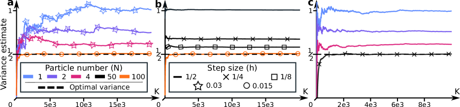
Figure 2: Toy hierarchical model, bias. PMGD estimates for the posterior variance in the $D_{x}=1$ case using the time-averaged posterior approximation $\bar{q}_{K}$ and no burn-in ($k_{b}=0$), as a function of step number $K$. (a) Even with a small step size $h$, using a single particle leads to a significant bias (blue). Growing the particle number $N$ reduces the bias (purple, magenta). The bias becomes negligible for small $h$ and large $N$ (orange). (b) Even with a large $N$, a large $h$ leads to significant bias (solid). Decreasing $h$ reduces the bias (crosses, squares, circles). (c) Adding an accept-reject step removes (B1) regardless of the $h$ employed, and the remaining bias can be removed by choosing a sufficiently large $N$.

Modulo the bias we discuss at the end of this section, (C1–3) are what we observe in our experiments:

Example 1.

Consider a toy hierarchical model involving a single scalar unknown parameter $\theta$, $D_{x}$ i.i.d.  mean-$\theta$ unit-variance Gaussian latent variables, and, for each of these, an independent observed variable with unit-variance Gaussian law centred at the latent variable:

$$p_{\theta}(x,y):=\prod_{d=1}^{D_{x}}\frac{1}{2\pi}\exp\left(-\frac{(x_{d}-\theta)^{2}}{2}-\frac{(y_{d}-x_{d})^{2}}{2}\right).$$

It is straightforward to verify that the marginal likelihood $\theta\mapsto p_{\theta}(y)$ has a unique maximum, $\theta_{*}=D_{x}^{-1}\sum_{d=1}^{D_{x}}y_{d}$, and obtain expressions for the corresponding posterior (see App. E.1). Running PGD, we find that $\theta_{k}$ is unstable if the step size $h$ is too large (Fig. 1a, grey). If $h$ is chosen well, $\theta_{k}$ approaches $\theta_{*}$ and hovers around it (Fig. 1a, black solid) in such a way $\bar{\theta}_{k}$ converges to it (Fig. 1b, blue). If $h$ is too small, the convergence is slow (Fig. 1a, black dashed).

Table 1: Bayesian logistic regression. Test errors achieved using time-averaged posterior approximation $\bar{q}_{400}$, with $N=1,10,100$, and corresponding computation times (averaged over $100$ replicates).

	$N=1$		$N=10$		$N=100$
	Error (%)	Time (s)	Error (%)	Time (s)	Error (%)	Time (s)
PGD	3.58 $\pm$ 0.78	0.03 $\pm$ 0.01	3.55 $\pm$ 0.60	0.09 $\pm$ 0.01	3.46 $\pm$ 0.32	1.22 $\pm$ 0.34
PQN	3.54 $\pm$ 0.77	0.03 $\pm$ 0.00	3.49 $\pm$ 0.60	0.09 $\pm$ 0.00	3.47 $\pm$ 0.33	1.17 $\pm$ 0.26
PMGD	3.56 $\pm$ 0.69	0.03 $\pm$ 0.00	3.65 $\pm$ 0.68	0.09 $\pm$ 0.01	3.44 $\pm$ 0.33	1.15 $\pm$ 0.18
SOUL	3.53 $\pm$ 0.72	0.03 $\pm$ 0.00	3.60 $\pm$ 0.60	0.25 $\pm$ 0.01	3.43 $\pm$ 0.35	13.4 $\pm$ 0.23

Computational complexity and stochastic gradients.

PGD’s complexity is $\mathcal{O}(KN[\text{eval. cost of }(\nabla_{\theta}\ell,\nabla_{x}\ell)])$. We can mitigate the $N$ factor by vectorizing computations across particles. In big data settings where evaluating $\ell$’s gradients is expensive, we replace them with stochastic estimates thereof similarly as in (Robbins and Monro, 1951; Welling and Teh, 2011); cf.  Sec. 3.3 for an example.

Ill-conditioning, a heuristic, adaptive step sizes, PQN, and PMGD.

For many models, each component of $\nabla_{\theta}\ell$ is a sum of $D\gg 1$ terms and, consequently, takes large values. On the other hand, each component of $\nabla_{x}\ell$ typically involves far fewer terms (for instance, two in Ex. 1 while $D=D_{x}$). Hence, the parameter updates in (14) are often much larger steps than the particle updates in (15). This ill-conditioning forces us to use small step sizes $h$ to keep $\theta_{k}$ stable. This results in ‘poor mixing’ for the particles and overall slow convergence. In our experiments, we found that a simple heuristic mitigates the issue: in the parameter update, divide each component of $\nabla_{\theta}\ell$ by the corresponding number of terms ($D_{x}$ in Ex. 1, see Sec. 3.2 for another example). This amounts to pre-multiplying $\nabla_{\theta}\ell$ in (14) by positive definite matrix $\Lambda$ and does not alter (14)’s fixed points. That is, we replace (14) with

$$\theta_{k+1}=\theta_{k}+\frac{h}{N}\sum_{n=1}^{N}\Lambda\nabla_{\theta}\ell(\theta_{k},X_{k}^{n}).$$ (16)

For models with varying time-scales within the $\theta$-components, we found it helpful to adapt $\Lambda$ with $k$ similarly as in Adagrad or RMSProp (e.g., cf. Ruder (2016)); see Sec. 3.3 for an example. In cases where inverting $\ell$’s $\theta$-Hessian is not prohibitively expensive, we can alternatively mitigate the ill-conditioning using the PQN algorithm in App. C. (Indeed, for some simple models, (16,15) coincides with PQN; in more complicated ones, it can be viewed as a crude approximation thereof.) Lastly, in cases where the E step is tractable, we can circumvent this issue with the PMGD algorithm in App. D.

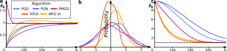
Figure 3: Bayesian logistic regression. a Parameter estimates $\theta_{k}$ initialized at zero (as in De Bortoli et al. (2021)). For PGD, PQN, PMGD, and SOUL, we use $N=100$ particles and a step size of $h=0.01$. b KDE of the second coordinate of the posterior approximation $100^{-1}\sum_{n=1}^{100}X_{400}^{n}$ for PGD, PQN, PMGD, and SOUL, and corresponding marginal of the VI approximation. c As in a, but with estimates initialized at ten.

The bias.

For PGD, PQN, and PMGD, (C2) above is not quite true: the estimates produced by the algorithms are biased in the sense that $(\bar{\theta}_{k},\bar{q}_{k})$ does not converge exactly to $(\theta_{*},p_{\theta_{*}}(\cdot|y))$, but rather to a point in its vicinity. This bias stems from two sources:

1. $\bm{h>0}$. Euler-Maruyama discretizations of the Langevin diffusion do not preserve stationary distributions: this can be seen by examining the mean-field limits of (14,15), cf. App. F.

2. $\bm{N<\infty}$. Our use of finite particle populations: this is best understood by studying the continuum limits of (14,15), cf. App. G.

B1 can be mitigated by decreasing the step size and B2 by increasing the particle number:

Example 2.

Consider again Ex. 1. In this simple case, (B1,2) do not feature in the $\theta$-estimates (Fig. 1) because the model ‘is linear in $\theta$’, cf. App. G.1. To observe (B1,2), we must examine the model’s ‘non-linear aspects’; for instance, the posterior variance whose estimates are biased (Fig. 2).

Of course, increasing $N$ grows the algorithm’s cost, and excessively lowering $h$ slows its convergence. It also seems possible to eliminate (B1) altogether by adding population-wide accept-reject steps as described in App. H, see Fig. 2c. However, we do not dwell on this approach because a practical downside limits its scalability: the acceptance probability degenerates for large $D_{x}$ and $N$, forcing small choices of $h$ and slow convergence.

Table 2: Bayesian neural network. Test errors achieved using the final particle cloud $X_{500}^{1},\dots,X_{500}^{N}$, with $N=1,10,100$, and corresponding computation times (averaged over $10$ replicates).

	$N=1$		$N=10$		$N=100$
	Error (%)	Time (s)	Error (%)	Time (s)	Error (%)	Time (s)
PGD	7.45 $\pm$ 2.03	4.10 $\pm$ 0.26	3.20 $\pm$ 1.12	10.4 $\pm$ 1.2	2.45 $\pm$ 0.99	76.6 $\pm$ 0.4
PQN	7.45 $\pm$ 1.60	4.12 $\pm$ 0.21	3.45 $\pm$ 1.04	10.0 $\pm$ 0.2	2.34 $\pm$ 0.81	74.0 $\pm$ 0.3
PMGD	7.24 $\pm$ 1.75	3.27 $\pm$ 0.13	3.75 $\pm$ 1.38	9.12 $\pm$ 0.2	2.45 $\pm$ 0.81	72.1 $\pm$ 0.5
SOUL	6.25 $\pm$ 1.54	5.02 $\pm$ 0.20	7.25 $\pm$ 1.38	36.5 $\pm$ 0.1	6.85 $\pm$ 1.42	364.0 $\pm$ 5.3

3 NUMERICAL EXPERIMENTS

We examine the performance of our methods by applying them to train a Bayesian logistic regression model for breast cancer prediction (Sec. 3.1), a Bayesian neural network for MNIST classification (Sec. 3.2), and a generator network for image reconstruction and synthesis (Sec. 3.3).

3.1 Bayesian logistic regression

We consider the set-up described in De Bortoli et al. (2021, Sec. 4.1) and employ the same dataset with $683$ datapoints, cf. App. E.2 for details. The latent variables are the $9$ regression weights. We assign an isotropic Gaussian prior $\mathcal{N}(\theta\bm{1}_{D_{x}},5I_{D_{x}})$ to the weights, and we estimate the marginal likelihood’s unique maximizer $\theta_{*}$ (cf. Prop. 1 in App. E.2 for the uniqueness).

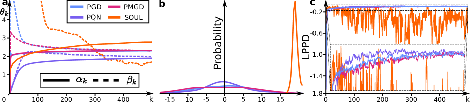
Figure 4: Bayesian neural network. a Parameter estimates as a function of $k$ with $N=100$ particles and step size of $h=0.1$. b KDE of a randomly-chosen coordinate of the posterior approximation $100^{-1}\sum_{n=1}^{100}X_{500}^{n}$. c Log pointwise predictive density as a function of $k$. c, inset c zoomed-in to y-axis range $[-0.16,-0.08]$.

We benchmark our algorithms against the Stochastic Optimization via Unadjusted Langevin (SOUL) algorithm, recently proposed (De Bortoli et al., 2021) to overcome the limited scalability of traditional MCMC EM variants. Because it is a coordinate-wise cousin of PGD (Alg. 1), it allows for straightforward meaningful comparisons with our methods. SOUL approximates the (M) step by updating the parameter estimates using a single (stochastic) gradient step as we do in (14). For the (E) step, it instead runs a single ULA chain for $N$ steps, ‘warm-started’ using the previous chain’s final state ($X_{k}^{1}:=X_{k-1}^{N}$): for all $n\leq N-1$,

$$X_{k}^{n+1}=X_{k}^{n}+h\nabla_{x}\ell(\theta_{k},X_{k}^{n})+\sqrt{2h}W_{k}^{n};$$ (17)

and then approximates $p_{\theta_{k}}(\cdot|y)$ using the chain’s empirical distribution $q_{k}:=N^{-1}\sum_{n=1}^{N}\delta_{X_{k}^{n}}$.

The parameter estimates produced by PGD, PQN (App. C), PMGD (App. D), and SOUL all converge to the same limit (Fig. 3a). SOUL is known (De Bortoli et al., 2021) to return accurate estimates of $\theta_{*}$ for this example, so we presume that this limit approximately equals $\theta_{*}$. All algorithms produce posterior approximations with similar predictive power regardless of the particle number $N$ (Tab. 1; see also Tab. 4 in App. E.2): the task is simple and it is straightforward to achieve good performance. In particular, the posteriors are unimodal and peaked (e.g. see De Bortoli et al. (2021, Fig. 2)) and approximated well using a single particle in the vicinity of their modes. The variance of the stationary PGD, PQN, and PMGD estimates seems to decay linearly with $N$ (Tab. 4); which is unsurprising given that these algorithms are Monte Carlo methods.

We found three noteworthy differences between SOUL and our methods. First, the computations in (15,44) are easily vectorized across particles while those in (17) must be done in serial. This results in our algorithms running faster, with the gap in computation times growing with $N$ (Tab. 1). Second, SOUL tends to produce narrower approximations than our methods (Fig. 3b). This stems from the strong sequential correlations of the particles $X_{k}^{1},\dots,X_{k}^{N}$ in (17). In contrast, the particles in our algorithms are only weakly correlated through the (mean-field) parameter estimates. Last, if the parameter estimates are initialized far from $\theta_{*}$ and the particles are initialized far from $p_{\theta_{*}}(\cdot|y)$’s mode, then SOUL exhibits a shorter transient than our algorithms (Fig. 3c). This is because SOUL updates a single particle $N$ times per parameter update and quickly locates the current posteriors’s mode, while our algorithms are stuck slowly moving $N$ particles, one update per parameter update, to the posteriors’s mode. However, in this example, we found little benefit in using multiple particles until the transient phase is over. Low variance estimates of $\theta_{*}$ are most efficiently obtained using a single particle in the transient phase and switching to PGD or PQN with multiple particles in the stationary phase (App. E.2); if predictive performance is the sole concern, then any method with a single particle performed well.

As an additional baseline, we run mean-field Gaussian variational inference (MFG VI); c.f. App. E.2 for details. MFG VI’s parameter estimates converge to the same limit as those of the other algorithms (Fig. 3a,c). The algorithm achieves similar test errors ($3.65\%\pm 0.01\%$) as PGD, PQN, and PMGD but produces narrower posterior approximations (Fig. 3b).

3.2 Bayesian neural network

To test our algorithms on an example with more complex posteriors, we turn to Bayesian neural networks whose posteriors are notoriously multimodal. In particular, we consider the setting of Yao et al. (2022, Sec. 6.5) and apply a simple two-layer neural network to classify MNIST images, cf. App. E.3 for details. Similarly to Yao et al. (2022), we avoid big data issues by subsampling $1000$ data points with labels $4,9$. The input layer has $40$ nodes and $784$ inputs, and the output layer has $2$ nodes. The latent variables are the weights, $w\in\mathbb{R}^{40\times 784}$, of the input layer and those, $v\in\mathbb{R}^{2\times 40}$, of the output layer. As in Yao et al. (2022), we assign zero-mean isotropic Gaussian priors to the weights with respective variances $e^{2\alpha}$ and $e^{2\beta}$. However, rather than assigning hyperpriors to $\alpha$ and $\beta$, we instead learn them from the data (i.e. $\theta:=(\alpha,\beta)$). To avoid memory issues, we only store the current particle cloud and use its empirical distribution to approximate the posteriors (rather than the time-averaged version in (13)).

PGD (Sec. 2), PQN (App. C), PMGD (App. D), and SOUL (Sec. 3.1) all exhibit a short transient in their parameter estimates and predictive performances, after which the estimates appear to converge to different local maxima of the marginal likelihood (Fig. 4a) and the performances of PGD, PQN, and PMGD show a slow, moderate increase (Fig. 4c). SOUL achieves noticeably worse predictive performance (Fig 4c) and shows little improvement with larger particle numbers $N$ (Tab. 2). We believe this is due to the peaked SOUL posterior approximations (Fig. 4b) caused by the strong correlations among the SOUL particles. Just as in Sec. 3.1, PGD, PQN, and PMGD all run significantly faster than SOUL due to the former three’s vectorization, and the gap also widens with $N$ (Tab. 2).

3.3 Generator network

To test our methods on a more challenging example, we turn to generator networks (Goodfellow et al., 2020; Han et al., 2017; Nijkamp et al., 2020) applied to two image datasets: MNIST and CelebA (both $32\times 32$). These are generative models used for a variety of tasks, including image reconstruction and synthesis. They assume that each image $y$ in the dataset is generated by independently sampling a latent variable $x$ from a Gaussian prior, mapping $x$ to the image space through a convolutional neural network $f_{\theta}$ parametrized by $\theta$, and adding Gaussian noise $\epsilon$: $y=f_{\theta}(x)+\epsilon$. We use $10,000$ training images for MNIST, $40,000$ for CelebA, and a network with $13$ layers and $D_{\theta}\approx 350,000$ parameters similar to those in Nijkamp et al. (2020). In total, the model involves $D_{x}=640,000$ latent variables for MNIST and $D_{x}=2,560,000$ for CelebA ($64$ per training image). We train it as in Han et al. (2017); Nijkamp et al. (2020) by searching for parameters $\theta$ that maximize the likelihood of the training set. To do so, we use PGD, slightly tweaked to cope with the problem’s high dimensionality and exploding/vanishing gradient issues caused by $f_{\theta}$’s depth. In particular, we replace the gradients in (14,15) with subsampled versions thereof and adapt the step sizes in (14) similarly as in RMSProp (Hinton et al., 2012). To benchmark PGD’s performance, we also train the model as a variational autoencoder (VAE; i.e. using variational approximations to the posteriors rather than particle-based ones, Kingma and Welling (2013)), with alternating back propagation (ABP; Han et al. (2017)), and with short-run MCMC (SR; Nijkamp et al. (2020)). The latter two are variants of (14, 17) specifically proposed for training generator networks. They both approximate the posterior $p_{\theta_{k}}(\cdot|y)$ using only (17)’s final state (i.e. with $q_{k}:=\delta_{X_{k}^{N}}$) and, in the case of SR, the chains are not ‘persistent’ (i.e. rather than initializing $X_{k}^{1}$ at $X_{k-1}^{N}$ it is sampled from the prior). For ABP and SR, we also subsample gradients and adapt the step size just as with PGD. See App. E.4 for the full details.

We evaluate the learned generators $f_{\theta}$ by applying them to inpaint occluded test images and synthesize fake images. In the inpainting task, the generator learned with PGD outperformed the others for MNIST (Tab. 3, see also Fig. 5 in App. E.4). For CelebA, both SR and PGD did well. In the synthesis task, all methods did poorly when we followed the usual approach of generating images by drawing latent variables from the prior and mapping them through $f_{\theta}$ (cf. Fig. 6 in App. E.4). For the reasons explained in App. E.4, we instead opted to draw latent variables from a Gaussian approximation to the aggregate posterior (Aneja et al., 2021) which significantly improved the fidelity of the images generated (Fig. 7 in App. E.4). With this approach, PGD outperformed the other algorithms, although all four methods performed comparably for CelebA (Tab. 3). Using more refined approximations to the aggregate posterior led to further improvements (Fig. 8 in App. E.4).

Table 3: Generator network. (Inpainting) Mean squared error averaged for $1000$ test images. (Synthesis) Fréchet Inception distance (Heusel et al., 2017) computed using $200$ test images. (All results averaged over $3$ replicates).

	Inpainting ($10^{-2}$)		Synthesis
	MNIST	CelebA	MNIST	CelebA
PGD	$\boldsymbol{4.1}\pm 0.3$	$\boldsymbol{2.0}\pm 0.0$	$\boldsymbol{71}\pm 2.4$	$\boldsymbol{100}\pm 2.7$
ABP	$5.2\pm 0.1$	$2.9\pm 0.1$	$92\pm 3.0$	$106\pm 1.3$
SR	$7.4\pm 0.3$	$\boldsymbol{2.0}\pm 0.0$	$95\pm 1.5$	$102\pm 2.3$
VAE	$10\pm 0.7$	$3.3\pm 0.1$	$148\pm 9.3$	$104\pm 0.4$

4 DISCUSSION

In contrast to EM and its many variants, we view maximum likelihood estimation of latent variable models as a joint problem over $\theta$ and $q$ rather than an alternating-coordinate-wise one, and thereby open the door to numerous new algorithms for solving the problem (be they, for instance, optimization-inspired ones, along the lines of those in Sec. 2 and Apps. C, D, or purely Monte-Carlo ones of the type in App. H). This perspective, of course, is not entirely unprecedented: even in p.6 of our starting point (Neal and Hinton, 1998), the authors mention in passing the possibility of optimizing $F$ ‘simultaneously’ over $\theta$ and $q$, and this idea has been taken up enthusiastically in the VI literature, e.g. Kingma and Welling (2019, Sec. 2). However, outside of variational inference, we have struggled to locate papers following up on the idea.

We propose three particle-based algorithms for maximum likelihood training of latent variable models: PGD (Sec. 2), PQN (App. C), and PMGD (App. D). Practically, we find these algorithms appealing because they are simple to implement and tune, apply to broad classes of models (i.e. those on Euclidean spaces with differentiable densities), and, above all, are scalable. For instance, as discussed in Sec. 2, PGD’s total cost is $\mathcal{O}(KN[\text{eval. cost of }(\nabla_{\theta}\ell,\nabla_{x}\ell)])$ which, for many models in the literature, is linear in the dimensions of the data, latent variables, and parameters. For big data scenarios where this still proves prohibitive, we advise replacing $\ell$’s derivatives with unbiased estimates thereof as we did for the generator network (Sec. 3.3; see also Robbins and Monro (1951); Welling and Teh (2011); Nemeth and Fearnhead (2021)). Lastly, much like in De Bortoli et al. (2021), we circumvent the degeneracy with latent variable dimension that plagues common MCMC methods (e.g. see Beskos et al. (2013); Vogrinc et al. (2022); Kuntz et al. (2019a, b) and references therein) by avoiding accept-reject steps and employing ULA kernels (known to have favourable properties; cf. Dalalyan (2017); Durmus and Moulines (2017, 2019)).

Theoretically, we find PGD, PQN, and PMGD attractive because they re-use the previously computed posterior approximation at each update step, and ‘warm-starts’ along these lines are known to be beneficial for methods reliant on the ULA kernel (Dalalyan, 2017; Durmus and Moulines, 2017, 2019). This stands in contrast with previous Monte Carlo EM alternatives (cf. Sec. 1) which, at best, initialize the chain for the parameter current update at the final state of the preceding update’s chain. This results in our methods achieving better performance for models with complex multimodal posteriors (Sec. 3.2). It proved a disadvantage for models with simple peaked unimodal posteriors where piecemeal evolving an entire particle cloud leads to long transients for poor initializations (Sec. 3.1). However, this issue was easily mitigated by warm-starting our algorithms using a preliminary single-particle run (App. E.2).

We see several interesting lines of future work including (a) the theoretical analysis of the algorithms proposed in this paper, (b) the study of variants thereof, and (c) the investigation of other particle-based methods obtained by viewing the EM problem ‘jointly over $\theta$ and $q$’ rather than in a coordinate-wise manner. For (a), we believe that Dalalyan (2017); Durmus and Moulines (2017, 2019); De Bortoli et al. (2021) might be good jumping-off points. Aside from the variants discussed in Sec. 2, for (b), we have in mind adapting step sizes and particle numbers as the algorithms run: it seems natural to use cruder posterior approximations and larger step sizes early on in $F$’s optimization, cf. Wei and Tanner (1990); Gu and Kong (1998); Delyon et al. (1999); Younes (1999); Kuhn and Lavielle (2004); Cai (2010); De Bortoli et al. (2021); Robbins and Monro (1951) for similar ideas. In particular, by decreasing the step size $h$ and increasing the particle number $N$ with the step number $k$, it is likely possible to eliminate the asymptotic bias (Sec. 2). For (c), this might amount to switching the geometry on $\Theta\times\mathcal{P}(\mathcal{X})$ w.r.t. which we define gradients and following a discretization procedure analogous to that in Sec. 2. For instance, using a Stein geometry leads to a generalization of SVGD (Liu and Wang, 2016) which makes more extensive use of the particle cloud at the price of a higher computational cost. Alternatively, one could search for analogues of other well-known optimization algorithms applied to $F$ aside from gradient descent (e.g. ones for Nesterov acceleration and mirror descent along the lines of Ma et al. (2019); Cheng et al. (2018); Taghvaei and Mehta (2019); Wang and Li (2022) and Ahn and Chewi (2021); Jiang (2021); Hsieh et al. (2018); Chewi et al. (2020); Zhang et al. (2020), resp.) or a Metropolis-Hastings method of the type in App. H.

Limitations. Our algorithms, like EM and most alternatives thereto (but not all, e.g. Doucet et al. (2002); Johansen et al. (2008)), only return stationary points of the marginal likelihood and not necessarily global optima. Moreover, at least as presented here, our algorithms are limited to Euclidean parameter and latent spaces and models with differentiable densities. This said, they apply almost unchanged were the spaces to be Riemannian manifolds (e.g. see Boumal (2022)). For discrete spaces, it might be possible to adapt the techniques in Zhang et al. (2022); Grathwohl et al. (2021); Sun et al. (2022). Lastly, some common non-differentiabilities can be dealt with by incorporating proximal operators into our algorithms along the lines of Parikh and Boyd (2014); Pereyra (2016); Durmus et al. (2019, 2018); Bernton (2018); Fernandez Vidal et al. (2020); De Bortoli et al. (2020); Salim et al. (2020); Salim and Richtarik (2020).

Acknowledgements

We thank Valentin De Bortoli, Arnaud Doucet, and Jordan Ang for insightful discussions. We also thank the anonymous referees for their helpful comments. JK and AMJ acknowledge support from the Engineering and Physical Sciences Research Council (EPSRC; grant # EP/T004134/1) and the Lloyd’s Register Foundation Programme on Data-Centric Engineering at the Alan Turing Institute. AMJ acknowledges further support from the EPSRC (grant # EP/R034710/1). JNL is supported by the Feuer International Scholarship in Artificial Intelligence.

 

Particle algorithms for maximum likelihood training of latent variable models:
Supplementary Materials

 

Appendix A AN INFORMAL CRASH COURSE IN CALCULUS ON $\Theta\times\mathcal{P}(\mathcal{X})$

This appendix assumes that the reader is familiar with rudimentary Riemannian geometry not exceeding the level of Boumal (2022, Chap. 3).

Otto et al.’s observation (Jordan et al., 1998; Otto, 2001) was that, even though $\mathcal{P}(\mathcal{X})$ is not technically a Riemannian manifold, we can often treat it as one and apply the rules we have for calculus on Riemannian manifolds almost unchanged. While rigorously establishing these facts is an involved matter (Ambrosio et al., 2005; Villani, 2009), the basic ideas are very accessible. Here we review these ideas, but in the slightly generalized setting of $\mathcal{M}:=\Theta\times\mathcal{P}(\mathcal{X})$. To treat $\mathcal{M}$ as a Riemannian manifold we require three things:

• for each $(\theta,q)$ in $\mathcal{M}$, a tangent space $\mathcal{T}_{(\theta,q)}\mathcal{M}$: a linear space containing the directions we can move in from $(\theta,q)$;

• for each $(\theta,q)$ in $\mathcal{M}$, a cotangent space $\mathcal{T}_{(\theta,q)}^{*}\mathcal{M}$ dual to $\mathcal{T}_{(\theta,q)}\mathcal{M}$ with a duality pairing

  $$\left\langle{\cdot},{\cdot}\right\rangle_{(\theta,q)}:\mathcal{T}_{(\theta,q)}\mathcal{M}\times\mathcal{T}_{(\theta,q)}^{*}\mathcal{M}\to\mathbb{R};$$

• and a Riemannian metric $g=(g_{(\theta,q)})_{(\theta,q)\in\mathcal{M}}$, with $g_{(\theta,q)}$ denoting an inner product on $\mathcal{T}_{(\theta,q)}\mathcal{M}$ for each $(\theta,q)$ in $\mathcal{M}$.

Once we have chosen the above, defining a sensible notion for the gradient of a functional on $\mathcal{M}$ will be a simple matter.

An abuse of notation. The tangent spaces $(\mathcal{T}_{(\theta,q)}\mathcal{M})_{(\theta,q)\in\mathcal{M}}$ that we use will be copies of a single space $\mathcal{T}\mathcal{M}$ (and, in particular, independent of $(\theta,q)$). Hence, we drop the $(\theta,q)$ subscripts to simplify the notation. Similarly for the cotangent spaces and duality pairings.

A.1 Tangent and cotangent spaces

$\mathcal{M}$ is defined as the product of $\Theta$ and $\mathcal{P}(\mathcal{X})$, so we find sensible tangent spaces, $\mathcal{T}\Theta$ and $\mathcal{T}\mathcal{P}(\mathcal{X})$, for these two and set that for $\mathcal{M}$ to be their product:

$$\mathcal{T}\mathcal{M}=\mathcal{T}\Theta\times\mathcal{T}\mathcal{P}(\mathcal{X}).$$

The cotangent spaces then obey an analogous relationship,

$$\mathcal{T}^{*}\mathcal{M}=\mathcal{T}^{*}\Theta\times\mathcal{T}^{*}\mathcal{P}(\mathcal{X}),$$

and we can express the duality pairing for $(\mathcal{T}\mathcal{M},\mathcal{T}^{*}\mathcal{M})$ in terms of those for $(\mathcal{T}\Theta,\mathcal{T}^{*}\Theta)$ and $(\mathcal{T}\mathcal{P}(\mathcal{X}),\mathcal{T}^{*}\mathcal{P}(\mathcal{X}))$:

$$\left\langle{(\tau,m)},{(v,f)}\right\rangle=\left\langle{\tau},{v}\right\rangle+\left\langle{m},{f}\right\rangle\quad\forall(\tau,m)\in\mathcal{T}\mathcal{M},\enskip(v,f)\in\mathcal{T}^{*}\mathcal{M}.$$

Tangent and cotangent spaces for $\Theta$.

Throughout the paper we focus on Euclidean parameter spaces ($\Theta=\mathbb{R}^{D_{\theta}}$), in which case the tangent spaces are just copies of the parameter space: $\mathcal{T}\Theta=\mathbb{R}^{D_{\theta}}$. The cotangent spaces are also copies of $\mathbb{R}^{D_{\theta}}$ and the duality pairing is the Euclidean inner product:

$$\left\langle{\tau},{v}\right\rangle:=\sum_{i=1}^{D_{\theta}}\tau_{i}v_{i}\quad\forall\tau\in\mathcal{T}\Theta,\enskip v\in\mathcal{T}^{*}\Theta.$$

The above said, modulo the re-insertion of $\theta$ subscripts, the ensuing discussion would apply unchanged were $\Theta$ to be any sufficiently-differentiable finite-dimensional Riemannian manifold.

Tangent and cotangent spaces for $\mathcal{P}(\mathcal{X})$. To keep the exposition simple, we restrict $\mathcal{P}(\mathcal{X})$ to the set of probability measures with strictly positive densities w.r.t. to the Lebesgue measure $dx$ and identify a measure with its density. (Circumventing this restriction and giving a fully rigorous treatment of our results requires employing the techniques of Ambrosio et al. (2005).) With this restriction, the tangent spaces are simple and do not depend on $q$:

$$\mathcal{T}\mathcal{P}(\mathcal{X}):=\left\{\text{functions }m:\mathcal{X}\to\mathbb{R}\text{ satisfying }\int m(x)dx=0\right\}.$$

The cotangent spaces can be identified with the space of equivalence classes of functions that differ by an additive constant,

$$\mathcal{T}^{*}\mathcal{P}(\mathcal{X}):=\{f:\mathbb{R}^{n}\to\mathbb{R}\}/\mathbb{R};$$

and the duality pairing is given by

$$\left\langle{m},{f}\right\rangle:=\int f(x)m(x)dx\quad\forall m\in\mathcal{T}\mathcal{P}(\mathcal{X}),\enskip f\in\mathcal{T}^{*}\mathcal{P}(\mathcal{X}).$$

Note that, in the above and throughout, we commit the usual notational abuse using $f$ to denote both a function and the equivalence class to which it belongs. We also tacitly assume that the measurability and integrability conditions required for our integrals to make sense are satisfied.

A.2 Riemannian metrics

We define each metric $g=(g_{(\theta,q)})_{(\theta,q)\in\mathcal{M}}$ in terms of a tensor $G=(G_{(\theta,q)})_{(\theta,q)\in\mathcal{M}}$ and the duality pairing:

$$g_{(\theta,q)}((\tau,m),(\tau^{\prime},m^{\prime})):=\left\langle{(\tau,m)},{G_{(\theta,q)}(\tau^{\prime},m^{\prime})}\right\rangle\quad\forall(\theta,q)\in\mathcal{M}.$$

By a tensor $G$ we mean a collection indexed by $(\theta,q)$ in $\mathcal{M}$ of invertible, self-adjoint, positive-definite, linear maps from $\mathcal{T}\mathcal{M}$ to $\mathcal{T}^{*}\mathcal{M}$. Most of the tensors $G_{(\theta,q)}$ we will consider are ‘block-diagonal’:

$$\left\langle{(\tau,m)},{G_{(\theta,q)}(\tau^{\prime},m^{\prime})}\right\rangle=\left\langle{\tau},{\mathrm{G}_{(\theta,q)}\tau^{\prime}}\right\rangle+\left\langle{m},{\mathsf{G}_{(\theta,q)}m^{\prime}}\right\rangle=:\mathrm{g}_{(\theta,q)}(\tau,\tau^{\prime})+\mathsf{g}_{(\theta,q)}(m,m^{\prime}),$$

where $\mathrm{G}_{(\theta,q)}$ and $\mathsf{G}_{(\theta,q)}$ respectively denote tensors on $\Theta$ and $\mathcal{P}(\mathcal{X})$. In this case, we write diag$(\mathrm{G}_{(\theta,q)},\mathsf{G}_{(\theta,q)})$ for $G_{(\theta,q)}$ If any of the above do not depend on $\theta$, we omit it from the subscript, and similarly for $q$.

Although there are many options that one could consider for the $\mathsf{G}_{(\theta,q)}$ block (e.g. see Duncan et al. (2019); Garbuno-Inigo et al. (2020); Lu et al. (2019)), we focus on two, the first for practical reasons and the second for theoretical ones:

Wasserstein-2.

The tensor $\mathsf{G}_{q}^{W}$ is defined by its inverse

$$(\mathsf{G}_{q}^{W})^{-1}f:=-\nabla_{x}\cdot(q\nabla_{x}f).$$ (18)

Using integration-by-parts, we find that

$$\mathsf{g}_{q}^{W}(m,m^{\prime})=\int\left\langle{\nabla_{x}f(x)},{\nabla_{x}f^{\prime}(x)}\right\rangle q(x)dx\quad\forall q\in\mathcal{P}(\mathcal{X}),$$

where $f,f^{\prime}$ are the unique (up to an additive constant) solutions to $m=(\mathsf{G}_{q}^{W})^{-1}f$ and $m^{\prime}=(\mathsf{G}_{q}^{W})^{-1}f^{\prime}$ and $\left\langle{\cdot},{\cdot}\right\rangle$ denotes the Euclidean inner product on $\mathbb{R}^{D_{x}}$. The tensor’s name stems from the fact that the distance metric induced by $\mathsf{g}_{q}^{W}$ on $\mathcal{P}(\mathcal{X})$ coincides with the Wasserstein-2 distance from optimal transport, e.g. see Ambrosio et al. (2005, p. 168).

Fisher-Rao.

The tensor is $\mathsf{G}_{q}^{FR}m:=m/q$ and has inverse

$$((\mathsf{G}_{q}^{FR})^{-1}f)(x)=q(x)\left[f(x)-\int f(x)q(x)dx\right].$$ (19)

Hence,

$$\mathsf{g}_{q}^{FR}(m,m^{\prime}):=\int\frac{m(x)}{q(x)}\frac{m^{\prime}(x)}{q(x)}q(x)dx\quad\forall q\in\mathcal{P}(\mathcal{X}).$$

Its name stems from the fact that the usual Fisher-Rao metric on a parameter space $\Phi\subseteq\mathbb{R}^{D_{\phi}}$ indexing a parametric family $(q_{\phi})_{\phi\in\Phi}$ is obtained by pulling $\mathsf{g}_{q}^{FR}$ back through $\phi\mapsto q_{\phi}$:

$$\mathsf{g}_{\phi}^{pullback}(\beta,\beta^{\prime}) =\mathsf{g}_{q_{\phi}}^{FR}(\left\langle{\beta},{\nabla_{\phi}q_{\phi}}\right\rangle,\left\langle{\beta^{\prime}},{\nabla_{\phi}q_{\phi}}\right\rangle)=\int\frac{\left\langle{\beta},{\nabla_{\phi}q_{\phi}(x)}\right\rangle}{q_{\phi}(x)}\frac{\left\langle{\beta^{\prime}},{\nabla_{\phi}q_{\phi}(x)}\right\rangle}{q_{\phi}(x)}q_{\phi}(x)dx$$

$$=\int\left\langle{\beta},{\nabla_{\phi}\log(q_{\phi}(x))}\right\rangle\left\langle{\beta^{\prime}},{\nabla_{\phi}\log(q_{\phi}(x))}\right\rangle q_{\phi}(x)dx=\left\langle{\beta},{\mathcal{I}^{\phi}\beta^{\prime}}\right\rangle,$$

where $\mathcal{I}^{\phi}$ denotes the Fisher information matrix, i.e.

$$\mathcal{I}^{\phi}:=\left(\int\frac{\partial\log(q_{\phi})}{\partial\phi_{i}}(x)\frac{\partial\log(q_{\phi})}{\partial\phi_{j}}(x)q_{\phi}(x)dx\right)_{ij=1}^{D_{\phi}}.$$

A.3 Gradients

Given a Riemannian metric $g$ on $\mathcal{M}$, the gradient of a functional $E$ on $\mathcal{M}$ is defined as the unique vector field $\nabla^{g}E:\mathcal{M}\to\mathcal{T}\mathcal{M}$ satisfying

$$g_{(\theta,q)}(\nabla^{g}E(\theta,q),(\tau,m))=\lim_{t\to 0}\frac{E(\theta+t\tau,q+tm)-E(\theta,q)}{t}\quad\forall(\tau,m)\in\mathcal{T}\mathcal{M},\enskip(\theta,q)\in\mathcal{M}.$$ (20)

The following identity often simplifies gradient calculations:

$$\nabla^{g}E(\theta,q)=G_{\theta,q}^{-1}\delta E(\theta,q)\quad\forall(\theta,q)\in\mathcal{M},$$ (21)

where $\delta E:\mathcal{M}\to\mathcal{T}^{*}\mathcal{M}$ denotes $E$’s first variation: the unique cotangent vector field satisfying

$$\left\langle{(\tau,m)},{\delta E(\theta,q)}\right\rangle=\lim_{t\to 0}\frac{E(\theta+t\tau,q+tm)-E(\theta,q)}{t}\quad\forall(\tau,m)\in\mathcal{T}\mathcal{M},\enskip(\theta,q)\in\mathcal{M}.$$ (22)

In turn, $\delta E$’s computation can be simplified using $\delta E=(\delta_{\theta}E,\delta_{q}E)$, where $\delta_{\theta}$ and $\delta_{q}$ denote the first variations on $\Theta$ and $\mathcal{P}(\mathcal{X})$ (defined analogously to (22) but for the maps $\theta\mapsto E(\theta,q)$ and $q\mapsto E(\theta,q)$, respectively).

Lemma 1.

In the case of the free energy, $F$ in (1), $\delta F(\theta,q)=(\delta_{\theta}F(\theta,q),\delta_{q}F(\theta,q))$ where

$$\delta_{\theta}F(\theta,q)=-\int\nabla_{\theta}\ell(\theta,x)q(x)dx,\quad\delta_{q}F(\theta,q)=\log\left(\frac{q}{p_{\theta}(\cdot,y)}\right),\quad\forall(\theta,q)\in\mathcal{M}.$$

Proof.

We need to show that, for any given $(\theta,q)$ in $\mathcal{M}$,

$$F(\theta+t\tau,q) =F(\theta,q)-t\left\langle{\tau},{\int\nabla_{\theta}\ell(\theta,x)q(x)dx}\right\rangle+o(t)\quad\forall\tau\in\mathcal{T}\Theta,$$ (23)

$$F(\theta,q+tm) =F(\theta,q)+t\left\langle{m},{\log\left(\frac{q}{p_{\theta}(\cdot,y)}\right)}\right\rangle+o(t)\quad\forall m\in\mathcal{T}\mathcal{P}(\mathcal{X}).$$ (24)

We begin with (23): $\ell(\theta+t\tau,x)=\ell(\theta,x)+t\left\langle{\tau},{\nabla_{\theta}\ell(\theta,x)}\right\rangle+o(t)$ and, so,

$$F(\theta+t\tau,q)= F(\theta,q)+\int\ell(\theta,x)q(x)dx-\int\ell(\theta+t\tau,x)q(x)dx$$

$$= F(\theta,q)-\int\left[t\left\langle{\tau},{\nabla_{\theta}\ell(\theta,x)}\right\rangle+o(t)\right]q(x)dx$$

$$= F(\theta,q)-t\left\langle{\tau},{\int\nabla_{\theta}\ell(\theta,x)q(x)dx}\right\rangle+o(t).$$

For (24) instead note that $\log(z+t)(z+t)=\log(z)z+[\log(z)+1]t+o(t)$, whence

$$F(\theta,q+tm)= \int\log(q(x)+tm(x))(q(x)+tm(x))dx-\int\ell(\theta,x)(q(x)+tm(x))dx$$

$$= \int\left[\log(q(x))q(x)+[\log(q(x))+1]tm(x)+o(t)\right]dx$$

$$-\int\ell(\theta,x)q(x)dx-t\int\log(p_{\theta}(x,y))m(x)dx$$

$$= F(\theta,q)+t\int[\log(q(x))-\log(p_{\theta}(x,y))]m(x)dx+t\int m(x)dx+o(t);$$

and (24) follows because $\int m(x)dx=0$ given that $m$ belongs to $\mathcal{T}\mathcal{P}(\mathcal{X})$ (cf. App. A.1). ∎

For metrics $g$ with a block-diagonal tensor diag$(\mathrm{G}_{(\theta,q)},\mathsf{G}_{(\theta,q)})$, we have one final simplification:

$$\nabla^{g}E(\theta,q)=(\mathrm{G}_{\theta,q}^{-1}\delta_{\theta}E(\theta,q),\mathsf{G}_{\theta,q}^{-1}\delta_{q}E(\theta,q))\quad\forall(\theta,q)\in\mathcal{M}.$$ (25)

The direction of maximum descent.

To gain some intuition regarding what we actually do by ‘taking a step in the direction of $-\nabla^{g}E(\theta,q)$’, note that, for sufficiently regular functionals $E$,

$$E(\theta+\tau,q+m)\approx E(\theta,q)+\left\langle{(\tau,m)},{\delta E(\theta,q)}\right\rangle=E(\theta,q)+g_{(\theta,q)}((\tau,m),\nabla^{g}E(\theta,q))$$ (26)

for any given point given point $(\theta,q)$ in $\mathcal{M}$ and ‘small’ tangent vectors $(\tau,m)$ in $\mathcal{T}\mathcal{M}$, with the equality holding exactly in the limit as “$(\tau,m)$’s size tends to zero”. To quantify “$(\tau,m)$’s size”, we use the norm on $\mathcal{T}\mathcal{M}$ induced by our metric:

$$\left|\left|{(\tau,m)}\right|\right|^{g}_{(\theta,q)}:=g_{(\theta,q)}((\tau,m),(\tau,m)).$$

Armed with the above, we can then ask ‘out of all tangent vectors $(\tau,m)$ of size $\varepsilon$, which lead to the greatest decrease in $E$ at $(\theta,q)$?’. That is, which $(\tau^{*},m^{*})$ solve

$$\min_{\left|\left|{(\tau,m)}\right|\right|^{g}_{(\theta,q)}=\varepsilon}E(\theta+\tau,q+m)?$$

Were we to swap $E(\theta+\tau,q+m)$ in the above with its approximation in (26), the Cauchy-Schwarz inequality would then tell us that $(\tau^{*},m^{*})$ equals the (appropriately rescaled) gradient $-\varepsilon\nabla^{g}E(\theta,q)/\left|\left|{\nabla^{g}E(\theta,q)}\right|\right|^{g}_{(\theta,q)}$:

$$\operatorname*{arg\,min}_{\left|\left|{(\tau,m)}\right|\right|^{g}_{(\theta,q)}=\varepsilon}E(\theta+\tau,q+m)\approx\operatorname*{arg\,min}_{\left|\left|{(\tau,m)}\right|\right|^{g}_{(\theta,q)}=\varepsilon}g_{(\theta,q)}((\tau,m),\nabla^{g}E(\theta,q))=\frac{\varepsilon\nabla^{g}E(\theta,q)}{\left|\left|{\nabla^{g}E(\theta,q)}\right|\right|^{g}_{(\theta,q)}}.$$

Assuming that the above equality holds exactly as $\varepsilon\to 0$, we find that $\nabla^{g}E(\theta,q)$ points in the direction of steepest descent for $E$ at $(\theta,q)$ in the geometry defined by $g$ (that is, using the norm induced by $g$ to measure the length of vectors).

Minimizing quadratic functionals.

We are now faced with the question ‘which geometry or metric $g$ should we use to define gradients?’. While in practice this question often gets usurped by the more pragmatic ‘which geometries lead to gradient flows that can be efficiently approximated?’, considering which geometries are most attractive, even if only in a theoretical sense, still proves insightful. A straightforward way to approach this question is noting that (21) implies that $\nabla^{g}E(\theta,q)$ solves

$$G_{\theta,q}(\tau,m)=\delta E(\theta,q).$$

It follows that $(\theta,q)-\nabla_{(\theta,q)}^{g}E(\theta,q)$ minimizes a quadratic approximation to $E$ around $(\theta,q)$:

$$\nabla^{g}E(\theta,q)=\operatorname*{arg\,min}_{(\tau,m)\in\mathcal{T}\mathcal{M}}\left\{E(\theta,q)+\left\langle{(\tau,m)},{\delta E(\theta,q)}\right\rangle+\frac{1}{2}\left\langle{G_{\theta,q}(\tau,m)},{(\tau,m)}\right\rangle\right\}.$$ (27)

From this vantage point, it seems natural to pick $G$ so that the objective in (27) closely approximates $E$ around $(\theta,q)$. We revisit this point for the free energy $F$ in App. C.

Appendix B PROOF OF THEOREM 3 AND FURTHER THEORETICAL DETAILS FOR SEC. 2

B.1 (4,5) as a gradient

Here, we use the geometry on $\mathcal{M}=\Theta\times\mathcal{P}(\mathcal{X})$ which leads to the gradient flow with the cheapest and most straightforward approximations that we know of (e.g. compare with the geometries in Liu and Wang (2016); Garbuno-Inigo et al. (2020), analogously extended from $\mathcal{P}(\mathcal{X})$ to $\mathcal{M}$): the one obtained as the product of the Euclidean geometry on $\Theta$ and the Wasserstein-2 geometry on $\mathcal{P}(\mathcal{X})$. More formally, the geometry induced by the metric with block-diagonal tensor diag$(\mathrm{I}_{D_{\theta}},\mathsf{G}_{q}^{W})$ (cf. App. A.2), where $\mathrm{I}_{D_{\theta}}$ denotes the identity operator on $\mathcal{T}\Theta$ (i.e. $\mathrm{I}_{D_{\theta}}\tau=\tau$ for all $\tau$ in $\mathcal{T}\Theta$) and $\mathsf{G}_{q}^{W}$ the Wasserstein-$2$ tensor on $\mathcal{P}(\mathcal{X})$ in (18). Combining Lem. 1 and (18,25) we find that $F$’s gradient is given by (4,5), and its corresponding gradient flow by (7,8).

B.2 On the convergence of the gradient flow

As we will show below, if $(\theta_{t},q_{t})_{t\geq 0}$ satisfies (7,8), then

$$I_{t}:=-\frac{dF(\theta_{t},q_{t})}{dt}=||\dot{\theta}_{t}||^{2}+\int\left|\left|{\nabla_{x}R_{t}(x)}\right|\right|^{2}q_{t}(x)dx\geq 0,$$ (28)

where $R_{t}(x):=\log(p_{\theta_{t}}(x,y)/q_{t}(x))$ and $\left|\left|{\cdot}\right|\right|$ denotes the Euclidean norm on $\mathbb{R}^{D_{\theta}}$ or $\mathbb{R}^{D_{x}}$, as appropriate. In other words, the free energy is non-increasing along (7,8)’s solutions: $F(\theta_{t},q_{t})\leq F(\theta_{0},q_{0})$ for all $t\geq 0$. Moreover, because $q\mapsto F(\theta,q)$ is minimized at $p_{\theta}(\cdot|y)$ (Thrm. 1),

$$\log(p_{\theta_{t}}(y))=\int\log\left(\frac{p_{\theta_{t}}(x,y)}{p_{\theta_{t}}(x|y)}\right)p_{\theta_{t}}(x|y)dx=-F(\theta_{t},p_{\theta_{t}}(\cdot|y))\geq-F(\theta_{t},q_{t})\geq-F(\theta_{0},q_{0})\quad\forall t\geq 0;$$

and it follows from Assumpt. 1 that $\{\theta_{t}\}_{t\geq 0}$ is relatively compact. Hence, an extension of LaSalle’s principle along the lines of Carrillo et al. (2020) should imply that, as $t$ tends to infinity, $(\theta_{t},q_{t})$ approaches the set of points that make (28)’s RHS vanish. But we can re-write the RHS as

$$g((\dot{\theta}_{t},\dot{q}_{t}),(\dot{\theta}_{t},\dot{q}_{t}))=g(\nabla F({\theta}_{t},q_{t}),\nabla F({\theta}_{t},q_{t}))\leq 0,$$

where $g$ denotes the metric described in App. B.1 and $\nabla$ the corresponding gradient (whose components are given by (4,5)). In other words, $(\theta_{t},q_{t})$ approaches the set of pairs that make $F$’s gradient vanish. Thrm. 2 tells us that these pairs $(\theta_{*},q_{*})$ are precisely those for which $\theta_{*}$ is a stationary point of the marginal likelihood and $q_{*}$ is its corresponding posterior $p_{\theta_{*}}(\cdot|y)$.

Proof of (28).

Using the chain rule and integration by parts, we find that

$$\frac{d}{dt}\int\ell(\theta_{t},x)q_{t}(x)dx =\int\frac{d\ell(\theta_{t},x)}{dt}q_{t}(x)dx+\int\ell(\theta_{t},x)\dot{q}_{t}(x)dx$$

$$=\int\left\langle{\nabla_{\theta}\ell(\theta_{t},x)},{\dot{\theta}_{t}}\right\rangle q_{t}(x)dx-\int\ell(\theta_{t},x)\nabla_{x}\cdot\left[q_{t}(x)\nabla_{x}R_{t}(x)\right]dx$$

$$=||\dot{\theta}_{t}||^{2}+\int\left\langle{\nabla_{x}\ell(\theta_{t},x)},{\nabla_{x}R_{t}(x)}\right\rangle q_{t}(x)dx,$$

and

$$\frac{d}{dt}\int\log(q_{t}(x))q_{t}(x)dx= \int[\log(q_{t}(x))+1]\dot{q}_{t}(x)dx=-\int[\log(q_{t}(x))+1]\nabla_{x}\cdot\left[q_{t}(x)\nabla_{x}R_{t}(x)\right]dx$$

$$= \int\left\langle{\nabla_{x}\log(q_{t}(x))},{\nabla_{x}R_{t}(x)}\right\rangle q_{t}(x)dx,$$

where $\left\langle{\cdot},{\cdot}\right\rangle$ denotes the Euclidean inner product on $\mathbb{R}^{D_{\theta}}$ or $\mathbb{R}^{D_{x}}$, as appropriate. Re-arranging, we obtain (28). ∎

B.3 Proof of Theorem 3

For models with sufficiently regular strongly log-concave densities, it is straightforward to give a more complete argument for $(\theta_{t},q_{t})_{t\geq 0}$’s convergence than that in App. B.2. In these cases, the marginal likelihood has a unique maximizer:

Theorem 4.

Suppose that $(\theta,x)\mapsto\ell(\theta,x)$ is twice continuously differentiable. Moreover, that $\ell$ is strictly concave or, in other words, that its Hessian negative definite everywhere:

$$\nabla^{2}\ell(\theta,x)=\begin{bmatrix}\nabla_{\theta}^{2}\ell(\theta,x)&\nabla_{\theta}\nabla_{x}\ell(\theta,x)\\ \nabla_{x}\nabla_{\theta}\ell(\theta,x)&\nabla_{x}^{2}\ell(\theta,x)\end{bmatrix}\prec 0\quad\forall\theta\in\Theta,\enskip x\in\mathcal{X}.$$ (29)

Then, the marginal likelihood $\theta\mapsto p_{\theta}(y)$ has a unique maximizer and no other stationary point.

Proof.

Because $\nabla_{\theta}p_{\theta}(y)=p_{\theta}(y)\nabla_{\theta}\log(p_{\theta}(y))$ and $z\mapsto\log(z)$ is a strictly increasing function, it suffices to show that $\theta\mapsto\log(p_{\theta}(y))$ is strictly concave. To this end, note that

$$\nabla_{\theta}^{2}\log(p_{\theta}(y))=\nabla_{\theta}\frac{\nabla_{\theta}p_{\theta}(y)}{p_{\theta}(y)}=\frac{\nabla_{\theta}^{2}p_{\theta}(y)}{p_{\theta}(y)}-\frac{\nabla_{\theta}p_{\theta}(y)\otimes\nabla_{\theta}p_{\theta}(y)}{p_{\theta}(y)^{2}},$$

where $v\otimes v^{\prime}:=(v_{i}v_{j})_{ij=1}^{D_{\theta}}$ for any vectors $v,v^{\prime}\in\mathbb{R}^{D_{\theta}}$. But,

$$\nabla_{\theta}p_{\theta}(y) =\int\nabla_{\theta}p_{\theta}(x,y)dx=\int\nabla_{\theta}\ell(\theta,x)p_{\theta}(x,y)dx,$$

$$\nabla_{\theta}^{2}p_{\theta}(y) =\int\nabla_{\theta}^{2}\ell(\theta,x)p_{\theta}(x,y)dx+\int\nabla_{\theta}\ell(\theta,x)\otimes\nabla_{\theta}p_{\theta}(x,y)dx$$

$$=\int\nabla_{\theta}^{2}\ell(\theta,x)p_{\theta}(x,y)dx+\int\nabla_{\theta}\ell(\theta,x)\otimes\nabla_{\theta}\ell(\theta,x)p_{\theta}(x,y)dx;$$

and, so,

$$\nabla_{\theta}^{2}\log(p_{\theta}(y)) =\int\nabla_{\theta}^{2}\ell(\theta,x)p_{\theta}(x|y)dx+\Sigma(\theta),$$

where

$$\Sigma(\theta):=\int\nabla_{\theta}\ell(\theta,x)\otimes\nabla_{\theta}\ell(\theta,x)p_{\theta}(x|y)dx-\int\nabla_{\theta}\ell(\theta,x)p_{\theta}(x|y)dx\otimes\int\nabla_{\theta}\ell(\theta,x)p_{\theta}(x|y)dx.$$

By the Brascamp-Lieb concentration inequality (Brascamp and Lieb, 1976, Thrm. 4.1),

$$\Sigma(\theta) \preceq\int\nabla_{\theta}\nabla_{x}\ell(\theta,x)[-\nabla_{x}^{2}\log(p_{\theta}(x|y))]^{-1}\nabla_{x}\nabla_{\theta}\ell(\theta,x)p_{\theta}(x|y)dx$$

$$=-\int\nabla_{\theta}\nabla_{x}\ell(\theta,x)[\nabla_{x}^{2}\ell(\theta,x)]^{-1}\nabla_{x}\nabla_{\theta}\ell(\theta,x)p_{\theta}(x|y)dx.$$

In short,

$$\nabla_{\theta}^{2}\log(p_{\theta}(y))\preceq\int\left[\nabla_{\theta}^{2}\ell(\theta,x)-\nabla_{\theta}\nabla_{x}\ell(\theta,x)[\nabla_{x}^{2}\ell(\theta,x)]^{-1}\nabla_{x}\nabla_{\theta}\ell(\theta,x)\right]p_{\theta}(x|y)dx.$$

The integrand is the Schur complement of $\ell$’s Hessian and, hence, negative definite for all $(\theta,x)$. Moreover, because $\nabla_{x}^{2}\ell$ is negative definite everywhere and $\ell$ is twice-continuously differentiable, the integrand varies continuously in $x$; whence it follows that the integral is negative definite for all $\theta$. In other words, $\theta\mapsto\log(p_{\theta}(y))$ is strictly concave. ∎

We are now ready to tackle Theorem 3’s proof:

Proof of Theorem 3.

As we will show below,

$$\frac{dI_{t}}{dt}\leq 2\lambda I_{t};$$ (30)

from which it follows that $I_{t}\leq e^{-2\lambda t}I_{0}$. Hence,

$$\int_{0}^{\infty}\left|\left|{\dot{\theta}_{t}}\right|\right|dt\leq\int_{0}^{\infty}e^{-\lambda t}\sqrt{I_{0}}dt=\frac{\sqrt{I_{0}}}{\lambda}.$$

Thus, $\theta_{\infty}:=\int_{0}^{\infty}\dot{\theta}_{t}dt$ is well-defined and $\theta_{t}$ converges to $\theta_{\infty}$ exponentially fast:

$$\left|\left|{\theta_{\infty}-\theta_{t}}\right|\right|\leq\left|\left|{\int_{t}^{\infty}\dot{\theta_{s}}ds}\right|\right|\leq\int_{t}^{\infty}\left|\left|{\dot{\theta_{s}}}\right|\right|ds\leq\frac{\sqrt{I_{0}}}{\lambda}e^{-\lambda t}.$$

Next, using the fact that $\log(p_{\theta_{t}}(x|y)/q_{t}(x))=R_{t}-\log(p_{\theta_{t}}(y))$, we find that

$$\int\left|\left|{\nabla_{x}R_{t}(x)}\right|\right|^{2}q_{t}(x)dx=\int\left|\left|{\nabla_{x}\log\left(\frac{p_{\theta_{t}}(x|y)}{q_{t}(x)}\right)}\right|\right|^{2}q_{t}(x)dx.$$

Because $\nabla^{2}_{x}\log(p_{\theta_{t}}(x|y))=\nabla^{2}_{x}\ell(\theta_{t},x)\preceq-\lambda I_{D_{x}}$ for all $t\geq 0$, a logarithmic Sobolev inequality and the Csiszár-Kullback-Pinsker inequality, Thrm. 1 and (12) in Markowich and Villani (2000) respectively, then imply that

$$\frac{1}{2}\left|\left|{q_{t}-p_{\theta_{t}}(\cdot|y)}\right|\right|_{L^{1}}^{2}\leq KL(q_{t}||p_{\theta_{t}}(\cdot|y))\leq\int\left|\left|{\nabla_{x}R_{t}(x)}\right|\right|^{2}q_{t}(x)dx\leq e^{-2\lambda t}I_{0}.$$

As we will show below, the boundedness assumption on $\ell$’s $\theta$-gradient implies that $\theta\mapsto p_{\theta}(\cdot|y)$ is a Lipschitz map from $(\Theta,\left|\left|{\cdot}\right|\right|)$ to $(\mathcal{P}(\mathcal{X}),\left|\left|{\cdot}\right|\right|_{L_{1}})$:

$$\left|\left|{p_{\theta}(\cdot|y)-p_{\theta^{\prime}}(\cdot|y)}\right|\right|\leq 2C\left|\left|{\theta-\theta^{\prime}}\right|\right|.$$ (31)

Applying the triangle inequality we then find that $q_{t}$ converges exponentially fast to $p_{\theta_{\infty}}(\cdot|y)$:

$$\left|\left|{q_{t}-p_{\theta_{\infty}}(\cdot|y)}\right|\right|_{L^{1}} \leq\left|\left|{p_{\theta_{t}}(\cdot|y)-p_{\theta_{\infty}}(\cdot|y)}\right|\right|_{L^{1}}+\left|\left|{q_{t}-p_{\theta_{t}}(\cdot|y)}\right|\right|_{L^{1}}\leq 2C\left|\left|{\theta_{t}-\theta_{\infty}}\right|\right|+\sqrt{2I_{0}}e^{-\lambda t}$$

$$\leq(2C+\sqrt{2})\sqrt{I_{0}}e^{-\lambda t}.$$

Given Thrm. 4, the only thing we have left to do is argue that the limit $\theta_{\infty}$ is a stationary point of the marginal likelihood. This follows from (6), the bounded convergence theorem, and our assumption that $\nabla_{\theta}\ell$ is bounded:

$$\frac{\nabla_{\theta}p_{\theta_{\infty}}(y)}{p_{\theta_{\infty}}(y)} =\int\nabla_{\theta}\ell(\theta_{\infty},x)p_{\theta_{\infty}}(x|y)dx=\lim_{n\to\infty}\int\nabla_{\theta}\ell(\theta_{n},x)p_{\theta_{n}}(x|y)dx$$

$$=\lim_{n\to\infty}\left[\dot{\theta}_{n}+\int\nabla_{\theta}\ell(\theta_{n},x)[p_{\theta_{n}}(x|y)-q_{n}(x)]dx\right]=0.$$

∎

Proof of (30).

Here, we adapt the arguments in Markowich and Villani (2000, Sec. 5) and Arnold et al. (2001, Sec. 2.3). Let’s start: $(d||\dot{\theta}_{t}||^{2}/dt)=2\left\langle{\dot{\theta}_{t}},{\ddot{\theta}_{t}}\right\rangle$ and, using the notation introduced in (29),

$$\ddot{\theta}_{t} =\frac{d}{dt}\dot{\theta}_{t}=\frac{d}{dt}\int\nabla_{\theta}\ell(\theta_{t},x)q_{t}(x)dx=\int\left[\frac{d}{dt}\nabla_{\theta}\ell(\theta_{t},x)\right]q_{t}(x)dx+\int\nabla_{\theta}\ell(\theta_{t},x)\dot{q}_{t}(x)dx$$

$$=\int\nabla_{\theta}^{2}\ell(\theta_{t},x)\dot{\theta}_{t}q_{t}(x)dx-\int\nabla_{\theta}\ell(\theta_{t},x)\nabla_{x}\cdot\left[q_{t}(x)\nabla_{x}R_{t}(x)\right]dx$$

$$=\int\nabla_{\theta}^{2}\ell(\theta_{t},x)\dot{\theta}_{t}q_{t}(x)dx+\int[\nabla_{\theta}\nabla_{x}\ell(\theta_{t},x)]\nabla_{x}R_{t}(x)q_{t}(x)dx,$$

where the last equality follows from integration by parts. Hence,

$$\frac{d}{dt}||\dot{\theta}_{t}||^{2}= 2\int\left[\left\langle{\dot{\theta}_{t}},{\nabla_{\theta}^{2}\ell(\theta_{t},x)\dot{\theta}_{t}}\right\rangle+\left\langle{\dot{\theta}_{t}},{[\nabla_{\theta}\nabla_{x}\ell(\theta_{t},x)]\nabla_{x}R_{t}(x)}\right\rangle\right]q_{t}(x)dx.$$ (32)

Similarly,

$$\frac{d}{dt}\int\left|\left|{R_{t}(x)}\right|\right|^{2}q_{t}(x)dx= \int\left[\frac{d}{dt}\left|\left|{\nabla_{x}R_{t}(x)}\right|\right|^{2}\right]q_{t}(x)dx+\int\left|\left|{\nabla_{x}R_{t}(x)}\right|\right|^{2}\dot{q}_{t}(x)dx.$$

But, with $l_{t}(x):=\log(q_{t}(x))$,

$$\frac{d}{dt}\nabla_{x}R_{t}(x)=\frac{d}{dt}\nabla_{x}\ell(\theta_{t},x)-\frac{d}{dt}\nabla_{x}l_{t}(x)=[\nabla_{x}\nabla_{\theta}\ell(\theta_{t},x)]\dot{\theta}_{t}-\nabla_{x}\frac{d}{dt}l_{t}(x),$$

$$\Rightarrow \frac{d}{dt}\left|\left|{\nabla_{x}R_{t}(x)}\right|\right|^{2}=2\left\langle{\nabla_{x}R_{t}(x)},{\frac{d}{dt}\nabla_{x}R_{t}(x)}\right\rangle$$

$$=2\left\langle{\nabla_{x}R_{t}(x)},{[\nabla_{x}\nabla_{\theta}\ell(\theta_{t},x)]\dot{\theta}_{t}}\right\rangle-2\left\langle{\nabla_{x}R_{t}(x)},{\nabla_{x}\frac{d}{dt}l_{t}(x)}\right\rangle,$$

$$\Rightarrow \int\left[\frac{d}{dt}\left|\left|{\nabla_{x}R_{t}(x)}\right|\right|^{2}\right]q_{t}(x)dx$$

$$=2\int\left[\left\langle{\nabla_{x}R_{t}(x)},{[\nabla_{x}\nabla_{\theta}\ell(\theta_{t},x)]\dot{\theta}_{t}}\right\rangle-\left\langle{\nabla_{x}R_{t}(x)},{\nabla_{x}\frac{d}{dt}l_{t}(x)}\right\rangle\right]q_{t}(x)dx;$$

and

$$\int\left|\left|{\nabla_{x}R_{t}(x)}\right|\right|^{2}\dot{q}_{t}(x)dx=\int\left\langle{\nabla_{x}\left|\left|{\nabla_{x}R_{t}(x)}\right|\right|^{2}},{\nabla_{x}R_{t}(x)}\right\rangle q_{t}(x)dx$$

$$=2\int\left\langle{\nabla_{x}R_{t}(x)},{\nabla_{x}^{2}R_{t}(x)\nabla_{x}R_{t}(x)}\right\rangle q_{t}(x)dx$$

$$=2\int\left[\left\langle{\nabla_{x}R_{t}(x)},{\nabla_{x}^{2}\ell(\theta_{t},x)\nabla_{x}R_{t}(x)}\right\rangle-\left\langle{\nabla_{x}R_{t}(x)},{\nabla_{x}^{2}l_{t}(x)\nabla_{x}R_{t}(x)}\right\rangle\right]q_{t}(x)dx.$$

Putting the above together, we find that

$$\frac{dI_{t}}{dt}= 2\int\left\langle{(\dot{\theta}_{t},\nabla_{x}R_{t}(x))},{\nabla^{2}\ell(\theta_{t},x)(\dot{\theta}_{t},\nabla_{x}R_{t}(x))}\right\rangle q_{t}(x)dx$$

$$-2\int\left\langle{\nabla_{x}R_{t}(x)},{\nabla_{x}\frac{d}{dt}l_{t}(x)+\nabla_{x}^{2}l_{t}(x)\nabla_{x}R_{t}(x)}\right\rangle q_{t}(x)dx$$

$$\leq -2\lambda I_{t}-2\int\left\langle{\nabla_{x}R_{t}(x)},{\nabla_{x}\frac{d}{dt}l_{t}(x)+\nabla_{x}^{2}l_{t}(x)\nabla_{x}R_{t}(x)}\right\rangle q_{t}(x)dx=:-2\lambda I_{t}-2A.$$

(The inequality follows from our assumption that $(\theta,x)\mapsto p_{\theta}(x,y)$ is $\lambda$-strongly log-concave.) We now need to show that $A$ is no greater than zero. To this end, note that

$$\frac{d}{dt}l_{t}(x)=\frac{\dot{q}_{t}(x)}{q_{t}(x)} =-\frac{\nabla_{x}\cdot[q_{t}(x)\nabla_{x}R_{t}(x)]}{q_{t}(x)}=-\frac{\left\langle{\nabla_{x}q_{t}(x)},{\nabla_{x}R_{t}(x)}\right\rangle}{q_{t}(x)}-\Delta_{x}R_{t}(x)$$

$$=-\left\langle{\nabla_{x}l_{t}(x)},{\nabla_{x}R_{t}(x)}\right\rangle-\Delta_{x}R_{t}(x),$$

where $\Delta_{x}$ denotes the Laplacian operator; from which it follows that

$$\nabla_{x}\frac{d}{dt}l_{t}(x)= -\nabla_{x}^{2}l_{t}(x)\nabla_{x}R_{t}(x)-\nabla_{x}^{2}R_{t}(x)\nabla_{x}l_{t}(x)-\nabla_{x}\Delta_{x}R_{t}(x).$$

Bochner’s formula tells us that

$$-\left\langle{\nabla_{x}R_{t}(x)},{\nabla_{x}\Delta_{x}R_{t}(x)}\right\rangle=\textrm{tr}([\nabla^{2}_{x}R_{t}(x)]^{T}\nabla^{2}_{x}R_{t}(x))-\frac{1}{2}\Delta_{x}\left|\left|{\nabla_{x}R_{t}(x)}\right|\right|^{2},$$

where $\textrm{tr}(\cdot)$ denotes the trace operator. But

$$-\frac{1}{2}\int q_{t}(x)\Delta_{x}\left|\left|{\nabla_{x}R_{t}(x)}\right|\right|^{2}dx =\frac{1}{2}\int\left\langle{\nabla_{x}q_{t}(x)},{\nabla_{x}\left|\left|{\nabla_{x}R_{t}(x)}\right|\right|^{2}}\right\rangle dx$$

$$=\int\left\langle{\nabla_{x}l_{t}(x)},{\nabla_{x}^{2}R_{t}(x)\nabla_{x}R_{t}(x)}\right\rangle q_{t}(x)dx.$$

Hence,

$$A=\int\textrm{tr}([\nabla^{2}_{x}R_{t}(x)]^{T}\nabla^{2}_{x}R_{t}(x))q_{t}(x)dx\geq 0.$$

∎

Proof of (31).

The mean value theorem tells us that, for each $\theta,\theta^{\prime},x$, there exists a $\psi$ such that

$$\left|p_{\theta}(x|y)-p_{\theta^{\prime}}(x|y)\right|=\left|\left\langle{\theta-\theta^{\prime}},{\nabla_{\theta}p_{\psi}(x|y)}\right\rangle\right|\leq\left|\left|{\theta-\theta^{\prime}}\right|\right|\left|\left|{\nabla_{\theta}p_{\psi}(x|y)}\right|\right|.$$

We will now show that $\left|\left|{\nabla_{\theta}p_{\psi}(x|y)}\right|\right|\leq 2Cp_{\psi}(x|y)$, from which the claim will follow:

$$\int\left|p_{\theta}(x|y)-p_{\theta^{\prime}}(x|y)\right|dx \leq\left|\left|{\theta-\theta^{\prime}}\right|\right|\int\left|\left|{\nabla_{\theta}p_{\psi}(x|y)}\right|\right|dx\leq 2C\left|\left|{\theta-\theta^{\prime}}\right|\right|.$$

To obtain $\left|\left|{\nabla_{\theta}p_{\psi}(x|y)}\right|\right|\leq 2Cp_{\psi}(x|y)$, note that

$$\nabla_{\psi}p_{\psi}(x|y) =\frac{\nabla_{\theta}p_{\psi}(x,y)}{p_{\psi}(y)}-\frac{\nabla_{\theta}p_{\psi}(y)}{p_{\psi}(y)}\frac{p_{\psi}(x,y)}{p_{\psi}(y)}$$

$$=\left[\nabla_{\theta}\ell(\psi,x)-\int\nabla_{\theta}\ell(\psi,x^{\prime})p_{\psi}(x^{\prime}|y)dx^{\prime}\right]p_{\psi}(x|y).$$

But,

$$\left|\left|{\nabla_{\theta}\ell(\psi,x)-\int\nabla_{\theta}\ell(\psi,x^{\prime})p_{\psi}(x^{\prime}|y)}\right|\right| \leq\left|\left|{\nabla_{\theta}\ell(\psi,x)}\right|\right|+\left|\left|{\int\nabla_{\theta}\ell(\psi,x^{\prime})p_{\psi}(x^{\prime}|y)dx^{\prime}}\right|\right|$$

$$\leq C+\int\left|\left|{\nabla_{\theta}\ell(\psi,x^{\prime})}\right|\right|p_{\psi}(x^{\prime}|y)dx^{\prime}\leq 2C.$$

∎

Appendix C PARTICLE QUASI-NEWTON (PQN)

A variant of PGD (Alg. 1) that also seems to resolve the ill-conditioning discussed in Sec. 2 and, furthermore, achieves faster convergence is PQN (Alg. 2).

1:  Inputs: step size $h$, step number $K$, particle number $N$, and initial particles $X^{1}_{0},\dots,X_{0}^{N}$ and parameters $\theta_{0}$.

2:  for $k=0,\dots,K-1$ do

3:     Update the parameter estimates:

$$\theta_{k+1}=\theta_{k}-h\left[\sum_{n=1}^{N}\nabla_{\theta}^{2}\ell(\theta_{k},X_{k}^{n})\right]^{-1}\sum_{n=1}^{N}\nabla_{\theta}\ell(\theta_{k},X_{k}^{n}).$$ (33)

4:     Update the particles: for all $n=1,\dots,N$,

$$X_{k+1}^{n}=X_{k}^{n}+h\nabla_{x}\ell(\theta_{k},X_{k}^{n})+\sqrt{2h}W_{k}^{n},$$

with $W_{k}^{1},\dots,W_{k}^{N}$ denoting i.i.d. $\mathcal{N}(0,I_{D_{x}})$ R.V.s.

5:  end for

6:  return  $(\theta_{k},q_{k}:=N^{-1}\sum_{n=1}^{N}\delta_{X_{k}^{n}})_{k=0}^{K}$.

Algorithm 2 Particle Quasi-Newton (PQN).

In short, it amounts to replacing the parameter estimates’ update equation (14) with (33), where $\nabla_{\theta}^{2}\ell(\theta,x)$ denotes the log-likelihood’s $\theta$-Hessian (which we assume is full-rank for all $(\theta,x)$ in $\Theta\times\mathcal{X}$). In PQN, we also use $\theta_{K},q_{K}$, or (13) to obtain estimates of the marginal likelihood’s stationary points and their associated posteriors. (33,15) arises as a discretization of (8) and

$$\dot{\theta}_{t} =-\left[\int\nabla_{\theta}^{2}\ell(\theta_{t},x)q_{t}(x)dx\right]^{-1}\int\nabla_{\theta}\ell(\theta_{t},x)q_{t}(x)dx,$$ (34)

In turn, (34,8) is satisfied by the law of the following McKean-Vlasov SDE:

$$d\theta_{t}=-\left[\int\nabla_{\theta}^{2}\ell(\theta_{t},x)q_{t}(x)dx\right]^{-1}\left[\int\nabla_{\theta}\ell(\theta_{t},x)q_{t}(x)dx\right]dt,\quad dX_{t}=\nabla_{x}\ell(\theta_{t},X_{t})dt+\sqrt{2}dW_{t},$$ (35)

where $q_{t}$ denotes $X_{t}$’s law and $(W_{t})_{t\geq 0}$ a standard $D_{x}$-dimensional Brownian motion. We obtain (33) by following the same steps as in Sec. 2, only with (35) replacing (9,10) and an extra approximation in (12):

$$\left[\int\nabla_{\theta}^{2}\ell(\theta_{t},x)q_{t}(x)dx\right]^{-1}\approx\left[\frac{1}{N}\sum_{n=1}^{N}\nabla_{\theta}^{2}\ell(\theta_{t},X_{t}^{n})\right]^{-1}.$$

(34,8) form an approximation to $F$’s Newton flow (analogous to (7,8) except that we follow the Newton direction rather than the negative gradient), see Apps. C.1–C.3 below. Our full-rank assumption implies that (34,8)’s fixed points are $F$’s stationary points, and Thrm. 2 applies as before.

At first glance, (33) mitigates the ill-conditioning discussed in Sec. 2 for the same reason that (16) does: $\nabla_{\theta}^{2}\ell$’s entries generally have a similar number of terms to $\nabla_{\theta}\ell$’s, which prevents excessively large parameter updates. In fact, for the toy model in Ex. 1, $\nabla_{\theta}^{2}\ell\equiv-\Lambda^{-1}=-D_{x}$ and (16,33) coincide. A bit less superficially, this might be because the RHS of the equations in (34,8) approximate $F$’s Newton direction (c.f. App. C.3) at $(\theta_{t},q_{t})$ and, hence, better account for the effect that the updates have on $F$’s value. This is also the reason why we believe that (33,15) often converges faster than (14,15), e.g. see Fig. 1b,c and App. F.1. The price to pay is the extra cost incurred by the Hessian evaluations and the matrix inversion in (33), which, absent any special structure in $\nabla_{\theta}^{2}\ell$ (e.g.  diagonal or banded), results in PQN’s computational complexity equalling

$$\mathcal{O}(K[D_{\theta}^{3}+N[\text{eval. cost of }(\nabla_{\theta}\ell,\nabla_{x}\ell,\nabla_{\theta}^{2}\ell)]]).$$

The evaluation costs of $(\nabla_{\theta}\ell,\nabla_{x}\ell,\nabla_{\theta}^{2}\ell)$ is often linear in $D_{x}$ and $D_{\theta}$, making PQN an attractive choice for models with $D_{x}\gg D_{\theta}$ like those in Ex. 1 and Sec. 3.2; see also the Bayesian GANs in Saatci and Wilson (2017) and the generalized Bradley-Terry models in Caron and Doucet (2012) for more examples.

C.1 A differential geometry perspective on Newton’s method for minimizing functions on Euclidean spaces

Throughout this section and Apps. C.2, C.3, we assume that the reader is acquainted with the contents of App. A. To motivate the flow (34,8) we discretized to obtain PQN, recall that Newton’s method for minimizing a (say, twice-differentiable and strictly convex) function $f:\mathbb{R}^{n}\to\mathbb{R}$,

$$x_{k+1}=x_{k}-h[\nabla_{x}^{2}f(x_{k})]^{-1}\nabla_{x}f(x_{k})\quad\forall k=1,2,\dots,$$

is the Euler discretization of the Newton flow:

$$\dot{x}_{t}=-[\nabla_{x}^{2}f(x_{t})]^{-1}\nabla_{x}f(x_{t})\quad\forall t\geq 0,$$ (36)

At each point in time $t$, the flow follows the Newton direction $v_{N}(x):=-[\nabla_{x}^{2}f(x)]^{-1}\nabla_{x}f(x)$ at $x_{t}$ (i.e. with $x=x_{t}$). The appropriate analogue of (21) shows that $v_{N}$ is precisely $f$’s gradient $\nabla^{\mathrm{g}^{N}}f$ w.r.t. the Riemmanian metric $\mathrm{g}^{N}$ associated with the tensor $(\nabla_{x}^{2}f(x))_{x\in\mathbb{R}^{n}}$. This is an appealing choice because the geometry induced by $\mathrm{g}^{N}$ on $\mathbb{R}^{n}$ makes $f$ isotropic, at least to second order:

$$f(x+tv) =f(x)+t\left\langle{\nabla_{x}f(x)},{v}\right\rangle+\frac{t^{2}}{2}\left\langle{\nabla_{x}^{2}f(x)v},{v}\right\rangle+o(t^{2})$$ (37)

$$=f(x)+t\mathrm{g}^{N}(\nabla^{\mathrm{g}^{N}}f(x),v)+\frac{t^{2}}{2}\mathrm{g}^{N}_{x}(v,v)+o(t^{2}),$$

by Taylor’s Theorem. In other words, by replacing $\nabla_{x}$ with $\nabla^{\mathrm{g}^{N}}$ we mitigate bad conditioning in $f$ which, for the reasons discussed in Boyd and Vandenberghe (2004, Secs. 9.4.4, 9.5.1) and illustrated in Boyd and Vandenberghe (2004, Figs. 9.14, 9.15), generally makes $v_{N}(x)$ a much better update direction than the Euclidean gradient $\nabla_{x}f(x)$. In what follows, we derive the analogue of the Newton direction for the free energy $F$. Doing so requires identifying an appropriate notion for $F$’s Hessian, which we achieve using an expansion of the form in (37).

C.2 A second order Taylor expansion for $F$

By definition,

$$F(\theta+t\tau,q+tm)= \int\log(q(x)+tm(x))(q(x)+tm(x))dx$$

$$-\int\ell(\theta+t\tau,x)(q(x)+tm(x))dx.$$

But $\log(z+t)(z+t)=\log(z)z+[\log(z)+1]t+t^{2}/(2z)+o(t^{2})$ and, so,

$$\int\log(q(x)+tm(x))(q(x)+tm(x))dx= \int\log(q(x))q(x)dx+t\int\log(q(x))m(x)dx$$ (38)

$$+\frac{t^{2}}{2}\int\left(\frac{m(x)}{q(x)}\right)^{2}q(x)dx+o(t^{2}).$$

(Here, we have used that $\int m(x)dx=0$ because $m$ belongs to $\mathcal{T}\mathcal{P}(\mathcal{X})$. Rigorously arguing the above requires considerations similar to those in Footnote 4.) Similarly,

$$\int\ell(\theta+t\tau,x)(q(x)+tm(x))= \int\log(p_{\theta}(x,y))q(x)dx+t\int\left\langle{\nabla_{\theta}\ell(\theta,x)},{\tau}\right\rangle q(x)dx$$

$$+t\int\log(p_{\theta}(x,y))m(x)dx+\frac{t^{2}}{2}\int\left\langle{\tau},{\nabla_{\theta}^{2}\ell(\theta,x)\tau}\right\rangle q(x)dx$$

$$+t^{2}\int\left\langle{\nabla_{\theta}\ell(\theta,x)},{\tau}\right\rangle m(x)dx+o(t^{2}).$$

Putting the above together with (38) and applying Lem. 1, we obtain that

$$F(\theta+t\tau,q+tm)=F(\theta,q)+t\left\langle{(\tau,m)},{\delta F(\theta,q)}\right\rangle+\frac{t^{2}}{2}\left\langle{(\tau,m)},{\mathcal{H}_{F}(\theta,q)(\tau,m)}\right\rangle+o(t^{2}).$$ (39)

where $\mathcal{H}_{F}(\theta,q)$ denotes the linear map from $\mathcal{T}\mathcal{M}$ to $\mathcal{T}^{*}\mathcal{M}$ defined by

$$\mathcal{H}_{F}(\theta,q)(\tau,m)=\left(-\left[\int\nabla_{\theta}^{2}\ell(\theta,x)q(x)dx\right]\tau-\int\nabla_{\theta}\ell(\theta,x)m(x)dx,\frac{m}{q}-\left\langle{\nabla_{\theta}\ell(\theta,\cdot)},{\tau}\right\rangle\right).$$ (40)

A comparison of (37,39) seems to imply that $\mathcal{H}_{F}(\theta,q)$ might be a sensible analogue for $F$’s Hessian. Alternatively, we may view $\mathcal{H}_{F}(\theta,q)$ as the ‘matrix’

$$\mathcal{H}_{F}(\theta,q):=\begin{bmatrix}-\int\nabla_{\theta}^{2}\ell(\theta,x)q(x)dx&-\nabla_{\theta}\ell(\theta,\cdot)\\ -\nabla_{\theta}\ell(\theta,\cdot)&q^{-1}\end{bmatrix}.$$ (41)

C.3 The Newton direction and flow, and tractable approximations thereof

Suppose that $F$’s Hessian operator, $\mathcal{H}_{F}$ in (40), is invertible everywhere on $\mathcal{M}$. Similarly as with $f$ in App. C.1, we set $F$’s Newton direction at $(\theta,q)$ to be

$$(\tau_{N},m_{N})(\theta,q):=-[\mathcal{H}_{F}(\theta,q)]^{-1}\delta F(\theta,q),$$ (42)

where $\delta F$ denotes $F$’s first variation in Lem. 1. Alternatively, assuming further that $\mathcal{H}_{F}$ is positive definite everywhere, we can view $(\tau_{N},m_{N})$ as $F$’s negative gradient $\nabla^{g^{N}}F$ with respect to the metric,

$$g^{N}_{(\theta,q)}((\tau,m),(\tau,m)):=\left\langle{(\tau,m)},{\mathcal{H}_{F}(\theta,q)(\tau,m)}\right\rangle,$$

which makes $F$ isotropic, at least to second order: by (39),

$$F(\theta+t\tau,q+tm)=F(\theta,q)+tg^{N}_{(\theta,q)}((\tau,m),\nabla^{g^{N}}F(\theta,q))+\frac{t^{2}}{2}g^{N}_{(\theta,q)}((\tau,m),(\tau,m))+o(t^{2}).$$

Unfortunately, we know of no closed-form expressions for $(\tau_{N},m_{N})$ or computationally tractable approximations to the corresponding flow. However, it is straightforward to find approximations to $\mathcal{H}_{F}$ that have both:

Block diagonal approximations $\mathcal{H}_{F}$ and quasi-Newton directions. Consider the block-diagonal approximation to $\mathcal{H}_{F}$ obtained by zeroing the off-diagonal blocks in (41):

$$\mathcal{H}_{F}(\theta,q)\approx\mathrm{diag}\left(-\int\nabla_{\theta}^{2}\ell(\theta,x)q(x)dx,q^{-1}\right)=:\mathrm{diag}(\mathrm{G}_{(\theta,q)},\mathsf{G}_{q}^{FR}).$$ (43)

In other words, $\mathsf{G}_{q}^{FR}$ is the Fisher-Rao tensor on $\mathcal{P}(\mathcal{X})$ (cf. App. A.2), while $\mathrm{G}_{(\theta,q)}$ is the tensor obtained by integrating the negative log-likelihood’s $\theta$-Hessian w.r.t. $q$. Using (25) and Lem. 1, we find that the resulting ‘quasi-Newton’ direction $(\tau_{QN},m_{QN})$ equals

$$\tau_{QN}(\theta,q) =-\left[\int\nabla_{\theta}^{2}\ell(\theta,x)q(x)dx\right]^{-1}\int\nabla_{\theta}\ell(\theta,x)q(x)dx,$$

$$(m_{QN}(\theta,q))(x) =q(x)\left[\log\left(\frac{p_{\theta}(x,y)}{q(x)}\right)-\int\log\left(\frac{p_{\theta}(x,y)}{q(x)}\right)q(x)dx\right];$$

and the corresponding gradient flow reads

$$\dot{\theta}_{t}=\tau_{QN}(\theta_{t},q_{t})\quad\dot{q}_{t}=m_{QN}(\theta_{t},q_{t}).$$

While it is likely possible that the above flow can be approximated computationally using techniques along the lines of those in Lu et al. (2019); Zhang et al. (2021), this would require estimating the log-density $\log(q(x))$ of particle approximations $q$, a complication we opted to avoid in this paper. Instead, we (crudely) further approximate (43) by replacing the Fisher-Rao block $\mathsf{G}_{q}^{FR}$ with a Wasserstein-2 block $\mathsf{G}_{q}^{W}$ (cf. App. A.2). The $\tau_{QN}(\theta,q)$-component of the quasi-Newton remains unchanged, the $m_{QN}(\theta,q)$-component is now given by $\nabla_{x}\cdot[q\nabla_{x}\log(q/p_{\theta}(\cdot,y))]$, and we obtain the flow in (34,8).

Appendix D PARTICLE MARGINAL GRADIENT DESCENT (PMGD)

For a surprising number of models in the literature, the (M) step is tractable. In particular:

Assumption 2.

For each $q$ in $\mathcal{P}(\mathcal{X})$, $\theta\mapsto F(\theta,q)$ has a unique stationary point $\theta_{*}(q)$.

Moreover, we are able to compute this point $\theta_{*}(x^{1:N}):=\theta_{*}(q)$ whenever $q=N^{-1}\sum_{n=1}^{N}\delta_{x^{n}}$ for $x^{1:N}=(x^{1},\dots,x^{N})$ in $\mathcal{X}^{N}$. In these cases, we can run PMGD (Alg. 3) instead of PGD (Alg. 1).

1:  Inputs: step size $h$, step number $K$, particle number $N$, and initial particles $X^{1}_{0},\dots,X_{0}^{N}$ and parameters $\theta_{0}$.

2:  for $k=0,\dots,K-1$ do

3:     Update the particles: for all $n=1,\dots,N$,

$$X_{k+1}^{n} =X_{k}^{n}+h\nabla_{x}\ell(\theta_{*}(X_{k}^{1:N}),X_{k}^{n})+\sqrt{2h}W_{k}^{n}$$ (44)

with $W_{k}^{1},\dots,W_{k}^{N}$ denoting i.i.d. $\mathcal{N}(0,I_{D_{x}})$ R.V.s.

4:  end for

5:  return  $(\theta_{k}:=\theta_{*}(X_{k}^{1:N}),q_{k}:=N^{-1}\sum_{n=1}^{N}\delta_{X_{k}^{n}})_{k=0}^{K}$.

Algorithm 3 Particle Marginal Gradient Descent (PMGD).

PMGD’s update equation (44) approximates the Wasserstein-2 gradient flow (cf. App. D.1 below) of the ‘marginal objective’ $F_{*}(q):=F(\theta_{*}(q),q)$:

$$\dot{q}_{t}=-\nabla F_{*}(q_{t}),\quad\text{where}\quad\nabla F_{*}(q)=\nabla_{x}\cdot\left[q\nabla_{x}\log\left(\frac{p_{\theta_{*}(q)}(\cdot,y)}{q}\right)\right].$$ (45)

In particular, (45) is satisfied by the law of the following McKean-Vlasov SDE:

$$dX_{t}=\nabla_{x}\ell(\theta_{*}(q_{t}),X_{t})dt+\sqrt{2}dW_{t},$$ (46)

where $q_{t}$ denotes $X_{t}$’s law and $(W_{t})_{t\geq 0}$ a standard Brownian motion. We obtain (44) by following the same steps as in Sec. 2, only with (46) substituting (9,10) and the approximations in (12) replaced by

$$q_{t}\approx\frac{1}{N}\sum_{n=1}^{N}\delta_{X_{t}^{n}}\quad\Rightarrow\quad\theta_{*}(q_{t})\approx\theta_{*}\left(\frac{1}{N}\sum_{n=1}^{N}\delta_{X_{t}^{n}}\right).$$

Thrm. 2 is easily adapted to this setting:

Theorem 5.

$\theta=\theta_{*}(q)$ and $\nabla F_{*}(q)=0$ if and only if $\nabla_{\theta}p_{\theta}(y)=0$ and $q=p_{\theta}(\cdot|y)$.

Proof.

Given Thrm. 2, we need only show that $\nabla F(\theta,q)=0$ if and only if $\theta=\theta_{*}(q)$ and $\nabla F_{*}(q)=0$. However, Assumpt. 2 implies that $\nabla_{\theta}F(\theta,q)=0$ if and only if $\theta=\theta_{*}(q)$. The result then follows because (45) implies that $\nabla F_{*}(q)=0$ if and only if $q=p_{\theta_{*}(q)}(\cdot|y)$. ∎

Exploiting the availability of $\theta_{*}(q)$ seems to improve the convergence. For example, see Fig. 1b,c (in fact, for this simple model, it is straightforward to find theoretical evidence supporting this, cf. App. F.1). PMGD’s complexity is

$$\mathcal{O}(K[N[\text{eval. cost of }\nabla_{x}\ell]+[\text{eval. cost of }\theta_{*}]]).$$

Lastly, we point out that in cases where $\theta_{*}(x^{1:N})$ is not analytically tractable, but $D_{\theta}$ is small (at least in comparison to $D_{x}$), we can instead approximately compute $\theta_{*}(X_{k}^{1:N})$ using an appropriate optimization routine (warm-starting $\theta_{*}(X_{k}^{1:N})$’s computation using $\theta_{*}(X_{k-1}^{1:N})$).

D.1 The marginal objective’s gradient

Here, we use the Wasserstein-2 geometry on $\mathcal{P}(\mathcal{X})$: that induced by the Wasserstein-2 metric $\mathsf{g}^{W}$ with tensor $(\mathsf{G}^{W}_{q})_{q\in\mathcal{P}(\mathcal{X})}$, cf. App. A.2. As we will now show, the marginal objective $F_{*}$’s gradient $\nabla F_{*}(q_{t})$ w.r.t. to this metric is given by (45)’s RHS.. Given (18), substituting $\mathcal{P}(\mathcal{X})$ for $\mathcal{M}$ in (21), we find that

$$\nabla F_{*}(q)=-\nabla_{x}\cdot[q\nabla_{x}\delta F_{*}(q)],$$

where $\delta F_{*}$ denotes $F_{*}$’s first variation (defined analogously to (22)). Hence, we need only show that $\delta F_{*}=\log(q/p_{\theta_{*}(q)}(\cdot,y))$ or, equivalently, that

$$F_{*}(q+tm)=F_{*}(q)+t\left\langle{\log\left(\frac{q}{p_{\theta_{*}(q)}(\cdot,y)}\right)},{m}\right\rangle+o(t).$$ (47)

To argue (47), we assume that $\theta_{*}:\mathcal{P}(\mathcal{X})\to\mathbb{R}$ defines a differentiable functional: for each $q$ in $\mathcal{P}(\mathcal{X})$ there exists a linear map $D_{q}\theta_{*}$ from $\mathcal{T}\mathcal{P}(\mathcal{X})$ to $\mathcal{T}\Theta$ satisfying

$$(D_{q}\theta_{*})m=\lim_{t\to 0}\frac{\theta_{*}(q+tm)-\theta_{*}(q)}{t}\quad\forall m\in\mathcal{T}_{q}\mathcal{P}(\mathcal{X}).$$

Because, with $\left|\left|{\tau}\right|\right|$ denoting the Euclidean norm of $\tau:=\theta_{*}(q+tm)-\theta_{*}(q)$,

$$\ell(\theta_{*}(q+tm),x)=\ell(\theta_{*}(q),x)+t\left\langle{\tau},{\nabla_{\theta}\ell(\theta_{*}(q),x)}\right\rangle+o(\left|\left|{\tau}\right|\right|),$$

it follows from $\theta_{*}$’s differentiability that

$$\ell(\theta_{*}(q+tm),x)=\ell(\theta_{*}(q),x)+t\left\langle{(D_{q}\theta_{*})m},{\nabla_{\theta}\ell(\theta_{*}(q),x)}\right\rangle+o(t).$$

For this reason,

$$\int\ell(\theta_{*}(q+tm),x)(q(x)+tm(x))dx$$

$$=\int\left[\ell(\theta_{*}(q),x)+t\left\langle{(D_{q}\theta_{*})m},{\nabla_{\theta}\ell(\theta_{*}(q),x)}\right\rangle+o(t)\right](q(x)+tm(x))dx$$

$$=\int\ell(\theta_{*}(q),x)q(x)dx+t\int\ell(\theta_{*}(q),x)m(x)dx$$

$$\quad+t\left\langle{(D_{q}\theta_{*})m},{\int\nabla_{\theta}\ell(\theta_{*}(q),x)q(x)dx}\right\rangle+o(t).$$ (48)

(Rigorously arguing the above requires considerations similar to those in Footnote 4.) But, by definition, $\theta_{*}(q)$ minimizes $\theta\mapsto F(\theta,q)$, and we have that

$$\int\nabla_{\theta}\ell(\theta_{*}(q),x)q(x)dx=\nabla_{\theta}F(\theta_{*}(q),q)=0.$$

Given that $F_{*}(q)=F(\theta_{*}(q),q)$, combining the above with (38,48) then yields (47).

Appendix E EXPERIMENTAL DETAILS AND FURTHER NUMERICAL RESULTS

We implement the methods using Python 3, JAX (Bradbury et al., 2018), and PyTorch (Paszke et al., 2019), and we carry out all experiments using a Google Colab Pro subscription.

E.1 Toy hierarchical model

Synthetic data.

We generate the data $y$ synthetically by sampling $p_{\theta}(x,y)$ in Ex. 1 with $\theta$ set to $1$.

The marginal likelihood’s global maximum and the corresponding posterior.

To obtain closed-form expressions for these, we rewrite the model density, $p_{\theta}(x,y)$ in Ex. 1, in matrix-vector notation:

$$p_{\theta}(x,y)=\mathcal{N}(y;x,I_{D_{x}})\mathcal{N}(x;\theta\bm{1}_{D_{x}},I_{D_{x}})\quad\forall\theta\in\mathbb{R},\enskip x,y\in\mathbb{R}^{D_{x}}.$$ (49)

Combining the expressions in Bishop (2006, p. 92) with the Sherman-Morrison formula, we then find that

$$p_{\theta}(y)=\mathcal{N}(y;\theta\bm{1}_{D_{x}},2I_{D_{x}}),\quad p_{\theta}(x|y)=\mathcal{N}\left(x;\frac{y+\theta\bm{1}_{D_{x}}}{2},\frac{1}{2}I_{D_{x}}\right).$$ (50)

Because

$$\nabla_{\theta}\log(p_{\theta}(y))=\bm{1}_{D_{x}}^{T}(y-\bm{1}_{D_{x}}\theta)=\bm{1}_{D_{x}}^{T}y-D_{x}\theta,$$

it follows the data’s empirical mean is the marginal likelihood’s unique maximizer $\theta_{*}$, and plugging it into (50) we obtain an expression for the corresponding posterior:

$$\theta_{*} =\frac{\bm{1}^{T}_{D_{x}}y}{D_{x}},\quad p_{\theta_{*}}(x|y)=\mathcal{N}\left(x;\frac{1}{2}\left[y+\frac{\bm{1}^{T}_{D_{x}}y}{D_{x}}\right],\frac{1}{2}I_{D_{x}}\right).$$ (51)

Implementation details for PGD, PQN, and PMGD.

Taking derivatives of (49)’s log, we find that

$$\nabla_{\theta}\ell(\theta,x)=\bm{1}^{T}_{D_{x}}(x-\theta\bm{1}_{D_{x}}),\quad\nabla_{\theta}^{2}\ell\equiv-D_{x},\quad\nabla_{x}\ell(\theta,x)=y-x-(x-\theta\bm{1}_{D_{x}}).$$ (52)

Given that

$$\nabla_{\theta}F(\theta,q)=-\int\nabla_{\theta}\ell(\theta,x)q(x)dx=-\bm{1}^{T}_{D_{x}}\left[\int xq(x)dx-\theta\bm{1}_{D_{x}}\right],$$ (53)

Assumpt. 2 is satisfied with

$$\theta_{*}(q)=\frac{\bm{1}^{T}_{D_{x}}}{D_{x}}\int xq(x)dx\enskip\forall q\in\mathcal{P}(\mathcal{X})\quad\Rightarrow\quad\theta_{*}(x^{1:N})=\frac{\bm{1}_{ND_{x}}^{T}x^{1:N}}{ND_{x}}\enskip\forall x^{1:N}\in\mathcal{X}^{N}.$$ (54)

Given (52,54), PGD’s (Alg. 1) updates then read (55,56), PQN’s (Alg. 2) read (56,57), and PMGD’s (Alg. 3) reads (58):

$$\theta_{k+1} =\theta_{k}+hD_{x}\left[\theta_{*}(X^{1:N}_{k})-\theta_{k}\right],$$ (55)

$$X_{k+1}^{1:N} =X_{k}^{1:N}+h[y^{N}+\theta_{k}\bm{1}_{ND_{x}}-2X_{k}^{1:N}]+\sqrt{2h}W_{k}^{1:N},$$ (56)

$$\theta_{k+1} =\theta_{k}+h\left[\theta_{*}(X^{1:N}_{k})-\theta_{k}\right],$$ (57)

$$X_{k+1}^{1:N} =X_{k}^{1:N}+h\left[y^{N}+\theta_{*}(X_{k}^{1:N})\bm{1}_{ND_{x}}-2X_{k}^{1:N}\right]+\sqrt{2h}W_{k}^{1:N},$$ (58)

where $y^{N}$ stacks $N$ copies of $y$, $X^{1:N}_{k}:=(X^{1}_{k},\dots,X^{N}_{k})$, and similarly for $X_{k+1}^{1:N}$ and $W_{k}^{1:N}$. Because the $\theta$-gradient in (52) is a sum of $D_{x}$ terms, $\Lambda$ in (16) simply equals $D_{x}^{-1}$ and the tweaked version PGD parameter update (16) coincides with PQN’s (57).

Implementation details for EM.

Given (50,54), the EM steps read

$$\textrm{(E)}\quad q_{k}:=\mathcal{N}\left(\frac{y+\theta_{k}\bm{1}_{D_{x}}}{2},\frac{1}{2}I_{D_{x}}\right),\qquad\textrm{(M)}\quad\theta_{k+1}:=\frac{1}{2}\left(\frac{\bm{1}_{D_{x}}^{T}y}{D_{x}}+\theta_{k}\right).$$

E.2 Bayesian logistic regression

Dataset.

We use the Wisconsin Breast Cancer dataset $\mathcal{Y}$ (Wolberg and Mangasarian, 1990), created by Dr. William H. Wolberg at the University of Wisconsin Hospitals, and freely available at

https://archive.ics.uci.edu/ml/datasets/breast+cancer+wisconsin+(original).

It contains $683$ datapoints each with nine features $f\in\mathbb{R}^{9}$ extracted from a digitized image of a fine needle aspirate of a breast mass and an accompanying label $l$ indicating whether the mass is benign ($l=0$) or malign ($l=1$). We normalize the features so that each has mean zero and unit standard deviation across the dataset. We split the dataset into $80/20$ training and testing sets, $\mathcal{Y}_{\text{train}}$ and $\mathcal{Y}_{\text{test}}$.

Model.

Emulating De Bortoli et al. (2021, Sec. 4.1), we employ standard Bayesian logistic regression with Gaussian priors. That is, we assume that the datapoints’ labels are conditionally independent given the features $f$ and regression weights $x\in\mathbb{R}^{D_{x}:=9}$, each label with Bernoulli law and mean $s(f^{T}x)$, where $s(z):=e^{z}/(1+e^{z})$ denotes the standard logistic function; and we assign the prior $\mathcal{N}(\theta\bm{1}_{D_{x}},5I_{D_{x}})$ to the weights $x$, where $\theta$ denotes the (scalar) parameter to be estimated. The model’s density is given by:

$$p_{\theta}(x,\mathcal{Y}_{\text{train}})=\mathcal{N}(x;\theta\bm{1}_{D_{x}},5I_{D_{x}})\prod_{(f,l)\in\mathcal{Y}_{\text{train}}}s(f^{T}x)^{l}[1-s(f^{T}x)]^{1-l};$$

and it follows that

$$\ell(\theta,x)=\sum_{(f,l)\in\mathcal{Y}_{\text{train}}}[lf^{T}x-\log(1+e^{f^{T}x})]-\frac{\left|\left|{x-\bm{1}_{D_{x}}\theta}\right|\right|^{2}}{5}.$$ (59)

The marginal likelihood has a unique maximizer:

Proposition 1.

If $f^{T}\bm{1}_{D_{x}}\neq 0$ for at least one $(l,f)$ in $\mathcal{Y}_{\text{train}}$, then $\theta\mapsto p_{\theta}(\mathcal{Y}_{\text{train}})=\int p_{\theta}(x,\mathcal{Y}_{\text{train}})dx$ has a single maximizer $\theta_{*}$ and no other stationary points.

Proof.

Given Thrm. 4 in App. B.2, we need only argue that $\ell$ is strictly concave. Taking gradients of (59), we find that

$$\nabla^{2}\ell(\theta,x)=\frac{1}{5}\begin{bmatrix}-D_{x}&\bm{1}_{D_{x}}^{T}\\ \bm{1}_{D_{x}}&-I_{D_{x}}\end{bmatrix}-\sum_{(f,l)\in\mathcal{Y}_{\text{train}}}s(f^{T}x)[1-s(f^{T}x)]f\otimes f.$$

The leftmost matrix has a single nonnegative eigenvalue. It equals zero, its geometric multiplicity is one, and its corresponding eigenvector is the vector of ones $\bm{1}_{D_{x}+1}$. However,

$$v^{T}\left[\sum_{(f,l)\in\mathcal{Y}_{\text{train}}}s(f^{T}x)[1-s(f^{T}x)]f\otimes f\right]v=\sum_{(f,l)\in\mathcal{Y}_{\text{train}}}s(f^{T}x)[1-s(f^{T}x)](f^{T}v)^{2}\geq 0$$

for all $v$ in $\mathbb{R}^{D_{x}}$. By assumption, $f^{T}\bm{1}_{D_{x}}\neq 0$ for at least one feature vector $f$ in the test set, and the above inequality is strict if $v\neq\bm{1}_{D_{x}}$. It then follows that

$$z^{T}\nabla^{2}\ell(\theta,x)z<0\quad\forall z\in\mathbb{R}^{D_{x}+1},\enskip\theta\in\Theta,\enskip x\in\mathcal{X};$$

or, in other words, that $\ell$ is strictly concave. ∎

Implementation details.

Taking gradients of (59), we obtain

$$\nabla_{\theta}\ell(\theta,x)=\frac{\bm{1}^{T}_{D_{x}}x-D_{x}\theta}{5},\quad\nabla_{\theta}^{2}\ell\equiv-\frac{D_{x}}{5},\quad\nabla_{x}\ell(\theta,x)=\frac{\theta\bm{1}_{D_{x}}-x}{5}+\sum_{(f,l)\in\mathcal{Y}_{\text{train}}}[l-s(f^{T}x)]f,$$

The same manipulations as in (53) show that Assumpt. 2 is satisfied with $\theta_{*}(q)$ and $\theta_{*}(x^{1:N})$ as in (54). Hence, PGD’s (Alg. 1) updates read (60,61), PQN’s (Alg. 2) read (61,62), and PMGD’s (Alg. 3) reads (63):

$$\theta_{k+1} =\theta_{k}+h(D_{x}/5)[\theta_{*}(X^{1:N}_{k})-\theta_{k}],$$ (60)

$$X_{k+1}^{n} =X_{k}^{n}+h\left(\frac{\theta_{k}\bm{1}_{D_{x}}-X_{k}^{n}}{5}+\sum_{(f,l)\in\mathcal{Y}_{\text{train}}}[l-s(f^{T}X_{k}^{n})]f\right)+\sqrt{2h}W_{k}^{n}\enskip\forall n\in[N],$$ (61)

$$\theta_{k+1} =\theta_{k}+h[\theta_{*}(X^{1:N}_{k})-\theta_{k}],$$ (62)

$$X_{k+1}^{n} =X_{k}^{n}+h\left(\frac{\theta_{*}(X_{k}^{1:N})\bm{1}_{D_{x}}-X_{k}^{n}}{5}+\sum_{(f,l)\in\mathcal{Y}_{\text{train}}}[l-s(f^{T}X_{k}^{n})]f\right)+\sqrt{2h}W_{k}^{n}\enskip\forall n\in[N].$$ (63)

SOUL’s (Sec. 3.1) updates read (60), $X_{k+1}^{0}=X_{k}^{N}$, and

$$X_{k+1}^{n+1}=X_{k+1}^{n}+h\left(\frac{\theta_{k}\bm{1}_{D_{x}}-X_{k+1}^{n}}{5}+\sum_{(f,l)\in\mathcal{Y}_{\text{train}}}[l-s(f^{T}X_{k+1}^{n})]f\right)+\sqrt{2h}W_{k+1}^{n}\enskip\forall n\in[N-1].$$

For MFG VI, we use a product-form Gaussian $q_{\phi}:=\mathcal{N}(\mu,\textrm{diag}(\sigma^{2}(s))$ as the variational approximation, where $\textrm{diag}(\sigma^{2}(s))$ denotes a diagonal matrix with $\sigma^{2}(s):=\mathrm{Softplus}(s)$ on its diagonal and $\phi:=(\mu,s)$ in $\mathbb{R}^{2D_{x}}$ denote the variational parameters. The variational free energy then reads

$$F(\theta,\phi)=-\frac{1}{2}\left[\sum_{i=1}^{D_{x}}\log(\sigma_{i}^{2}(s))+D_{x}[\log(2\pi)+1]\right]-\int\ell(\theta,x)q_{\phi}(x)dx.$$

Using the reparametrization trick (Kingma and Welling, 2013), we find that

$$F(\theta,\phi)\approx-\frac{1}{2}\left[\sum_{i=1}^{D_{x}}\log(\sigma_{i}^{2}(s))+D_{x}[\log(2\pi)+1]\right]-\frac{1}{N}\sum_{n=1}^{N}\ell(\theta,\mu+\textrm{diag}(\sigma(s))\epsilon^{n}),$$

where $\epsilon^{1},\dots,\epsilon^{N}$ denote i.i.d. samples drawn from $\mathcal{N}(0,I_{D_{x}})$ (we set $N$ to $100$: the maximum number of particles we use for PGD, PQN, PMGD, and SOUL). We then minimize the RHS over $(\theta,\phi)$ using gradient descent.

Predictive performance metrics.

Given a new feature vector $\hat{f}$, we would ideally predict its label $\hat{l}$ using the posterior predictive distribution associated with the marginal likelihood’s maximizer $\theta_{*}$. In other words, using

$$p_{\theta_{*}}(\hat{l}|\hat{f},\mathcal{Y}_{\text{train}})=\int p(\hat{l}|\hat{f},x)p_{\theta_{*}}(x|\mathcal{Y}_{\text{train}})dx=\int s(\hat{f}^{T}x)^{\hat{l}}[1-s(\hat{f}^{T}x)]^{1-\hat{l}}p_{\theta_{*}}(x|\mathcal{Y}_{\text{train}})dx.$$

However, $p_{\theta_{*}}(x|\mathcal{Y}_{\text{train}})$ is unknown. So, we replace it with a particle approximation $q=M^{-1}\sum_{m=1}^{M}\delta_{Z^{m}}$ thereof obtained using PGD, PQN, PMGD, SOUL, or MFG VI:

$$p_{\theta_{*}}(\hat{l}|\hat{f},\mathcal{Y}_{\text{train}}) \approx\int s(\hat{f}^{T}x)^{\hat{l}}[1-s(\hat{f}^{T}x)]^{1-\hat{l}}q(dx)$$

$$=\frac{1}{M}\sum_{m=1}^{M}s(\hat{f}^{T}Z^{m})^{\hat{l}}[1-s(\hat{f}^{T}Z^{m})]^{1-\hat{l}}=:g(\hat{l}|\hat{f}).$$ (64)

We use two metrics to evaluate the approximation’s predictive power. First, the average classification error over the test set $\mathcal{Y}_{\text{test}}$, i.e. the fraction of mislabelled test points were we to assign to each of them the label maximizing (64)’s RHS:

$$\text{Error}:=\frac{1}{\left|\mathcal{Y}_{\text{test}}\right|}\sum_{(f,l)\in\mathcal{Y}_{\text{test}}}\left|l-\hat{l}(f)\right|,\quad\text{where}\quad\hat{l}(f):=\operatorname*{arg\,max}_{\hat{l}\in\{0,1\}}g(\hat{l}|f).$$ (65)

The second metric is the so-called log pointwise predictive density (LPPD, e.g. Vehtari et al. (2017)):

$$\text{LPPD}:=\frac{1}{\left|\mathcal{Y}_{\text{test}}\right|}\sum_{(f,l)\in\mathcal{Y}_{\text{test}}}\log(g(l|f)).$$ (66)

Interest in this metric stems from the assumption that the data is drawn independently from a ‘data-generating process’ $p(dl,df)$, in which case, for large test sets,

LPPD $$\approx\int\log(g(l|f))p(dl,df)$$

$$=\int\left[\int\log\left(\frac{g(l|f))}{p(l|f)}\right)p(dl|f)\right]p(df)+\int\log(p(l|f))p(dl,df)$$

$$=-\int KL(g(\cdot|f))||p(\cdot|f))p(df)+\int\log(p(l|f))p(dl,df).$$

In other words, the larger LPPD is, the smaller we can expect the mean KL divergence between our classifier $g(l|f)$ and the optimal classifier $p(l|f)$.

Numerical results.

To investigate the algorithms’ performances, we ran them $100$ times, each time using a different random $80/20$ training/testing split of the data. In all runs we employed a step size of $h=0.01$ (which ensured that no algorithm was on the verge of becoming unstable while simultaneously not being excessively small), $K=400$ steps, and $N=1,10,100$ particles. Tab. 1 shows the test errors (65) and computation times, and Tab. 4 the corresponding LPPDs (66) and stationary empirical variances of the parameter estimates. For the predictive performance metrics, we initialized the estimates and particles at zero (as in De Bortoli et al. (2021)) and used the time-averaged approximations $\bar{q}_{400}$, cf. (13), with a burn-in of $k_{b}=200$. (Warm-starting did not lead to any improvements here.) By $k=200$, the PQN parameter estimates have not yet reached the stationary phase (Fig. 3a). Hence, for the variance estimates, we warm-start the algorithms using a preliminary run of PGD (with $K=400$, $h=0.01$, and a single particle $N=1$) and then compute the estimates using a full $K=400$ run of the corresponding algorithm.

Table 4: Bayesian logistic regression. Log pointwise predictive densities and stationary variances achieved using time-averaged posterior approximation $\bar{q}_{400}$, with $N=1,10,100$, and corresponding computation times (averaged over $100$ replicates). See details in the text.

	$N=1$		$N=10$		$N=100$
	LPPD ($\times 10^{-2})$	Var. ($\times 10^{-4}$)	LPPD ($\times 10^{-2})$	Var. ($\times 10^{-4}$)	LPPD ($\times 10^{-2})$	Var. ($\times 10^{-4}$)
PGD	-9.73 $\pm$ 1.04	14.1 $\pm$ 13.6	-9.40 $\pm$ 0.28	1.25 $\pm$ 1.01	-9.38 $\pm$ 0.08	0.13 $\pm$ 0.10
PQN	-9.65 $\pm$ 0.87	7.33 $\pm$ 6.63	-9.41 $\pm$ 0.27	0.72 $\pm$ 0.73	-9.41 $\pm$ 0.09	0.06 $\pm$ 0.06
PMGD	-9.61 $\pm$ 0.86	106 $\pm$ 36.7	-9.48 $\pm$ 0.27	10.7 $\pm$ 4.38	-9.39 $\pm$ 0.07	1.03 $\pm$ 0.35
SOUL	-9.73 $\pm$ 0.94	11.7 $\pm$ 10.7	-9.41 $\pm$ 0.27	2.78 $\pm$ 2.23	-9.39 $\pm$ 0.09	0.28 $\pm$ 0.6

E.3 Bayesian neural network

Dataset.

We use the MNIST (Lecun et al., 1998) dataset $\mathcal{Y}$, available under the terms of the Creative Commons Attribution-Share Alike 3.0 license at

http://yann.lecun.com/exdb/mnist/.

It contains $70,000$ $28\times 28$ grayscale images $f\in\mathbb{R}^{784}$ of handwritten digits each accompanied its corresponding label $l$. We avoid big data issues by subsampling $1000$ datapoints with labels $4$ and $9$ just as in Yao et al. (2022) (except that we pick the labels $4$ and $9$ rather than $1$ and $2$ to make the problem more challenging). We normalize the $784$ features so that each has mean zero and unit standard deviation across the dataset. We split the dataset into $80/20$ training and testing sets, $\mathcal{Y}_{\text{train}}$ and $\mathcal{Y}_{\text{test}}$.

Model.

Following Yao et al. (2022), we employ a Bayesian two-layer neural network with tanh activation functions, a softmax output layer, and Gaussian priors on the weights (however, we simplify matters by setting all network biases to zero). That is, we assume that the datapoints’ labels are conditionally independent given the features $f$ and network weights $x:=(w,v)$ (where $w\in\mathbb{R}^{D_{w}:=40\times 784=31360}$ and $w^{0}\in\mathbb{R}^{D_{v}:=2\times 40=80}$) with law

$$p(l|f,x)\propto\exp\left(\sum_{j=1}^{40}v_{lj}\tanh\left(\sum_{i=1}^{784}w_{ji}f_{i}\right)\right).$$ (67)

Also as in Yao et al. (2022), we assign we assign the prior $\mathcal{N}(\bm{0}_{D_{w}},e^{2\alpha}I_{D_{w}})$ to the input layer’s weights and $\mathcal{N}(\bm{0}_{D_{v}},e^{2\beta}I_{D_{v}})$ to those of the output layer, where $\bm{0}_{d}$ denotes the $d$-dimensional vector of zeros. However, rather than assigning a hyperprior to $\alpha,\beta$, we instead learn them from the data (i.e. $\theta:=(\alpha,\beta)$). The model’s density is given by:

$$p_{\theta}(x,\mathcal{Y}_{\text{train}})=\mathcal{N}(w;\bm{0}_{D_{w}},e^{2\alpha}I_{D_{w}})\mathcal{N}(v;\bm{0}_{D_{v}},e^{2\beta}I_{D_{v}})\prod_{(f,l)\in\mathcal{Y}_{\text{train}}}p(l|f,x).$$

Implementation details.

The necessary $\theta$-gradients and $\theta$-Hessian are straightforward to compute by hand:

$$\nabla_{\theta}\ell(\theta,x)=\begin{bmatrix}\left|\left|{w}\right|\right|^{2}e^{-2\alpha}-D_{w}\\ \left|\left|{v}\right|\right|^{2}e^{-2\beta}-D_{v}\end{bmatrix},\quad\nabla_{\theta}^{2}\ell(\theta,x)=-\begin{bmatrix}2\left|\left|{w}\right|\right|^{2}e^{-2\alpha}&0\\ 0&2\left|\left|{v}\right|\right|^{2}e^{-2\beta}\end{bmatrix}.$$

For the $x$-gradients, we use JAX’s grad function (implementing a version of autograd). Given that

$$\nabla_{\theta}F(\theta,q)=-\int\nabla_{\theta}\ell(\theta,x)q(x)dx=-\begin{bmatrix}e^{-2\alpha}\int\left|\left|{w}\right|\right|^{2}q(w)dw-D_{w}\\ e^{-2\beta}\int\left|\left|{v}\right|\right|^{2}q(v)dv-D_{v}\end{bmatrix},$$

where $q(w)$ and $q(v)$ respectively denote $q$’s $w$ and $v$ marginals, Assumpt. 2 is satisfied with

$$\theta_{*}(q) =\begin{bmatrix}\alpha_{*}(q)\\ \beta_{*}(q)\end{bmatrix}=\begin{bmatrix}\frac{1}{2}\log\left(D_{w}^{-1}\int\left|\left|{w}\right|\right|^{2}q(w)dw\right)\\ \frac{1}{2}\log\left(D_{v}^{-1}\int\left|\left|{v}\right|\right|^{2}q(v)dv\right)\end{bmatrix}\quad\forall q\in\mathcal{P}(\mathcal{X}),$$

$$\Rightarrow\theta_{*}(x^{1:N}) =\begin{bmatrix}\alpha_{*}(x^{1:N})\\ \beta_{*}(x^{1:N})\end{bmatrix}=\begin{bmatrix}\frac{1}{2}\log\left([ND_{w}]^{-1}\sum_{n=1}^{N}\left|\left|{w^{n}}\right|\right|^{2}\right)\\ \frac{1}{2}\log\left([ND_{v}]^{-1}\sum_{n=1}^{N}\left|\left|{v^{n}}\right|\right|^{2}\right)\end{bmatrix}\enskip\forall x^{1:N}=(w^{1:N},v^{1:N})\in\mathcal{X}^{N}.$$

The PGD, PQN, PMGD, and SOUL updates are obtained by plugging the expressions above into (14,15), (33,15), (44), and (14,17), respectively. To avoid memory issues, we only store the current particle cloud and use its empirical distribution to approximate the posteriors (rather than a time-averaged version thereof). We initialize the parameter estimates at zero and the weights at samples drawn independently from the priors.

Given the high dimensionality of the latent variables, PGD and SOUL prove less stable than PQN and PMGD (the former lose stability around $h\approx 10^{-4}$ and the latter around $h\approx 1$). Hence, we stabilize PGD and SOUL using the heuristic (16) discussed in Sec. 2. This simply entails respectively dividing the $\alpha$ and $\beta$ gradients by $D_{w}$ and $D_{v}$. We then set $h:=0.1$ which ensures that no algorithm is close to losing stability.

Predictive performance metrics.

We use the test error and log pointwise predictive density defined as in (65,66), only with the classifier $g(l|f)$ now given by $N^{-1}\sum_{n=1}^{N}p(l|f,X^{n}_{K})$, where $p(l|f,x)$ is as in (67) and $X^{1:N}_{K}$ denotes the final particle cloud produced by PGD, PQN, PMGD, or SOUL.

E.4 Generator network

Datasets.

We use two datasets of images, the MNIST dataset described in App. E.3, and the CelebA dataset (Liu et al., 2015). The latter contains $202,599$ $178\times 218$ color images of celebrity faces. In both cases, we resize the images to be $32\times 32$ and normalize pixel values so that they lie in $[-1,1]$. We also randomly pick $M:=10,000$ (MNIST) or $M:=40,000$ (CelebA) images $y^{1:M}:=(y^{m})_{m=1}^{M}$ for training and reserve the rest for testing.

Model.

The model assumes that each image $y^{m}$ is generated independently of all others by:

1. drawing a latent variable $x^{m}$ from a zero-mean unit-variance Gaussian distribution $p(x):=\mathcal{N}(x|0,I_{d_{x}})$ on a $d_{x}:=64$-dimensional latent space $\mathbb{R}^{d_{x}}$;

2. mapping $x^{m}$ to the image space $\mathbb{R}^{d_{y}}$ (with $d_{y}=32\times 32$ for MNIST and $d_{y}=3\times 32\times 32$ for CelebA) via a generator $f_{\theta}$: a neural network parameterized by some parameters $\theta$ in $\mathbb{R}^{D_{\theta}}$;

3. adding zero-mean $0.01^{2}$-variance Gaussian noise: $y^{m}=f_{\theta}(x^{m})+\epsilon^{m}$ where $(\epsilon^{m})_{m=1}^{M}$ is a sequence of i.i.d. R.V.s with law $\mathcal{N}(0,0.01^{2}I_{d_{y}})$.

In full, the model’s density is given by

$$p_{\theta}(x^{1:M},y^{1:M})=\prod_{m=1}^{M}p_{\theta}(x^{m},y^{m}),$$ (68)

where

$$p_{\theta}(x^{m},y^{m})=p_{\theta}(y^{m}|x^{m})p(x^{m}),\quad\textrm{with}\quad p_{\theta}(y^{m}|x^{m}):=\mathcal{N}(y^{m}|f_{\theta}(x^{m}),0.01^{2}I_{d_{y}}).$$

For $f_{\theta}$ we use a convolutional neural network with an architecture emulating that in Nijkamp et al. (2020), see below for details. In total, it has $355,457$ parameters and $64\times M=640,000$ latent variables for MNIST, and $357,507$ parameters and $64\times M=2,560,000$ latent variables for CelebA.

Network architecture.

The network is composed of layers of $4$ basic types:

• $l_{\theta}$: fully-connected linear layers,

• $c_{\theta}$: convolutional layers,

• $c_{\theta}^{T}$: transpose convolutional layers,

• $b_{\theta}:$ batch normalization layers.

These are interwoven with GELU activation functions. First, the above are assembled to create $2$ further types of layers:

• ‘projection’ layers $\pi_{\theta}:=\textrm{GELU}\circ b_{\theta}\circ c_{\theta}^{T}\circ\textrm{GELU}\circ b_{\theta}\circ l_{\theta}$;

• ‘deterministic’ layers $d_{\theta}=\textrm{GELU}\circ b_{\theta}\circ c_{\theta}\circ\textrm{GELU}\circ b_{\theta}\circ c_{\theta}+I$ where $I$ denotes the identity operator (i.e., the layer has a skip connection).

The network itself then consists of a projection layer followed by two deterministic layers, a transpose convolutional layer, and a $\tanh$ activation function:

$$f_{\theta}=\tanh\circ c_{\theta}^{T}\circ d_{\theta}\circ d_{\theta}\circ\pi_{\theta}.$$

Training.

Training the model entails searching for parameters $\theta_{*}$ maximizing the likelihood $\theta\mapsto p_{\theta}(y^{1:M})$ of the training set $y^{1:M}$, at least locally. We do so using $4$ different approaches: PGD (Alg. 1), alternating back propagation (ABP; Han et al. (2017)), short-run MCMC (SR; Nijkamp et al. (2020)), and variational inference (i.e. appending to the model an inference network, so turning it into a variational autoencoder, VAE; Kingma and Welling (2013)). In all cases, we use PyTorch to implement the algorithm and compute the necessary gradients.

Training (PGD).

We use PGD slightly modified to better cope with the high evaluation cost of the log-likelihood’s gradients. In particular, we replace $\nabla_{\theta}$ in the parameter update (14) with an unbiased estimator thereof obtained by subsampling the training set:

$$\nabla_{\theta}\ell(\theta,x^{1:M}) =\sum_{m=1}^{M}\nabla_{\theta}\log(p_{\theta}(y^{m}|x^{m}))=M\left[\frac{1}{M}\sum_{m=1}^{M}\nabla_{\theta}\log(p_{\theta}(y^{m}|x^{m}))\right]$$

$$\approx M\left[\frac{1}{M_{\mathcal{B}}}\sum_{m\in\mathcal{B}}\nabla_{\theta}\log(p_{\theta}(y^{m}|x^{m}))\right]=\frac{M}{M_{\mathcal{B}}}\sum_{m\in\mathcal{B}}\nabla_{\theta}\log(p_{\theta}(y^{m}|x^{m})),$$

where $\mathcal{B}$ denotes a random subset of $[M]:=\{1,\dots,M\}$ and $M_{\mathcal{B}}$ its cardinality. To mitigate the varying magnitudes among the entries of

$$\nabla_{\theta}\log(p_{\theta}(y^{m}|x^{m}))=\frac{1}{0.01^{2}}[y^{m}-f_{\theta}(x^{m})]^{T}\nabla_{\theta}f_{\theta}(x^{m})$$

and improve the training, we use a modified version of the heuristic (16) discussed in Sec. 2. As in the heuristic, we rescale each entry by a scalar, only that, this time, we allow the scalars to vary with the iteration count $k$. We choose these scalars as in RMSprop (Hinton et al., 2012) using the default values of PyTorch $1.12$’s implementation (cf. the documentation). In full, we update the parameter estimates $\theta_{k}$ using

$$\theta_{k+1}=\theta_{k}+h\lambda\Lambda_{k}\frac{M}{NM_{\mathcal{B}}}\left[\sum_{n=1}^{N}\sum_{m\in\mathcal{B}_{k}}\nabla_{\theta}\log p_{\theta_{k}}(y^{m}|X^{n,m}_{k})\right],$$ (69)

where $(X^{n})_{n=1}^{N}=((X^{n,m})_{m=1}^{M})_{n=1}^{N}$ denotes the particle cloud at the $k^{th}$ iteration, $\Lambda_{k}$ a diagonal matrix containing the RMSprop step sizes, $\lambda$ a scalar that we tune by hand to mitigate differences between the scales of log-likelihood’s $\theta$ and $x$ gradients, and $\mathcal{B}_{k}$ indexes the image batch used in the $k^{th}$ parameter update (these are drawn uniformly at random without replacement until the dataset is exhausted, at which point the dataset is shuffled and the procedure is repeated).

In the particle updates, we subsample the $x$-gradients using the same image batches. Given the product-form structure in (68), this has the effect of only updating particle components index by the batches. That is, the $k^{th}$ update reads:

$$X^{n,m}_{k+1} =X^{n,m}_{k}+h\nabla_{x}\log p_{\theta_{k}}(X^{n,m}_{k},y^{m})+\sqrt{2h}W^{n,m}_{k}\quad\forall m\in\mathcal{B}_{k},\enskip X^{n,m}_{k+1}=X^{n,m}_{k},\quad\forall m\not\in\mathcal{B}_{k},\quad n\in[N].$$ (70)

We initialized all particles by drawing independent samples from the Gaussian prior $p(x)$.

Training (ABP and SR).

As mentioned in Sec. 3.3, both ABP (Han et al., 2017) and SR (Nijkamp et al., 2020) are variants of (14,17) proposed specifically for training generator networks. Just as for PGD above, for ABP and SR we subsample the gradients and adapt the parameter step sizes using RMSProp. However, ABP and SR use only (17)’s final state to approximate the posterior $p_{\theta_{k}}(\cdot|y^{1:M})$ (they approximate it with $\delta_{X_{k}^{N}}$); and so the parameter updates read

$$\theta_{k+1}=\theta_{k}+h\lambda\Lambda_{k}\frac{M}{M_{\mathcal{B}}}\left[\sum_{m\in\mathcal{B}_{k}}\nabla_{\theta}\log p_{\theta_{k}}(y^{m}|X^{N,m}_{k})\right],$$ (71)

where $M_{\mathcal{B}},\Lambda_{k},\lambda$ are as in (69). To update the particles, we run a version of (17) with gradients subsampled similarly as in (70):

$$X_{k}^{n+1,m}=X_{k}^{n,m}+h\nabla_{x}\log p_{\theta_{k}}(X_{k}^{n,m},y^{m})+\sqrt{2h}W^{n,m}_{k}\quad\forall m\in\mathcal{B}_{k},\quad X_{k}^{n+1,m}=X_{k}^{n,m}\quad\forall m\not\in\mathcal{B}_{k},\quad n\in[N-1].$$ (72)

In the case of ABP, the above chain is ‘persistent’: $X_{k}^{1}$ is initialized at $X_{k-1}^{N}$ for $k>0$. In that of SR, it is not: $X_{k}^{1}$ is drawn from the prior $p(x)$ for $k>0$. In both cases, $X_{0}^{1}$ is drawn from the prior.

With the above choices, PGD, ABP, and SR all carry a similar computational cost for the same iteration number $K$ and particle number $N$.

Hyperparameters (PGD, ABP, and SR).

We chose the hyper-parameters featuring in (69–72) as follows:

• $\boldsymbol{K}$, $\boldsymbol{N}$. We found that, modulo some noise, test errors for all three algorithms decrease monotonically with increasing iteration count $K$ and particle number $N$. We chose $K$ large enough that increasing it further lead to no more noticeable improvements in test errors ($K=39,500$ for MNIST and $K=78,250$ for CelebA). We set the particle number $N$ to $10$ which we found to be a good compromise between training times and performance on test errors (larger $N$ values did result in small, but noticeable, decreases in test errors).

• $\boldsymbol{h}$, $\boldsymbol{\lambda}$. We chose these parameters small enough that no algorithm was on the verge of becoming unstable but large enough that the training was not excessively slow ($h=10^{-3}$, $\lambda=10^{-4}$ for MNIST and $h=10^{-4}$, $\lambda=2.5\times 10^{-4}$ for CelebA). We did not observe a significant change in test errors by varying these values by $\pm$ an order of magnitude (the only noticeable effect was that smaller values led to slower training).

• $\boldsymbol{M_{\mathcal{B}}}$. In general, we observed that the larger the batch size, the quicker the training. Its value seemed to affect little the test errors after training. We set the batch size to $128$, which ensured that no virtual memory was required during training while not being excessively small.

Training (VAE).

VAEs (Kingma and Welling, 2013) are variational inference methods where a parametric approximation $q_{\phi}(x^{1:M})$ to the posterior $p(x^{1:M}|y^{1:M})$ is chosen and training consists of solving (2) with an appropriate optimization algorithm. VAEs use approximations of the sort

$$q_{\phi}(x^{1:M}|y^{1:M})=\prod_{m=1}^{M}q_{\phi}(x^{m}|y^{m}),\quad\text{where}\quad q_{\phi}(x^{m}|y^{m})=\mathcal{N}(x^{m};g_{\phi}^{\text{mean}}(y^{m}),\textrm{diag}(g_{\phi}^{\text{var}}(y^{m}))),$$

with $g_{\phi}^{\text{mean}},g_{\phi}^{\text{var}}:\mathbb{R}^{d_{y}}\to\mathbb{R}^{d_{x}}$ denoting neural networks parametrized by $\phi$ and $\textrm{diag}(g_{\phi}^{\text{var}}(y^{m}))$ a diagonal matrix with $g_{\phi}^{\text{var}}(y^{m})$ on its diagonal. We follow the common choice, e.g.  Kingma and Welling (2013, App.C.2), of setting

$$g_{\phi}^{\text{mean}}=l_{\phi}^{\text{mean}}\circ g_{\phi},\quad g_{\phi}^{\text{var}}=\textrm{SoftPlus}\circ l_{\phi}^{\text{var}}\circ g_{\phi}$$

where $l_{\phi}^{\text{mean}}$ and $l_{\phi}^{\text{var}}$ are fully connected linear layers and $g_{\phi}$ denotes a third network whose parameters are shared across $g_{\phi}^{\text{mean}}$ and $g_{\phi}^{\text{var}}$. For $g_{\phi}$ we use a simple convolutional network with RELU activation functions:

$$g_{\phi}=l_{\phi}\circ mp_{\phi}\circ\textrm{ReLU}\circ c_{\phi}\circ mp_{\phi}\circ\textrm{ReLU}\circ c_{\phi},$$

where $l_{\phi}$ denotes a fully connected layer, $c_{\phi}$ convolutional layers, and $mp_{\phi}$ max pooling layers. In total, the networks $g_{\phi}^{\text{mean}},g_{\phi}^{\text{var}}$ involve $1,119,552$ parameters for MNIST and $1,119,840$ for CelebA.

We train the model by simultaneously running RMSprop (Hinton et al., 2012) for the model parameters $\theta$ and Adam (Kingma and Ba, 2014) for the variational parameters $\phi$, both with learning rates of $10^{-3}$ and all other values set to their defaults in PyTorch $1.12$’s implementations of RMSprop and Adam (cf.  here and here).

Inpainting.

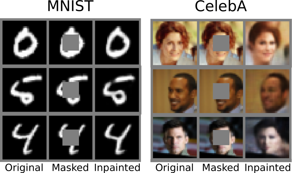
Figure 5: Inpainted images obtained using the generator $f_{\theta}$ trained with PGD as described in the text.

We use generators $f_{\theta_{K}}$ trained with PGD, ABP, SR, and VAE to recover images $y=(y_{i})_{i=1}^{d_{y}}$ that have been corrupted by masking some of their pixels. To do so, we follow the approach taken in Nijkamp et al. (2020, Sec. 5.3): we search for latent variables that maximize the likelihood of the corrupted image $y_{c}$,

$$x_{\text{mle}}=\textrm{argmax}_{x\in\mathbb{R}^{dx}}\log p(y_{c}|x)=\textrm{argmin}_{x\in\mathbb{R}^{dx}}\|y_{c}-f_{\theta_{K}}(x)\|^{2}_{2}=\textrm{argmin}_{x\in\mathbb{R}^{dx}}\sum_{i\not\in\mathcal{M}}[y_{i}-f_{\theta_{K}}(x)_{i}]^{2},$$ (73)

where $\mathcal{M}$ indexes the masked pixels. Then, we recover the image by mapping $x_{\text{mle}}$ through the generator: $y\approx f_{\theta}(x_{\textrm{mle}})$. To (approximately) solve the above we use $4$ randomly initialized runs of Adam (Kingma and Ba, 2014), each a thousand steps long. We set the learning rate adaptively using Pytorch’s ReduceLROnPlateau scheduler with an initial learning rate of $1$ and all other Adam parameters set to their Pytorch 1.12 defaults. With this approach, and the PGD-trained generator, we obtained the inpaintings shown in Fig. 5.

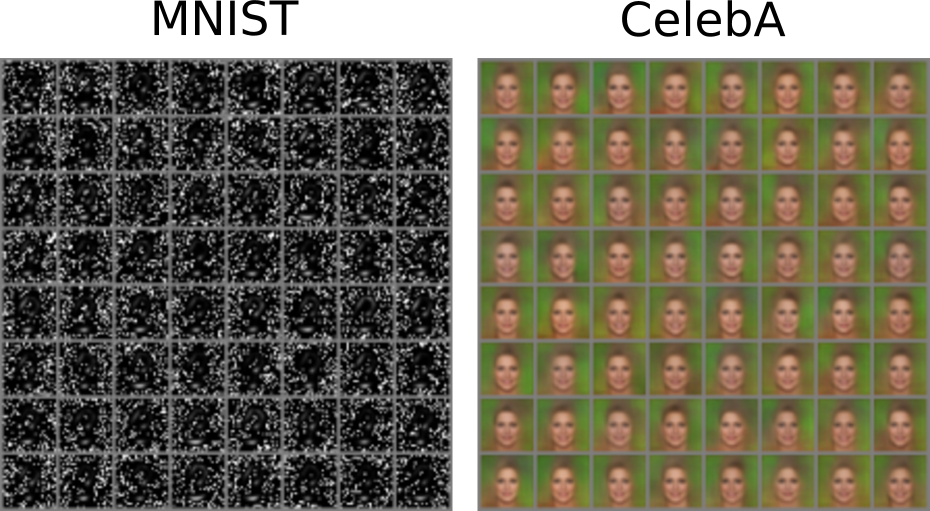
Figure 6: Images synthesized by drawing samples from the Gaussian prior $p(x)$ and mapping them through the generator $f_{\theta_{K}}$ trained with PGD.

Image synthesis.

Regardless of the algorithm we used for training, synthesizing images following the usual approach of drawing latent variables $x$ from the prior $p(x)$ and mapping them through the trained generator $f_{\theta_{K}}$ gave poor results (e.g. Fig. 6). This is a known issue for these types of models. For example, as explained in Aneja et al. (2021):

“Variational autoencoders (VAEs) are one of the powerful likelihood-based generative models with applications in many domains. However, they struggle to generate high-quality images, especially when samples are obtained from the prior without any tempering. One explanation for VAEs’ poor generative quality is the prior hole problem: the prior distribution fails to match the aggregate approximate posterior. Due to this mismatch, there exist areas in the latent space with high density under the prior that do not correspond to any encoded image. Samples from those areas are decoded to corrupted images.”

More specifically, in all four algorithms, we approximate the posterior $p_{\theta_{k}}(x^{1:M}|y^{1:M})$ using a product-form distribution:

$$q_{k}(dx^{1:M})=\prod_{m=1}^{M}q_{k}^{m}(dx^{m});$$

where $q_{k}^{m}(dx):=N^{-1}\sum_{n=1}^{N}\delta_{X^{n,m}_{k}}(dx)$ for PGD, $q_{k}^{m}(dx):=\delta_{X^{N,m}_{k}}(dx)$ for ABP and SR, and $q_{k}^{m}(dx):=q_{\phi_{k}}(dx|y^{m})$ for VAE. Emulating the calculations in Hoffman and Johnson (2016), we find that

$$F(\theta_{k},q_{k})=\sum_{m=1}^{M}\int\log\left(\frac{q_{k}^{m}(x^{m})}{p(x^{m})p_{\theta_{k}}(y^{m}|x^{m})}\right)q^{m}(x^{m})dx^{m}\geq\sum_{m=1}^{M}KL(q^{m}_{k}||p)\geq MKL(q^{agg}_{k}||p),$$ (74)

where

$$q^{agg}_{k}(dx):=\frac{1}{M}\sum_{m=1}^{M}q^{m}(dx)$$

denotes the aggregate (approximate) posterior (Aneja et al., 2021). To derive the rightmost inequality in (74) note that

$$\sum_{m=1}^{M}KL(q^{m}_{k}||p)-MKL(q^{agg}_{k}||p)=\sum_{m=1}^{M}\int\log\left(\frac{q^{m}_{k}(x)}{q^{agg}_{k}(x)}\right)q^{m}_{k}(x)dx$$

$$\qquad\qquad=\sum_{m=1}^{M}\int\log\left(\frac{q^{m}_{k}(x)}{Mq^{agg}_{k}(x)}\right)q^{m}_{k}(x)dx+M\log(M)$$

$$\qquad\qquad=M\int\left[\sum_{m=1}^{M}\log\left(\frac{q^{m}_{k}(x)}{Mq^{agg}_{k}(x)}\right)\frac{q^{m}_{k}(x)}{Mq^{agg}_{k}(x)}\right]q^{agg}_{k}(x)dx+Mlog(M)$$

For each $x$, the term inside the square brackets is the negative entropy of the distribution $\left(\frac{q^{m}_{k}(x)}{Mq^{agg}_{k}(x)}\right)_{m=1}^{M}$ and, hence, bounded below by $-\log(M)$; and (74) follows.

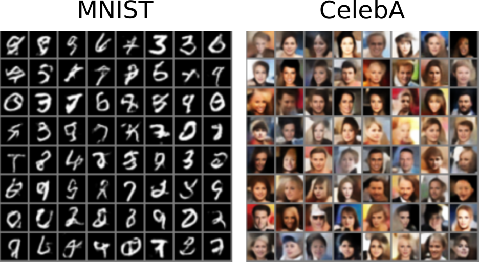
Figure 7: Images synthesized by sampling a Gaussian approximation of the PGD aggregate posterior.

(74) shows that the free energy is bounded below by $M$ times the KL divergence between the aggregate posterior $q_{k}^{agg}$ and the prior $p$. As noted in (Rosca et al., 2018):

“VAEs are unable to match the marginal latent posterior (aggregate posterior) to the prior. This will result in a failure to learn the data distribution, and manifests in a discrepancy in quality between samples and reconstructions from the model.”

In our experiments, we observed the same phenomenon for PGD, ABP, SR, and VAE. In all four cases, it appears that the model learns to generate qualitatively meaningful images in the regions of the latent space where the aggregate posterior places mass but not in those where the prior does.

To overcome the bottleneck in (74) and improve the image generation, a variety of schemes that learn the prior as well as the generator $f_{\theta}$ have been proposed in the literature (e.g. Tomczak and Welling (2018); Bauer and Mnih (2019); Klushyn et al. (2019); Dai and Wipf (2019); Pang et al. (2020); Aneja et al. (2021)). We limit ourselves to simply fitting a Gaussian $\mathcal{N}(\mu,\Sigma)$ to the (trained) aggregate posterior $q_{K}^{agg}$. For PGD, ABP, and SR, $q_{K}^{agg}$ is an empirical distribution of the form $J^{-1}\sum_{j=1}^{J}\delta_{Z^{j}}$ and we fit $\mathcal{N}(\mu,\Sigma)$ using $q_{K}^{agg}$’s empirical mean and covariance:

$$\mu:=\frac{1}{J}\sum_{j=1}^{J}Z^{j},\quad\Sigma:=\frac{1}{J-1}\sum_{j=1}^{J}(Z^{j}-\mu)(Z^{j}-\mu)^{T}.$$

In the case of VAE, we first build an empirical distribution $J^{-1}\sum_{j=1}^{J}\delta_{Z^{j}}$ by drawing $10$ samples from each $q^{1}_{k},\dots,q^{M}_{k}$, and then proceed as above. Synthesizing images by drawing samples from $\mathcal{N}(\mu,\Sigma)$ and mapping them through $f_{\theta}$ then produces substantially higher quality images (Fig. 7). Building more refined approximations of the aggregate posterior further improves the images (Fig. 8).

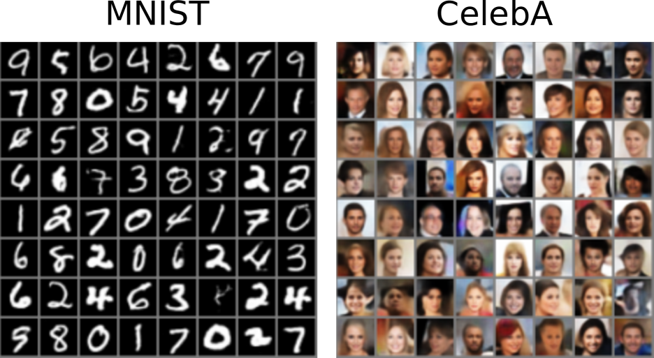
Figure 8: Images synthesized using by sampling a $500$-component mixture of Gaussian approximation of the PGD aggregate posterior. To fit the mixture, we applied scikit-learn’s default procedure to $J^{-1}\sum_{j=1}^{J}\delta_{Z^{j}}$.

Performance metrics.

To evaluate the performance the trained generators $f_{\theta_{K}}$ in the inpainting task, we mask and inpaint $1000$ images $y^{1},\dots,y^{1000}$ randomly chosen from the test set. For each of these, we solve (73) to obtain matching latent variable vectors $x^{1},\dots,x^{1000}$ and inpainted images $f_{\theta}(x^{1}),\dots,f_{\theta}(x^{1000})$. We then compute the latter’s mean squared error (averaged over both pixels and test images):

$$MSE=\frac{1}{1000d_{y}}\sum_{m=1}^{1000}\sum_{i=1}^{d_{y}}[y^{m}_{i}-f_{\theta}(x^{m})_{i}]^{2}.$$

To evaluate the performance of the trained generators $f_{\theta_{K}}$ in the synthesis task, we synthesize $200$ images as described above, randomly pick $200$ images from the test set, and compute the corresponding Fréchet Inception Distance (FID; Heusel et al. (2017)) with the Inception v3 classifier (Szegedy et al., 2016) between these two ensembles — we use TorchMetrics’s (Detlefsen et al., 2022) implementation of FID. In the case of the greyscale MNIST images, this requires mirroring the image across the three colour channels. We recognize that there are conceptual difficulties with this ad hoc approach, especially given that the training data for Inception v3 differs qualitatively from the MNIST images. However, we verified that there is a qualitative (as judged by eye) improvement in image quality associated with increasing FID score computed in this way and felt it sensible to follow this now-established approach for this dataset (e.g. see the papers reporting FID scores for MNIST on paperswithcode.com).

Appendix F THE MEAN-FIELD LIMITS AND THE TIME-DISCRETIZATION BIAS

The mean-field ($N\to\infty$) limits of PGD’s update equations, (14,15), are (75,76), those of PQN’s, (33,15), are (77,76), and that of PMGD’s, (44), is (78):

$$\theta_{k+1} =\theta_{k}+h\int\nabla_{\theta}\ell(\theta_{k},x)q_{k}(x)dx,$$ (75)

$$X_{k+1} =X_{k}+h\nabla_{x}\ell(\theta_{k},X_{k})+\sqrt{2h}W_{k},$$ (76)

$$\theta_{k+1} =\theta_{k}-h\left[\nabla_{\theta}^{2}\ell(\theta,x)q_{k}(x)dx\right]^{-1}\int\nabla_{\theta}\ell(\theta_{k},x)q_{k}(x)dx,$$ (77)

$$X_{k+1} =X_{k}+h\nabla_{x}\ell(\theta_{*}(q_{k}),X_{k})+\sqrt{2h}W_{k}.$$ (78)

where, in all cases, $q_{k}$ denotes $X_{k}$’s law and, in (78) we are assuming that Assumpt. 2 holds. We can re-write (75,77) as

$$\theta_{k+1}=u(\theta_{k},q_{k}),$$ (79)

where $u:\Theta\times\mathcal{P}(\mathcal{X})\to\Theta$ denotes an ‘update’ operator satisfying

$$\forall(\theta,q)\in\Theta\times\mathcal{P}(\mathcal{X}),\quad\nabla_{\theta}F(\theta,q)=0\enskip\Rightarrow\enskip u(\theta,q)=\theta.$$ (80)

Now, (76,79)’s joint law $q_{k}(d\theta,dx)$ satisfies

$$q_{k+1}(d\psi,dz)=\int_{\theta,x}q_{k}(d\theta,dx)\delta_{u(\theta,q_{k})}(d\psi)K_{\theta}(x,dz),$$ (81)

where $K_{\theta}$ denotes the ULA kernel:

$$K_{\theta}(x,dz)=K_{\theta}(x,z)dz:=\mathcal{N}\left(z;x+h\nabla_{x}\ell(\theta,x),2hI_{D_{x}}\right)dz\quad\forall x\in\mathcal{X},\enskip\theta\in\Theta.$$ (82)

What we would like is for

$$\pi(d\theta,dx):=\delta_{\theta_{*}}(d\theta)p_{\theta_{*}}(dx|y)$$

to be a fixed point of (81) whenever $\theta_{*}$ is a maximizer of $\theta\mapsto p_{\theta}(y)$ and $p_{\theta_{*}}(dx|y)$ is the corresponding posterior. However, applying Thrm. 2 and (80), we find that

$$\int_{\theta,x}\pi(d\theta,dx)\delta_{u(\theta,\pi(dx))}(d\psi)K_{\theta}(x,dz) =\int_{\theta,x}\delta_{\theta_{*}}(d\theta)p_{\theta_{*}}(dx|y)\delta_{u(\theta,p_{\theta_{*}}(dx|y))}(d\psi)K_{\theta}(x,dz)$$

$$=\delta_{u(\theta_{*},p_{\theta_{*}}(dx|y))}(d\psi)\int_{x}p_{\theta_{*}}(dx|y)K_{\theta_{*}}(x,dz)$$

$$=\delta_{\theta_{*}}(d\psi)\int_{x}p_{\theta_{*}}(dx|y)K_{\theta_{*}}(x,dz).$$

Hence, $\pi$ is a fixed point of (81) if and only $p_{\theta_{*}}(dx|y)$ is a stationary distribution of $K_{\theta_{*}}(x,dz)$:

$$p_{\theta_{*}}(z|y)=\int p_{\theta_{*}}(x|y)K_{\theta_{*}}(x,z)dx$$ (83)

However, we know this is not the case because the ULA kernel is biased, e.g. see Roberts and Tweedie (1996).

The case of (78) is similar: $q_{k}$ satisfies

$$q_{k+1}(z)=\int q_{k}(x)K_{\theta_{*}(q_{k})}(x,z)dx.$$

Given that $\theta_{*}(p_{\theta_{*}}(\cdot|y))=\theta_{*}$ (Thrm. 2), we have that $p_{\theta_{*}}(\cdot|y)$ is a fixed point of the above if and only if (83) holds, which it does not.

An obvious way to get (83) to hold is replacing the ULA kernel $K_{\theta}$ with a kernel whose stationary distribution is the posterior $p_{\theta}(\cdot|y)$ (e.g. by adding an accept-reject step to the ULA kernel). This removes the time-discretization bias in the mean-field regime. In App. H, we will see another (slightly less obvious) way to do so.

F.1 Rates of convergence for Ex. 1

To investigate the rate of convergence of PGD, PQN, and PMGD in the case of the toy hierarchical model (Ex. 1), we examine the mean-field limits (75–78) which respectively read:

$$\theta_{k+1} =\theta_{k}+hD_{x}[\nu_{k}-\theta_{k}],$$ (84)

$$X_{k+1} =X_{k}+h[y+\theta_{k}\bm{1}_{D_{x}}-2X_{k}]+\sqrt{2h}W_{k},$$ (85)

$$\theta_{k+1} =\theta_{k}+h\left[\nu_{k}-\theta_{k}\right],$$ (86)

$$X_{k+1} =X_{k}+h\left[y+\nu_{k}\bm{1}_{D_{x}}-2X_{k}\right]+\sqrt{2h}W_{k}.$$ (87)

where, in all cases, $\nu_{k}:=\mathbb{E}\left[\bm{1}_{D_{x}}^{T}X_{k}/D_{x}\right]$ denotes the mean of the average of $X_{k}$’s components. Left-multiplying (85,87) by $D_{x}^{-1}\bm{1}_{D_{x}}^{T}$ and taking expectations in, we respectively find that

$$\nu_{k+1} =\nu_{k}+h[\bm{1}_{D_{x}}^{T}y/D_{x}+\theta_{k}-2\nu_{k}]$$ (88)

$$\nu_{k+1} =\nu_{k}+h\left[\bm{1}_{D_{x}}^{T}y/D_{x}-\nu_{k}\right].$$ (89)

Note that both (84,88) and (86,88) have a unique fixed point $(\theta_{\infty},\nu_{\infty})$ given by $\theta_{\infty}=\nu_{\infty}=\theta_{*}$, where $\theta_{*}=\bm{1}_{D_{x}}^{T}y/D_{x}$ denotes the marginal likelihood’s unique maximizer (cf. App. E.1). Re-writing (84,88) and (86,88) in matrix-vector notation,

$$\begin{bmatrix}\theta_{k+1}\\ \nu_{k+1}\end{bmatrix} =A_{h}^{G}\begin{bmatrix}\theta_{k}\\ \nu_{k}\end{bmatrix}+\begin{bmatrix}0\\ h\bm{1}_{D_{x}}^{T}y/D_{x}\end{bmatrix}\quad\text{where}\quad A_{h}^{G}:=\begin{bmatrix}1-hD_{x}&hD_{x}\\ h&1-2h\end{bmatrix},$$

$$\begin{bmatrix}\theta_{k+1}\\ \nu_{k+1}\end{bmatrix} =A_{h}^{N}\begin{bmatrix}\theta_{k}\\ \nu_{k}\end{bmatrix}+\begin{bmatrix}0\\ h\bm{1}_{D_{x}}^{T}y/D_{x}\end{bmatrix}\quad\text{where}\quad A_{h}^{N}:=\begin{bmatrix}1-h&h\\ h&1-2h\end{bmatrix},$$

then clarifies that $\theta_{k}$’s speed of convergence to $\theta_{*}$ is $\mathcal{O}(\rho_{G,h}^{k})$ in the case of (84,88) and $\mathcal{O}(\rho_{N,h}^{k})$ in that of (86,88), where $\rho_{G,h}$ denotes $A_{h}^{G}$’s spectral radius and $\rho_{N,h}$ denotes $A_{h}^{N}$’s. After some quick algebra, we find that

$$\rho_{G,h}=\max\left\{\left|1-h\left(1+\frac{D_{x}}{2}\pm\frac{\sqrt{D^{2}_{x}+4}}{2}\right)\right|\right\},\quad\rho_{N,h}=\max\left\{\left|1-h\left(\frac{3}{2}\pm\frac{\sqrt{5}}{2}\right)\right|\right\}.$$

As for PMGD’s mean-field limit (87), recall that we use $\theta_{*}(q_{k})=D_{x}^{-1}\bm{1}^{T}_{D_{x}}\int xq_{k}(x)dx=\nu_{k}$ to estimate $\theta_{*}$, where $q_{k}$ denotes $X_{k}$’s law, and note that $\nu_{k}$ in (89) converges to $\theta_{*}$ at a rate of $\mathcal{O}(\rho_{M,h}^{k})$, where $\rho_{M,h}:=\left|1-h\right|$. Two observations are in order:

• Dependence on $D_{x}$. In the case of PGD, the radius $\rho_{G,h}$ depends on the dimension $D_{x}$ of the latent space. For large dimensions, $\rho_{G,h}\approx\left|1-h(1+D_{x})\right|$ implying that PGD is stable only for very small step sizes (roughly, those smaller than $2/(1+D_{x})$), which explains the need for the tweak (16). On the other hand, the radii for PQN and PMGD are independent of $D_{x}$. For these reasons, tuning the step size for PGD proves challenging and delicately depends on $D_{x}$, while tuning it for PQN and PMGD is straightforward and does not require taking $D_{x}$ into account.

• Relative speeds. For all step sizes, $\rho_{G,h}$ and $\rho_{N,h}$ are both bounded below by $\rho_{M,h}$ (see Fig. 9), implying that PMGD always converges faster than PGD and PQN, at least in the mean-field regime. It is not necessarily the case that $\rho_{N,h}\leq\rho_{G,h}$: for small step sizes, this fails to hold. However, the range of $h$s for which $\rho_{N,h}>\rho_{G,h}$ decreases precipitously with the latent space dimension $D_{x}$ (Fig. 9). Hence, we expect PQN to outperform PGD unless we use very small step sizes (likely, those too small to achieve any reasonable convergence speed).

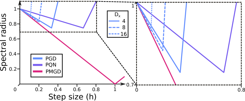
Figure 9: Spectral radii $\rho_{G,h}$ (PGD), $\rho_{N,h}$ (PQN), and $\rho_{M,h}$ (PMGD) as a function of step size $h$.

Consider now the matter of choosing the step size $h$ that achieves the fastest convergence for each algorithm. That is, the $h$ that minimizes the corresponding radius. It is straightforward to verify that

$$h_{G}=\frac{2}{2+D_{x}},\enskip h_{N}=\frac{2}{3},\enskip h_{M}=1,\quad\text{with}\quad\rho_{G}=\frac{\sqrt{D_{x}^{2}+4}}{D_{x}+2},\enskip\rho_{N}=\frac{\sqrt{5}}{3},\enskip\rho_{M}=0,$$

where $h_{G},h_{N},h_{M}$ respectively denote the optimal step sizes for PGD, PQN, and PMGD, and $\rho_{G},\rho_{N},\rho_{M}$ the corresponding radii. Note that, $\rho_{G}\geq\rho_{N}\geq\rho_{M}$ whenever $D_{x}\geq 4$. Hence, except for very low dimensional cases with well-tuned step sizes, PQN will outperform PGD. PMGD will always outperform either. Moreover, $\rho_{G}\to 1$ as $D_{x}\to\infty$ and, hence, PGD’s convergence speed degenerates with increasing latent space dimension regardless of the step size $h$ that we use. That of PQN does not and, if we tune the algorithm well, will be $\mathcal{O}([2/3]^{k})$ for all $D_{x}$. Setting $h:=1$ in (89), we find that, regardless of $D_{x}$, PMGD’s parameter estimates will converge in a single step, at least in the mean-field regime. Of course, this fails to materialize when we run the algorithm in practice because the noise in (87) exacts an $\mathcal{O}(1/\sqrt{KND_{x}})$ error in our time-averaged estimates, which is what we see in Fig. 1c (similar considerations also apply to PGD and PQN in stationarity). Lastly, we ought to mention that we have observed these behaviours replicated across other numerical experiments, hinting that they might hold more widely. However, until an analysis establishing so becomes available, we only count this as anecdotal evidence.

Appendix G THE CONTINUUM LIMITS AND THE FINITE-POPULATION-SIZE BIAS

For the sake of simplicity, suppose that Assumpt. 2 holds. The continuum limits ($h\to 0$) of PGD’s update equations, (14,15), are (90,91), those of PQN’s, (33,15), are (92,91), and that of PMGD’s, (44), is (93):

$$d\theta_{t} =\frac{1}{N}\left[\sum_{n=1}^{N}\nabla_{\theta}\ell(\theta_{t},X_{t}^{n})\right]dt,$$ (90)

$$dX_{t}^{n} =\nabla_{x}\ell(\theta_{t},X_{t}^{n})dt+\sqrt{2}dW_{t}^{n}\quad\forall n\in[N],$$ (91)

$$d\theta_{t} =-\left[\sum_{n=1}^{N}\nabla_{\theta}^{2}\ell(\theta_{t},X_{t}^{n})\right]^{-1}\left[\sum_{n=1}^{N}\nabla_{\theta}\ell(\theta_{t},X_{t}^{n})\right]dt,$$ (92)

$$dX_{t}^{n} =\nabla_{x}\ell(\theta_{*}(X_{t}^{1:N}),X_{t}^{n})dt+\sqrt{2}dW_{t}^{n}\quad\forall n\in[N].$$ (93)

As shown below, (93)’s law satisfies

$$\dot{q}_{t}(x^{1:N})=\nabla_{x^{1:N}}\cdot\left[q_{t}(x^{1:N})\nabla_{x^{1:N}}\log\left(\frac{q_{t}(x^{1:N})}{\rho_{N}(x^{1:N})}\right)\right],$$ (94)

where $\rho_{N}$ is the (unnormalized) distribution on $\mathcal{X}^{N}$ given by

$$\rho_{N}(x^{1:N}):=\prod_{n=1}^{N}p_{\theta_{*}(x^{1:N})}(x^{n},y)$$ (95)

Clearly, the (unique) normalized fixed point of (94) (i.e. the stationary distribution of (93)) is

$$\pi_{N}(x^{1:N}):=\frac{\rho_{N}(x^{1:N})}{\mathcal{Z}_{N}}\quad\text{where}\quad\mathcal{Z}_{N}:=\int\rho_{N}(x^{1:N})dx^{1:N}.$$ (96)

As also shown below, (90,91)’s law satisfies

$$\dot{q}_{t}(\theta,x^{1:N})= \nabla_{x^{1:N}}\cdot\left[q_{t}(\theta,x^{1:N})\nabla_{x^{1:N}}\log\left(\frac{q_{t}(\theta,x^{1:N})}{\prod_{n=1}^{N}p_{\theta}(x^{n},y)}\right)\right]$$ (97)

$$-\nabla_{\theta}\cdot\left[\frac{q_{t}(\theta,x^{1:N})}{N}\sum_{n=1}^{N}\nabla_{\theta}\ell(\theta,x^{n})\right],$$

where, if necessary, the above should be interpreted weakly. Because $\sum_{n=1}^{N}\nabla_{\theta}\ell(\theta_{*}(x^{1:N}),x^{n})=0$ by $\theta_{*}(x^{1:N})$’s definition, it is easy to check that

$$\pi_{N}(d\theta,dx^{1:N})=\delta_{\theta_{*}(x^{1:N})}(d\theta)\pi_{N}(x^{1:N})dx^{1:N}$$

is a fixed point of (97) (i.e. a stationary distribution of (90,91)). Similar manipulations show that the above is also a stationary distribution of (91,92). Our algorithms use the empirical distribution of the particles to approximate the posterior. Hence, for the estimates they produce to be ‘unbiased’, it would have to be the case that

$$\int\left(\theta_{*}(x^{1:N}),\frac{1}{N}\sum_{n=1}^{N}\delta_{x^{n}}(dx)\right)\pi_{N}(dx^{1:N})=(\theta_{*},p_{\theta_{*}}(dx|y)),$$

for some stationary point $\theta_{*}$ of $\theta\mapsto p_{\theta}(y)$. However, because $\theta_{*}(x^{1:N})$ is invariant to permutations of $x^{1:N}$’s components, $\pi_{N}$’s definition in (95,96) implies that its marginals $\pi_{N}(dx^{1}),\dots,\pi_{N}(dx^{N})$ all equal the same distribution, $\mu_{N}$ on $\mathcal{X}$. Hence,

$$\int\left(\frac{1}{N}\sum_{n=1}^{N}\delta_{x^{n}}(dx)\right)\pi_{N}(dx^{1:N}) =\frac{1}{N}\sum_{n=1}^{N}\int\delta_{x^{n}}(dx)\pi_{N}(dx^{n})=\frac{1}{N}\sum_{n=1}^{N}\int\delta_{x^{n}}(dx)\mu_{N}(dx^{n})$$

$$=\frac{1}{N}\sum_{n=1}^{N}\int\mu_{N}(dx)=\mu_{N}(dx).$$

In summary, for our algorithms to yield unbiased estimates, it would need to be the case that

$$\left(\int\theta_{*}(x^{1:N})\pi_{N}(dx^{1:N}),\mu_{N}(dx)\right)=(\theta_{*},p_{\theta_{*}}(dx|y)).$$

It is easy to find examples in which the above fails to hold (see, for instance, App. G.1).

Proof of (94).

(93)’s Fokker-Planck equation (e.g. see Chaintron and Diez (2022)) reads

$$\dot{q}_{t}(x^{1:N})= -\sum_{n=1}^{N}\nabla_{x^{n}}\cdot[q_{t}(x^{1:N})\nabla_{x^{n}}\ell(\theta_{*}(x^{1:N}),x^{n})]+\sum_{n=1}^{N}\nabla_{x^{n}}\cdot\nabla_{x^{n}}q_{t}(x^{1:N}).$$ (98)

But

$$-\nabla_{x^{1:N}}\cdot\left[q_{t}(x^{1:N})\nabla_{x^{1:N}}\log\left(\frac{\rho_{N}(x^{1:N})}{q_{t}(x^{1:N})}\right)\right]=-\sum_{n=1}^{N}\nabla_{x^{n}}\cdot\left[q_{t}(x^{1:N})\nabla_{x^{n}}\log\left(\frac{\rho_{N}(x^{1:N})}{q_{t}(x^{1:N})}\right)\right],$$ (99)

and, using $\rho_{N}(x^{1:N})$’s definition in (95),

$$\nabla_{x^{n}}\log\left(\frac{\rho_{N}(x^{1:N})}{q_{t}(x^{1:N})}\right)= \nabla_{x^{n}}\log(\rho_{N}(x^{1:N}))-\nabla_{x^{n}}\log(q_{t}(x^{1:N}))$$

$$= \nabla_{x^{n}}\ell(\theta_{*}(x^{1:N}),x^{n})+\sum_{m=1}^{N}\nabla_{\theta}\ell(\theta_{*}(x^{1:N}),x^{m})\cdot\nabla_{x^{m}}\theta_{*}(x^{1:N})$$

$$-\frac{\nabla_{x^{n}}q_{t}(x^{1:N})}{q_{t}(x^{1:N})}.$$ (100)

But, $\theta_{*}(x^{1:N})$’s definition implies that

$$\nabla_{x^{1}}\theta_{*}(x^{1:N})=\dots=\nabla_{x^{N}}\theta_{*}(x^{1:N}),\qquad\sum_{m=1}^{N}\nabla_{\theta}\ell(\theta_{*}(x^{1:N}),x^{m})=0.$$

Hence, the middle term in (100)’s RHS equals zero and (94) follows from (98,99). ∎

Proof of (97).

This is straightforward: (90,91)’s Fokker-Planck equation (e.g. see Chaintron and Diez (2022)) reads

$$\dot{q}_{t}(\theta,x^{1:N})= -\nabla_{\theta}\cdot\left[\frac{q_{t}(\theta,x^{1:N})}{N}\sum_{n=1}^{N}\nabla_{\theta}\ell(\theta,x^{n})\right]-\sum_{n=1}^{N}\nabla_{x^{n}}\cdot[q_{t}(\theta,x^{1:N})\nabla_{x^{n}}\ell(\theta,x^{n})]$$

$$+\sum_{n=1}^{N}\nabla_{x^{n}}\cdot\nabla_{x^{n}}q_{t}(\theta,x^{1:N}).$$

But,

$$\nabla_{x^{1:N}}\cdot\left[q_{t}(\theta,x^{1:N})\nabla_{x^{1:N}}\log\left(\frac{\prod_{n=1}^{N}p_{\theta}(x^{n},y)}{q_{t}(\theta,x^{1:N})}\right)\right]$$

$$=\sum_{n=1}^{N}\nabla_{x^{n}}\cdot\left[q_{t}(\theta,x^{1:N})\nabla_{x^{n}}\log\left(\frac{\prod_{n=1}^{N}p_{\theta}(x^{n},y)}{q_{t}(\theta,x^{1:N})}\right)\right]$$

$$=\sum_{n=1}^{N}\nabla_{x^{n}}\cdot\left[q_{t}(\theta,x^{1:N})\left(\nabla_{x^{n}}\ell(\theta,x^{n})-\frac{\nabla_{x^{n}}q_{t}(\theta,x^{1:N})}{q_{t}(\theta,x^{1:N})}\right)\right]$$

$$=\sum_{n=1}^{N}\nabla_{x^{n}}\cdot[q_{t}(\theta,x^{1:N})\nabla_{x^{n}}\ell(\theta,x^{n})]+\sum_{n=1}^{N}\nabla_{x^{n}}\cdot\nabla_{x^{n}}q_{t}(\theta,x^{1:N}).$$

∎

G.1 Continuum limits for Ex. 1

By (54) and $\rho_{N}$’s definition in (95),

$$\rho_{N}(x^{1:N}) =\prod_{n=1}^{N}\exp\left(-\frac{1}{2}\left|\left|{y-x^{n}}\right|\right|^{2}-\frac{1}{2}\left|\left|{x^{n}-\frac{\bm{1}^{T}_{ND_{x}}x^{1:N}}{ND_{x}}\bm{1}_{D_{x}}}\right|\right|^{2}\right)$$

$$=\exp\left(-\frac{1}{2}\left|\left|{y^{1:N}-x^{1:N}}\right|\right|^{2}-\frac{1}{2}\left|\left|{x^{1:N}-\frac{\bm{1}^{T}_{ND_{x}}x^{1:N}}{ND_{x}}\bm{1}_{ND_{x}}}\right|\right|^{2}\right),$$

where $y^{1:N}$ stacks $N$ copies of $y$. Applying the expressions in Bishop (2006, p. 92) and the Sherman–Morrison formula, we find that

$$\pi_{N}(x^{1:N})=\frac{\rho_{N}(x^{1:N})}{\int\rho_{N}(x^{1:N})dx^{1:N}}=\mathcal{N}\left(x^{1:N};\frac{1}{2}\left(y^{N}+\frac{\bm{1}^{T}_{D_{x}}y}{D_{x}}\bm{1}_{ND_{x}}\right),\frac{1}{2}\left(I_{ND_{x}}+\frac{\bm{1}_{ND_{x}}\bm{1}^{T}_{ND_{x}}}{ND_{x}}\right)\right);$$

whose marginals are equal to

$$\mu_{N}(x)=\mathcal{N}\left(x;\frac{1}{2}\left(y+\frac{\bm{1}^{T}_{D_{x}}y}{D_{x}}\bm{1}\right),\frac{1}{2}\left(I_{D_{x}}+\frac{\bm{1}_{D_{x}}\bm{1}^{T}_{D_{x}}}{ND_{x}}\right)\right).$$

Comparing with (51), we see that the covariance matrix is slightly off with a $\mathcal{O}(N^{-1})$ error. However, due to the linearity in the model, there is no bias in the $\theta$ estimates:

$$\int\theta_{*}(x^{1:N})\pi_{N}(x^{1:N})dx^{1:N} =\frac{\bm{1}^{T}_{ND_{x}}\int x^{1:N}\pi_{N}(x^{1:N})dx^{1:N}}{ND_{x}}$$

$$=\frac{1}{2ND_{x}}\left(\bm{1}^{T}_{ND_{x}}y^{N}+\frac{\bm{1}^{T}_{ND_{x}}\bm{1}_{ND_{x}}\bm{1}^{T}_{D_{x}}y}{D_{x}}\right)=\frac{\bm{1}^{T}_{D_{x}}y}{D_{x}}=\theta_{*}.$$

Appendix H METROPOLIS-HASTINGS METHODS

As mentioned at the end of App. F, one fairly obvious way to try to remove the bias (B1, Sec. 2) from the estimates produced by PGD, PQN, and PMGD is to replace the ULA kernels with ‘exact’ kernels whose stationary distributions coincide with the posteriors (e.g. by adding an accept-reject step to each individual particle update). Here, we consider other, slightly less obvious and (to the best of our knowledge) novel extensions of the Metropolis-Hastings algorithm (e.g. see Andrieu et al. (2003)) that also tackle (S1,2 in Sec. 1). While these methods need not necessarily be associated with an optimization routine, their comprehension is also aided by viewing (S1,2) as a joint problem over $\theta$ and $q$. The methods have one practical downside that limits their scalability: similar to standard Metropolis-Hastings algorithms (e.g. see Beskos et al. (2013); Vogrinc et al. (2022); Kuntz et al. (2019a, b) and references therein), the acceptance probability degenerates with increasing latent variable dimensions $D_{x}$ and the particle numbers $N$. This, in turn, forces us to choose small step sizes $h$ for large $D_{x}$ and $N$, which leads to slow convergence. This is why we focused on the ‘unadjusted’ methods in the main text rather than the Metropolized ones in this appendix.

H.1 Marginal variants

1:  Initial conditions: $X^{1:N}_{0}:=(X^{1}_{0},\dots,X_{0}^{N})$.

2:  for $k=0,\dots,K-1$ do

3:     Propose: draw $Z^{1:N}=(Z^{1},\dots,Z^{N})$ from $K_{N}$.

4:     Generate uniform R.V.: draw $U_{k}$ from the uniform distribution on $[0,1]$.

5:     if If $U_{k}\leq a(X^{1:N}_{k},Z^{1:N})$, with $a(\cdot,\cdot)$ as in (101) then

6:        Accept: set $X_{k+1}^{1:N}:=Z^{1:N}$.

7:     else

8:        Reject: set $X_{k+1}^{1:N}:=X_{k}^{1:N}$.

9:     end if

10:  end for

Algorithm 4 The marginal MH method.

Suppose that Assumpt. 2 holds and, for the sake of discussion, that the marginal likelihood $\theta\mapsto p_{\theta}(y)$ has a unique maximizer $\theta_{*}$. Notice that the entire particle system $(X_{k}^{1:N})_{k=0}^{\infty}:=(X_{k}^{1},\dots,X_{k}^{N})_{k=0}^{\infty}$ generated by PMGD (44) is a Markov chain taking values in $\mathcal{X}^{N}$. Its kernel is given by

$$K_{N}(x^{1:N},z^{1:N}):=\prod_{n=1}^{N}K_{\theta_{*}(x^{1:N})}(x^{n},z^{n}),$$

where $K_{\theta}$ denotes the ULA kernel in (82). (The precise form of $K_{\theta}$ is immaterial to the ensuing discussion as long as, for each $\theta$, $K_{\theta}$ is a Markov kernel on $\mathcal{X}$.) Ideally, $K_{N}$’s stationary distribution would be $\prod_{n=1}^{N}p_{\theta_{*}}(x^{n}|y)$ but (B1,2 in Sec. 2) preclude it. Correcting for this using an accept-reject step requires evaluating $\prod_{n=1}^{N}p_{\theta_{*}}(x^{n},y)$, which we cannot do because $\theta_{*}$ is unknown. We can, however, evaluate $\rho_{N}(x^{1:N})$ in (95) and instead add an accept-reject step with acceptance probability

$$a_{N}(x^{1:N},z^{1:N}):=1\wedge\left(\frac{\rho_{N}(z^{1:N})K_{N}(z^{1:N},x^{1:N})}{\rho_{N}(x^{1:N})K_{N}(x^{1:N},z^{1:N})}\right).$$ (101)

Running Alg. 4, we then obtain a chain $(X_{k}^{1:N})_{k=0}^{\infty}$ whose stationary distribution is given by $\rho_{N}(x^{1:N})$’s normalization, $\pi_{N}(x^{1:N})$ in (96). Under Assumpt. 2, $\pi_{N}(x^{1:N})$ is the unique fixed point of the continuum limits of PGD, PQN, and PMGD, see App. G. In other words, by imposing the accept-reject step, we have removed the (B1, Sec. 2) source of bias (see Fig. 2c).

The other source, (B2, Sec. 2) due to the finite population size, remains, but it can be mitigated by growing $N$. In particular, by its definition, $\theta_{*}(x^{1:N})$ is invariant to permutations $x^{1:N}$’s components. Hence, the components of any vector $(X^{1},\dots,X^{N})$ drawn from $\pi_{N}$ are exchangeable (similarly for $(X_{k}^{1},\dots,X_{k}^{N})$ in Alg. 4). By chaos (e.g. Chaintron and Diez (2022); Hauray and Mischler (2014)), we expect that, under appropriate technical conditions, there exists a distribution $\pi$ in $\mathcal{P}(\mathcal{X})$ to which all of $\pi_{N}$’s marginals converge. It should follow that, under $\pi_{N}$,

$$\frac{1}{N}\sum_{n=1}^{N}\delta_{x^{n}}\approx\pi\quad\Rightarrow\quad\theta_{*}(x^{1:N})=\theta_{*}\left(\frac{1}{N}\sum_{n=1}^{N}\delta_{x^{n}}\right)\approx\theta_{*}(\pi),$$

with the above holding exactly in the $N\to\infty$ limit. Marginalising (95,96) and taking limits we would then find that $\pi(x)\propto p_{\theta_{*}(\pi)}(x,y)$. In other words, $\pi$ satisfies the first order optimality condition for $F_{*}$ in Thrm. 5: $\nabla F_{*}(\pi)=0$. It then follows from $\theta_{*}(q)$’s definition and Thrm. 5, that $\theta_{*}(\pi)$ is a stationary point of $\theta\mapsto p_{\theta}(y)$ and $\pi$ is the corresponding posterior $p_{\theta_{*}(\pi)}(\cdot|y)$. While we yet lack rigorous statements formalizing this discussion, it is easy to verify that it holds true for analytically tractable models (e.g. App. G.1), and our numerical experiments seem to corroborate it further (e.g. Fig. 2c).

H.2 Joint variants

We can also mitigate (B1, Sec. 2) for PGD (Alg. 1) and PQN (Alg. 2) using a population-wide accept-reject step along the lines of that in App. H.1. To begin, note that these algorithms are special cases of

$$\theta_{k+1} =u(\theta_{k},q_{k}^{N})\quad\text{with}\quad q_{k}^{N}:=\frac{1}{N}\sum_{n=1}^{N}\delta_{X_{k}^{n}},$$ (102)

$$X_{k+1}^{1:N} \sim K_{N}^{\theta_{k}}(X_{k}^{1:N},\cdot)\quad\text{with}\quad K_{N}^{\theta}(x^{1:N},z^{1:N}):=\prod_{n=1}^{N}K_{\theta}(x^{n},z^{n}),$$ (103)

where $K_{\theta}$ denotes a Markov kernel on $\mathcal{X}$ for each $\theta$ in $\Theta$ (in particular, the ULA kernel in (82), but this is once again unimportant) and $u$ denotes an update operator satisfying (80). Clearly, $(\theta_{k},X_{k}^{1},\dots,X_{k}^{N})_{k=0}^{\infty}$ forms a Markov chain with transition kernel

$$K_{N}((\theta,x^{1:N}),(d\psi,dz^{1:N}))=\delta_{u\left(\theta,\bar{\delta}_{x^{1:N}}\right)}(d\psi)K_{N}^{\theta}(x^{1:N},dz^{1:N})\quad\text{where}\quad\bar{\delta}_{x^{1:N}}:=\frac{1}{N}\sum_{n=1}^{N}\delta_{x^{n}}.$$

Emulating our steps in App. H.1, we impose an accept-reject step with acceptance probability

$$a_{N}((x^{1:N},\theta),(z^{1:N},\psi)):=1\wedge\left(\frac{K^{\psi}_{N}(z^{1:N},x^{1:N})}{K^{\theta}_{N}(x^{1:N},z^{1:N})}\prod_{n=1}^{N}\frac{p_{\psi}(z^{n},y)}{p_{\theta}(x^{n},y)}\right),$$ (104)

so obtaining Alg. 5.

1:  Initial conditions: $\theta_{0}$ and $X^{1:N}_{0}:=(X^{1}_{0},\dots,X_{0}^{N})$.

2:  for $k=0,\dots,K-1$ do

3:     Propose: set $\psi:=u\left(\theta_{k},N^{-1}\sum_{n=1}^{N}\delta_{X_{k}^{n}}\right)$ and draw $Z^{1:N}$ from $K_{N}^{\theta_{k}}$.

4:     Generate uniform R.V.: draw $U_{k}$ independently from the uniform distribution on $[0,1]$.

5:     if $U_{k}\leq a((\theta_{k},X^{1:N}_{k},(\psi,Z^{1:N}))$, with $a(\cdot,\cdot)$ as in (104) then

6:        Accept: set $\theta_{k+1}:=\psi$ and $X_{k+1}^{1:N}:=Z^{1:N}$.

7:     else

8:        Reject: set $\theta_{k+1}:=\theta_{k}$ and $X_{k+1}^{1:N}:=X_{k}^{1:N}$.

9:     end if

10:  end for

Algorithm 5 The joint MH method.

We have so far failed to obtain analytical expressions for the resulting chain’s stationary distributions. However, it is straightforward to find heuristic arguments suggesting that, as $N\to\infty$, the $(\theta,x^{n})$-marginal, for any $n$, of these distributions approaches measures of the form $\delta_{\theta_{*}}(d\theta)p_{\theta_{*}}(x^{n}|y)dx^{n}$, where $\theta_{*}$ is a stationary point of the marginal likelihood. In particular, note that the i.i.d. structure in $K_{N}^{\theta}$’s definition ensures that the particle system is exchangeable (hence, $X_{k}^{1},\dots,X_{k}^{N}$ all have the same law $q_{k}$). By propagation of chaos (e.g. see Chaintron and Diez (2022)), it is reasonable to expect that, for large $N$, the particle’s empirical distribution, $q_{k}^{N}$ in (102), closely approximates $q_{k}$:

$$q_{k}^{N}\approx q_{k}.$$

Suppose that the above holds exactly, and consider the resulting ‘idealized version’ $(\tilde{\theta}_{k},\tilde{X}^{1:N}_{k})$ of the chain $(\theta_{k},X^{1:N}_{k})$ produced by Alg. 5: just as in (102,103), except that the empirical distribution $q_{k}^{N}$ in (102) is replaced by the exact law $q_{k}$. The idealized chain’s one-dimensional law $\mu_{k}(d\theta,dx^{1:N})$ satisfies

$$\mu_{k+1}(d\psi,dz^{1:N})=\int\mu_{k}(d\theta,dx^{1:N})P_{N}^{q_{k}}((\theta,x^{1:N}),(d\psi,dz^{1:N})),$$ (105)

where the ‘idealized kernel’ $P_{N}^{q}$ is given by

$$P_{N}^{q}((\theta,x^{1:N}),(d\psi,dz^{1:N}))= a_{N}((\theta,x^{1:N}),(\psi,z^{1:N}))\delta_{u(\theta,q)}(d\psi)K^{\theta}_{N}(x^{1:N},z^{1:N})dz^{1:N}$$

$$+[1-a((\theta,x^{1:N}),(\psi,z^{1:N}))]\delta_{\theta}(d\psi)\delta_{x^{1:N}}(dz^{1:N}).$$

It is then straightforward to show that, for any stationary point $\theta_{*}$ of the marginal likelihood,

$$\pi_{N}^{*}(d\theta,dx):=\delta_{\theta_{*}}(d\theta)\prod_{n=1}^{N}p_{\theta_{*}}(x^{n}|y)dx^{n}$$

is a stationary distribution of the idealized chain in the sense that

$$(\tilde{\theta}_{0},\tilde{X}^{1:N}_{0})\sim\pi_{N}^{*}\quad\Rightarrow\quad(\tilde{\theta}_{k},\tilde{X}^{1:N}_{k})\sim\pi_{N}^{*}\enskip\forall k=1,2,\dots$$ (106)

In particular, detailed balance holds: for any $(\theta,x^{1:N})\neq(\psi,z^{1:N})$ satisfying

$$\qquad\qquad K^{\psi}_{N}(z^{1:N},x^{1:N})\prod_{n=1}^{N}p_{\psi}(z^{n},y)\leq K^{\theta}_{N}(x^{1:N},z^{1:N})\prod_{n=1}^{N}p_{\theta}(x^{n},y),$$ (107)

$$\Rightarrow a_{N}((\theta,x^{1:N}),(\psi,z^{1:N}))=\frac{K^{\psi}_{N}(z^{1:N},x^{1:N})}{K^{\theta}_{N}(x^{1:N},z^{1:N})}\prod_{n=1}^{N}\frac{p_{\psi}(z^{n},y)}{p_{\theta}(x^{n},y)},\quad a_{N}((\psi,z^{1:N}),(\theta,x^{1:N}))=1,$$

we have that, with $\pi_{*}(\cdot):=p_{\theta_{*}}(\cdot|y)$,

$$\pi_{N}^{*}(d\theta,dx^{1:N})P^{\pi_{*}}_{N}((\theta,x^{1:N}),(d\psi,dz^{1:N}))$$

$$=\delta_{\theta_{*}}(d\theta)\left(\prod_{n=1}^{N}p_{\theta_{*}}(x^{n}|y)\right)a_{N}((\theta,x^{1:N}),(\psi,z^{1:N}))\delta_{u(\theta,\pi_{*})}(d\psi)K^{\theta}_{N}(x^{1:N},z^{1:N})dx^{1:N}dz^{1:N}$$

$$=\delta_{\theta_{*}}(d\theta)\left(\prod_{n=1}^{N}p_{\theta_{*}}(x^{n}|y)\frac{p_{\psi}(z^{n},y)}{p_{\theta}(x^{n},y)}\right)\delta_{u(\theta,\pi_{*})}(d\psi)K^{\psi}_{N}(z^{1:N},x^{1:N})dx^{1:N}dz^{1:N}$$

$$=\delta_{\theta_{*}}(d\theta)\left(\prod_{n=1}^{N}p_{\theta_{*}}(x^{n}|y)\frac{p_{\psi}(z^{n},y)}{p_{\theta_{*}}(x^{n},y)}\right)\delta_{u(\theta_{*},\pi_{*})}(d\psi)K^{\psi}_{N}(z^{1:N},x^{1:N})dx^{1:N}dz^{1:N}$$

$$=\delta_{u(\theta_{*},\pi_{*})}(d\theta)\left(\prod_{n=1}^{N}\frac{p_{\theta_{*}}(z^{n},y)}{p_{\theta_{*}}(y)}\right)\delta_{\theta_{*}}(d\psi)K^{\psi}_{N}(z^{1:N},x^{1:N})dx^{1:N}dz^{1:N}$$

$$=\delta_{u(\psi,\pi_{*})}(d\theta)\left(\prod_{n=1}^{N}p_{\theta_{*}}(z^{n}|y)\right)\delta_{\theta_{*}}(d\psi)K^{\psi}_{N}(z^{1:N},x^{1:N})dx^{1:N}dz^{1:N}$$

$$=\delta_{u(\psi,\pi_{*})}(d\theta)\left(\prod_{n=1}^{N}p_{\theta_{*}}(z^{n}|y)\right)a_{N}((\psi,z^{1:N}),(\theta,x^{1:N}))\delta_{\theta_{*}}(d\psi)K^{\psi}_{N}(z^{1:N},x^{1:N})dx^{1:N}dz^{1:N}z$$

$$=\pi_{N}^{*}(d\psi,dz^{1:N})P_{N}^{\pi_{*}}((\psi,z^{1:N}),(d\theta,dx^{1:N})).$$

Reversing the roles of $(\theta,x^{1:N})$ and $(\psi,z^{1:N})$, we find that the above also holds should the inequality (107) be reversed. Because it holds trivially if $(\theta,x^{1:N})=(\psi,z^{1:N})$, integrating both sides over $(\theta,x^{1:N})$, we find that

$$\int\pi_{N}^{*}(d\theta,dx^{1:N})P^{\pi_{*}}_{N}((\theta,x^{1:N}),(d\psi,dz^{1:N}))=\pi_{N}^{*}(d\psi,dz^{1:N});$$

and (106) follows from (105).

References

- Ahn and Chewi (2021) K. Ahn and S. Chewi. Efficient constrained sampling via the mirror-Langevin algorithm. In Advances in Neural Information Processing Systems, volume 34, pages 28405–28418, 2021. URL https://proceedings.neurips.cc/paper/2021/file/ef1e491a766ce3127556063d49bc2f98-Paper.pdf.
- Ambrosio et al. (2005) L. Ambrosio, N. Gigli, and G. Savaré. Gradient flows: in metric spaces and in the space of probability measures. Birkhäuser Basel, 2005. URL https://doi.org/10.1007/b137080.
- Andrieu et al. (2003) C. Andrieu, N. de Freitas, A. Doucet, and M. I. Jordan. An introduction to MCMC for machine learning. Machine Learning, 50:5–43, 2003. URL https://doi.org/10.1023/A:1020281327116.
- Aneja et al. (2021) J. Aneja, A. Schwing, J. Kautz, and A. Vahdat. A contrastive learning approach for training variational autoencoder priors. In Advances in Neural Information Processing Systems, volume 34, pages 480–493, 2021. URL https://proceedings.neurips.cc/paper/2021/file/0496604c1d80f66fbeb963c12e570a26-Paper.pdf.
- Arnold et al. (2001) A. Arnold, P. Markowich, G. Toscani, and A. Unterreiter. On convex Sobolev inequalities and the rate of convergence to equilibrium for fokker-planck type equations. Communications in Partial Differential Equations, 26(1-2):43–100, 2001. URL https://doi.org/10.1081/PDE-100002246.
- Bauer and Mnih (2019) M. Bauer and A. Mnih. Resampled priors for variational autoencoders. In Proceedings of the Twenty-Second International Conference on Artificial Intelligence and Statistics, pages 66–75, 2019. URL https://proceedings.mlr.press/v89/bauer19a.html.
- Bernton (2018) E. Bernton. Langevin Monte Carlo and JKO splitting. In Proceedings of the 31st Conference On Learning Theory, volume 75 of PMLR, pages 1777–1798, 2018. URL https://proceedings.mlr.press/v75/bernton18a.html.
- Beskos et al. (2013) A. Beskos, N. Pillai, G. Roberts, J.-M. Sanz-Serna, and A. Stuart. Optimal tuning of the hybrid Monte Carlo algorithm. Bernoulli, 19(5A):1501–1534, 2013. URL https://doi.org/10.3150/12-BEJ414.
- Bishop (2006) C. M. Bishop. Pattern Recognition and Machine Learning. Springer New York, 2006.
- Boumal (2022) N. Boumal. An introduction to optimization on smooth manifolds. To appear with Cambridge University Press, 2022. URL http://www.nicolasboumal.net/book.
- Boyd and Vandenberghe (2004) S. P. Boyd and L. Vandenberghe. Convex Optimization. Cambridge University Press, 2004. URL https://doi.org/10.1017/CBO9780511804441.
- Bradbury et al. (2018) J. Bradbury, R. Frostig, P. Hawkins, M. J. Johnson, C. Leary, D. Maclaurin, G. Necula, A. Paszke, J. VanderPlas, S. Wanderman-Milne, and Q. Zhang. JAX: composable transformations of Python+NumPy programs, 2018. URL http://github.com/google/jax.
- Brascamp and Lieb (1976) H. J. Brascamp and E. H. Lieb. On extensions of the Brunn-Minkowski and Prékopa-Leindler theorems, including inequalities for log concave functions, and with an application to the diffusion equation. Journal of Functional Analysis, 22(4):366–389, 1976. URL https://doi.org/10.1016/0022-1236(76)90004-5.
- Cai (2010) L. Cai. High-dimensional exploratory item factor analysis by a Metropolis-Hastings Robbins-Monro algorithm. Psychometrika, 75(1):33–57, 2010. URL https://doi.org/10.1007/s11336-009-9136-x.
- Caron and Doucet (2012) F. Caron and A. Doucet. Efficient bayesian inference for generalized bradley–terry models. Journal of Computational and Graphical Statistics, 21(1):174–196, 2012. URL https://doi.org/10.1080/10618600.2012.638220.
- Carrillo et al. (2020) J. A. Carrillo, R. S. Gvalani, and J. Wu. An invariance principle for gradient flows in the space of probability measures. arXiv preprint arXiv:2010.00424, 2020. URL https://doi.org/10.48550/ARXIV.2010.00424.
- Chaintron and Diez (2022) L.-P. Chaintron and A. Diez. Propagation of chaos: a review of models, methods and applications. I. Models and methods. arXiv preprint arXiv:2203.00446, 2022. URL https://doi.org/10.48550/ARXIV.2203.00446.
- Chen et al. (2018) C. Chen, R. Zhang, W. Wang, B. Li, and L. Chen. In Conference on Uncertainty in Artificial Intelligence (UAI), 2018. URL http://auai.org/uai2018/proceedings/papers/263.pdf.
- Cheng and Bartlett (2018) X. Cheng and P. Bartlett. Convergence of Langevin MCMC in KL-divergence. In Proceedings of Algorithmic Learning Theory, volume 83, pages 186–211, 2018. URL https://proceedings.mlr.press/v83/cheng18a.html.
- Cheng et al. (2018) X. Cheng, N. S. Chatterji, P. L. Bartlett, and M. I. Jordan. Underdamped Langevin MCMC: A non-asymptotic analysis. In Proceedings of the 31st Conference On Learning Theory, volume 75 of PMLR, pages 300–323, 2018. URL https://proceedings.mlr.press/v75/cheng18a.html.
- Chewi et al. (2020) S. Chewi, T. Le Gouic, C. Lu, T. Maunu, P. Rigollet, and A. Stromme. Exponential ergodicity of mirror-Langevin diffusions. In Advances in Neural Information Processing Systems, volume 33, pages 19573–19585. Curran Associates, Inc., 2020. URL https://proceedings.neurips.cc/paper/2020/file/e3251075554389fe91d17a794861d47b-Paper.pdf.
- Csiszár and Tusnády (1984) I. Csiszár and G. Tusnády. Information geonetry and alternating minimization procedures. Statistics and decisions, Supp. 1:205–237, 1984.
- Dai and Wipf (2019) B. Dai and D. Wipf. Diagnosing and enhancing vae models. arXiv preprint arXiv:1903.05789, 2019. URL https://doi.org/10.48550/ARXIV.1903.05789.
- Dalalyan (2017) A. S. Dalalyan. Theoretical guarantees for approximate sampling from smooth and log-concave densities. Journal of the Royal Statistical Society: Series B (Statistical Methodology), 79(3):651–676, 2017. URL https://doi.org/10.1111/rssb.12183.
- De Bortoli et al. (2020) V. De Bortoli, A. Durmus, M. Pereyra, and A. Fernandez Vidal. Maximum likelihood estimation of regularization parameters in high-dimensional inverse problems: An empirical Bayesian approach. part ii: Theoretical analysis. SIAM Journal on Imaging Sciences, 13(4):1990–2028, 2020. URL https://doi.org/10.1137/20M1339842.
- De Bortoli et al. (2021) V. De Bortoli, A. Durmus, M. Pereyra, and A. Fernandez Vidal. Efficient stochastic optimisation by unadjusted Langevin Monte Carlo. Statistics and Computing, 31, 2021. URL https://doi.org/10.1007/s11222-020-09986-y.
- Delyon et al. (1999) B. Delyon, M. Lavielle, and É. Moulines. Convergence of a stochastic approximation version of the EM algorithm. The Annals of Statistics, 27(1):94–128, 1999. URL http://www.jstor.org/stable/120120.
- Dempster et al. (1977) A. P. Dempster, N. M. Laird, and D. B. Rubin. Maximum likelihood from incomplete data via the EM algorithm. Journal of the Royal Statistical Society: Series B (Methodological), 39(1):1–22, 1977. URL https://doi.org/10.1111/j.2517-6161.1977.tb01600.x.
- Detlefsen et al. (2022) N. S. Detlefsen, J. Borovec, J. Schock, A. H. Jha, T. Koker, L. Di Liello, D. Stancl, C. Quan, M. Grechkin, and W. Falcon. Torchmetrics - measuring reproducibility in pytorch. Journal of Open Source Software, 7(70):4101, 2022. URL https://doi.org/10.21105/joss.04101.
- Doucet et al. (2002) A. Doucet, S. J. Godsill, and C. P. Robert. Marginal maximum a posteriori estimation using Markov chain Monte Carlo. Statistics and Computing, 12:77–84, 2002. URL https://doi.org/10.1023/A:1013172322619.
- Duncan et al. (2019) A. Duncan, N. Nuesken, and L. Szpruch. On the geometry of Stein variational gradient descent. arXiv preprint arXiv:1912.00894, 2019. URL https://doi.org/10.48550/ARXIV.1912.00894.
- Durmus and Moulines (2017) A. Durmus and É. Moulines. Nonasymptotic convergence analysis for the unadjusted Langevin algorithm. The Annals of Applied Probability, 27(3):1551–1587, 2017. URL https://doi.org/10.1214/16-AAP1238.
- Durmus and Moulines (2019) A. Durmus and É. Moulines. High-dimensional Bayesian inference via the unadjusted Langevin algorithm. Bernoulli, 25(4A):2854–2882, 2019. URL https://doi.org/10.3150/18-BEJ1073.
- Durmus et al. (2018) A. Durmus, É. Moulines, and M. Pereyra. Efficient Bayesian computation by proximal Markov chain Monte Carlo: When Langevin meets Moreau. SIAM Journal on Imaging Sciences, 11(1):473–506, 2018. URL https://doi.org/10.1137/16M1108340.
- Durmus et al. (2019) A. Durmus, S. Majewski, and B. Miasojedow. Analysis of Langevin Monte Carlo via convex optimization. Journal of Machine Learning Research, 20(73):1–46, 2019. URL http://jmlr.org/papers/v20/18-173.html.
- Ermak (1975) D. L. Ermak. A computer simulation of charged particles in solution. I. Technique and equilibrium properties. The Journal of Chemical Physics, 62(10):4189–4196, 1975. URL https://doi.org/10.1063/1.430300.
- Fernandez Vidal et al. (2020) A. Fernandez Vidal, V. De Bortoli, M. Pereyra, and A. Durmus. Maximum likelihood estimation of regularization parameters in high-dimensional inverse problems: An empirical Bayesian approach part i: Methodology and experiments. SIAM Journal on Imaging Sciences, 13(4):1945–1989, 2020. URL https://doi.org/10.1137/20M1339829.
- Garbuno-Inigo et al. (2020) A. Garbuno-Inigo, F. Hoffmann, W. Li, and A. M. Stuart. Interacting Langevin diffusions: Gradient structure and ensemble Kalman sampler. SIAM Journal on Applied Dynamical Systems, 19(1):412–441, 2020. URL https://doi.org/10.1137/19M1251655.
- Goodfellow et al. (2020) I. Goodfellow, J. Pouget-Abadie, M. Mirza, B. Xu, D. Warde-Farley, S. Ozair, A. Courville, and Y. Bengio. Generative adversarial networks. Commun. ACM, 63(11):139–144, 2020. URL https://doi.org/10.1145/3422622.
- Grathwohl et al. (2021) W. Grathwohl, K. Swersky, M. Hashemi, D. Duvenaud, and C. Maddison. Oops I Took A Gradient: Scalable Sampling for Discrete Distributions. In Proceedings of the 38th International Conference on Machine Learning, pages 3831–3841, 2021. URL https://proceedings.mlr.press/v139/grathwohl21a.html.
- Gu and Kong (1998) M. G. Gu and F. H. Kong. A stochastic approximation algorithm with Markov chain Monte-Carlo method for incomplete data estimation problems. Proceedings of the National Academy of Sciences, 95(13):7270–7274, 1998. URL https://doi.org/10.1073/pnas.95.13.7270.
- Han et al. (2017) T. Han, Y. Lu, S.-C. Zhu, and Y. N. Wu. Alternating back-propagation for generator network. Proceedings of the AAAI Conference on Artificial Intelligence, 31(1), 2017. URL https://doi.org/10.1609/aaai.v31i1.10902.
- Hauray and Mischler (2014) M. Hauray and S. Mischler. On Kac’s chaos and related problems. Journal of Functional Analysis, 266(10):6055–6157, 2014. URL https://doi.org/10.1016/j.jfa.2014.02.030.
- Heusel et al. (2017) M. Heusel, H. Ramsauer, T. Unterthiner, B. Nessler, and S. Hochreiter. GANs trained by a two time-scale update rule converge to a local Nash equilibrium. In Advances in Neural Information Processing Systems, volume 30, 2017. URL https://proceedings.neurips.cc/paper/2017/file/8a1d694707eb0fefe65871369074926d-Paper.pdf.
- Hinton et al. (2012) G. Hinton, N. Srivastava, and K. Swersky. Lecture 6e - rmsprop: Divide the gradient by a running average of its recent magnitude. Slides of lecture neural networks for machine learning. 2012. URL www.cs.toronto.edu/~tijmen/csc321/slides/lecture_slides_lec6.pdf.
- Hoffman and Johnson (2016) M. D. Hoffman and M. J. Johnson. Elbo surgery: yet another way to carve up the variational evidence lower bound. In Advances in Approximate Bayesian Inference, Neural Information Processing Systems, 2016.
- Hsieh et al. (2018) Y.-P. Hsieh, A. Kavis, P. Rolland, and V. Cevher. Mirrored Langevin dynamics. In Advances in Neural Information Processing Systems, volume 31, 2018. URL https://proceedings.neurips.cc/paper/2018/file/6490791e7abf6b29a381288cc23a8223-Paper.pdf.
- Jiang (2021) Q. Jiang. Mirror Langevin Monte Carlo: the case under isoperimetry. In Advances in Neural Information Processing Systems, volume 34, pages 715–725, 2021. URL https://proceedings.neurips.cc/paper/2021/file/069090145d54bf4aa3894133f7e89873-Paper.pdf.
- Johansen et al. (2008) A. M. Johansen, A. Doucet, and M. Davy. Particle methods for maximum likelihood parameter estimation in latent variable models. Statistics and Computing, 18(1):47–57, 2008. URL https://doi.org/10.1007/s11222-007-9037-8.
- Jordan et al. (1998) R. Jordan, D. Kinderlehrer, and F. Otto. The variational formulation of the Fokker–Planck equation. SIAM Journal on Mathematical Analysis, 29(1):1–17, 1998. URL https://doi.org/10.1137/S0036141096303359.
- Kingma and Ba (2014) D. P. Kingma and J. Ba. Adam: A method for stochastic optimization. arXiv preprint arXiv:1412.6980, 2014. URL https://doi.org/10.48550/ARXIV.1412.6980.
- Kingma and Welling (2013) D. P. Kingma and M. Welling. Auto-encoding variational Bayes. arXiv preprint arXiv:1312.6114, 2013. URL https://doi.org/10.48550/ARXIV.1312.6114.
- Kingma and Welling (2019) D. P. Kingma and M. Welling. An introduction to variational autoencoders. Foundations and Trends® in Machine Learning, 12(4):307–392, 2019. URL https://doi.org/10.1561/2200000056.
- Klushyn et al. (2019) A. Klushyn, N. Chen, R. Kurle, B. Cseke, and P. van der Smagt. Learning hierarchical priors in vaes. In Advances in Neural Information Processing Systems, 2019. URL https://proceedings.neurips.cc/paper/2019/file/7d12b66d3df6af8d429c1a357d8b9e1a-Paper.pdf.
- Kuhn and Lavielle (2004) E. Kuhn and M. Lavielle. Coupling a stochastic approximation version of EM with an MCMC procedure. ESAIM: Probability and Statistics, 8:115–131, 2004. URL https://doi.org/10.1051/ps:2004007.
- Kuk and Cheng (1997) A. Y. C. Kuk and Y. W. Cheng. The Monte Carlo Newton–Raphson algorithm. Journal of Statistical Computation and Simulation, 59(3):233–250, 1997. URL https://doi.org/10.1080/00949657708811858.
- Kuntz et al. (2019a) J. Kuntz, M. Ottobre, and A. M. Stuart. Non-stationary phase of the MALA algorithm. Stochastics and Partial Differential Equations: Analysis and Computations, 6:446–499, 2019a. URL https://doi.org/10.1007/s40072-018-0113-1.
- Kuntz et al. (2019b) J. Kuntz, M. Ottobre, and A. M. Stuart. Diffusion limit for the random walk Metropolis algorithm out of stationarity. Annales de l’Institut Henri Poincaré, Probabilités et Statistiques, 55(3):1599–1648, 2019b. URL https://doi.org/10.1214/18-AIHP929.
- Lecun et al. (1998) Y. Lecun, L. Bottou, Y. Bengio, and P. Haffner. Gradient-based learning applied to document recognition. Proceedings of the IEEE, 86(11):2278–2324, 1998. URL https://doi.org/10.1109/5.726791.
- Liu and Wang (2016) Q. Liu and D. Wang. Stein variational gradient descent: A general purpose Bayesian inference algorithm. In Advances in Neural Information Processing Systems, volume 29, 2016. URL https://proceedings.neurips.cc/paper/2016/file/b3ba8f1bee1238a2f37603d90b58898d-Paper.pdf.
- Liu et al. (2015) Z. Liu, P. Luo, X. Wang, and X. Tang. Deep learning face attributes in the wild. In Proceedings of International Conference on Computer Vision, 2015.
- Lu et al. (2019) Y. Lu, J. Lu, and J. Nolen. Accelerating Langevin sampling with birth-death. arXiv preprint arXiv:1905.09863, 2019. URL https://doi.org/10.48550/ARXIV.1905.09863.
- Ma et al. (2019) Y.-A. Ma, N. S. Chatterji, X. Cheng, N. Flammarion, P. Bartlett, and M. I. Jordan. Is there an analog of Nesterov acceleration for MCMC? arXiv preprint arXiv:1902.00996, 2019. URL https://doi.org/10.48550/ARXIV.1902.00996.
- Markowich and Villani (2000) P. A. Markowich and C. Villani. On the trend to equilibrium for the Fokker-Planck equation: an interplay between physics and functional analysis. Matemática Contemporanea (SBM), 19:1–29, 2000. URL http://mc.sbm.org.br/wp-content/uploads/sites/9/sites/9/2021/12/19-1.pdf.
- Martens (2020) J. Martens. New insights and perspectives on the natural gradient method. Journal of Machine Learning Research, 21(146):1–76, 2020. URL http://jmlr.org/papers/v21/17-678.html.
- McLachlan (2007) T. McLachlan, G. J. Krishnan. The EM Algorithm and Extensions. John Wiley & Sons, 2nd edition, 2007. URL https://doi.org/10.1002/9780470191613.
- Neal and Hinton (1998) R. M. Neal and G. E. Hinton. A view of the EM algorithm that justifies incremental, sparse, and other variants. In Learning in Graphical Models, pages 355–368. Springer Netherlands, 1998. URL https://doi.org/10.1007/978-94-011-5014-9_12.
- Nemeth and Fearnhead (2021) C. Nemeth and P. Fearnhead. Stochastic gradient Markov chain Monte Carlo. Journal of the American Statistical Association, 116(533):433–450, 2021. URL https://doi.org/10.1080/01621459.2020.1847120.
- Nijkamp et al. (2020) E. Nijkamp, B. Pang, T. Han, L. Zhou, S.-C. Zhu, and Y. N. Wu. Learning multi-layer latent variable model via variational optimization of short run MCMC for approximate inference. In European Conference on Computer Vision, pages 361–378, 2020.
- Otto (2001) F. Otto. The geometry of dissipative evolution equations: the porous medium equation. Communications in Partial Differential Equations, 26(1-2):101–174, 2001. URL https://doi.org/10.1081/PDE-100002243.
- Pang et al. (2020) B. Pang, T. Han, E. Nijkamp, S.-C. Zhu, and Y. N. Wu. Learning latent space energy-based prior model. In Advances in Neural Information Processing Systems, volume 33, pages 21994–22008, 2020. URL https://proceedings.neurips.cc/paper/2020/file/fa3060edb66e6ff4507886f9912e1ab9-Paper.pdf.
- Parikh and Boyd (2014) N. Parikh and S. Boyd. Proximal algorithms. Foundations and Trends® in Optimization, 1(3):127–239, 2014. URL https://doi.org/10.1561/2400000003.
- Parisi (1981) G. Parisi. Correlation functions and computer simulations. Nuclear Physics B, 180(3):378–384, 1981. URL https://doi.org/10.1016/0550-3213(81)90056-0.
- Paszke et al. (2019) A. Paszke, S. Gross, F. Massa, A. Lerer, J. Bradbury, G. Chanan, T. Killeen, Z. Lin, N. Gimelshein, L. Antiga, A. Desmaison, A. Kopf, Z. Yang, E.and DeVito, M. Raison, A. Tejani, S. Chilamkurthy, B. Steiner, L. Fang, J. Bai, and S. Chintala. Pytorch: An imperative style, high-performance deep learning library. In Advances in Neural Information Processing Systems, volume 32, 2019. URL https://proceedings.neurips.cc/paper/2019/file/bdbca288fee7f92f2bfa9f7012727740-Paper.pdf.
- Pereyra (2016) M. Pereyra. Proximal Markov chain Monte Carlo algorithms. Statistics and Computing, 26(4):745–760, 2016. URL https://doi.org/10.1007/s11222-015-9567-4.
- Qiu and Wang (2020) Y. Qiu and X. Wang. Stochastic approximate gradient descent via the Langevin algorithm. Proceedings of the AAAI Conference on Artificial Intelligence, 34(4):5428–5435, 2020. URL https://doi.org/10.1609/aaai.v34i04.5992.
- Reich and Weissmann (2021) S. Reich and S. Weissmann. Fokker–Planck particle systems for Bayesian inference: Computational approaches. SIAM/ASA Journal on Uncertainty Quantification, 9(2):446–482, 2021. URL https://doi.org/10.1137/19M1303162.
- Robbins (1956) H. Robbins. An empirical Bayes approach to statistics. In Proceedings of the Third Berkeley Symposium on Mathematical Statistics and Probability, volume 3.1, pages 157–164, 1956.
- Robbins and Monro (1951) H. Robbins and S. Monro. A stochastic approximation method. The Annals of Mathematical Statistics, 22(3):400–407, 1951. URL http://www.jstor.org/stable/2236626.
- Roberts and Tweedie (1996) G. O. Roberts and R. L. Tweedie. Exponential convergence of Langevin distributions and their discrete approximations. Bernoulli, 2(4):341–363, 1996. URL https://doi.org/10.2307/3318418.
- Rosca et al. (2018) M. Rosca, B. Lakshminarayanan, and S. Mohamed. Distribution matching in variational inference. arXiv preprint arXiv:1802.06847, 2018. URL https://doi.org/10.48550/ARXIV.1802.06847.
- Ruder (2016) S. Ruder. An overview of gradient descent optimization algorithms. arXiv preprint arXiv:1609.04747, 2016. URL https://doi.org/10.48550/ARXIV.1609.04747.
- Saatci and Wilson (2017) Y. Saatci and A. G Wilson. Bayesian gan. In Advances in Neural Information Processing Systems, volume 30, 2017. URL https://proceedings.neurips.cc/paper/2017/file/312351bff07989769097660a56395065-Paper.pdf.
- Salim and Richtarik (2020) A. Salim and P. Richtarik. Primal dual interpretation of the proximal stochastic gradient Langevin algorithm. In Advances in Neural Information Processing Systems, volume 33, pages 3786–3796, 2020. URL https://proceedings.neurips.cc/paper/2020/file/2779fda014fbadb761f67dd708c1325e-Paper.pdf.
- Salim et al. (2020) A. Salim, A. Korba, and Giulia Luise. The Wasserstein proximal gradient algorithm. In Advances in Neural Information Processing Systems, volume 33, pages 12356–12366, 2020. URL https://proceedings.neurips.cc/paper/2020/file/91cff01af640a24e7f9f7a5ab407889f-Paper.pdf.
- Sun et al. (2022) H. Sun, H. Dai, B. Dai, H. Zhou, and D. Schuurmans. Discrete langevin sampler via wasserstein gradient flow. arXiv preprint arXiv:2206.14897, 2022. URL https://doi.org/10.48550/ARXIV.2206.14897.
- Szegedy et al. (2016) C. Szegedy, V. Vanhoucke, S. Ioffe, J. Shlens, and Z. Wojna. Rethinking the inception architecture for computer vision. In Proceedings of the IEEE Conference on Computer Vision and Pattern Recognition, 2016.
- Taghvaei and Mehta (2019) A. Taghvaei and P. Mehta. Accelerated flow for probability distributions. In Proceedings of the 36th International Conference on Machine Learning, pages 6076–6085, 2019. URL https://proceedings.mlr.press/v97/taghvaei19a.html.
- Tomczak and Welling (2018) J. Tomczak and M. Welling. Vae with a vampprior. In Proceedings of the Twenty-First International Conference on Artificial Intelligence and Statistics, pages 1214–1223, 2018. URL https://proceedings.mlr.press/v84/tomczak18a.html.
- Vehtari et al. (2017) A. Vehtari, A. Gelman, and Gabry. Practical Bayesian model evaluation using leave-one-out cross-validation and WAIC. Statistics and Computing, 27(5):1413–1432, 2017. URL https://doi.org/10.1007/s11222-016-9696-4.
- Villani (2009) C. Villani. Optimal Transport: Old and New. Springer, Berlin, Heidelberg, 2009. URL https://doi.org/10.1007/978-3-540-71050-9.
- Vogrinc et al. (2022) J. Vogrinc, S. Livingstone, and G. Zanella. Optimal design of the Barker proposal and other locally-balanced Metropolis-Hastings algorithms. arXiv preprint arXiv:2201.01123, 2022. URL https://doi.org/10.48550/ARXIV.2201.01123.
- Wang and Li (2022) Y. Wang and W. Li. Accelerated information gradient flow. Journal of Scientific Computing, 90(11), 2022. URL https://doi.org/10.1007/s10915-021-01709-3.
- Wei and Tanner (1990) G. C. G. Wei and M. A. Tanner. A Monte Carlo implementation of the EM algorithm and the poor man’s data augmentation algorithms. Journal of the American Statistical Association, 85(411):699–704, 1990. URL https://doi.org/10.1080/01621459.1990.10474930.
- Welling and Teh (2011) M. Welling and Y. W. Teh. Bayesian learning via stochastic gradient Langevin dynamics. In Proceedings of the 28th International Conference on Machine Learning, pages 681–688, 2011. URL https://icml.cc/Conferences/2011/papers/398_icmlpaper.pdf.
- Wolberg and Mangasarian (1990) W. H. Wolberg and O. L. Mangasarian. Multisurface method of pattern separation for medical diagnosis applied to breast cytology. Proceedings of the National Academy of Sciences, 87(23):9193–9196, 1990. URL https://doi.org/10.1073/pnas.87.23.9193.
- Yao et al. (2022) Y. Yao, A. Vehtari, and A. Gelman. Stacking for non-mixing Bayesian computations: The curse and blessing of multimodal posteriors. Journal of Machine Learning Research, 23(79):1–45, 2022. URL http://jmlr.org/papers/v23/20-1426.html.
- Younes (1999) L. Younes. On the convergence of Markovian stochastic algorithms with rapidly decreasing ergodicity rates. Stochastics and Stochastic Reports, 65(3–4):177–228, 1999. URL https://doi.org/10.1080/17442509908834179.
- Zhang et al. (2021) C. Zhang, Z. Li, H. Qian, and X. Du. DPVI: A Dynamic-Weight Particle-Based Variational Inference Framework. arXiv preprint arXiv:2112.00945, 2021. URL https://doi.org/10.48550/ARXIV.2112.00945.
- Zhang et al. (2020) K. S. Zhang, G. Peyré, J. Fadili, and M. Pereyra. Wasserstein control of mirror Langevin Monte Carlo. In Proceedings of Thirty Third Conference on Learning Theory, pages 3814–3841, 2020. URL https://proceedings.mlr.press/v125/zhang20a.html.
- Zhang et al. (2022) R. Zhang, X. Liu, and Q. Liu. A Langevin-like sampler for discrete distributions. In Proceedings of the 39th International Conference on Machine Learning, pages 26375–26396, 2022. URL https://proceedings.mlr.press/v162/zhang22t.html.