Candidate eclipsing binary systems with a $\delta$ Scuti star in Northern TESS field

Abstract

Existence of pulsating stars in eclipsing binaries have been known for decades. These types of objects are extremely valuable systems for astronomical studies as they exhibit both eclipsing and pulsation variations. The eclipsing binaries are the only way to directly measure the mass and radius of stars with a good accuracy ($\leq$ 1%), while the pulsations are a unique way to probe the stellar interior via oscillation frequencies. There are different types of pulsating stars existing in eclipsing binaries. One of them is the $\delta$ Scuti  variables. Currently, the known number of $\delta$ Scuti  stars in eclipsing binaries is around 90 according to the latest catalog of these variables. An increasing number of these kinds of variables is important to understand the stellar structure, evolution and the effect of binarity on the pulsations. Therefore, in this study, we focus on discovering new eclipsing binaries with $\delta$ Scuti  component(s). We searched for the northern TESS field with a visual inspection by following some criteria such as light curve shape, the existence of pulsation like variations in the out-of-eclipse light curve and the $T_{\rm eff}$  values of the targets. As a result of these criteria, we determined some targets. The TESS light curves of the selected targets first were removed from the binarity and frequency analysis was performed on the residuals. The luminosity, absolute and bolometric magnitudes of the targets were calculated as well. To find how much of these parameters represent the primary binary component (more luminous) we also computed the flux density ratio of the systems by utilizing the area of the eclipses. In addition, the positions of the systems in the H-R diagram was examined considering the flux density ratios. As a consequence of the investigation, we defined 38 candidates $\delta$ Scuti  and also one Maia variable in eclipsing binary systems.

1 Introduction

Space telescopes have created a revolution in astronomical studies. The primary mission of some of these telescopes is mainly discovering new exoplanets, however, in addition to their success in finding new exoplanets, they have provided a huge amount of photometric data of stellar systems. Especially, the Kepler (Borucki et al., 2010) and the Transiting Exoplanet Survey Satellite (TESS, Ricker et al. 2014) have a big impact on this. TESS has already finished its two-years of primary mission and is currently continuing its extended mission by observing the almost entire sky. The high-quality photometric data of these space telescopes allow us to deeply investigate some phenomena in stellar systems and understand their structures.

To comprehend the evolution and the structure of stars, the eclipsing binaries and the pulsating stars are substantial systems. The eclipsing binaries are the only way to precisely determine the mass ($M$) and radius ($R$) parameters of the binary components with the help of modelling the photometric light curves and radial velocity measurements. The accuracy of the measured $M$ and $R$ values can be lower than 1% (Lacy et al., 2015; Southworth, 2013). On the other hand, pulsating stars are unique systems that allow us to probe the stellar interior via oscillation frequencies (Aerts et al., 2010). Thanks to the analysis of high-quality space-based photometric data of pulsating stars we had information on some important phenomena such as internal rotation, core overshooting and angular momentum (e.g. Lovekin & Guzik, 2017; Saio et al., 2015). Therefore, the eclipsing binaries with a pulsating component(s) are such crucial systems for deeply exploring the stellar evolution and structure.

The presence of pulsating stars in eclipsing binaries has been known for decades (Tempesti, 1971). There are different types of oscillating variables present in eclipsing binaries for instance $\beta$ Cephei, $\delta$ Scuti and $\gamma$ Doradus stars (Lampens, 2021; Southworth, 2021). Currently, the known number of $\delta$ Scuti stars in eclipsing binaries is higher than the other type of pulsating variables because of their relatively shorter pulsation periods (Lampens, 2021; Kahraman Aliçavuş et al., 2017; Liakos & Niarchos, 2017). The $\delta$ Scuti  stars are early A to F type variable and their luminosity class changes from dwarf to giant (Aerts et al., 2010). These variables have their own instability strip where theoretically $\delta$ Scuti -type variations are expected (Dupret et al., 2005). The $\delta$ Scuti  stars generally exhibit pressure mode oscillation with an oscillation period range of 18-min. to 8h (Aerts et al., 2010). According to the recent catalog of $\delta$ Scuti stars in eclipsing binaries (DSEB), there are around 90 DSEB (Kahraman Aliçavuş et al., 2017). Additionally, there are also $\delta$ Scuti stars present in other types of binary systems (Liakos & Niarchos, 2017).

The effect of binarity on pulsations has been shown in some studies (Handler et al., 2020; Kahraman Aliçavuş et al., 2017; Soydugan et al., 2006; Mkrtichian et al., 2004). Because of the gravitational effects of the components on each other, it was expected that the pulsations in oscillating components differ from single pulsating stars. The effect of binarity on the pulsating $\delta$ Scuti components was shown by a relationship between the pulsation and orbital period (Soydugan et al., 2006). It was obtained that the pulsation period ($P_{puls}$) decreases when the orbital period ($P_{orb}$) declines. The smaller $P_{orb}$ means that the binary components are closer to each other, so the semi-major axis ($a$) is shorter. According to the gravity law, applied gravitational force on the pulsating components is increased by the declined $P_{orb}$. A comparison of the properties of single and eclipsing binary member $\delta$ Scuti stars was given by Kahraman Aliçavuş et al. (2017). They showed that $P_{puls}$ and pulsation amplitude ($A_{puls}$) of single classical $\delta$ Scuti stars are longer and higher, respectively, comparing to eclipsing binary member $\delta$ Scuti variables. In this study, it was also presented that single $\delta$ Scuti stars have a higher rotation velocity ($v\sin i$) on average compared to DSEB. These are the results of the effects of gravitational forces between the binary components. In the same study, lots of relationships were examined between the pulsation properties ($P_{puls}$, $A_{puls}$) and other stellar parameters such as $M$, $R$, effective temperature ($T_{\rm eff}$) and surface gravity ($\log g$).

In a recent study, by the help of TESS data, Handler et al. (2020) first time showed that in a close binary system the pulsation axis of the oscillating component can be aligned by tidal forces. There are now a few samples of this kind of objects including an eclipsing binary system and they are called to be ”Tidally tilted pulsators” (Kurtz et al., 2020; Fuller et al., 2020; Handler et al., 2020). The high-quality TESS data allowed us to find such variables which have been searched for years and has provided a good opportunity to deeply probe DSEB. A comprehensive research of DSEB is quite important for comprehending stellar structure, evolution and testing evolutionary models. For this reason, an increased number of such systems will offer us more opportunities for understanding stellar objects. Hence, in this study, we focus on DSEB.

In this study, we present our TESS northern field research for discovering new $\delta$ Scuti  stars in eclipsing binaries. The paper is organised as follows. In Sect. 2, information about the observational data and target selection are introduced. In Sect. 3, the frequency analysis of the selected targets is given. In Sect. 4, calculations of some physical parameters and the position of the systems are presented. In Sect. 5 and Sect. 6, discussion and conclusions are given, respectively.

2 OBSERVATIONAL DATA AND TARGET SELECTION

To discover new DSEB we searched for the northern TESS field. TESS was launched in April 2018 and it is the main goal is detecting exoplanets. TESS has four identical CCD cameras that have $24^{o}$ $\times$ $24^{o}$field of view (FOV) (Ricker et al., 2014). TESS monitors the sky with a wide red-bandpass filter by dividing it into sectors. Each sector has around 27 days of photometric observations. In the first two years of the mission, TESS observed many targets with 2-min short cadence (SC) and 30-min long cadence (LC) and now in its extended mission, LC was reduced to 10-min. According to the position of the target in the sky, some objects were observed by TESS in more than one sector while some have only one sector data. The TESS data are public in the Barbara A. Mikulski Archive for Telescopes (MAST) archive where the data is present in two kinds of flux; the simple aperture photometry (SAP) and the pre-search data conditioning SAP flux (PDCSAP).

In the current study, to find new eclipsing binaries with a $\delta$ Scuti  component, we had a visual inspection for all TESS sectors in the northern hemisphere. Basically, in the first step, we searched for eclipsing binary like variations in the TESS data. In the next step, the out-of-eclipse variations of the determined eclipsing binaries were examined and the systems that exhibit both eclipsing binary variations and oscillation like changes in the out-of-eclipse light curves were chosen as targets. In the final step, the atmospheric parameters ($T_{\rm eff}$ , $\log g$) of the targets were checked. As $\delta$ Scuti  components are searched for, we considered that targets which have $T_{\rm eff}$  and $\log g$  parameters in the range given for $\delta$ Scuti  stars. According to the study of Rodríguez & Breger (2001), typical $T_{\rm eff}$  and $\log g$  ranges for $\delta$ Scuti  stars are $6300-8500$ K and $3.2-4.3$, respectively. Therefore, for the final list the targets, which have $T_{\rm eff}$  and $\log g$  in the given ranges within errors, were chosen. The atmospheric parameters of the targets were taken from the TESS input catalog (TIC, Stassun et al., 2019). The final list of the targets is given in Table 1. There is one target (TIC 13037534) which has $T_{\rm eff}$  lower than the given $T_{\rm eff}$  for $\delta$ Scuti  stars even considering a possible error. However, the target illustrates significant $\delta$ Scuti -type variations and its spectral type is given as F1V in the catalog of Avvakumova et al. (2013). Considering a possible error in $T_{\rm eff}$  we included this target in our list as well. As a result, we have 39 candidates of DSEB listed in Table 1.

Table 1: The List of Candidate DSEB and Their Properties. The Atmospheric Parameters Were Taken From the TIC (Stassun et al., 2019) and an Average Error is Given For These Parameters.

TIC Number	RA(J2000)	DEC(J2000)	Porb	V	$T_{\rm eff}$	$\log g$	Sectors
			(day)	(mag)	(K) $\pm$ 181	$\pm$ 0.09
8669966	16h 33m 29s.1	+30o 29${}^{{}^{\prime}}$ 56".6	3.400272 (6)	6.89	7651	3.54	25
10057647	08h 53m 19s.3	+53o 44${}^{{}^{\prime}}$ 08".9	16.259725 (5)	8.52	7249	4.06	20, 47
13037534a	22h 55m 30s.2	+64o 00${}^{{}^{\prime}}$ 31".0	30.220888 (9)	11.29	5694	$-$	17, 18, 24
14948284	12h 41m 07s.8	+30o 26${}^{{}^{\prime}}$ 13".6	2.699312 (8)	6.95	7178	3.86	22
48084398	18h 47m 29s.6	+49o 25${}^{{}^{\prime}}$ 55".3	4.243430 (7)	7.20	6814	3.29	14, 15, 26, 40
71613490	13h 29m 56s.1	+34o 31${}^{{}^{\prime}}$ 27".4	1.313542 (7)	7.69	7737	3.84	23
72839144b	16h 56m 28s.7	+37o 39${}^{{}^{\prime}}$ 18".9	1.755764 (2)	10.03	7189	3.68	25
75593781c	05h 41m 34s.9	+25o 59${}^{{}^{\prime}}$ 52".9	1.532149 (6)	11.39	8300	4.33	43, 44, 45
78148497	05h 54m 24s.5	+26o 18${}^{{}^{\prime}}$ 31".7	2.708848 (5)	10.96	7287	3.93	43, 45
85600400	17h 16m 49s.9	+38o 21${}^{{}^{\prime}}$ 58".7	1.471461 (5)	12.19	7235	3.85	25, 26
116334565	05h 40m 28s.4	+30o 58${}^{{}^{\prime}}$ 27".3	3.475191 (7)	11.32	7546	3.60	43, 45
165618747	17h 20m 07s.8	+13o 39${}^{{}^{\prime}}$ 57".6	0.648264 (3)	11.67	7603	4.11	25, 26
172431974	19h 58m 50s.1	+39o 19${}^{{}^{\prime}}$ 52".1	2.387408 (3)	10.96	7236	3.71	14, 15, 41
193774939d	17h 53m 12s.7	+43o 46${}^{{}^{\prime}}$ 23".2	1.305766 (7)	10.16	7358	4.05	25, 26
197755658e	22h 28m 01s.7	+53o 41${}^{{}^{\prime}}$ 00".1	3.158785 (4)	11.46	7645	3.86	16, 17
197757000f	22h 28m 49s.9	+53o 46${}^{{}^{\prime}}$ 15".9	2.185923 (7)	11.10	6985	3.92	16, 17
240962482	01h 15m 58s.9	+52o 46${}^{{}^{\prime}}$ 40".0	4.475000 (1)	10.12	7748	3.81	18
241013310	01h 20m 12s.8	+48o 36${}^{{}^{\prime}}$ 41".4	2.144879 (6)	10.11	7093	4.01	17, 18
256640561	21h 51m 35s.4	+71o 53${}^{{}^{\prime}}$ 08".7	1.712080 (2)	8.41	7891	3.48	17, 18, 24, 25
272822330	23h 46m 17s.9	+62o 01${}^{{}^{\prime}}$ 33".4	4.501230 (4)	10.06	7340	3.56	17, 18, 24
289947843	06h 40m 16s.6	+79o 35${}^{{}^{\prime}}$ 58".3	$-$	6.75	9175	4.12	19, 20, 26, 40, 47
301909087g	02h 41m 16s.5	+48o 56${}^{{}^{\prime}}$ 18".8	4.448759 (6)	10.81	6847	3.54	18
305633328	21h 02m 23s.9	+60o 04${}^{{}^{\prime}}$ 41".9	2.506158 (3)	11.76	6899	$-$	16, 17
322428763	18h 35m 03s.3	+28o 49${}^{{}^{\prime}}$ 40".1	6.714251 (8)	11.18	6151	3.27	40
327121759h	00h 13m 30s.1	+58o 17${}^{{}^{\prime}}$ 00".8	2.990910 (1)	11.67	7159	3.69	17, 18, 24
337094559	22h 22m 32s.6	+63o 35${}^{{}^{\prime}}$ 10".6	1.777515 (8)	9.98	7424	3.72	24
338159479i	22h 32m 15s.5	+64o 58${}^{{}^{\prime}}$ 40".3	1.414305 (1)	12.07	$-$	$-$	17, 18, 24
354926863	02h 37m 46s.2	+67o 51${}^{{}^{\prime}}$ 19".9	1.436540 (3)	10.98	7388	4.07	18, 19, 25
358613523j	11h 40m 24s.7	+80o 14${}^{{}^{\prime}}$ 09".5	1.327830 (5)	10.31	7271	4.28	14, 20, 21n
393894013k	13h 13m 33s.4	+47o 47${}^{{}^{\prime}}$ 51".9	0.816127 (4)	9.34	7866	4.19	22
396134795	23h 48m 23s.6	+36o 18${}^{{}^{\prime}}$ 40".3	2.586765 (4)	10.11	6946	3.80	17
396201681	23h 58m 06s.1	+67o 36${}^{{}^{\prime}}$ 11".4	7.039790 (1)	10.16	7767	$-$	17, 18, 24, 25
420114772	19h 21m 43s.2	+74o 45${}^{{}^{\prime}}$ 45".5	6.470060 (5)	10.47	7015	$-$	14$-$26, 41, 47
421714420	21h 38m 45s.8	+55o 47${}^{{}^{\prime}}$ 29".9	$-$	7.90	8820	3.81	16,17
428003183	23h 16m 53s.1	+44o 29${}^{{}^{\prime}}$ 18".4	0.742981 (7)	11.11	7345	4.05	16, 17
430808126	22h 15m 58s.4	+53o 18${}^{{}^{\prime}}$ 43".1	6.481440 (7)	11.56	8460	$-$	16, 17
440003271l	00h 10m 03s.2	+46o 23${}^{{}^{\prime}}$ 25".1	2.639210 (1)	7.51	8334	4.16	17
456905229m	01h 44m 53s.5	+19o 51${}^{{}^{\prime}}$ 24".5	1.692620 (8)	8.44	7041	$-$	17, 42, 43
467354611	21h 46m 23s.5	+77o 22${}^{{}^{\prime}}$ 19".7	$-$	9.76	6235	3.35	17, 19, 25, 26

^aF1V (Avvakumova et al., 2013), ^bF0 $+$ G9 IV (Svechnikov & Kuznetsova, 2004), ^cB9 (Avvakumova et al., 2013), ^dF1V $+$ K6 (Avvakumova et al., 2013), ^eA9.5V $+$ F3.5V (Avvakumova et al., 2013), ^fA5 (Avvakumova et al., 2013), ^gA2 $+$ G6IV (Budding et al., 2004), ^hA0(Avvakumova et al., 2013), ⁱA8 $+$ G8IV (Budding et al., 2004), ^jA5 $+$ G6IV (Budding et al., 2004), ^kA3 (Avvakumova et al., 2013), ^lA3 (Avvakumova et al., 2013), ^mF0 (Avvakumova et al., 2013), ⁿ14, 20, 21, 26, 40, 41

For the analysis of the candidate DSEB, we preferred to use only SC data because the Nyquist frequency for the SC data reaches $\sim$360 $d^{-1}$. Taking into account the typical frequency range of $\delta$ Scuti  variables ($\sim$4$-$80 $d^{-1}$ Aerts et al. 2010), the SC data are the most suitable data for an examination of $\delta$ Scuti -type variations. In Table 1, the available TESS sectors for each target is given. The SAP and PDCSAP fluxes of our targets were controlled and they found similar and as the PDCSAP fluxes are the long term trends removed fluxes and mostly the cleaner data, we preferred to use the PDCSAP fluxes. Each of fluxes were converted into magnitude to use in the analysis.

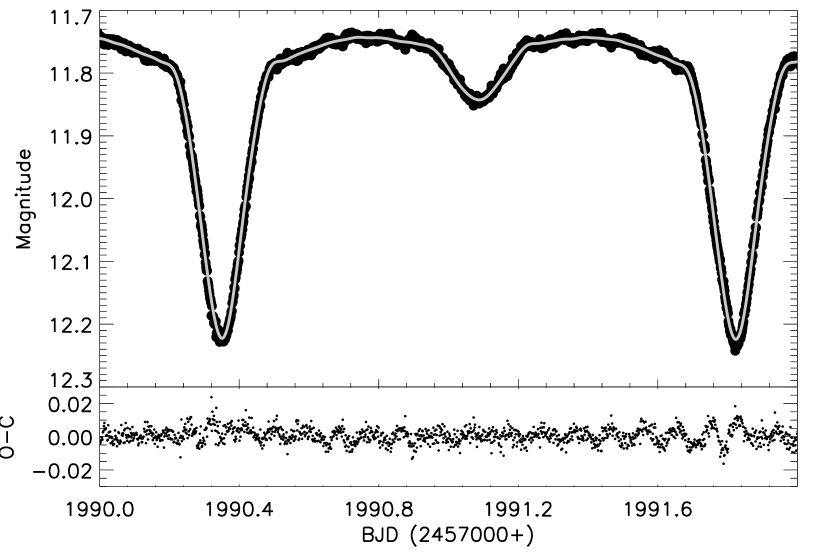
Figure 1: Upper panel: the fit (grey line) of the orbital frequency and its harmonics to the TESS data of TIC 85600400. Lower panel: residuals.

3 FREQUENCY ANALYSIS

In the current study, our main goal is revealing $\delta$ Scuti -type variations in our candidate systems. Therefore, we carried out a frequency analysis for each system. We used the Period04 program which derives individual frequencies from astronomical data including gaps and also allows us to find the combination and harmonic frequencies (Lenz & Breger, 2005). Our analysis consists of two steps. In the first step, the binary variations were removed from all available data of each target to obtain only the variation of oscillations. The binary variations were removed from the data with a phenomenological fit including the frequency of orbital periods and their harmonics (Kahraman Aliçavuş et al., 2022). Before starting this analysis, the orbital periods of each target were calculated by performing a frequency analysis and these orbital periods were used in the current research. We could not determine the orbital periods for some systems because there is only one primary eclipse in their data. The derived orbital parameters are given in Table 1. In Fig. 1, we show one example of orbital period frequency fits to the TESS data and the residuals. As clearly seen from the figure, the binary variations were extracted and only the light curve of the pulsations was obtained. In the light curves of some systems, there are only one or two eclipses in available data. For these systems, no orbital frequency fit was applied, only the eclipse(s) was removed from the light curves and the rest was analysed.

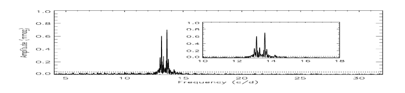
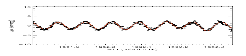
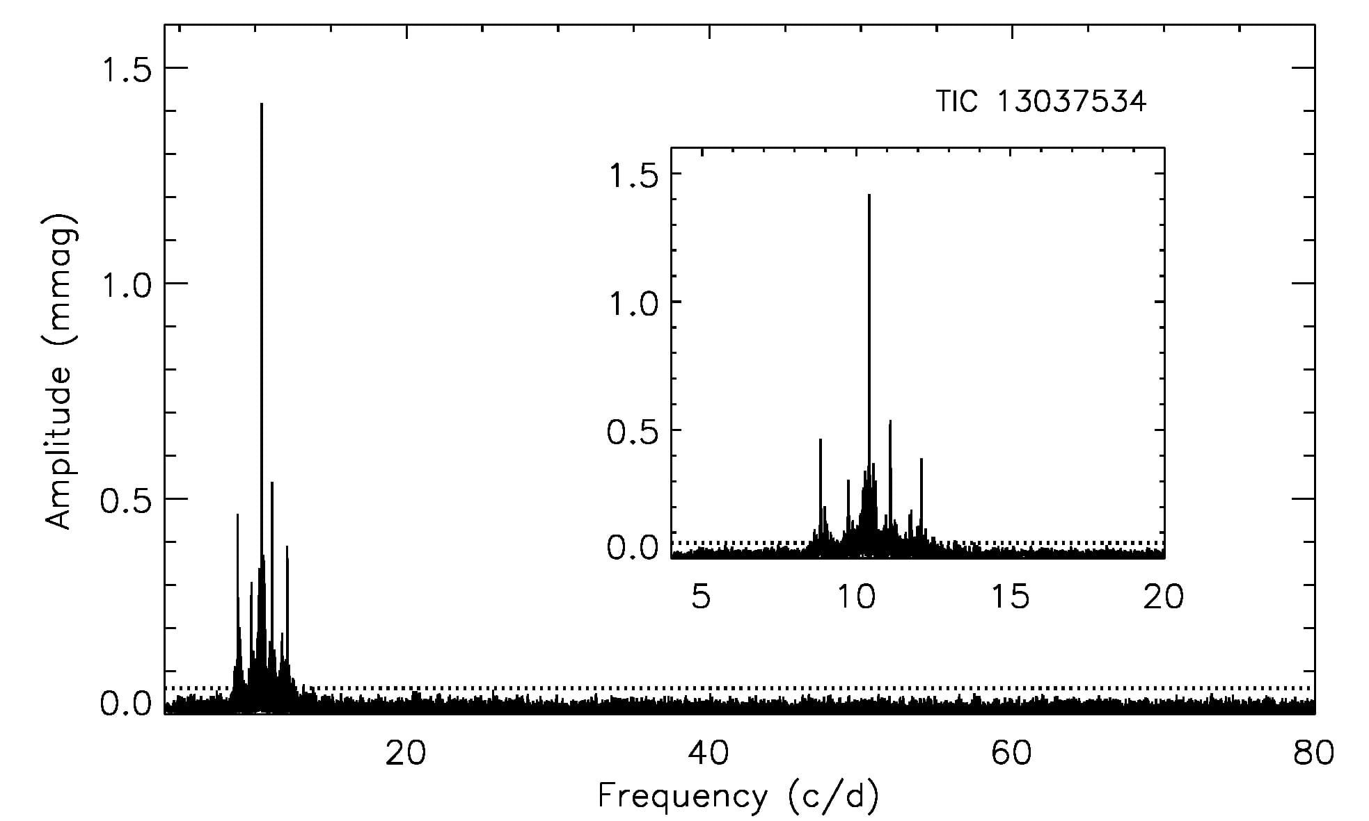
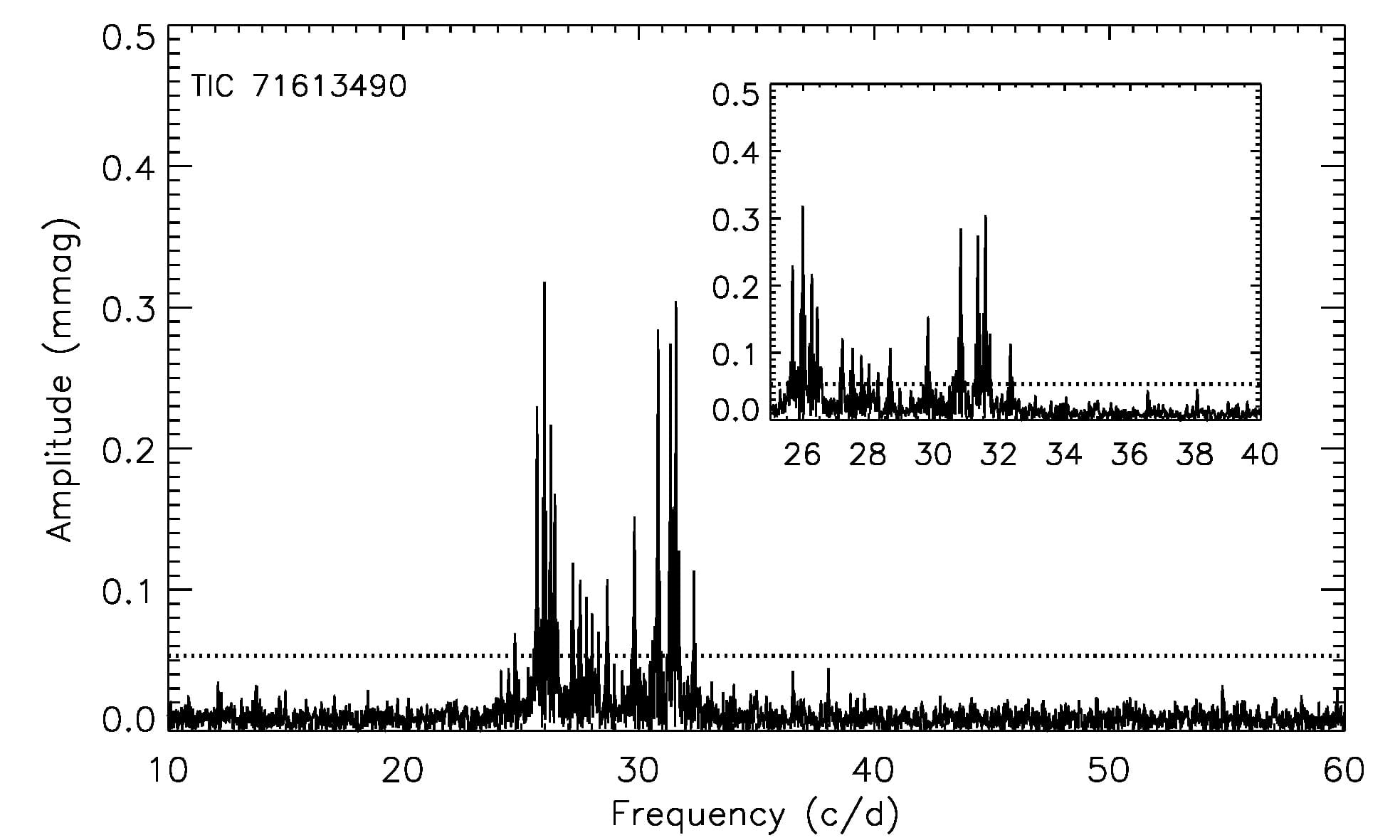
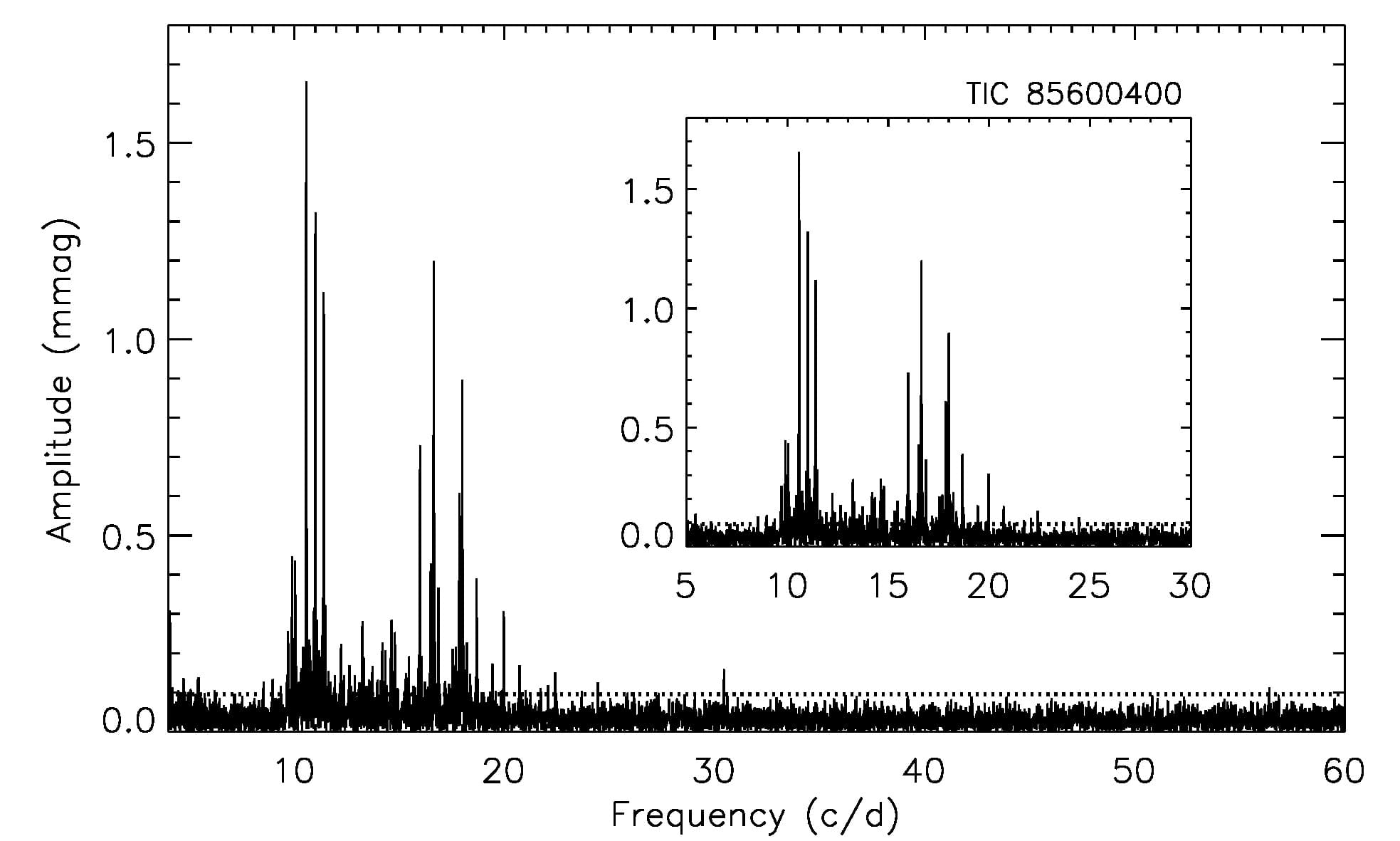
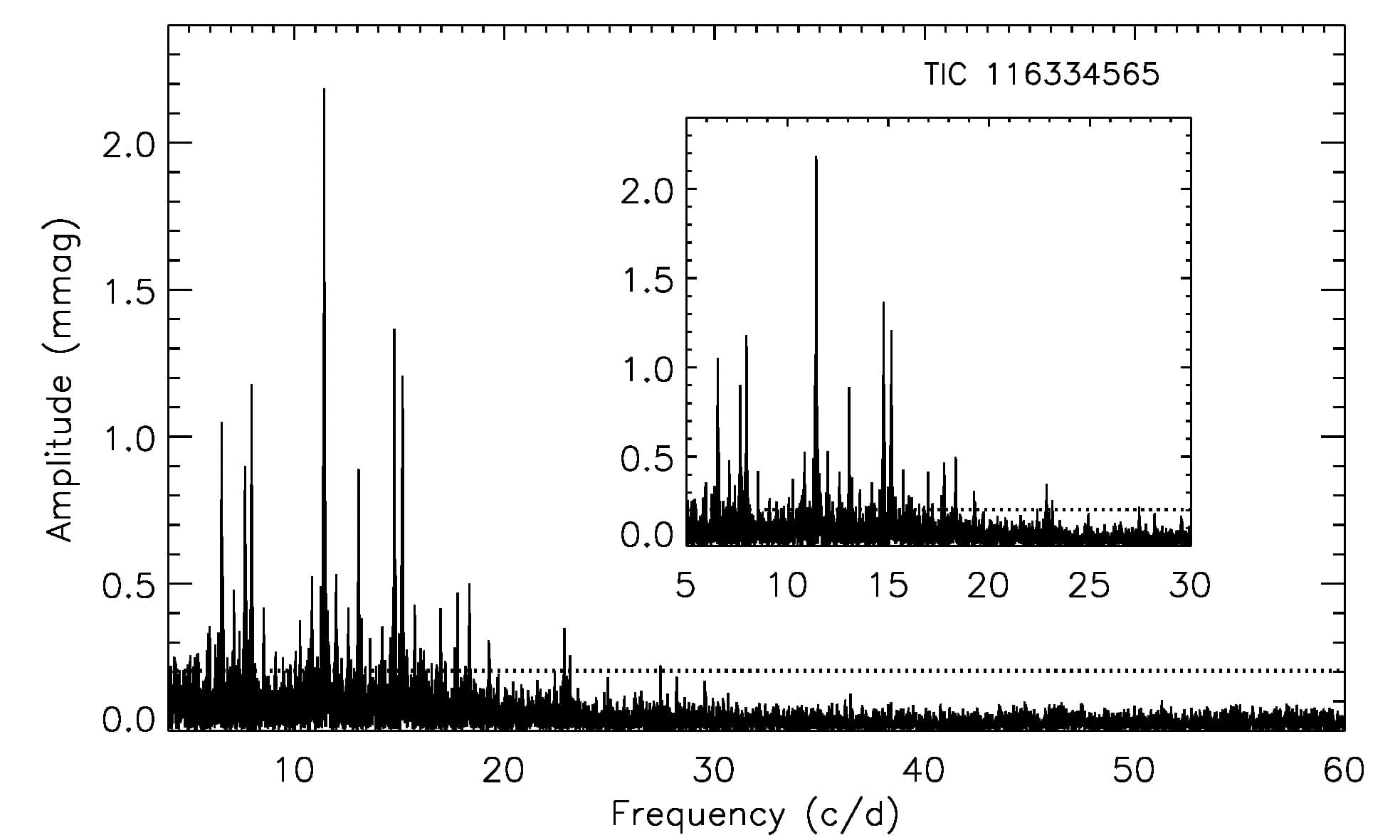
Figure 5: Amplitude spectra of the targets and the theoretical frequency fit (red solid lines) to the observations. Dotted lines represent the 4.5-$\sigma$ level.

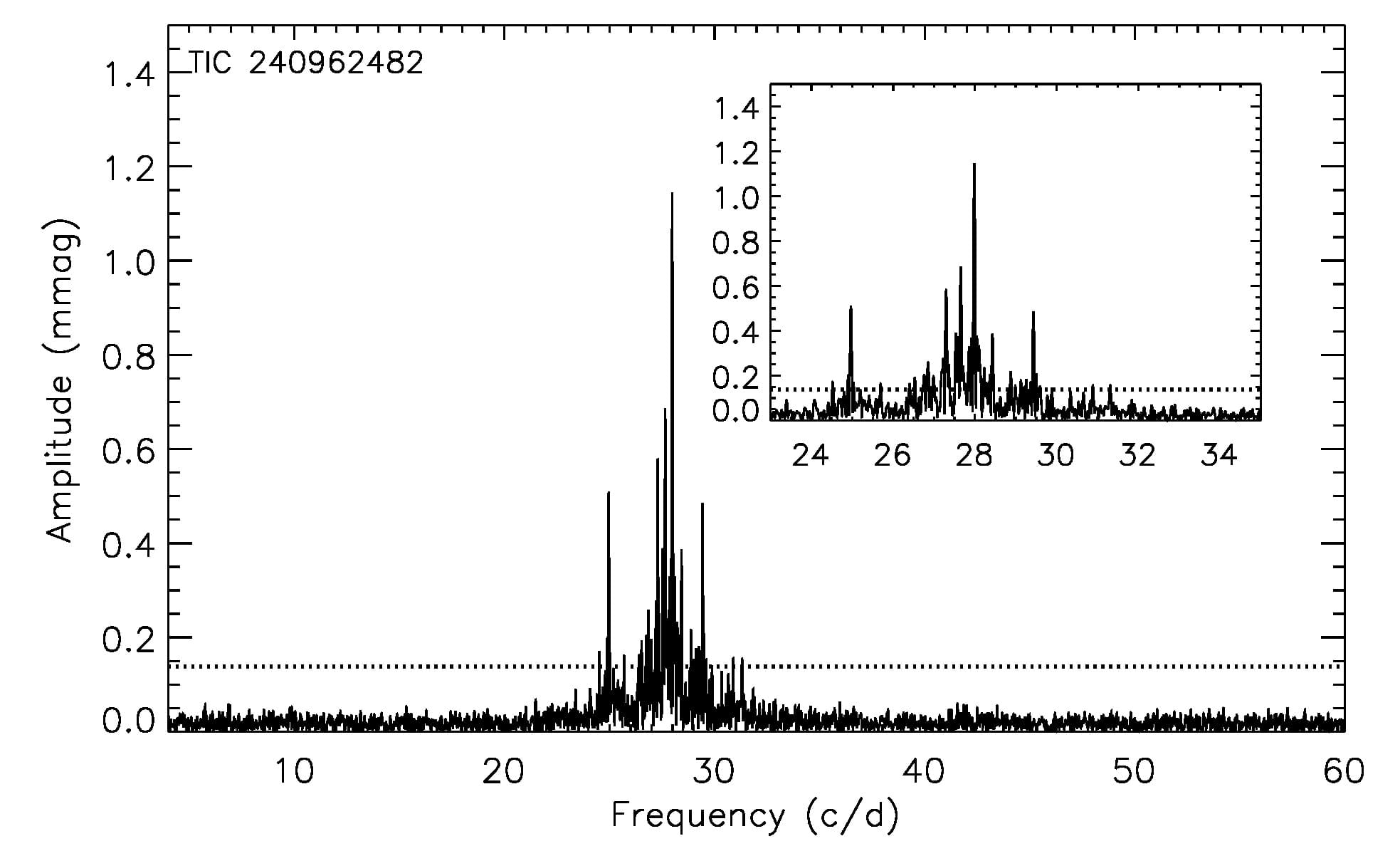
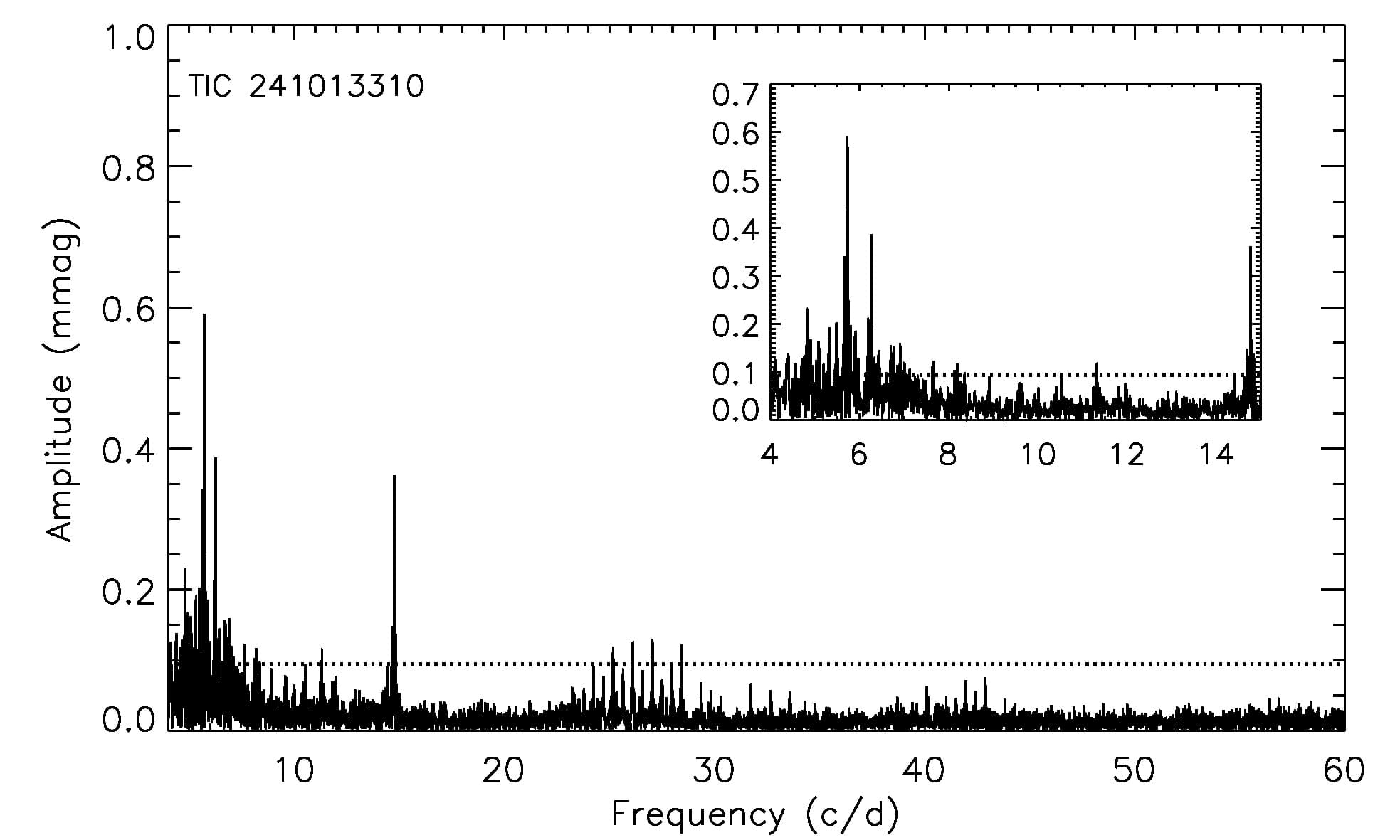
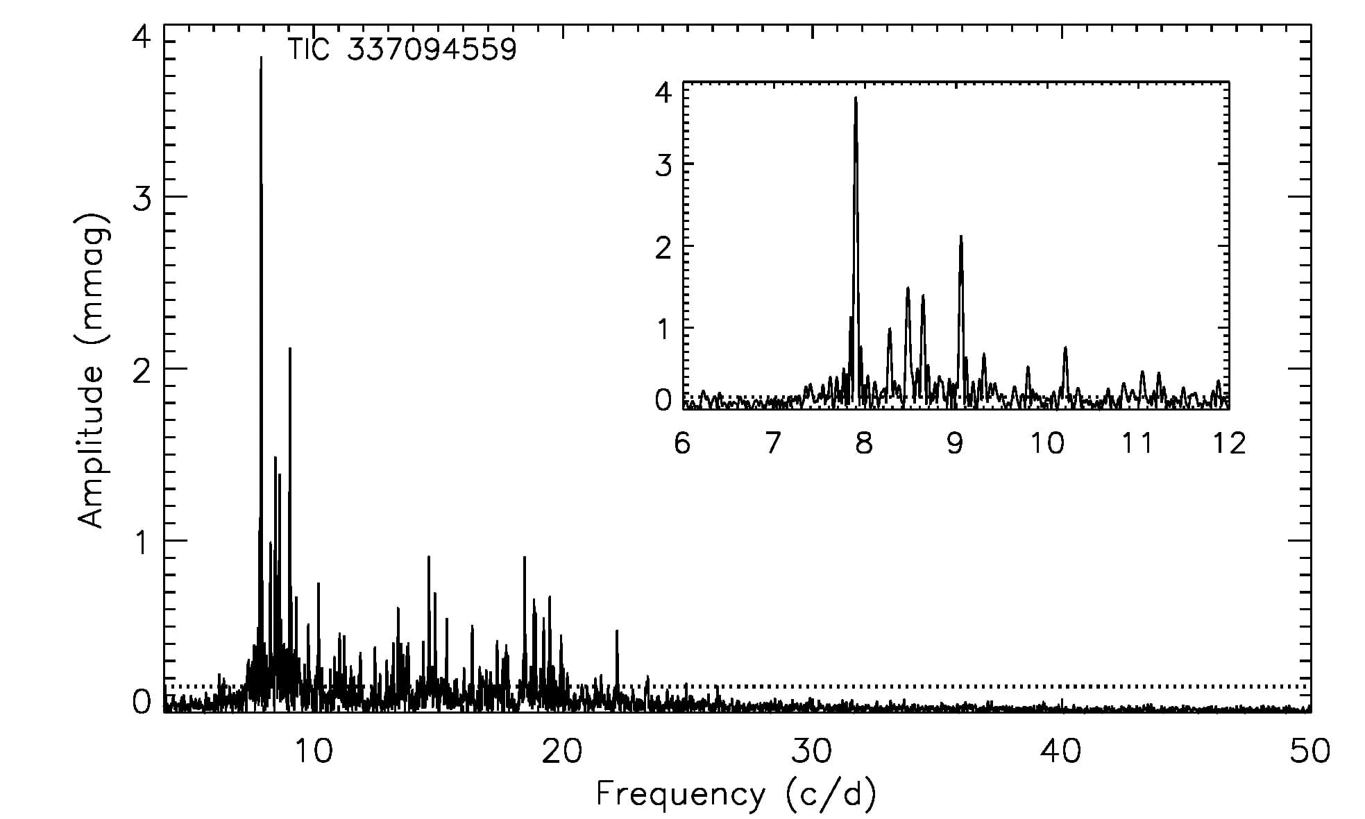
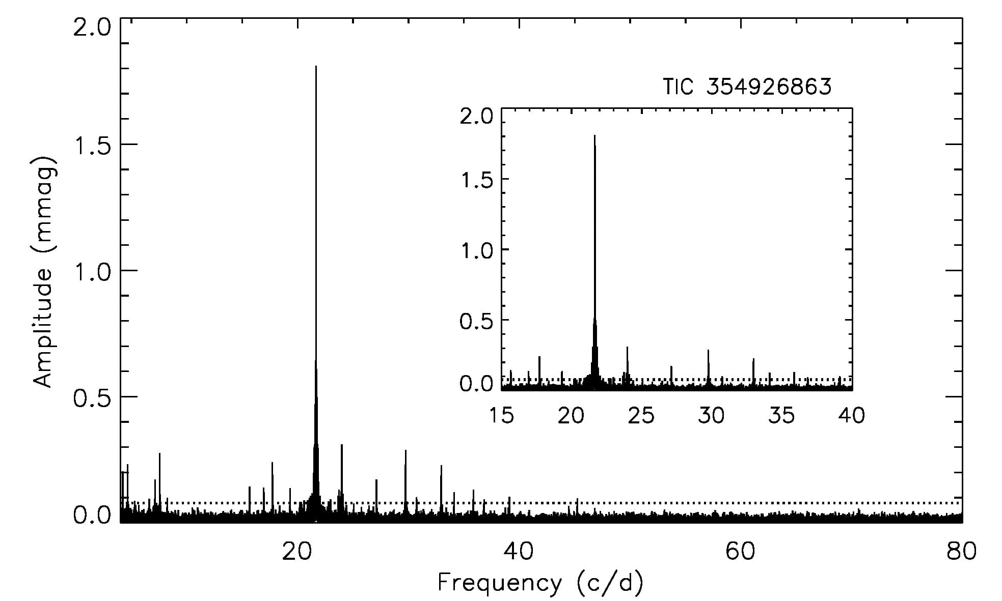
Figure 5: Continuation.

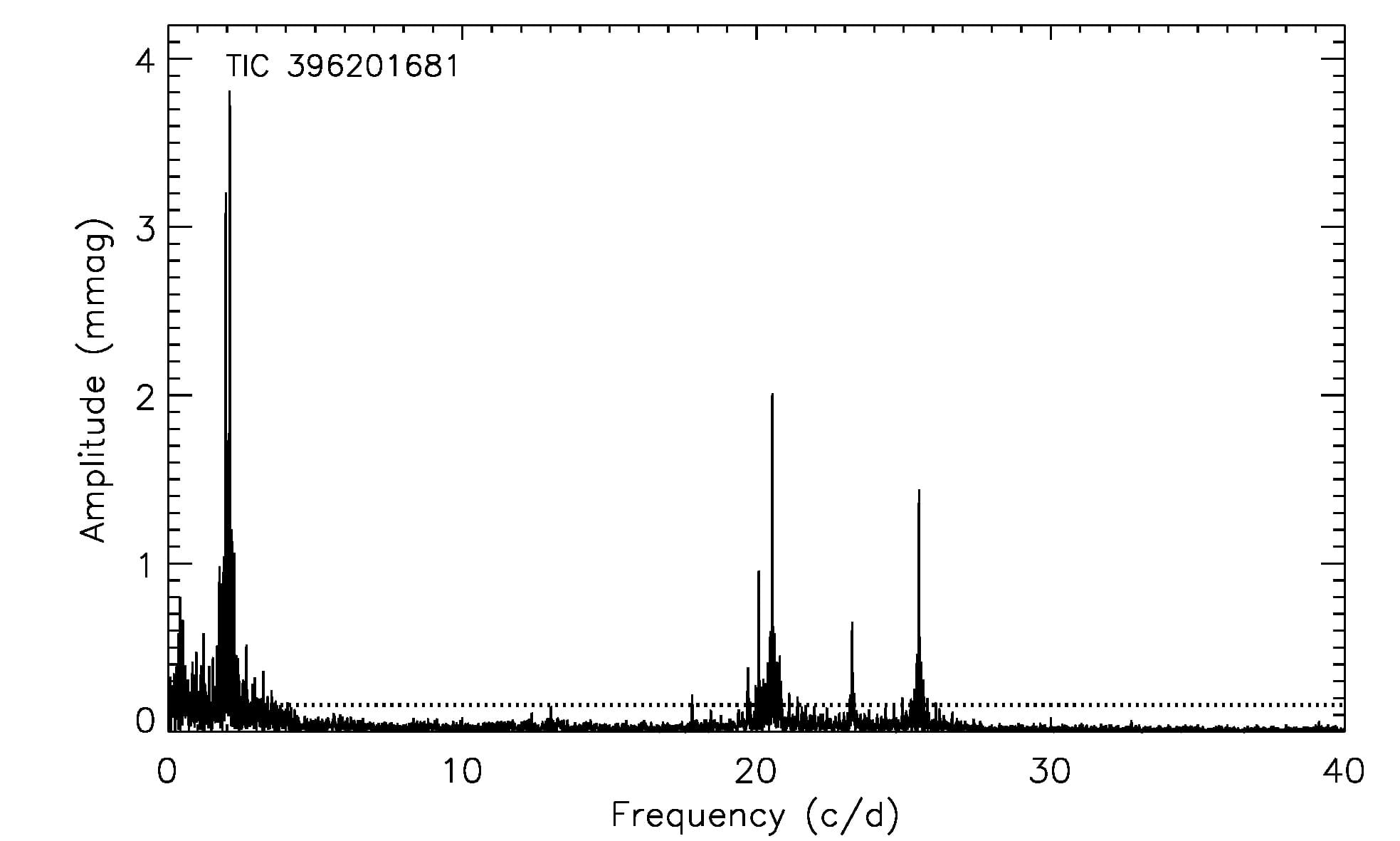
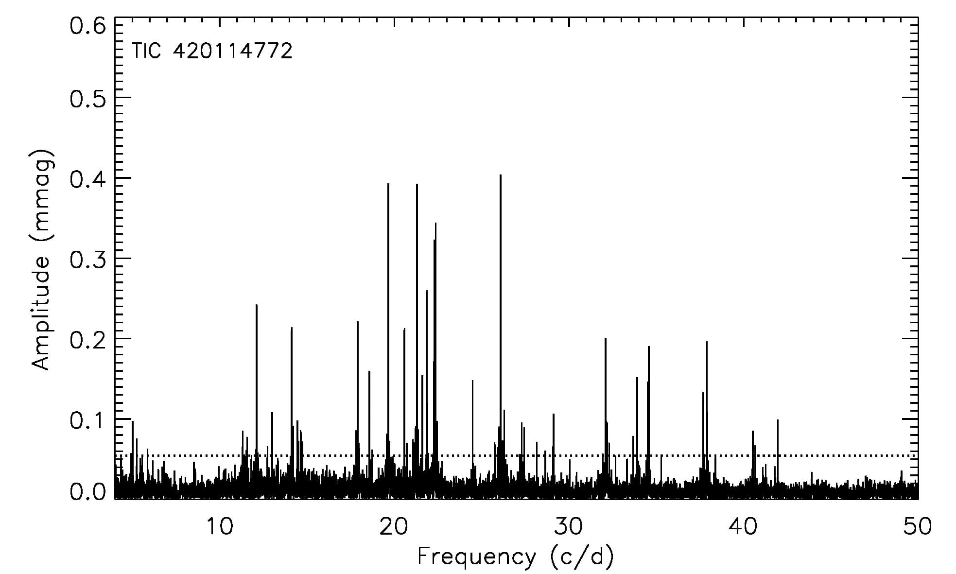
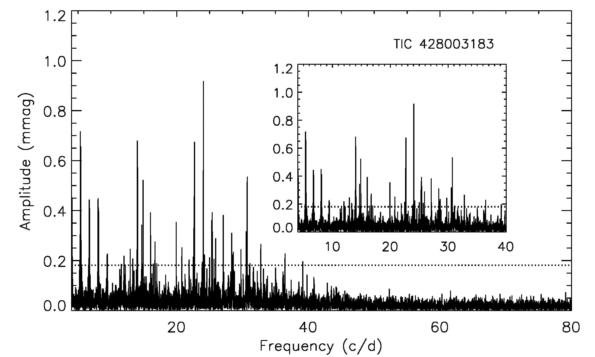
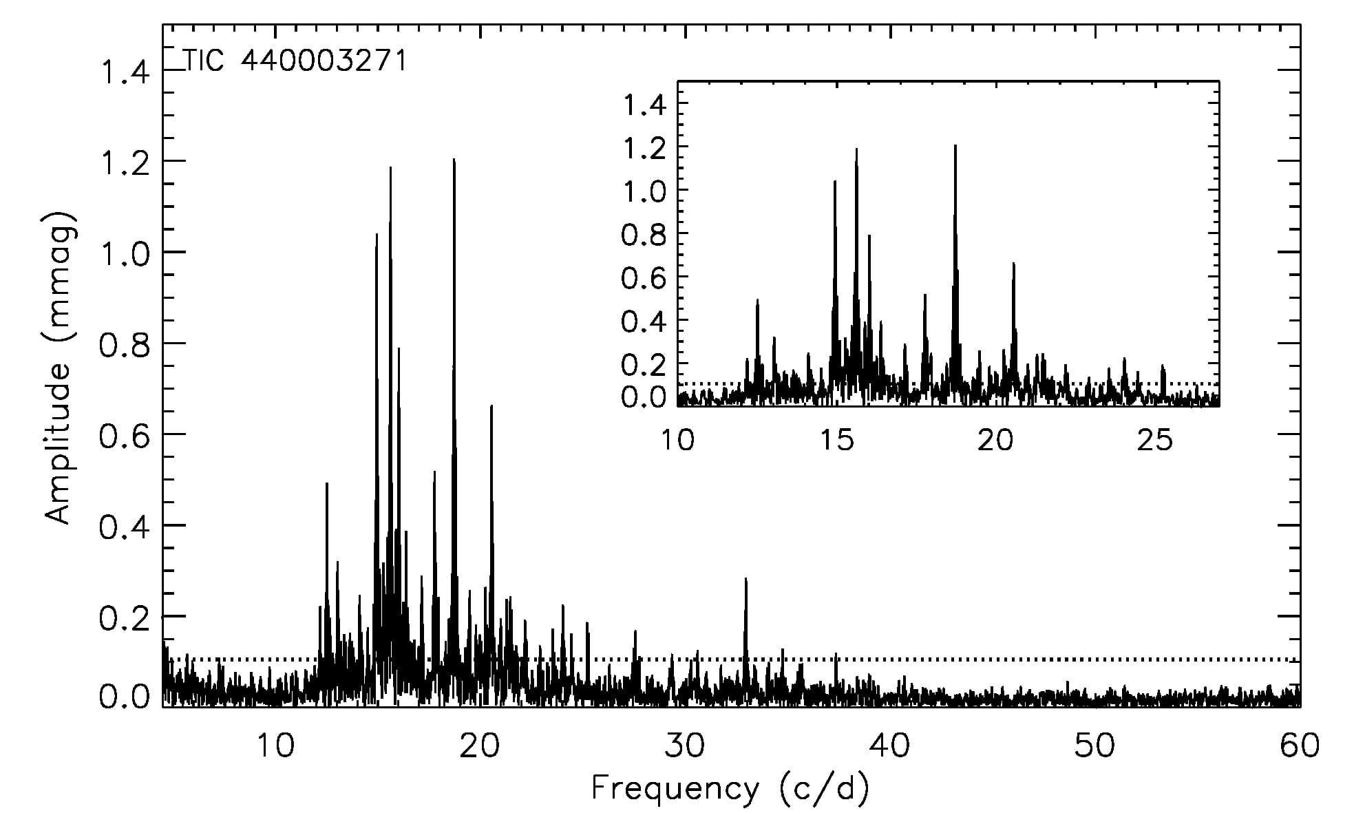
Figure 5: Continuation.

After the binary variations were removed from the TESS data of all targets, we carried out a frequency analysis of the residuals in the second step of the analysis. The independent, harmonic and combination frequencies were searched for. During the analysis, the frequencies having a signal-to-noise (S/N) ratio over 4.5 were expected as significant. A typical significance limit for the detected frequencies is given as 4.0 by Breger et al. (1993). However, Baran & Koen (2021) showed that this limit should be higher for TESS data and by taking into account the results obtained in their study, we took the significance limit as 4.5. The analysis was carried out for a range of $\sim$ $4-80$ $d^{-1}$ considering the typical pulsation period of $\delta$ Scuti  stars (see, Sect. LABEL:sec:int). One object in our targets (TIC 396201681) clearly show long-term $\gamma$ Doradus-type variation in its light curve. Therefore for this system the frequency analysis was performed for $\sim$ $0-80$ $d^{-1}$ range of frequency, as $\gamma$ Doradus stars typically exhibit pulsations with a frequency changing from $\sim$ 0.3 to 3 $d^{-1}$ (Aerts et al., 2010). Consequently, the range and the number of the detected frequencies are listed in Table 2. The first five highest amplitude frequencies are also given in Table 4 for each target. The full table is given in electronic form. The frequency spectrum and the fits of the calculated frequencies to the observations are shown in Fig. 2 for one sample and in Fig. 5 for the others.

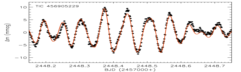
Figure 2: Left panel: the frequency spectrum of TIC 456905229. The dashed line represents the 4.5-$\sigma$ level. Right panel: theoretical fit (red solid line) to observed data (dots) for TIC 456905229.

4 CALCULATING PHYSICAL PARAMETERS

For all systems, we calculated some physical parameters such as luminosity ($L$), absolute ($M_{V}$) and bolometric ($M_{bol}$) magnitudes. However, one should keep in mind that these parameters represent the binary system and do not belong to only one binary component. Before starting to calculate these parameters, we estimated flux densities of binary components to estimate the flux contributions of each component to the total. It is known that the area ratio of eclipses approximately gives the flux density ratio of the binary components (Binnendijk, 1960). In the primary eclipse (deeper one) the loss of light is more than the secondary eclipse, so in the primary eclipse, the star with the higher surface luminosity hence hotter is obscured by other. We call this star as primary (p) and the other cool and less luminous one as secondary (s) component. The area of primary ($A_{p}$) and secondary ($A_{s}$) eclipses were measured by using IRAF(Tody, 1986) splot task. The ratio of these areas is equal to flux density ($I$) ratio as shown in the following equation (Binnendijk, 1960):

$$\frac{A_{p}}{A_{s}}\,=\,\frac{I_{p}}{I_{s}}$$ (1)

The calculated $I$ ratios are listed in Table 2. For some systems, there is only one eclipse available in the light curves, therefore flux ratio value could not be determined for these systems. As can be seen from the $I$ ratios, in most systems $I$ of the primary and secondary components close each other. We assumed that if the $I$ ratio is over $\sim$4 the calculated physical parameters mostly belong to the primary component.

The physical parameters of all systems were calculated using the distance module and the Pogson equation. To compute these parameters, the distances of the systems were taken from the Gaia EDR3 (Gaia Collaboration et al., 2021) and also extinction coefficient (A_υ) was calculated utilizing the interstellar extinction maps of Amôres & Lépine (2005). First the $M_{V}$ parameters were calculated by using the following equation:

$$V\,-\,M_{V}=5logd\,-\,5\,+\,A_{\upsilon}$$ (2)

where $V$ is the visual magnitude, d is the distance of the systems. After the $M_{V}$ values were derived the $M_{bol}$ parameters were computed taking into account the TIC $T_{\rm eff}$ values and bolometric corrections from Eker et al. (2020). If there is no $T_{\rm eff}$  value for a system we estimated this value from the target’s spectral type by using the calibration between the spectral type and $T_{\rm eff}$  given by Gray (1992). Additionally, for TIC 13037534, $T_{\rm eff}$  determined from the spectral type-$T_{\rm eff}$  calibration was used. Then, the $L$ parameters were computed with the below equation:

$$\frac{L}{L_{\odot}}\,=\,10^{(M_{bol\odot}\,-\,M_{bol})/2.5}$$ (3)

$M_{bol{\odot}}$ value is taken as 4^m.74 according to IAU 2015 General Assembly resolution B2. The calculated parameters are given in Table 2. Uncertainties of the computed parameters were estimated considering the errors in the input parameters. According to the $I$ ratio of the primary and secondary components, these calculated parameters mostly represents the binary systems. However, there are some systems in which the given $I$ ratio is over $\sim$4. In these systems the flux coming from the primary is significantly higher than the secondary and we assumed the calculated physical parameters mostly represents the hotter primary components and probably the pulsating one.

Table 2: Calculated Physical Parameters, $I$ Ratios of the Binary Components and the Range and the Number of the Detected Frequency. For TIC 430808126 Parameters could not be Calculated as It has no Parallax.

TIC	Aυ	$M_{V}$	$M_{bol}$	log (L/L⊙)	$I_{p}$/$I_{s}$	Frequency	Number of
number	(mag) $\pm$ 0.002	(mag)	(mag)			range ($d^{-1}$)	frequency
8669966	0.031	0.716 $\pm$ 0.025	0.767 $\pm$ 0.025	1.610 $\pm$ 0.045	1.23	13.103 $-$ 14.21	6
10057647	0.192	2.164 $\pm$ 0.032	2.237 $\pm$ 0.032	1.030 $\pm$ 0.052	1.40	13.77 $-$ 51.41	23
13037534	0.720	0.571 $\pm$ 0.025	0.588 $\pm$ 0.024	1.668 $\pm$ 0.045	6.64	8.84 $-$ 12.11	8
14948284	0.069	1.807 $\pm$ 0.024	1.883 $\pm$ 0.029	1.173 $\pm$ 0.044	1.20	8.09 $-$ 24.92	21
48084398	0.048	0.555 $\pm$ 0.029	0.635 $\pm$ 0.032	1.674 $\pm$ 0.049	1.04	8.98 $-$ 13.22	21
71613490	0.029	1.395 $\pm$ 0.032	1.441 $\pm$ 0.007	1.338 $\pm$ 0.052	1.04	24.47 $-$ 32.34	19
72839144	0.077	1.416 $\pm$ 0.007	1.492 $\pm$ 0.028	1.329 $\pm$ 0.027	3.55	4.11	1
75593781	0.708	1.364 $\pm$ 0.029	1.355 $\pm$ 0.016	1.350 $\pm$ 0.049	4.47	46.11 $-$ 57.94	15
78148497	0.663	1.324 $\pm$ 0.016	1.395 $\pm$ 0.032	1.367 $\pm$ 0.036	2.80	9.77 $-$ 32.97	22
85600400	0.087	1.651 $\pm$ 0.032	1.724 $\pm$ 0.027	1.236 $\pm$ 0.052	3.85	9.70 $-$ 19.97	17
116334565	0.809	0.849 $\pm$ 0.027	0.908 $\pm$ 0.031	1.557 $\pm$ 0.047	1.27	6.55 $-$ 22.85	12
165618747	0.298	2.107 $\pm$ 0.031	2.162 $\pm$ 0.011	1.053 $\pm$ 0.051	1.97	15.13 $-$ 40.18	28
172431974	0.047	1.557 $\pm$ 0.011	1.631 $\pm$ 0.032	1.273 $\pm$ 0.031	1.01	4.24 $-$ 6.40	10
193774939	0.080	2.220 $\pm$ 0.033	4.974 $\pm$ 0.019	1.008 $\pm$ 0.053	5.16	16.59 $-$ 31.21	21
197755658	0.029	2.074 $\pm$ 0.019	2.126 $\pm$ 0.013	1.066 $\pm$ 0.039	1.94	46.63 $-$ 51.26	3
197757000	0.123	2.576 $\pm$ 0.013	2.657 $\pm$ 0.009	0.865 $\pm$ 0.033	4.46	21.17 $-$ 41.98	21
240962482	0.190	1.689 $\pm$ 0.010	1.733 $\pm$ 0.007	1.221 $\pm$ 0.030	11.84	24.96 $-$ 29.43	5
241013310	0.110	2.335 $\pm$ 0.007	2.414 $\pm$ 0.033	0.962 $\pm$ 0.027	4.02	4.82 $-$ 14.77	4
256640561	0.079	0.823 $\pm$ 0.033	0.855 $\pm$ 0.007	1.567 $\pm$ 0.053	1.86	10.12 $-$ 24.42	12
272822330	0.165	0.997 $\pm$ 0.007	1.066 $\pm$ 0.030	1.497 $\pm$ 0.027	1.91	14.03 $-$ 20.34	11
289947843	0.083	0.912 $\pm$ 0.030	0.791 $\pm$ 0.012	1.531 $\pm$ 0.050	$-$	5.97 $-$ 14.44	11
301909087	0.624	1.137 $\pm$ 0.012	1.218 $\pm$ 0.026	1.441 $\pm$ 0.032	1.04	5.58 $-$ 17.44	10
305633328	0.245	1.680 $\pm$ 0.026	1.760 $\pm$ 0.014	1.224 $\pm$ 0.046	1.08	9.38 $-$ 15.37	8
322428763	0.174	1.441 $\pm$ 0.014	1.517 $\pm$ 0.022	1.483 $\pm$ 0.014	1.53	11.99 $-$ 49.78	11
327121759	0.726	1.374 $\pm$ 0.022	1.451 $\pm$ 0.011	1.346 $\pm$ 0.042	3.43	22.90 $-$ 30.97	6
337094559	0.097	2.049 $\pm$ 0.011	2.114 $\pm$ 0.061	1.077 $\pm$ 0.031	1.78	7.86 $-$ 19.47	8
338159479	0.292	2.332 $\pm$ 0.062	2.383 $\pm$ 0.011	0.963 $\pm$ 0.081	2.01	21.75 $-$ 28.51	17
354926863	0.298	2.755 $\pm$ 0.011	2.822 $\pm$ 0.007	0.794 $\pm$ 0.031	1.06	4.66 $-$ 39.11	18
358613523	0.097	2.813 $\pm$ 0.007	2.885 $\pm$ 0.034	0.771 $\pm$ 0.027	5.16	24.59 $-$ 46.44	15
393894013	0.044	2.216 $\pm$ 0.035	2.250 $\pm$ 0.023	1.010 $\pm$ 0.055	1.49	8.55 $-$ 69.65	19
396134795	0.628	1.290 $\pm$ 0.023	1.371 $\pm$ 0.038	1.380 $\pm$ 0.043	1.63	14.20 $-$ 28.47	7
396201681	0.184	1.595 $\pm$ 0.038	1.638 $\pm$ 0.071	1.258 $\pm$ 0.058	1.14	1.21 $-$ 23.52	11
420114772	0.127	0.656 $\pm$ 0.071	0.736 $\pm$ 0.016	1.634 $\pm$ 0.091	1.05	5.02 $-$ 41.95	30
421714420	0.097	-0.083 $\pm$ 0.016	-0.154 $\pm$ 0.014	1.929 $\pm$ 0.036	10.00	4.01 $-$ 53.19	11
428003183	0.106	2.438 $\pm$ 0.014	2.506 $\pm$ 0.015	0.921 $\pm$ 0.034	2.56	12.93 $-$ 32.77	22
430808126	$-$	$-$	$-$	$-$	1.07	5.26 $-$ 27.63	22
440003271	0.030	1.524 $\pm$ 0.026	1.510 $\pm$ 0.026	1.287 $\pm$ 0.046	1.10	12.19 $-$ 37.33	19
456905229	0.048	2.060 $\pm$ 0.074	2.139 $\pm$ 0.074	1.072 $\pm$ 0.094	1.12	10.13 $-$ 33.39	44
467354611	0.094	1.825 $\pm$ 0.023	1.166 $\pm$ 0.043	1.876 $\pm$ 0.027	$-$	11.58 $-$ 31.04	41

5 DISCUSSION

In this section, we examined some properties of our candidate DSEB.

5.1 Pulsation type

In this study, we present the analysis of some targets showing $\delta$ Scuti  like variations. While determining the candidate DSEB, one of the important criteria was the $T_{\rm eff}$  of the eclipsing binary systems. However, we know that these $T_{\rm eff}$  values are an average of both binary components. So real $T_{\rm eff}$  of pulsating components, could be higher or cooler than the TIC $T_{\rm eff}$. In some systems, we found that the primary components have significantly more flux density compared to secondary (see, Table 2). In these systems, the $T_{\rm eff}$  mostly represents the hotter primary and probably the pulsating components. When we examined the $T_{\rm eff}$  values of these systems, we found that their $T_{\rm eff}$  are in the range of the $T_{\rm eff}$  given for $\delta$ Scuti  stars. Their pulsation amplitudes and frequencies are also consistent with the values given for $\delta$ Scuti  stars (Aerts et al., 2010).

For the other systems which have the $I$ ratio lover than 4, probably the TIC $T_{\rm eff}$  values are substantially different than the real $T_{\rm eff}$  values of the pulsating components. Inside the pulsating stars, there are two different types that exhibit frequencies like $\delta$ Scuti  variables. One of them is $\beta$ Cephei stars. The $\beta$ Cephei stars mostly show frequencies between 3 and 12 $d^{-1}$ and these pulsators have $B0-B3$ spectral type (Aerts et al., 2010). Although these pulsators are quite hotter than the $\delta$ Scuti  variables, if a $\beta$ Cephei star have a very cool binary component, the total $T_{\rm eff}$  of the system will be cooler than the value expected for the $\beta$ Cephei stars. However, our targets have a $T_{\rm eff}$  value in a range of $\sim$ $6300-9100$ K and even if a $\beta$ Cephei star has a cool binary component, the average $T_{\rm eff}$  of the binary system could not as low as our targets’ $T_{\rm eff}$  range.

Another pulsating star group is Maia variables. The existence of Maia variables has not been exactly confirmed, however, for decades Maia variables are considered as a new group of pulsating stars (Aerts & Kolenberg, 2005; Balona et al., 2016; Balona & Ozuyar, 2020). The Maia variables are located between the $\beta$ Cephei and $\delta$ Scuti  stars, so they are cooler than $\beta$ Cephei variables and hotter than the $\delta$ Scuti  stars. Additionally, Maia variables demonstrate oscillations approximately in a similar frequency range with the $\delta$ Scuti stars (Balona et al., 2016; Balona & Ozuyar, 2020). Even the existence of Maia variables has not been approved, if they are a new type of variables, they could be a member of binary systems and seen cooler than expected if a Maia variable has a cooler binary component. In this case, they could be considered as a $\delta$ Scuti  variable. To have an idea about the variability type of our targets, their positions in the Hertzsprung-Russell (H-R) diagram should be examined by considering the $I$ ratios. Therefore, we showed the positions of our systems in the H-R diagram by using the parameters given in Table 1 and Table 2.

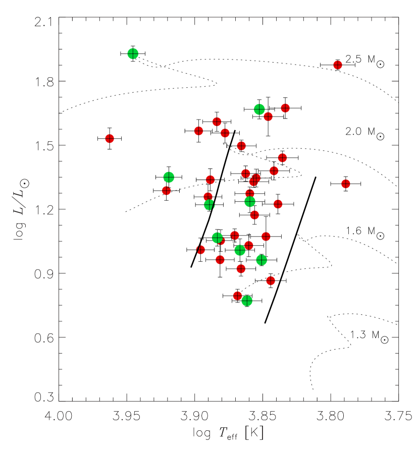
Figure 3: Positions of the targets in the H-R diagram. Green dots represent the systems having $I$ ratio higher than $\sim$ 4, while red smaller dots shows the other systems. The solid and dashed lines are the borders of the $\delta$ Scuti  instability strip (Dupret et al., 2005) and the evolutionary tracks taken from the MESA Isochrones and Stellar Tracks (MIST) (Paxton et al., 2011; Dotter, 2016; Choi et al., 2016), respectively.

As can be seen from Fig. 3, most of the systems, which have an $I$ ratio over around 4, are located in the $\delta$ Scuti  instability strip and for these systems, we assumed the $L$ and $T_{\rm eff}$  mostly represent the primary, probably the pulsating, binary component. Inside these systems, there is one object (TIC 421714420) that is placed beyond the hot border of $\delta$ Scuti  instability strip. In a detailed study of Kepler field $\delta$ Scuti  and related stars, Uytterhoeven et al. (2011) showed that there are some real $\delta$ Scuti  variables located beyond the borders of the $\delta$ Scuti  instability strip. However, this system is noticeable far from the $\delta$ Scuti  instability strip, and very close to the place where Maia variables are located (Balona & Ozuyar, 2020). Therefore we classified this system as a candidate of Maia variable in an eclipsing binary. There is another system located beyond the hotter border of $\delta$ Scuti  stars, TIC 289947843, unfortunately, we could not measure the $I$ ratio for this system because there is not enough data. For the other systems having $I$ ratio $<$4 the $L$ value of the pulsating component should be lower than the calculated one and depending on $T_{\rm eff}$  of the other binary component the $T_{\rm eff}$  of the pulsating star could be lower or higher than the used in the H-R diagram. Taking into account these conditions, we could say that most pulsating components could be located inside the $\delta$ Scuti  instability strip however it is difficult to have an idea about the variability of the systems considering this. Therefore, as a result of this examination, we classified 38 systems as candidate DSEB and one of them, TIC 421714420, as a Maia candidate in an eclipsing binary system.

5.2 Consistency with the known relationship for DSEBs

DSEB have been investigated for a long time and it was shown that there are some relationships between the pulsation period, amplitude and the other parameters such as $P_{orb}$, $R$ and $\log g$ (Kahraman Aliçavuş et al., 2017; Liakos & Niarchos, 2017). For DSEB, the well-known relationship is between the P_orb and P_puls. In the latest study of Kahraman Aliçavuş et al. (2017), it was shown that known DSEB obey this relationship within error bars. We examined whether our candidate systems suit this relationship. In this section, we only investigate the candidate DSEB. As can be seen from Fig.4, most of our candidates are consistent with the relationship within errors. There are a few objects placed outside of the 1-$\sigma$ level, TIC 72839144, TIC 172431974, TIC 197755658 and TIC 241013310. The reason for these could be the additional effect in the binary system such as mass transfer between binary components if these systems are DSEB.

Figure 4: Consistency of the candidate DSEB with P_orb $-$ P_puls relationship. The filled and empty circles represent our candidate and the known DSEB (Kahraman Aliçavuş et al., 2017), respectively. The solid and dashed lines show the correlation and 1-$\sigma$ level, respectively.

More relationships between the P_puls and other parameters are given by Kahraman Aliçavuş et al. (2017) for detached and semi-detached systems. These parameters help us approximately estimate some physical parameters of the $\delta$ Scuti  pulsating components in eclipsing binary systems. As we do not know the Roche geometry of our systems we could not classify the binary configurations of our targets. However, for both detached and semi-detached binary configurations, some relationships give a good correlation between the P_puls such as $\log g$  and radius ($R$) of the pulsating component. Therefore, we calculated $\log g$  and $R$ parameters of our systems using the equations given in the study of Kahraman Aliçavuş et al. (2017). In this calculation, we excluded the systems found outside of the P_orb $-$ P_puls relationship. The computed $\log g$  and $R$ parameters are listed in Table 3. By utilizing the calculated $\log g$  and $R$, we also estimated the mass ($M$) values of the pulsating component. These values are also given in Table 3. It should keep in mind that these parameters are just an estimation and do not give exact values and the real errors should be higher.

Table 3: Calculated Parameters from the Given Relationships by Kahraman Aliçavuş et al. (2017).

TIC	$\log g$	$R$	$M$
number	(cgs)	($R_{\odot}$)	($M_{\odot}$)
8669966	3.65 $\pm$ 0.20	3.53 $\pm$ 0.39	2.07 $\pm$ 0.30
10057647	4.41 $\pm$ 0.24	1.39 $\pm$ 0.24	1.85 $\pm$ 0.38
13037534	3.51 $\pm$ 0.28	3.93 $\pm$ 0.51	1.85 $\pm$ 0.40
14948284	3.93 $\pm$ 0.10	2.74 $\pm$ 0.32	2.38 $\pm$ 0.10
48084398	3.56 $\pm$ 0.26	3.80 $\pm$ 0.47	1.93 $\pm$ 0.36
71613490	4.10 $\pm$ 0.11	2.25 $\pm$ 0.05	2.39 $\pm$ 0.06
75593781	4.59 $\pm$ 0.34	0.88 $\pm$ 0.39	1.13 $\pm$ 0.36
78148497	3.59 $\pm$ 0.24	3.70 $\pm$ 0.44	1.98 $\pm$ 0.34
116334565	3.53 $\pm$ 0.28	3.87 $\pm$ 0.49	1.88 $\pm$ 0.38
165618747	4.37 $\pm$ 0.22	1.52 $\pm$ 0.20	1.97 $\pm$ 0.34
193774939	3.97 $\pm$ 0.12	2.62 $\pm$ 0.12	2.40 $\pm$ 0.19
197757000	4.35 $\pm$ 0.20	1.57 $\pm$ 0.18	2.03 $\pm$ 0.30
240962482	4.16 $\pm$ 0.14	2.10 $\pm$ 0.03	2.36 $\pm$ 0.09
256640561	3.44 $\pm$ 0.32	4.11 $\pm$ 0.56	1.75 $\pm$ 0.44
272822330	3.79 $\pm$ 0.12	3.14 $\pm$ 0.28	2.25 $\pm$ 0.20
289947843	3.69 $\pm$ 0.18	3.41 $\pm$ 0.36	2.13 $\pm$ 0.28
301909087	3.64 $\pm$ 0.22	3.57 $\pm$ 0.40	2.05 $\pm$ 0.32
305633328	3.45 $\pm$ 0.32	4.10 $\pm$ 0.56	1.75 $\pm$ 0.44
322428763	3.59 $\pm$ 0.24	3.70 $\pm$ 0.44	1.98 $\pm$ 0.34
327121759	4.04 $\pm$ 0.10	2.44 $\pm$ 0.17	2.41 $\pm$ 0.22
338159479	4.13 $\pm$ 0.10	2.17 $\pm$ 0.01	2.38 $\pm$ 0.09
354926863	3.98 $\pm$ 0.10	2.61 $\pm$ 0.12	2.40 $\pm$ 0.17
358613523	4.43 $\pm$ 0.26	1.32 $\pm$ 0.26	1.77 $\pm$ 0.42
393894013	4.44 $\pm$ 0.26	1.30 $\pm$ 0.26	1.74 $\pm$ 0.44
396134795	3.68 $\pm$ 0.10	3.44 $\pm$ 0.37	2.11 $\pm$ 0.28
396201681	3.94 $\pm$ 0.10	2.72 $\pm$ 0.15	2.38 $\pm$ 0.17
420114772	4.11 $\pm$ 0.10	2.24 $\pm$ 0.05	2.39 $\pm$ 0.07
421714420	4.27 $\pm$ 0.16	1.78 $\pm$ 0.24	2.20 $\pm$ 0.22
428003183	4.05 $\pm$ 0.10	2.40 $\pm$ 0.06	2.41 $\pm$ 0.11
430808126	3.81 $\pm$ 0.06	3.09 $\pm$ 0.26	2.27 $\pm$ 0.18
440003271	3.87 $\pm$ 0.14	2.90 $\pm$ 0.21	2.34 $\pm$ 0.14
456905229	3.73 $\pm$ 0.16	3.31 $\pm$ 0.33	2.18 $\pm$ 0.24
467354611	3.71 $\pm$ 0.16	3.35 $\pm$ 0.34	2.16 $\pm$ 0.26

6 CONCLUSIONS

In this study, we present the results of our northern TESS field search to discover new eclipsing binaries with $\delta$ Scuti  components. We first determined 39 targets and examined the pulsational properties (pulsation amplitude and frequencies) of these systems after removing the eclipsing variations. In addition to determining pulsation amplitude and frequencies, we also estimated the $I$ ratios of binary components to find how much binary components contribute to total flux relative to each other. To estimate whether our systems could be DSEB or not, we also controlled the positions of the targets in the H-R diagram. For this, we calculated $L$ parameters of the systems. By considering the positions of the systems in the H-R diagram and the $I$ ratios, we showed that one of our targets (TIC 421714420) could be a candidate of Maia variable in an eclipsing binary system. The other targets in the study are classified as candidate DSEB. However, to be sure about the positions of the systems in the H-R diagram and the real $T_{\rm eff}$  values of them, detailed spectroscopic analysis and binary modelling are necessary. With the spectroscopy the $T_{\rm eff}$  value of each binary component can be derived and with the binary modelling, the real $L$ parameters could be reached.

We know that the pulsating eclipsing binary systems are quite important to deeply understand stellar systems. An increasing number of these kinds of systems would contribute to improving our knowledge about the stellar evolution and structure. Therefore, this study would be useful for both probing stellar structure, evolution and understanding the pulsation behaviour of oscillating stars in eclipsing binary systems.

Table 4: The List of the First Five Highest Amplitude Frequency Detected in This Study. The Full List of the Frequencies is Given in Electronic Form.

	Frequency	Amplitude	Phase	S/N		Frequency	Amplitude	Phase	S/N		Frequency	Amplitude	Phase	S/N
	(d-1)	(mmag)	(rad)			(d-1)	(mmag)	(rad)			(d-1)	(mmag)	(rad)
TIC 8669966					TIC 10057647					TIC 13037534
$\nu_{1}$	13.62189 $\pm$ 0.00015	0.717 $\pm$ 0.005	0.5562 $\pm$ 0.0011	62	$\nu_{1}$	40.11281 $\pm$ 0.00019	0.727 $\pm$ 0.007	0.2288 $\pm$ 0.0015	54	$\nu_{1}$	11.10889 $\pm$ 0.00004	0.526 $\pm$ 0.012	0.8332 $\pm$ 0.0036	20
$\nu_{2}$	13.14363 $\pm$ 0.00017	0.618 $\pm$ 0.005	0.0358 $\pm$ 0.0013	61	$\nu_{2}$	30.95924 $\pm$ 0.00020	0.686 $\pm$ 0.007	0.1324 $\pm$ 0.0015	69	$\nu_{2}$	8.84272 $\pm$ 0.00006	0.459 $\pm$ 0.012	0.3634 $\pm$ 0.0048	24
$\nu_{3}$	13.32788 $\pm$ 0.00038	0.278 $\pm$ 0.005	0.0784 $\pm$ 0.0028	26	$\nu_{3}$	38.78309 $\pm$ 0.00028	0.481 $\pm$ 0.007	0.8545 $\pm$ 0.0022	31	$\nu_{3}$	9.74327 $\pm$ 0.00006	0.323 $\pm$ 0.012	0.4381 $\pm$ 0.0055	13
$\nu_{4}$	13.03191 $\pm$ 0.00042	0.251 $\pm$ 0.005	0.0809 $\pm$ 0.0031	25	$\nu_{4}$	43.60348 $\pm$ 0.00034	0.399 $\pm$ 0.007	0.4591 $\pm$ 0.0027	28	$\nu_{4}$	10.63240 $\pm$ 0.00015	0.210 $\pm$ 0.012	0.2293 $\pm$ 0.0045	8
$\nu_{5}$	13.73165 $\pm$ 0.00049	0.217 $\pm$ 0.005	0.5787 $\pm$ 0.0036	19	$\nu_{5}$	36.01630 $\pm$ 0.00048	0.283 $\pm$ 0.007	0.6612 $\pm$ 0.0037	24	$\nu_{5}$	10.41897 $\pm$ 0.00026	0.207 $\pm$ 0.019	0.8755 $\pm$ 0.0495	8
TIC 14948284				TIC 48084398					TIC 71613490
$\nu_{1}$	20.31697 $\pm$ 0.00019	3.130 $\pm$ 0.028	0.7751 $\pm$ 0.0014	22	$\nu_{1}$	11.88739 $\pm$ 0.00006	1.099 $\pm$ 0.006	0.5054 $\pm$ 0.0008	30	$\nu_{1}$	25.98838 $\pm$ 0.00049	0.323 $\pm$ 0.007	0.9887 $\pm$ 0.0035	24
$\nu_{2}$	11.20278 $\pm$ 0.00021	2.776 $\pm$ 0.028	0.1298 $\pm$ 0.0016	20	$\nu_{2}$	9.49467 $\pm$ 0.00006	1.009 $\pm$ 0.006	0.9585 $\pm$ 0.0009	24	$\nu_{2}$	31.57531 $\pm$ 0.00054	0.289 $\pm$ 0.007	0.8029 $\pm$ 0.0039	26
$\nu_{3}$	20.11472 $\pm$ 0.00038	1.567 $\pm$ 0.028	0.5509 $\pm$ 0.0029	11	$\nu_{3}$	11.41491 $\pm$ 0.00007	0.861 $\pm$ 0.006	0.9264 $\pm$ 0.0010	25	$\nu_{3}$	30.81604 $\pm$ 0.00057	0.274 $\pm$ 0.007	0.2540 $\pm$ 0.0041	23
$\nu_{4}$	18.05449 $\pm$ 0.00038	1.541 $\pm$ 0.028	0.0802 $\pm$ 0.0029	16	$\nu_{2}$+$\nu_{3}$-$\nu_{1}$	9.02219 $\pm$ 0.00008	0.784 $\pm$ 0.006	0.3972 $\pm$ 0.0011	19	$\nu_{4}$	31.33778 $\pm$ 0.00061	0.257 $\pm$ 0.007	0.7478 $\pm$ 0.0043	22
$\nu_{5}$	17.67646 $\pm$ 0.00048	1.247 $\pm$ 0.028	0.1414 $\pm$ 0.0036	14	$\nu_{5}$	11.02949 $\pm$ 0.00010	0.632 $\pm$ 0.006	0.1951 $\pm$ 0.0014	18	$\nu_{5}$	26.25839 $\pm$ 0.00065	0.242 $\pm$ 0.007	0.9569 $\pm$ 0.0046	15
TIC 72839144				TIC 75593781					TIC 78148497
$\nu_{1}$	4.11102 $\pm$ 0.00133	0.328 $\pm$ 0.020	0.8042 $\pm$ 0.0098	6.0	$\nu_{1}$	51.91704 $\pm$ 0.00011	1.544 $\pm$ 0.023	0.1718 $\pm$ 0.0024	46	$\nu_{1}$	12.44590 $\pm$ 0.00009	1.383 $\pm$ 0.017	0.3311 $\pm$ 0.0020	39
					$\nu_{2}$	48.85966 $\pm$ 0.00018	0.914 $\pm$ 0.023	0.8996 $\pm$ 0.0040	30	$\nu_{2}$	16.39778 $\pm$ 0.00014	0.900 $\pm$ 0.017	0.5090 $\pm$ 0.0031	19
					$\nu_{3}$	52.40034 $\pm$ 0.00022	0.754 $\pm$ 0.023	0.5367 $\pm$ 0.0048	22	$\nu_{3}$	24.48400 $\pm$ 0.00019	0.662 $\pm$ 0.017	0.2477 $\pm$ 0.0042	16
					$\nu_{4}$	47.75704 $\pm$ 0.00028	0.588 $\pm$ 0.023	0.1146 $\pm$ 0.0062	20	$\nu_{4}$	23.67636 $\pm$ 0.00018	0.677 $\pm$ 0.017	0.9442 $\pm$ 0.0041	16
					$\nu_{5}$	50.61103 $\pm$ 0.00026	0.622 $\pm$ 0.023	0.7971 $\pm$ 0.0058	19	$\nu_{5}$	26.07247 $\pm$ 0.00020	0.616 $\pm$ 0.017	0.5684 $\pm$ 0.0045	17
TIC 85600400					TIC 116334565					TIC 165618747
$\nu_{1}$	10.57549 $\pm$ 0.00018	1.666 $\pm$ 0.027	0.6049 $\pm$ 0.0026	29	$\nu_{1}$	11.42838 $\pm$ 0.00007	2.212 $\pm$ 0.117	0.4961 $\pm$ 0.0005	36	$\nu_{1}$	37.87282 $\pm$ 0.00039	0.765 $\pm$ 0.025	0.5868 $\pm$ 0.0060	23
$\nu_{2}$	11.01141 $\pm$ 0.00021	1.386 $\pm$ 0.027	0.2475 $\pm$ 0.0031	24	$\nu_{2}$	14.76193 $\pm$ 0.00007	1.360 $\pm$ 0.117	0.8032 $\pm$ 0.0005	20	$\nu_{2}$	37.54370 $\pm$ 0.00039	0.675 $\pm$ 0.025	0.4108 $\pm$ 0.0059	20
$\nu_{3}$	16.63944 $\pm$ 0.00025	1.171 $\pm$ 0.027	0.3368 $\pm$ 0.0037	22	$\nu_{3}$	15.15892 $\pm$ 0.00008	0.1207 $\pm$ 0.117	0.7195 $\pm$ 0.0006	17	$\nu_{3}$	35.11748 $\pm$ 0.00060	0.474 $\pm$ 0.025	0.1010 $\pm$ 0.0090	14
$\nu_{4}$	11.39975 $\pm$ 0.00025	1.183 $\pm$ 0.027	0.8613 $\pm$ 0.0037	20	$\nu_{4}$	7.97122 $\pm$ 0.00010	1.212 $\pm$ 0.117	0.7470 $\pm$ 0.0007	17	$\nu_{4}$	23.54175 $\pm$ 0.00056	0.430 $\pm$ 0.025	0.9865 $\pm$ 0.0084	14
$\nu_{5}$	17.99572 $\pm$ 0.00030	0.971 $\pm$ 0.027	0.3860 $\pm$ 0.0045	22	$\nu_{5}$	6.54611 $\pm$ 0.00012	1.073 $\pm$ 0.117	0.7175 $\pm$ 0.0008	13	$\nu_{5}$	30.49806 $\pm$ 0.00069	0.414 $\pm$ 0.025	0.6068 $\pm$ 0.0103	12

Table 4: Continuation.

	Frequency	Amplitude	Phase	S/N		Frequency	Amplitude	Phase	S/N		Frequency	Amplitude	Phase	S/N
	(d-1)	(mmag)	(rad)			(d-1)	(mmag)	(rad)			(d-1)	(mmag)	(rad)
TIC 172431974					TIC 193774939					TIC 197755658
$\nu_{1}$	5.32323 $\pm$ 0.00015	1.854 $\pm$ 0.026	0.3324 $\pm$ 0.0022	42	$\nu_{1}$	21.59652 $\pm$ 0.00014	0.825 $\pm$ 0.010	0.6836 $\pm$ 0.0020	38	$\nu_{1}$	51.25620 $\pm$ 0.00044	0.562 $\pm$ 0.024	0.9177 $\pm$ 0.0067	22
$\nu_{2}$	4.27899 $\pm$ 0.00053	0.528 $\pm$ 0.026	0.5921 $\pm$ 0.0078	7	$\nu_{2}$	26.67014 $\pm$ 0.00014	0.783 $\pm$ 0.010	0.7211 $\pm$ 0.0021	45	$\nu_{2}$	46.63643 $\pm$ 0.00080	0.310 $\pm$ 0.024	0.7649 $\pm$ 0.0121	11
$\nu_{3}$	5.12970 $\pm$ 0.00054	0.443 $\pm$ 0.026	0.6626 $\pm$ 0.0093	10	$\nu_{3}$	16.69181 $\pm$ 0.00017	0.642 $\pm$ 0.010	0.9187 $\pm$ 0.0026	42	$\nu_{3}$	49.19415 $\pm$ 0.00097	0.256 $\pm$ 0.024	0.7373 $\pm$ 0.0147	8
$\nu_{4}$	4.24755 $\pm$ 0.00058	0.489 $\pm$ 0.026	0.7757 $\pm$ 0.0085	7	$\nu_{4}$	23.58869 $\pm$ 0.00039	0.290 $\pm$ 0.010	0.2894 $\pm$ 0.0058	17
$\nu_{5}$	4.69256 $\pm$ 0.00079	0.356 $\pm$ 0.026	0.4970 $\pm$ 0.0116	7	$\nu_{5}$	18.01112 $\pm$ 0.00049	0.228 $\pm$ 0.010	0.4957 $\pm$ 0.0073	14
TIC 197757000				TIC 240962482					TIC 241013310
$\nu_{1}$	36.65383 $\pm$ 0.00021	0.859 $\pm$ 0.016	0.3463 $\pm$ 0.0030	35	$\nu_{1}$	27.98413 $\pm$ 0.00035	1.147 $\pm$ 0.016	0.2308 $\pm$ 0.0022	23	$\nu_{1}$	5.72370 $\pm$ 0.00025	0.615 $\pm$ 0.014	0.9089 $\pm$ 0.0035	13
$\nu_{2}$	29.57429 $\pm$ 0.00029	0.606 $\pm$ 0.016	0.9506 $\pm$ 0.0023	23	$\nu_{2}$	27.65528 $\pm$ 0.00064	0.633 $\pm$ 0.016	0.5763 $\pm$ 0.0040	12	$\nu_{2}$	6.25826 $\pm$ 0.00041	0.370 $\pm$ 0.014	0.3633 $\pm$ 0.0058	8
$\nu_{3}$	26.64726 $\pm$ 0.00033	0.541 $\pm$ 0.016	0.4796 $\pm$ 0.0048	19	$\nu_{3}$	27.29194 $\pm$ 0.00071	0.567 $\pm$ 0.016	0.0469 $\pm$ 0.0045	10	$\nu_{3}$	14.76784 $\pm$ 0.00042	0.361 $\pm$ 0.014	0.4021 $\pm$ 0.0060	17
$\nu_{4}$	21.64643 $\pm$ 0.00038	0.466 $\pm$ 0.016	0.2506 $\pm$ 0.0056	18	$\nu_{4}$	29.43289 $\pm$ 0.00082	0.490 $\pm$ 0.016	0.9475 $\pm$ 0.0052	11	$\nu_{4}$	4.81999 $\pm$ 0.00057	0.264 $\pm$ 0.014	0.4349 $\pm$ 0.0082	5
$\nu_{5}$	38.32894 $\pm$ 0.00043	0.411 $\pm$ 0.016	0.3283 $\pm$ 0.0063	17	$\nu_{5}$	24.96472 $\pm$ 0.00078	0.517 $\pm$ 0.016	0.7146 $\pm$ 0.0049	17
TIC 256640561				TIC 272822330					TIC 289947843
$\nu_{1}$	10.11866 $\pm$ 0.00018	0.217 $\pm$ 0.004	0.8695 $\pm$ 0.0028	36	$\nu_{1}$	16.55851 $\pm$ 0.00001	0.506 $\pm$ 0.013	0.7901 $\pm$ 0.0042	11	$\nu_{1}$	14.42398 $\pm$ 0.00003	0.357 $\pm$ 0.003	0.1029 $\pm$ 0.0015	41
$\nu_{2}$	16.27639 $\pm$ 0.00037	0.105 $\pm$ 0.004	0.2941 $\pm$ 0.0057	19	$\nu_{2}$	17.89061 $\pm$ 0.00001	0.471 $\pm$ 0.013	0.7731 $\pm$ 0.0045	10	$\nu_{2}$	11.61625 $\pm$ 0.00005	0.224 $\pm$ 0.003	0.9873 $\pm$ 0.0023	22
$\nu_{3}$	15.11399 $\pm$ 0.00039	0.100 $\pm$ 0.004	0.6635 $\pm$ 0.0060	19	$\nu_{3}$	15.37946 $\pm$ 0.00001	0.332 $\pm$ 0.013	0.9197 $\pm$ 0.0064	8	$\nu_{3}$	11.62266 $\pm$ 0.00005	0.217 $\pm$ 0.003	0.1661 $\pm$ 0.0024	21
$\nu_{4}$	17.43972 $\pm$ 0.00043	0.090 $\pm$ 0.004	0.0847 $\pm$ 0.0067	16	$\nu_{4}$	20.33903 $\pm$ 0.00001	0.326 $\pm$ 0.013	0.7286 $\pm$ 0.0065	7	$\nu_{4}$	14.42912 $\pm$ 0.00008	0.150 $\pm$ 0.003	0.5904 $\pm$ 0.0035	17
$\nu_{5}$	11.00822 $\pm$ 0.00063	0.062 $\pm$ 0.004	0.8177 $\pm$ 0.0097	10	$\nu_{5}$	17.61348 $\pm$ 0.00001	0.306 $\pm$ 0.013	0.7254 $\pm$ 0.0070	6	$\nu_{5}$	12.40031 $\pm$ 0.00008	0.146 $\pm$ 0.003	0.1397 $\pm$ 0.0035	15
TIC 301909087					TIC 305633328					TIC 322428763
$\nu_{1}$	13.31209 $\pm$ 0.00019	2.861 $\pm$ 0.023	0.1732 $\pm$ 0.0013	39	$\nu_{1}$	10.17360 $\pm$ 0.00037	0.806 $\pm$ 0.026	0.2727 $\pm$ 0.0052	19	$\nu_{1}$	12.44685 $\pm$ 0.00002	27.487 $\pm$ 0.024	0.2984 $\pm$ 0.0001	380
$\nu_{2}$	11.41486 $\pm$ 0.00041	1.341 $\pm$ 0.023	0.0983 $\pm$ 0.0028	25	$\nu_{2}$	14.84142 $\pm$ 0.00043	0.699 $\pm$ 0.026	0.2635 $\pm$ 0.0060	18	2$\nu_{1}$	24.89370 $\pm$ 0.00013	3.479 $\pm$ 0.024	0.0780 $\pm$ 0.0011	81
$\nu_{3}$	10.42865 $\pm$ 0.00057	0.964 $\pm$ 0.023	0.9806 $\pm$ 0.0038	20	$\nu_{3}$	15.31862 $\pm$ 0.00055	0.541 $\pm$ 0.026	0.1905 $\pm$ 0.0078	15	$\nu_{3}$	15.92382 $\pm$ 0.00037	1.259 $\pm$ 0.024	0.9422 $\pm$ 0.0030	26
$\nu_{4}$	13.09508 $\pm$ 0.00061	0.896 $\pm$ 0.023	0.5211 $\pm$ 0.0041	13	$\nu_{4}$	15.36912 $\pm$ 0.00094	0.320 $\pm$ 0.026	0.2315 $\pm$ 0.0132	9	3$\nu_{1}$	37.34056 $\pm$ 0.00038	1.223 $\pm$ 0.024	0.4383 $\pm$ 0.0031	54
$\nu_{5}$	11.63832 $\pm$ 0.00068	0.803 $\pm$ 0.023	0.9980 $\pm$ 0.0046	14	$\nu_{5}$	11.05172 $\pm$ 0.00119	0.253 $\pm$ 0.026	0.1454 $\pm$ 0.0166	5	$\nu_{5}$	12.14271 $\pm$ 0.00062	0.749 $\pm$ 0.024	0.9277 $\pm$ 0.0050	11

Table 4: Continuation.

	Frequency	Amplitude	Phase	S/N		Frequency	Amplitude	Phase	S/N		Frequency	Amplitude	Phase	S/N
	(d-1)	(mmag)	(rad)			(d-1)	(mmag)	(rad)			(d-1)	(mmag)	(rad)
TIC 327121759					TIC 337094559					TIC 338159479
$\nu_{1}$	23.65750 $\pm$ 0.00008	1.016 $\pm$ 0.030	0.3121 $\pm$ 0.0048	18	$\nu_{1}$	8.63508 $\pm$ 0.00035	1.561 $\pm$ 0.026	0.6307 $\pm$ 0.0027	16	$\nu_{1}$	27.06439 $\pm$ 0.00006	1.347 $\pm$ 0.024	0.0505 $\pm$ 0.0029	54
$\nu_{2}$	24.50198 $\pm$ 0.00009	0.872 $\pm$ 0.030	0.7576 $\pm$ 0.0056	17	$\nu_{2}$	8.26695 $\pm$ 0.00054	1.020 $\pm$ 0.026	0.2042 $\pm$ 0.0041	11	$\nu_{2}$	23.55252 $\pm$ 0.00004	0.642 $\pm$ 0.015	0.5789 $\pm$ 0.0038	23
$\nu_{3}$	22.90103 $\pm$ 0.00011	0.690 $\pm$ 0.030	0.4459 $\pm$ 0.0070	13	$\nu_{3}$	7.86106 $\pm$ 0.00056	0.990 $\pm$ 0.026	0.8082 $\pm$ 0.0043	12	$\nu_{3}$	24.96688 $\pm$ 0.00004	0.461 $\pm$ 0.014	0.8664 $\pm$ 0.0049	18
$\nu_{4}$	23.56995 $\pm$ 0.00013	0.573 $\pm$ 0.030	0.6620 $\pm$ 0.0085	10	16$\nu_{o}rb$+2$\nu_{1}$-$\nu_{3}$	18.46141 $\pm$ 0.00069	0.923 $\pm$ 0.026	0.3725 $\pm$ 0.0053	8	$\nu_{4}$	28.51068 $\pm$ 0.00005	0.390 $\pm$ 0.014	0.3448 $\pm$ 0.0058	15
$\nu_{5}$	30.96969 $\pm$ 0.00016	0.482 $\pm$ 0.030	0.2912 $\pm$ 0.0101	10	$\nu_{5}$	10.20012 $\pm$ 0.00069	0.802 $\pm$ 0.026	0.5700 $\pm$ 0.0062	6	$\nu_{5}$	23.06376 $\pm$ 0.00008	0.280 $\pm$ 0.014	0.7468 $\pm$ 0.0084	10
TIC 354926863				TIC 358613523					TIC 393894013
$\nu_{1}$	21.66089 $\pm$ 0.00002	1.813 $\pm$ 0.013	0.3126 $\pm$ 0.0011	89	$\nu_{1}$	41.55243 $\pm$ 0.00024	0.465 $\pm$ 0.011	0.0551 $\pm$ 0.0039	24	$\nu_{1}$	42.07023 $\pm$ 0.00056	0.468 $\pm$ 0.013	0.6493 $\pm$ 0.0043	14
$\nu_{2}$	23.97610 $\pm$ 0.00010	0.311 $\pm$ 0.013	0.8778 $\pm$ 0.0064	15	$\nu_{2}$	32.82261 $\pm$ 0.00036	0.309 $\pm$ 0.011	0.7414 $\pm$ 0.0058	17	$\nu_{2}$	50.86278 $\pm$ 0.00060	0.444 $\pm$ 0.013	0.3516 $\pm$ 0.0045	15
$\nu_{3}$	29.74307 $\pm$ 0.00011	0.291 $\pm$ 0.013	0.2144 $\pm$ 0.0068	20	$\nu_{3}$	30.25640 $\pm$ 0.00038	0.298 $\pm$ 0.011	0.6099 $\pm$ 0.0060	16	$\nu_{3}$	52.98499 $\pm$ 0.00074	0.359 $\pm$ 0.013	0.3011 $\pm$ 0.0056	13
$\nu_{4}$	7.55377 $\pm$ 0.00011	0.278 $\pm$ 0.013	0.2867 $\pm$ 0.0071	15	$\nu_{4}$	36.31599 $\pm$ 0.00047	0.240 $\pm$ 0.011	0.3481 $\pm$ 0.0075	13	$\nu_{4}$	45.70912 $\pm$ 0.00077	0.345 $\pm$ 0.013	0.3654 $\pm$ 0.0058	12
$\nu_{5}$	17.71561 $\pm$ 0.00013	0.238 $\pm$ 0.013	0.5979 $\pm$ 0.0084	14	$\nu_{5}$	45.76655 $\pm$ 0.00050	0.224 $\pm$ 0.011	0.7536 $\pm$ 0.0080	14	$\nu_{5}$	40.74380 $\pm$ 0.00087	0.305 $\pm$ 0.013	0.7169 $\pm$ 0.0066	10
TIC 396134795				TIC 396201681					TIC 420114772
$\nu_{1}$	14.19761 $\pm$ 0.00025	2.507 $\pm$ 0.026	0.6492 $\pm$ 0.0016	31	$\nu_{1}$	2.09187 $\pm$ 0.00003	3.890 $\pm$ 0.011	0.7970 $\pm$ 0.0004	90	$\nu_{1}$	26.07772 $\pm$ 0.00012	0.402 $\pm$ 0.009	0.9829 $\pm$ 0.0035	35
$\nu_{2}$	23.06211 $\pm$ 0.00052	1.190 $\pm$ 0.026	0.1993 $\pm$ 0.0035	20	$\nu_{2}$	1.96327 $\pm$ 0.00004	3.284 $\pm$ 0.011	0.4973 $\pm$ 0.0005	72	$\nu_{2}$	19.65159 $\pm$ 0.00012	0.400 $\pm$ 0.009	0.4690 $\pm$ 0.0035	34
$\nu_{3}$	27.50727 $\pm$ 0.00087	0.711 $\pm$ 0.026	0.3443 $\pm$ 0.0058	9	$\nu_{3}$	20.53793 $\pm$ 0.00006	1.973 $\pm$ 0.011	0.3971 $\pm$ 0.0009	93	$\nu_{3}$	21.29354 $\pm$ 0.00012	0.390 $\pm$ 0.009	0.8579 $\pm$ 0.0036	36
$\nu_{4}$	28.46996 $\pm$ 0.00097	0.637 $\pm$ 0.026	0.1605 $\pm$ 0.0065	8	$\nu_{4}$	25.52245 $\pm$ 0.00008	1.433 $\pm$ 0.011	0.0180 $\pm$ 0.0012	68	$\nu_{4}$	22.36688 $\pm$ 0.00014	0.338 $\pm$ 0.009	0.0937 $\pm$ 0.0041	32
$\nu_{5}$	25.46129 $\pm$ 0.00162	0.380 $\pm$ 0.026	0.8832 $\pm$ 0.0109	8	$\nu_{5}$	20.07776 $\pm$ 0.00014	0.873 $\pm$ 0.011	0.8036 $\pm$ 0.0020	48	$\nu_{5}$	22.30157 $\pm$ 0.00015	0.300 $\pm$ 0.009	0.8503 $\pm$ 0.0047	28
TIC 421714420					TIC 428003183					TIC 430808126
$\nu_{1}$	33.00852 $\pm$ 0.00001	0.566 $\pm$ 0.005	0.8806 $\pm$ 0.0013	94	$\nu_{1}$	24.04691 $\pm$ 0.00025	0.921 $\pm$ 0.021	0.4706 $\pm$ 0.0037	21	$\nu_{1}$	17.01396 $\pm$ 0.00030	0.780 $\pm$ 0.022	0.9924 $\pm$ 0.0045	21
$\nu_{2}$	16.63040 $\pm$ 0.00001	0.223 $\pm$ 0.005	0.2679 $\pm$ 0.0033	38	$\nu_{2}$	22.69924 $\pm$ 0.00051	0.592 $\pm$ 0.021	0.2310 $\pm$ 0.0074	15	$\nu_{2}$	21.80517 $\pm$ 0.00044	0.540 $\pm$ 0.022	0.1305 $\pm$ 0.0064	12
$\nu_{3}$	53.15438 $\pm$ 0.00001	0.172 $\pm$ 0.005	0.0092 $\pm$ 0.0043	33	$\nu_{3}$	14.00456 $\pm$ 0.00040	0.590 $\pm$ 0.021	0.4984 $\pm$ 0.0058	14	$\nu_{3}$	17.04825 $\pm$ 0.00047	0.501 $\pm$ 0.022	0.8969 $\pm$ 0.0069	13
$\nu_{4}$	20.91822 $\pm$ 0.00001	0.100 $\pm$ 0.005	0.9778 $\pm$ 0.0073	17	$\nu_{4}$	30.70567 $\pm$ 0.00044	0.532 $\pm$ 0.021	0.7363 $\pm$ 0.0064	11	$\nu_{4}$	5.25878 $\pm$ 0.00058	0.405 $\pm$ 0.022	0.8720 $\pm$ 0.0086	10
$\nu_{5}$	24.82455 $\pm$ 0.00001	0.101 $\pm$ 0.005	0.5483 $\pm$ 0.0073	14	$\nu_{5}$	14.04931 $\pm$ 0.00066	0.458 $\pm$ 0.021	0.5547 $\pm$ 0.0096	11	$\nu_{5}$	15.14783 $\pm$ 0.00067	0.351 $\pm$ 0.022	0.7665 $\pm$ 0.0099	10

Table 4: Continuation.

	Frequency	Amplitude	Phase	S/N		Frequency	Amplitude	Phase	S/N		Frequency	Amplitude	Phase	S/N
	(d-1)	(mmag)	(rad)			(d-1)	(mmag)	(rad)			(d-1)	(mmag)	(rad)
TIC 440003271					TIC 456905229					TIC 467354611
$\nu_{1}$	18.71653 $\pm$ 0.00031	1.204 $\pm$ 0.016	0.1117 $\pm$ 0.0021	36	$\nu_{1}$	15.16456 $\pm$ 0.00003	2.646 $\pm$ 0.007	0.7014 $\pm$ 0.0004	167	$\nu_{1}$	14.90235 $\pm$ 0.00001	3.905 $\pm$ 0.008	0.5206 $\pm$ 0.0004	166
$\nu_{2}$	15.61934 $\pm$ 0.00032	1.192 $\pm$ 0.016	0.8186 $\pm$ 0.0021	36	$\nu_{2}$	13.64681 $\pm$ 0.00005	1.468 $\pm$ 0.007	0.1107 $\pm$ 0.0008	82	$\nu_{2}$	13.61211 $\pm$ 0.00001	3.039 $\pm$ 0.007	0.9023 $\pm$ 0.0005	152
$\nu_{3}$	14.94367 $\pm$ 0.00040	0.940 $\pm$ 0.016	0.4500 $\pm$ 0.0027	29	$\nu_{3}$	21.13332 $\pm$ 0.00006	1.226 $\pm$ 0.007	0.7881 $\pm$ 0.0009	58	$\nu_{3}$	14.13054 $\pm$ 0.00001	2.320 $\pm$ 0.009	0.5640 $\pm$ 0.0005	97
$\nu_{4}$	16.02039 $\pm$ 0.00054	0.697 $\pm$ 0.016	0.9872 $\pm$ 0.0036	21	$\nu_{4}$	19.93937 $\pm$ 0.00009	0.852 $\pm$ 0.007	0.5775 $\pm$ 0.0013	46	$\nu_{4}$	14.09850 $\pm$ 0.00001	1.035 $\pm$ 0.007	0.4843 $\pm$ 0.0011	43
$\nu_{5}$	20.54519 $\pm$ 0.00058	0.657 $\pm$ 0.016	0.0864 $\pm$ 0.0038	20	$\nu_{5}$	28.24970 $\pm$ 0.00009	0.809 $\pm$ 0.007	0.4093 $\pm$ 0.0014	46	$\nu_{5}$	12.21896 $\pm$ 0.00001	0.702 $\pm$ 0.011	0.5071 $\pm$ 0.0019	51