Meshless method stencil evaluation with machine learning

Abstract

Meshless methods are an active and modern branch of numerical analysis with many intriguing benefits. One of the main open research questions related to local meshless methods is how to select the best possible stencil - a collection of neighbouring nodes - to base the calculation on. In this paper, we describe the procedure for generating a labelled stencil dataset and use a variation of pointNet - a deep learning network based on point clouds - to create a classifier for the quality of the stencil. We exploit features of pointNet to implement a model that can be used to classify differently sized stencils and compare it against models dedicated to a single stencil size. The model is particularly good at detecting the best and the worst stencils with a respectable area under the curve (AUC) metric of around 0.90. There is much potential for further improvement and direct application in the meshless domain.

I Introduction

Partial differential equations (PDE) are one of the most common approaches to modelling natural phenomenon and industrial processes. Closed-form solutions are rare, leaving us to rely on numerical approaches. Meshless methods are a relatively novel approach to PDE solving. They ease domain discretisation by avoiding meshing problems that arise in higher dimensions when using the traditional finite elements and finite volume methods [1]. The Radial Basis Function Generated Finite Differences (RBF-FD)[2] method is used to calculate an approximation of a linear operator $\mathcal{L}$ applied to field $u$. Discretisation is achieved by populating the domain with computational nodes that hold field values $u_{i}$. The operator value in $i$-th node is calculated based on field values in $s$ neighbouring nodes that form its computational stencil $S_{i}$

$$(\mathcal{L}u)_{i}\approx\sum_{j=1}^{s}w_{i,j}u_{S_{i}(j)},$$ (1)

where $w_{i,j}$ are the precomputed approximation coefficients. The coefficients are determined by demanding the equation (1) to be exact for a set of basis functions and solving the resulting system.

One of the factors contributing to the approximation accuracy are the positions of nodes in the computational stencil. Due to the many confounding factors it is difficult to predict the stencil’s quality before solving the weight system and evaluating the operator. Stencil nodes are usually selected as the $s$ closest nodes to the one we are approximating the operator in. This often proves to be inadequate, especially when close to the domain boundary or dealing with varying node density. Existing attempts that tackle the problem use, amongst other things, linear programming [3] and geometric assumptions [4].

In this paper, we use a machine learning approach to devise a method that can estimate the approximation quality of the stencil without solving the weight system. Such method, if implemented efficiently, can be used to construct better stencils and evaluate the quality of discretisation before proceeding to the subsequent computationally demanding step of approximation building.

The rest of the paper is organised as follows. In Section II we describe the dataset and explain how it was constructed, followed by the description of the utilised machine learning method in Section III. Next, we present the results in Section IV. We conclude the paper with directions for future work in Section V and the conclusion in Section VI.

II Data preparation

The dataset is created algorithmically by generating a set of random stencils that are still representative of the stencils that could appear during a normal solution procedure. The RBF-FD algorithm, using the polyhamonic $r^{3}$ radial basis function (RBF) with $2$-nd order monomial augmentation[5], is implemented in Medusa [6] C++ library for meshless PDE solving and used to approximate the gradient and the Laplace operator applied to a selection of fields with known analytic derivatives. The sum of absolute offsets between the approximated and the exact operator values for both operators on all test fields is then used as the measure of error $\epsilon$ that is used as a label for the stencil’s fitness, with a lower number signifying a better node configuration.

Examples of the best and the worst stencils with size $s=15$ are shown in Fig. 1. Good stencils are relatively centred and symmetric as expected, while the bad ones exhibit lines of nodes that are unable to provide a good description of the underlying field.

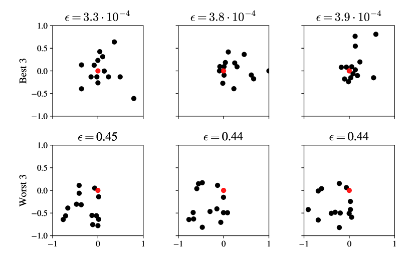
Figure 1: The best 3 stencils with $s=15$ in the top row and the worst 3 in the bottom. The red point marks the central node where we approximate the operator. Positions are centred and normalised.

We generate $10^{5}$ stencils and corresponding labels for sizes of $s\in\{6,7,9,12,15\}$ and combine them into a mixed size dataset that will be denoted as ”mix”. Then, we generate additional $5\cdot 10^{5}$ stencils for sizes of $s\in\{9,15\}$ as single-sized stencil datasets. The automatically generated dataset allows us to extend the size of the dataset in future work as far as required within the computational and time constraints. Creating larger datasets might be beneficial because choosing even the best among $5\cdot 10^{5}$ nodes, as shown in Fig. 1, does not yield even close to perfect stencils.

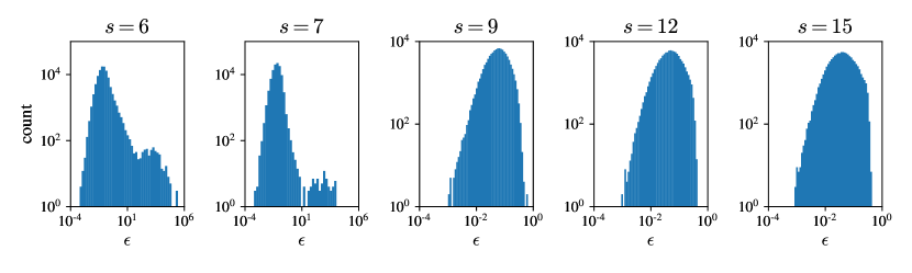
Figure 2: Distribution of error measure $\epsilon$ in datasets for stencils with different sizes $s$. The smaller stencils have a much higher variation.

The distributions of resulting $\epsilon$ labels for different stencil size datasets are shown in Fig. 2. The distributions on the left figures for $s=6$ and $s=7$ provide an additional motivation for this endeavour. Small stencil size is preferred for meshless approximation due to the inherently lower computational costs that are a function of $s$ at every operator evaluation. As this graph shows, small stencils exhibit a much higher variance in quality when compared to their larger counterparts. That makes them less stable and harder to construct when not aided by advanced algorithms.

We discretise the continuous error label into 4 quartiles with equal number of stencils that guarantee a balanced dataset. Some care needs to be taken when determining classes for the ”mix” dataset to maintain consistency. Quartile borders have to be created separately for each of the constituent stencil sizes to account for the different ranges of error labels seen in Fig. 2.

II-A Stencil generation

Random stencil selection needs to be designed in a way that replicates the stencils that are likely to appear in actual use. Purely random node placement is unsuitable due to the possibility of extremely close nodes that would cause instabilities for the approximation. This is established knowledge in the field [7] and the availability of fast and efficient algorithms for generation of candidate nodes prevents this from occurring in practice. On the other hand, using available algorithms for node placement leads to stencils that are too uniform to provide any insight for machine learning.

We circumvent this problem by using an established meshless node positioning algorithm [7] to generate a dense discretization of candidate nodes. The central node is randomly selected from the candidates. The rest of the stencil is then randomly sampled from the candidate nodes with a slightly radially decreasing probability to encourage some extent of aggregation. All $s$ nodes from this stencil are then alternately used as centres when constructing the approximation to introduce more non-symmetric stencils into the mix. We are specially interested in non-symmetric stencils as those are commonly found close to the domain boundaries where stencil construction is the most problematic.

This process is repeated until a desired number of stencils is generated. Stencil coordinates are then transformed into a coordinate representation with origin in the central node and normalized with the distance between the central and the farthest node.

II-B Test fields

As mentioned in the beginning of this section, analytically differentiable fields are required as a benchmark for the RBF-FD approximation. The fields need to be diverse enough to provide a satisfactory proxy for fields encountered during the normal PDE solving and still simple enough to implement a general derivative in C++. We use a benchmark that consists of three fields:

• Monomial

  $$f(x,y)=x^{n}y^{m},\qquad n=2,m=3;$$ (2)

• Sinusoidal

  $$f(x,y)=\sin(k_{x}x)\sin(k_{y}y),\qquad k_{x}=2,k_{y}=1;$$ (3)

• Exponential

  $$f(x,y)=e^{-\frac{x^{2}+y^{2}}{2\sigma}},\qquad\sigma=1.$$ (4)

III Method

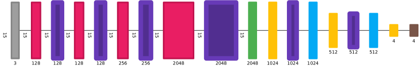
Figure 3: Modified PointNet neural network architecture for $s=15$. Visualisation created directly from the Keras model using the Net2Vis [8] framework.

PointNet[9] was a groundbreaking deep learning algorithm that has opened the field for working with point cloud data. It is mainly used in 3D for classification and segmentation of LiDAR data. The point-based representation offers a much better storage efficiency compared to previously used methods such as voxel grids. The architecture of PointNet is relatively simple. The initial transformations of data lead into a single symmetric max-pooling layer, which is responsible for most of the many beneficial properties that led us to choose this model. In our case, the permutation invariance and the support for internodal interactions were the most important properties.

Initially, we modified the final dense layers of PointNet to work for the task of regression, but the results were underwhelming and comparable to multilayer perceptrons. We settled on discretising our dataset and proceeding with a variation of the standard classification pointNet. The beneficial feature of the max-pooling layer to ignore the contribution of duplicate input coordinates, allowed us to pad the stencil dataset to the same size and utilise the same network for different stencil sizes.

We used a slightly modified version of PointNet with the architecture shown in Fig. 3. The network consists of one-dimensional convolutional layers (Conv1D) with a kernel size of 1 and an increasing number of filters to increase the dimensionality of the input data. The convolutional layers are followed by a max-pooling layer (GlobalMaxPooling1D) that aggregates information from all stencil nodes and constructs a global feature vector used as an input for the dense (Dense) layers. The dense layers utilise dropout (Dropout) layers that randomly drop part of the coefficients and help against over-fitting. The convolutional and the dense layers are augmented with batch normalization and activation layers (NormAct). This version, named vanilla PointNet in the original paper, omits the two transformational layers in the steps before max-pooling. These layers were superfluous based on our testing and only added to the complexity without providing much benefit. This is most likely the case because the stencil data is already translated and well aligned. Instead, we doubled the size of all the other layers. The result is a similar number of weights as in the original network with transformation layers, but with better results in our use-case.

We implemented the modified PointNet in TensorFlow using the Adam optimiser and the sparse categorical crossentrophy loss function. We use ReLu on the intermediate activation layers and softmax on the output. A 0.3 dropout is used with the dense layers. The model was trained with a batch size of 1024 for 20 epochs. The stencil data was split into training and test partitions with 20% intended for testing.

IV Results

The results section focuses on the comparison between the unified mixed stencil size model, implemented by padding smaller stencils, as mentioned in the previous chapter, and three single-size models. All models were trained with identically sized datasets with $5\cdot 10^{5}$ stencils.

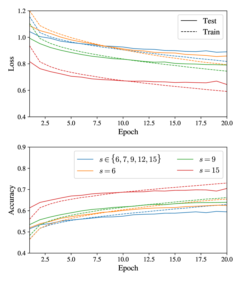
Figure 4: Decrease in loss function and increase in accuracy during the training for three individual stencil sizes and the mix.

First, the training loss and accuracy curves are compared in Fig. 4. The unified model does have slightly worse results, but not drastically so. The accuracy for individual models increases with stencil size. Training is stopped at the arbitrarily selected 20th epoch. A fixed end point is used instead of a stopping criterion based on a validation dataset to ensure a direct comparison between the different models.

We take a closer look at the unified model and its confusion matrix shown in Fig. 5. The columns show what true classes were correctly or incorrectly attributed to the given predicted class. The following discussion shows that the model performs much better than the 60% accuracy would initially suggest. When analysing stencils, we are most interested in the best $Q_{1}$ class of stencils that we definitely want to use and the worst $Q_{4}$ class that we want to avoid at all cost. The classification accuracy is significantly higher for $Q_{1}$ and especially for $Q_{4}$ stencils, which are actually the two classes we are interested in. Additionally, most of the misclassifications for the predicted $Q_{1}$ were actually true $Q_{2}$ and thus still better than the median stencil and vice versa for $Q_{4}$. By definition of equal count quartiles, the stencil with median error falls onto the border between $Q_{2}$ and $Q_{3}$. Its error $\epsilon$ is still relatively small due to the shape of the distributions shown in Figure 2. When accounting for this kind of a misclassification, 92% of stencils classified as $Q_{1}$ were better, and 93% of those classified as $Q_{4}$ were worse than the median stencil.

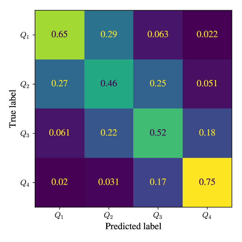
Figure 5: Confusion matrix with normalized columns for the mixed stencil size model with $s\in\{6,7,9,12,15\}$. Values on the diagonal are the correctly identified classes.

We also look at the receiver operating characteristic (ROC) curve in Fig. 6. The model does not return a class directly but a probability that the stencil belongs to any of the classes. The ROC curve plots the true positive rate (TPR) and the false positive rate (FPR) as the threshold probability for classification is varied. A perfect model would be a step function jumping to 1 TPR as soon as the threshold becomes non-zero. We compare how close our models come to this ideal with a metric called area under the curve (AUC) [10] that confirms that our model is particularly good at detecting the bad $Q_{4}$ stencils with a respectable AUC metric of 0.94, and the good $Q_{1}$ stencils with a respectable AUC metric of 0.89.

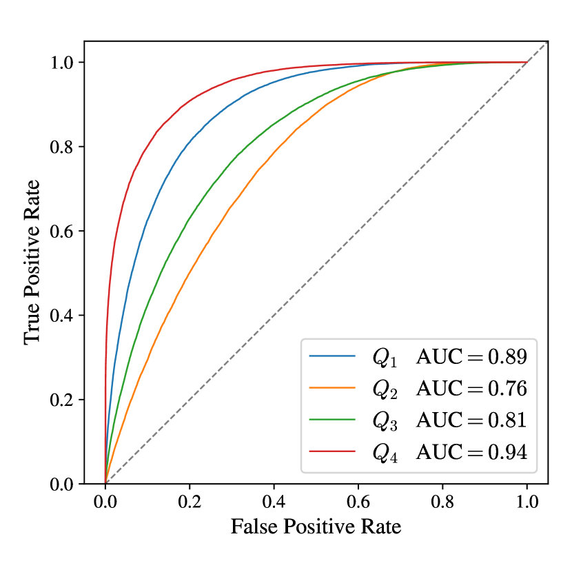
Figure 6: Receiver operating characteristic (ROC) curve for the mixed stencil size model, with the area under the curve (AUC) as one of the classification quality metrics.

The main comparison between mixed and single stencil size models is presented in Table I that holds the extended classification metrics for different variations of test and train datasets. We use four metrics:

• Accuracy is the overall fraction of predictions that were correct;

• Precision is the fraction of the predicted class that was correctly classified;

• Recall is the fraction of the true class that was correctly classified;

• F1 is the harmonic mean of precision and recall;

We notice two trends: (1) the classification results are significantly better for larger stencil sizes; (2) the mixed size model is consistently worse than the dedicated ones, with discrepancy increasing for smaller stencil size. The effect of increasing stencil size is stronger, with $s=15$ classification on the mixed model achieving better overall results than either $s=6$ or $s=9$ on the dedicated models.

The extreme classes remain favoured in classification accuracy but there is a reversal for the small $s=6$ stencil. The best $Q_{1}$ is the most accurately classified class for this dataset achieving the best $Q_{1}$ precision among all the test cases. This could again be explained by the large range of error labels in Fig. 2 making the best quartile more distinct. This is encouraging because the small stencils, as mentioned previously, offer the biggest promise for direct application of this methodology.

The mixed size model provides consistently worse results than the dedicated models and involves additional frivolous computation when padding is required. But still, even with all of the aforementioned caveats, we consider it to be beneficial as it simplifies the stencil building procedure by streamlining the comparison of quality with and without a specific node.

TABLE I: Comparison of metrics between the single and multi-size training

Test	Train	Quartile	Precision	Recall	$F1$	Accuracy
mix	mix	$Q_{1}$	$0.65$	$0.66$	$0.65$	$0.60$
		$Q_{2}$	$0.46$	$0.41$	$0.43$
		$Q_{3}$	$0.52$	$0.55$	$0.54$
		$Q_{4}$	$0.75$	$0.78$	$0.76$
$6$	mix	$Q_{1}$	$0.70$	$0.64$	$0.67$	$0.56$
		$Q_{2}$	$0.47$	$0.46$	$0.46$
		$Q_{3}$	$0.50$	$0.41$	$0.45$
		$Q_{4}$	$0.56$	$0.71$	$0.63$
$6$	$6$	$Q_{1}$	$0.76$	$0.72$	$0.74$	$0.64$
		$Q_{2}$	$0.55$	$0.52$	$0.53$
		$Q_{3}$	$0.57$	$0.55$	$0.56$
		$Q_{4}$	$0.66$	$0.77$	$0.71$
$9$	mix	$Q_{1}$	$0.66$	$0.67$	$0.67$	$0.61$
		$Q_{2}$	$0.49$	$0.41$	$0.44$
		$Q_{3}$	$0.52$	$0.57$	$0.54$
		$Q_{4}$	$0.77$	$0.79$	$0.79$
$9$	$9$	$Q_{1}$	$0.66$	$0.76$	$0.71$	$0.64$
		$Q_{2}$	$0.51$	$0.42$	$0.46$
		$Q_{3}$	$0.55$	$0.57$	$0.56$
		$Q_{4}$	$0.82$	$0.81$	$0.81$
$15$	mix	$Q_{1}$	$0.63$	$0.74$	$0.68$	$0.67$
		$Q_{2}$	$0.50$	$0.40$	$0.44$
		$Q_{3}$	$0.63$	$0.69$	$0.66$
		$Q_{4}$	$0.91$	$0.85$	$0.88$
$15$	$15$	$Q_{1}$	$0.67$	$0.77$	$0.72$	$0.70$
		$Q_{2}$	$0.54$	$0.51$	$0.52$
		$Q_{3}$	$0.68$	$0.66$	$0.67$
		$Q_{4}$	$0.92$	$0.85$	$0.88$

Finally, the confusion matrix for the best model for $s=15$ is shown in Fig. 7. The results are very good and could be used in practice with 97% of nodes classified as $Q_{1}$ below the median stencil error of $\epsilon=3.9\cdot 10^{-2}$ and practically 100% of those classified as $Q_{4}$ above it.

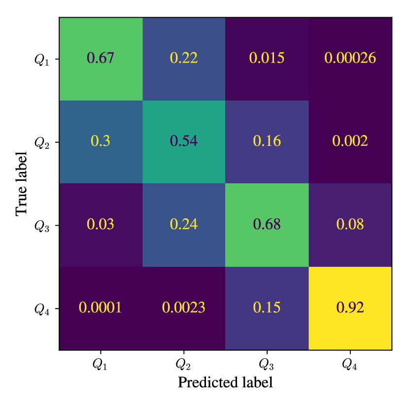
Figure 7: Confusion matrix with normalized columns for the best single stencil size model with $s=15$. Values on the diagonal are the correctly identified classes.

V Future work

This is still a relatively untouched problem, so there is a plethora of future work remaining. We need to incorporate the machine learning based stencil evaluation into a node positioning algorithm and verify that the model can be used to improve the solution procedure and results on a benchmark PDE case. Additionally, steps should be taken to improve the model itself.

The first step would be to improve upon this work and achieve higher classification accuracies by utilising newer and more advanced models [11], as the current results leave much to be desired if we were to use this classifier in practical stencil construction. Furthermore, for direct comparison between differently sized stencils, it would be beneficial if regression replaced classification, as we initially set out to do when starting this work, but neither attempts with multi layer perceptrons nor regressive modification for pointNet returned satisfactory results. Further work is required to determine whether regression would be feasible with the mentioned algorithms or if an alternative approach is required.

The second and probably larger task is to depart from deep learning towards something more explainable that could help us with deeper understanding of the many interconnected factors that contribute to a good stencil. This approach would require some work with feature engineering, but we believe that the benefits would be threefold: faster algorithm, better explainability and higher accuracy.

VI Conclusions

We have presented a methodology for computational generation of labelled stencil datasets that can be used for further data mining endeavours in stencil quality estimation. We have used the pointNet deep learning network to classify the quality of stencils, showing that it performs satisfactory as a proof of concept, but further work would be required before such classifier could be used to build new stencils. The most encouraging aspect of this approach is that the pointNet architecture allows for input padding without a negative impact on the results and thus allows us to use the same network for multiple stencil sizes with worse, but not drastically so, results. This could prove to be very beneficial as it avoids the necessity of having a dedicated network for each stencil size and could allow for cross-size optimisation.

References

- [1] G. R. Liu and Y. T. Gu, An Introduction to Meshfree Methods and Their Programming, 1st ed. Springer Publishing Company, Incorporated, 2010.
- [2] A. I. Tolstykh and D. A. Shirobokov, “On using radial basis functions in a “finite difference mode” with applications to elasticity problems,” Computational Mechanics, vol. 33, no. 1, pp. 68–79, 2003.
- [3] B. Seibold, “Minimal positive stencils in meshfree finite difference methods for the poisson equation,” Computer Methods in Applied Mechanics and Engineering, vol. 198, no. 3, pp. 592–601, 2008. [Online]. Available: https://www.sciencedirect.com/science/article/pii/S0045782508003198
- [4] O. Davydov, D. T. Oanh, and N. M. Tuong, “Improved stencil selection for meshless finite difference methods in 3d,” 2022.
- [5] M. Jančič, J. Slak, and G. Kosec, “Monomial augmentation guidelines for rbf-fd from accuracy versus computational time perspective,” Journal of Scientific Computing, vol. 87, no. 1, p. 9, Feb 2021.
- [6] J. Slak and G. Kosec, “Medusa: A c++ library for solving pdes using strong form mesh-free methods,” ACM Trans. Math. Softw., vol. 47, no. 3, Jun. 2021.
- [7] ——, “On generation of node distributions for meshless PDE discretizations,” SIAM Journal on Scientific Computing, vol. 41, no. 5, pp. A3202–A3229, Oct. 2019.
- [8] A. Bäuerle, C. van Onzenoodt, and T. Ropinski, “Net2vis – a visual grammar for automatically generating publication-tailored cnn architecture visualizations,” IEEE Transactions on Visualization and Computer Graphics, vol. 27, no. 6, pp. 2980–2991, 2021.
- [9] R. Charles, H. Su, M. Kaichun, and L. J. Guibas, “Pointnet: Deep learning on point sets for 3d classification and segmentation,” in 2017 IEEE Conference on Computer Vision and Pattern Recognition (CVPR). Los Alamitos, CA, USA: IEEE Computer Society, jul 2017, pp. 77–85. [Online]. Available: https://doi.ieeecomputersociety.org/10.1109/CVPR.2017.16
- [10] A. P. Bradley, “The use of the area under the roc curve in the evaluation of machine learning algorithms,” Pattern Recognition, vol. 30, no. 7, pp. 1145–1159, 1997. [Online]. Available: https://www.sciencedirect.com/science/article/pii/S0031320396001422
- [11] Y. Guo, H. Wang, Q. Hu, H. Liu, L. Liu, and M. Bennamoun, “Deep learning for 3d point clouds: A survey,” IEEE Transactions on Pattern Analysis and Machine Intelligence, vol. 43, no. 12, pp. 4338–4364, 2021.