Date:

Scalar propagator for planar gravitational waves

Rens van Haasteren^⋆ and Tomislav Prokopec^♢

Institute for Theoretical Physics, Spinoza Institute & EMME$\Phi$

Utrecht University, Princetonplein 5, 3584 CC Utrecht, The Netherlands

Abstract

We construct the massive scalar propagator for planar gravitational wave backgrounds propagating on Minkowski space. We represent the propagator in terms of the Bessel’s function of suitably deformed nonlocal distance functions, the deformation being caused by gravitational waves. We calculate the propagator both for nonpolarized, for the plus ($+$) and cross ($\times$) polarized plane waves, as well as for more general planar waves in $D$ spacetime dimensions. The propagator is useful for studying interactions of scalar fields on planar gravitational wave backgrounds in the context of interacting quantum fields, in which renormalization plays a crucial role. As simple applications of the propagator we calculate the one-loop effective action, the scalar mass generated by the scalar self-interaction term and the one-loop energy-momentum tensor, all renormalized by using dimensional regularization and renormalization. While the effective action and scalar mass remain unaffected by gravitational waves, the energy-momentum tensor exhibits flow of energy density in the direction of gravitational waves which grows quadratically with the scalar field mass, gravitational wave amplitude and its frequency.

^⋆ e-mail: renshaas@hotmail.com

^♢ e-mail: T.Prokopec@uu.nl

1 Introduction

In this work we consider how a massive scalar field responds to planar gravitational waves. In order to facilitate such studies, we first construct the Wightman functions and then the Feynman propagator, which is a fundamental building block for any perturbative studies of an interacting scalar field theory. Anticipating dimensional regularization and renormalization generally required for perturbative studies, we construct the propagator in general (complex) $D$ spacetime dimensions.

This work builds on earlier studies [1, 2, 3, 4, 5, 6, 7, 8], which address some aspects of the problem how planar gravitational waves affect scalar fields. However, none of these works attempts to construct two-point functions and the corresponding Feynman propagator for massive scalar field in classical gravitational wave backgrounds, which is the main goal of this work. This propagator is an essential building block for understanding how quantum scalar fields respond to gravitational waves in various perturbative settings, either through self-interactions or through interactions with other matter fields.

Ref. [1] computes the classical cross section, and pays a particular attention to the focusing of geodesics induced by gravitational waves, a very interesting phenomenon which, to our knowledge, has not been further investigated. In Ref. [2] the 2-gravitons-to-2-photons decay rate was computed. Ref. [3] obtained a non-vanishing complex scalar field condensate and a scalar charge current, the former they interpret as a time-dependent, BEH-like mechanism, driven by the gravitational wave background. In Ref. [4] the imprint of gravitational waves on fermions was investigated for the first time, and in particular how the thus-induced changes in the energy density of neutrinos could be observed in cosmological settings. Ref. [5] has demonstrated that quantum entanglement in atomic systems can be affected by passing gravitational waves, thus paving a way for studies of decoherence induced by gravitational wave backgrounds. The authors of Ref. [6] investigate the response of freely-falling and accelerating Unruh-DeWitt detectors in the presence of gravitational waves.

The model. In this work we cosider a real, self-interacting scalar field $\phi(x)$ whose action and lagrangian are,

$$S[\phi]=\int d^{D}x\sqrt{-g}\,{\cal L}_{\phi}\,,\qquad{\cal L}_{\phi}=-\frac{1}{2}(\partial_{\mu}\phi)(\partial_{\nu}\phi)g^{\mu\nu}-\frac{m^{2}}{2}\phi^{2}-\frac{\lambda}{4!}\phi^{4}\,,\quad$$ (1.1)

where $g={\rm det}[g_{\mu\nu}]$, $g^{\mu\nu}$ is the inverse of the metric tensor $g_{\mu\nu}$, $m$ is the field’s mass and $\lambda$ is the self-interaction coupling strength. We work in natural units in which $c=1$, but keep the dependence on $\hbar$ explicit. This means that the dimension of the field $\phi$ and the mass $m$ is ${\rm m}^{-1}$, and $\lambda$ is dimensionless. To restore the physical dimension of $m$, one ought to rescale it as, $m\rightarrow mc/\hbar$.

1.1 Two representations for gravitational waves

We are interested in understanding the effects of gravitational waves on scalar fields beyond linear order in metric perturbations, so it matters how one represents gravitational wave perturbations. There are two common metric decompositions used in the literature, to which we shall refer to as linear and exponential representation. These representations are not in general equivalent, and that necessitates clarification.

Linear representation. One way of representing a general gravitational wave background is,

$$g_{\mu\nu}(x)=\eta_{\mu\nu}+h_{\mu\nu}(x)\,,$$ (1.2)

where $h_{\mu\nu}(x)$ is a perturbation of the metric tensor $g_{\mu\nu}$ around flat Minkowski space, which is characterised by Minkowski metric $\eta_{\mu\nu}$, which is a $D\times D$ symmetric matrix of the form, $\eta_{\mu\nu}={\rm diag}(-1,1,1,\dots)$.

In the traceless-transverse gauge (in which the gravitational field perturbation $h_{\mu\nu}$ is gauge invariant to linear order in the gravitational field), planar gravitational waves moving in the $x^{D-1}$ direction satisfy $h_{0\mu}=0$ and

$$h_{ij}(x)=h_{ij}^{(0)}\cos\big{[}\omega_{g}t-kx^{D-1}+\psi_{ij}\big{]}\,,\qquad\delta_{ij}h_{ij}(x)=0\,,\qquad\partial_{i}h_{ij}(x)=0\;\;(\forall j)\,,$$ (1.3)

where $\omega_{g}=\|\vec{k}\|\equiv k$ ($c=1$) denotes the gravitational wave frequency, $k$ is its momentum and $h_{ij}^{(0)}$ and $\psi_{ij}\;(i,j,=1,2,\cdots D-1)$ are constant amplitudes and phases, respectively. There are in total $D(D-3)/2$ polarizations. The phases $\psi_{ij}$ are free, but the amplitudes satisfy the conditions, $\delta_{ij}h_{ij}^{(0)}=0$ and $h_{iD-1}^{(0)}=h_{D-1i}^{(0)}=0\;(i=1,2,\cdots,D-1)$. This means that there are $D-3$ linearly independent diagonal polarizations and $(D-2)(D-3)/2$ purely off-diagonal gravitational wave polarizations.

In four spacetime dimensions ($D=4$), a general gravitational wave has two polarizations, known as the plus ($+$) and cross ($\times$) polarizations, and their amplitudes are denoted by $h_{+}$ and $h_{\times}$. A general planar gravitational wave moving in the positive $z-$direction  can be represented as,

$$h_{ij}(x)=h_{+}\epsilon_{ij}^{+}\cos(\omega_{g}u+\psi_{+})+h_{\times}\epsilon_{ij}^{\times}\cos(\omega_{g}u+\psi_{\times})\,,\qquad(u=t-z)\,,$$ (1.4)

where $\psi_{+}$ and $\psi_{\times}$ denote constant phases and $\epsilon_{ij}^{+}$ and $\epsilon_{ij}^{\times}$ are the two polarization tensors,

$$\epsilon_{ij}^{+}=\left(\begin{array}[]{ccc}1&0&0\cr 0&-1&0\cr 0&0&0\cr\end{array}\right)\,,\qquad\epsilon_{ij}^{\times}=\left(\begin{array}[]{ccc}0&1&0\cr 1&0&0\cr 0&0&0\cr\end{array}\right)\,.$$ (1.5)

These gravitational waves have phase velocity, $\vec{v}_{\rm ph}=\hat{z}$, and are often referred to as the positive frequency solutions. In addition there are negative frequency gravitational waves, with an opposite phase velocity ($\vec{v}_{\rm ph}=-\hat{z}$), which are obtained from (1.4) by replacing $\omega_{g}(t-z)$ by $\omega_{g}(t+z)$. If the scalar field is located near a gravitational wave source (such as a binary system), it is a very good approximation to assume that the negative frequency solution is absent, which is what we assume in this paper.

Exponential representation. The spatial metric in this representation for a general gravitational wave propagating in $D$ spacetime dimentions can be written as (cf. Eq. (1.2)),

$$g_{ij}(x)=\left(\!\exp({\mathbf{\tilde{h}}})\right)_{ij}(x)\,,\qquad$$ (1.6)

where $\mathbf{\tilde{h}}$ denotes a $(D-1)\times(D-1)$ symmetric matrix which is traceless and transverse, ${\rm Tr}\!\left[\tilde{h}_{ij}\right]=0$, $\partial_{i}\tilde{h}_{ij}=0$. These two conditions reduce the number of independent components to $D(D-3)/2$. If the gravitational wave is sourced by a binary system in the $xy$ plane, the wave is planar, has two polarizations and propagates in the $x^{D-1}$ direction, then $\tilde{h}_{ij}$ is of the form,

$$\tilde{h}_{ij}\!\! = \!\!\left(\begin{array}[]{cc}\tilde{h}_{+}c_{+}(u)&\tilde{h}_{\times}c_{\times}(u)\cr\tilde{h}_{\times}c_{\times}(u)&-\tilde{h}_{+}c_{+}(u)\cr\end{array}\right)\,,\qquad(i,j=1,2)\,;$$ (1.9)

$$\tilde{h}_{ij}\!\! = \!\!\delta_{ij}\,,\qquad(i,j=3,\cdots D\!-\!2)\,;$$

$$\tilde{h}_{ij}\!\! = \!\!0\,,\qquad\big{(}i=D-1,j=1,\cdots,D\!-\!1\,\wedge\,i=1,\cdots,D\!-\!1,j=D\!-\!1$$ (1.10)

$$\!\!\hskip 42.67912pt\,\wedge\,i=1,2,j=3,\cdots,D\!-\!1\,\wedge\,i=3,\cdots,D\!-\!1,j=1,2\big{)}\,,$$

with $u=t-x^{D-1}$, where $x^{D-1}$ is the direction of propagation,

$$c_{+}(u)=\cos(\omega_{g}u+\psi_{+})\,,\qquad c_{\times}(u)=\cos(\omega_{g}u+\psi_{\times})\,,\qquad$$ (1.11)

$\psi_{+}$ and $\psi_{\times}$ are phases and

$$\tilde{h}(u)=\sqrt{\tilde{h}_{+}^{2}c_{+}^{2}(u)+\tilde{h}_{\times}^{2}c_{\times}^{2}(u)}\,.\qquad$$ (1.12)

Eq. (1.6) can be brought to the form,

$$g_{ij}(u)\!\! = \!\!\left(\begin{array}[]{cc}\cosh[\tilde{h}(u)]+\frac{\sinh[\tilde{h}(u)]}{\tilde{h}(u)}\tilde{h}_{+}c_{+}(u)&\frac{\sinh[\tilde{h}(u)]}{\tilde{h}(u)}\tilde{h}_{\times}c_{\times}(u)\cr\frac{\sinh[\tilde{h}(u)]}{\tilde{h}(u)}\tilde{h}_{\times}c_{\times}(u)&\cosh[\tilde{h}(u)]-\frac{\sinh[\tilde{h}(u)]}{\tilde{h}(u)}\tilde{h}_{+}c_{+}(u)\cr\end{array}\right)\,,\qquad(i,j=1,2)\,;$$ (1.15)

$$g_{ij}\!\! = \!\!\delta_{ij}\,,\qquad(i,j=3,\cdots D\!-\!2)\,;$$

$$g_{ij}\!\! = \!\!0\,,\qquad\big{(}i=D-1,j=1,\cdots,D\!-\!1\,\wedge\,i=1,\cdots,D\!-\!1,j=D\!-\!1$$ (1.16)

$$\!\!\hskip 42.67912pt\,\wedge\,i=1,2,j=3,\cdots,D\!-\!1\,\wedge\,i=3,\cdots,D\!-\!1,j=1,2\big{)}\,.$$

From this form one immediately sees that exponential representation is unimodular, ${\rm det}[g_{ij}]=1$, which makes this representation particularly convenient. Namely, linear representation (1.2) is not unimodular, as ${\rm det}[g_{ij}]\equiv\gamma(u)=1-h_{+}^{2}c_{+}(u)^{2}-h_{\times}^{2}c_{\times}(u)^{2}$, implying that, at higher orders in $h_{ij}$, this representation carries in it spatial, wave-like, scalar gravitational potentials. To see this more clearly, in what follows we construct explicit transformations that relate the two representations. For simplicity we shall do that for $D=4$ and two polarizations, and leave as an exercise to the reader to generalize it to the $D$ dimensional case. To make the mapping possible, we need to modify Eqs. (1.2) and (1.4) by adding two spatial scalar gravitational potentials, namely $\psi_{G}(u)$ and $\zeta_{G}(u)$ of the form,

$$g_{ij}=\delta_{ij}(1+2\psi_{G})+\left(\frac{1}{3}\nabla^{2}\delta_{ij}-\partial_{i}\partial_{j}\right)\zeta_{G}+h_{ij}\,,\quad h_{ij}(u)\!\! = \!\!\left(\begin{array}[]{ccc}h_{+}c_{+}(u)&h_{\times}c_{\times}(u)&0\cr h_{\times}c_{\times}(u)&-h_{+}c_{+}(u)&0\cr 0&0&0\cr\end{array}\right)\,.\qquad$$ (1.20)

Comparing with Eq. (1.16) we see that,

$$h_{+}c_{+}(u)\!\! = \!\!\frac{\sinh[\tilde{h}(u)]}{\tilde{h}(u)}\tilde{h}_{+}c_{+}(u)\,,\qquad h_{\times}c_{\times}(u)=\frac{\sinh[\tilde{h}(u)]}{\tilde{h}(u)}\tilde{h}_{\times}c_{\times}(u)\,,$$

$$\psi_{G}(u)\!\! = \!\!\frac{1}{3}\partial_{z}^{2}\zeta_{G}(u)=\frac{1}{3}\left[\cosh(\tilde{h}(u))-1\right]=\frac{1}{3}\left[\sqrt{1+h(u)^{2}}-1\right]\,,$$ (1.21)

maps exponential representatation $\exp(\tilde{\mathbf{h}})$ onto linear representation, where we have introduced, $h(u)\equiv\sqrt{h_{+}^{2}c_{+}(u)^{2}+h_{\times}^{2}c_{\times}(u)^{2}}$. Conversely we have,

$$\tilde{h}_{+}c_{+}(u)\!\! = \!\!\frac{\ln\left[h(u)+\sqrt{1+h(u)^{2}}\,\right]}{h(u)}h_{+}c_{+}(u)\,,\qquad\tilde{h}_{\times}c_{\times}(u)=\frac{\ln\left[h(u)+\sqrt{1+h(u)^{2}}\,\right]}{h(u)}h_{\times}c_{\times}(u)\,,\qquad$$ (1.22)

where we have used, $h(u)=\sinh\!\left[\tilde{h}(u)\right]$ and $\tilde{h}(u)=\ln\left[h(u)+\sqrt{1+h(u)^{2}}\,\right]$. Since there are no gravitational scalars in exponential representation,  we shall also refer to it as pure tensorial representation.

Now, from the $S$-matrix theory we know that any two metric representations yield equivalent results of physical measurements as long as we know how to map one onto the other, i.e. we know the maps (1.21–1.22). In this paper we shall use both representations, however we point out that exponential representation is advantageous, as it is an unimodular, purely tensorial representation, meaning that it does not carry in it any spatial gravitational potential $\psi_{G}$, which is responsible for local volume deformations, ${\rm det}[\delta_{ij}(1+2\psi_{G})]=(1+2\psi_{G})^{3}$. At a first glance one may surmise that such local volume deformations are not permissible by Birkhoff’s theorem, which states that any spherically symmetric matter configuration cannot source time dependent (propagating) scalar metric perturbations such as $\psi_{G}$. However, planar binary systems which source gravitational waves are not sperically symmetric matter configurations, so Birkhoff’s theorem is not directly applicable. On a deeper level, general relativity couples to matter so that the total gravitational and matter energy is conserved, and the same holds for the energy flow. The local expression of these conservation laws are the $00$ and $0i$ Einstein’s equations, which are known to be non-dynamical. Since gravitational waves carry energy, passage of a gravitational wave can induce a change of the spatial volume in the plane of the wave, making such local volume deformations travelling with the speed of light physically justified. The transversal nature of gravitational waves should prevent spatial deformations in the direction of propagation however, thus favouring exponential representation. For the sake of comparison and for completeness, in this paper we shall consider both linear and exponential representation, but we will pay a special attention when making statements concerning the physical effects on matter fields induced at higher orders in metric perturbations by passing gravitational waves.

In what follows, we consider canonical quantization in Cartesian and lightcone coordinates. Lightcone coordinates are convenient as the Klein-Gordon equation obeyed by the scalar field simplifies in these coordinates. However, canonical quantization in lightcone coordinates is quite subtle, and for that reason we devote the whole section 2 to review it. For readers familiar with lightcone quantization, we suggest to go directly to section 3.

2 Quantization in lightcone coordinates

To emphasise the differences and similarities between quantization in Cartesian and lightcone coordinates, in this section we describe both quantizations. Anticipating the use of dimensional regularization, we perform quantization in $D$ spacetime dimensions, and then discuss the reduction to $4$ spacetime dimensions.

We begin by recalling coordinate independent generalities of canonical quantization. The scalar field action (1.1) implies canonical momentum, $\Pi(x)=\delta S/\delta\partial_{0}\phi(x)=-\sqrt{-g}g^{0\mu}\partial_{\mu}\phi(x)$, where the subscript $0$ refers to the time coordinate, which must be non-spacelike. Canonical quantization then promotes $\phi$ and $\Pi$ into operators which satisfy a canonical quantization commutator,

$$\big{[}\hat{\phi}(x^{0},\vec{x}),\hat{\Pi}(x^{0},\vec{x}^{\,\prime})\big{]}=i\hbar\delta^{D-1}(\vec{x}-\vec{x}\,^{\prime})\,.$$ (2.1)

The Feynman propagator equation can be written on a general gravitational background as,

$$\big{(}\Box-m^{2}\big{)}i\Delta_{F}(x;x^{\prime})=i\hbar\frac{\delta^{D}(x-x^{\prime})}{\sqrt{-g}}\,,$$ (2.2)

where the d’Alembertian operator $\Box$ acts on a scalar as,

$$\Box=\frac{1}{\sqrt{-g}}\partial_{\mu}{\sqrt{-g}}g^{\mu\nu}\partial_{\nu}\,,$$ (2.3)

and the quantum field $\hat{\phi}(x)$ satisfies a Klein-Gordon equation,

$$(\Box-m^{2})\hat{\phi}(x)=0\,.$$ (2.4)

In equation (2.2) both the d’Alembertian operator and the Dirac delta function are (bi-)scalars under general coordinate transformations, implying that one can seek the propagator solution to be a biscalar (i.e. scalar on both legs: $x$ and $x^{\prime}$). One can assume the propagator solution to be of the form,

$$i\Delta_{F}(x;x^{\prime})=\Theta(\Delta x^{0})i\Delta^{(+)}(x;x^{\prime})+\Theta(-\Delta x^{0})i\Delta^{(-)}(x;x^{\prime})\,,$$ (2.5)

where $\Theta(x)$ denotes the Heaviside theta function, $\Delta x^{0}=x^{0}\!-\!x^{0\,\prime}$ and $i\Delta^{(+)}(x;x^{\prime})$ and $i\Delta^{(-)}(x;x^{\prime})$ are homogeneous solutions known as the positive and negative frequency Wightman functions, respectively, satisfying,

$$\big{(}\Box-m^{2}\big{)}i\Delta^{(\pm)}(x;x^{\prime})=0\,.$$ (2.6)

For a given state $|\Omega\rangle$, the Wightman functions can be written as the following two-point functions,

$$i\Delta^{(+)}(x;x^{\prime})=\langle\Omega|\hat{\phi}(x)\hat{\phi}(x^{\prime})|\Omega\rangle\,,\qquad i\Delta^{(+)}(x;x^{\prime})=\langle\Omega|\hat{\phi}(x^{\prime})\hat{\phi}(x)|\Omega\rangle\,,$$ (2.7)

which – in the absence of interactions – clearly satisfy (2.6). It is important to notice that the propagator equation (2.2) is consistent with canonical quantization (2.1). Indeed, upon inserting (2.5) into (2.2) one obtains that one time derivative $\partial_{0}$ from $\Box$ commutes through Heaviside functions  in (2.5) and hits the field $\hat{\phi}(x)$ creating a canonical momentum term, and the other produces Dirac’s delta functions according to, $\partial_{0}\Theta(\Delta x^{0})=\delta(\Delta x^{0})=-\partial_{0}\Theta(-\Delta x^{0})$, resulting in,

$$\big{(}\Box-m^{2}\big{)}i\Delta_{F}(x;x^{\prime})=-\frac{1}{\sqrt{-g}}\delta(\Delta x^{0})\langle\Omega|\big{[}\hat{\Pi}(x),\hat{\phi}(x^{\prime})\big{]}\Omega\rangle=\frac{1}{\sqrt{-g}}i\hbar\delta(x^{0}\!-\!x^{0\,\prime})\delta^{D-1}(\vec{x}\!-\!\vec{x}^{\,\prime})\,,$$ (2.8)

which equals the right-hand-side of (2.2). Since this is true in any coordinate system,  this procedure should allow one to fix canonical quantization in any coordinates.

2.1 Quantization in Cartesian coordinates

We now proceed with canonical quantization in Cartesian coordinates in Minkowski space,  in which $\Box\rightarrow\partial^{2}=\eta^{\mu\nu}\partial_{\mu}\partial_{\nu}$, by rewriting the operators $\hat{\phi}(x)$ and $\hat{\Pi}(x)$ in terms of the momentum space mode operators as,

$$\hat{\phi}(x)=\int\!\frac{{\rm d}^{D}k}{(2\pi)^{D}}{\rm e}^{ik\cdot x}\hat{\phi}(k^{\alpha})\,,\quad\hat{\Pi}(x)=\int\!\frac{{\rm d}^{D}k}{(2\pi)^{D}}{\rm e}^{ik\cdot x}\hat{\Pi}(k^{\alpha})\,,\quad\big{(}k\cdot x=\eta_{\mu\nu}k^{\mu}x^{\nu}=-k^{0}x^{0}+\vec{k}\cdot\vec{x}\big{)}\,.\qquad$$ (2.9)

The mode operators obey algebraic equations, which follow from the Klein-Gordon equation (2.4),

$$\big{[}\!(k^{0})^{2}-\omega^{2}\big{]}\hat{\phi}(k^{\alpha})=0,\quad\big{[}\!(k^{0})^{2}-\omega^{2}\big{]}\hat{\Pi}(k^{\alpha})=0\,,\quad\omega^{2}=\|\vec{k}\|^{2}+m^{2}\,,\qquad$$ (2.10)

whose general solutions can be written as,

$$\hat{\phi}(k^{\alpha})=\hat{\phi}_{+}(\vec{k})2\pi\delta(k^{0}-\omega)+\hat{\phi}_{-}(\vec{k})2\pi\delta(k^{0}+\omega)\,,\quad\hat{\Pi}(k^{\alpha})=\hat{\Pi}_{+}(\vec{k})2\pi\delta(k^{0}-\omega)+\hat{\Pi}_{-}(\vec{k})2\pi\delta(k^{0}+\omega)\,,$$ (2.11)

where $\omega$ denotes the quasiparticle frequency and $\hat{\phi}_{+}(\vec{k})$ and $\hat{\phi}_{-}(\vec{k})$ are the positive and negative frequency mode operators, respectively. Upon inserting (2.11) into (2.9) and integrating over $k^{0}$ one obtains,

$$\hat{\phi}(x)=\int\!\frac{{\rm d}^{D-1}k}{(2\pi)^{D-1}}{\rm e}^{i\vec{k}\cdot\vec{x}}\big{[}{\rm e}^{-i\omega t}\hat{\phi}_{+}(\vec{k})+{\rm e}^{-i\omega t}\hat{\phi}_{-}(\vec{k})\big{]}\,,\quad\hat{\Pi}(x)=\int\!\frac{{\rm d}^{D-1}k}{(2\pi)^{D-1}}{\rm e}^{i\vec{k}\cdot\vec{x}}\big{[}{\rm e}^{-i\omega t}\hat{\Pi}_{+}(\vec{k})+{\rm e}^{-i\omega t}\hat{\Pi}_{-}(\vec{k})\big{]}\,.\quad$$ (2.12)

The hermiticity conditions, $\hat{\phi}^{\dagger}(x)=\hat{\phi}(x)$ and $\hat{\Pi}^{\dagger}(x)=\hat{\Pi}(x)$ impose on the mode operators,

$$\left[\hat{\phi}_{+}(\vec{k})\right]^{\dagger}=\hat{\phi}_{-}(-\vec{k})\,,\qquad\left[\hat{\Pi}_{+}(\vec{k})\right]^{\dagger}=\hat{\Pi}_{-}(-\vec{k})\,,$$ (2.13)

which ensure that the momentum transformation (2.12) preserves the number of (on-shell) degrees of freedom. This implies that, for a real scalar field, the positive and negative frequency poles do not fluctuate independently. The mode operators obey canonical quantization relations,

$$\big{[}\hat{\phi}_{+}(\vec{k}),\hat{\Pi}_{-}(\vec{k}^{\prime})\big{]}=\frac{i\hbar}{2}(2\pi)^{D-1}\delta^{D-1}(\vec{k}+\vec{k}^{\prime})=\big{[}\hat{\phi}_{-}(\vec{k}),\hat{\Pi}_{+}(\vec{k}^{\prime})\big{]}\,,$$ (2.14)

and the other two vanish, $\big{[}\hat{\phi}_{+}(\vec{k}),\hat{\Pi}_{+}(\vec{k}^{\prime})\big{]}=0=\big{[}\hat{\phi}_{-}(\vec{k}),\hat{\Pi}_{-}(\vec{k}^{\prime})\big{]}$. One can now easily check that inserting (2.12) into $\big{[}\hat{\phi}(x^{0},\vec{x}),\hat{\Pi}(x^{0},\vec{x}^{\,\prime})\big{]}$ and making use of (2.14) reproduces the canonical quantization relation (2.1). As a consequence of the hermiticity condition in (2.13) the two commutators in (2.14) must be equal, which physically means that the vacuum fluctations on the positive and negative frequency poles are of an equal strength.

Next, taking account of $\hat{\Pi}(x)=\partial_{t}\hat{\phi}(x)$ implies, $\hat{\Pi}_{\pm}(\vec{k})=\mp i\omega\hat{\phi}_{\pm}(\vec{k})$, from which the more common annihilation and creation representation of the mode operators follows,

$$\hat{\phi}_{+}(\vec{k})=\sqrt{\frac{\hbar}{2\omega}}\hat{a}(\vec{k})\,,\quad\hat{\phi}_{-}(\vec{k})=\sqrt{\frac{\hbar}{2\omega}}\hat{a}^{\dagger}(-\vec{k})\,,\qquad\hat{\Pi}_{+}(\vec{k})=-i\sqrt{\frac{\hbar\omega}{2}}\hat{a}(\vec{k})\,,\quad\hat{\Pi}_{-}(\vec{k})=i\sqrt{\frac{\hbar\omega}{2}}\hat{a}^{\dagger}(-\vec{k})\,,$$ (2.15)

which obey,

$$\big{[}\hat{a}(\vec{k}),\hat{a}^{\dagger}(\vec{k}^{\prime})\big{]}=(2\pi)^{D-1}\delta^{D-1}(\vec{k}-\vec{k}^{\prime})\,;\quad\big{[}\hat{a}(\vec{k}),\hat{a}(\vec{k}^{\prime})\big{]}=0=\big{[}\hat{a}^{\dagger}(\vec{k}),\hat{a}^{\dagger}(\vec{k}^{\prime})\big{]}\,.$$ (2.16)

The operators $\hat{a}(\vec{k})$ and $\hat{a}^{\dagger}(\vec{k})$ are interpreted as the operators that annihilate the vacuum state $|\Omega\rangle$,

$$\hat{a}(\vec{k})|\Omega\rangle=0\,,$$ (2.17)

and create a particle of momentum $\vec{k}$, $\hat{a}^{\dagger}(\vec{k})|\Omega\rangle=|1_{\vec{k}}\rangle$, respectively. Notice that, as a consequence of the hermiticity conditions (2.13), the two commutators in (2.14) collapse into one (nontrivial) commutator (2.16).

         

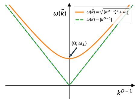
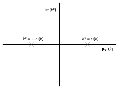
Figure 1: Left panel: Frequency versus $k^{D-1}$ for Cartesian coordinates. Right panel: The quasiparticle poles $k^{0}=\pm\omega$ in the complex $k^{0}-$plane. The poles are symmetric with respect to ${\Re}[k^{0}]=0$.

Clearly, if $\hat{a}(\vec{k})$ annihilate the vacuum, so do $\hat{\phi}_{+}(\vec{k})$. One can construct a more general (pure, Gaussian) state by relaxing that condition. In this case one can write,

$$\hat{\phi}_{+}(\vec{k})=\sqrt{\frac{\hbar}{2\omega}}\big{[}\alpha(\vec{k})\hat{a}(\vec{k})+\beta^{*}(-\vec{k})\hat{a}^{\dagger}(-\vec{k})\big{]}\,,\quad\hat{\phi}_{-}(\vec{k})=\sqrt{\frac{\hbar}{2\omega}}\big{[}\beta(\vec{k})\hat{a}(\vec{k})+\alpha^{*}(-\vec{k})\hat{a}^{\dagger}(-\vec{k})\big{]}\,,$$ (2.18)

where the form of the second relation is determined by the hermiticity condition (2.13), and – provided $|\alpha(\vec{k})|^{2}-|\beta(\vec{k})|^{2}=1$ – canonical quantization (2.1) remains satisfied. The state (2.18) is the most general pure Gaussian state, and it corresponds to an excited state, in the sense that its energy per mode is enhanced by a factor $|\alpha(\vec{k})|^{2}+|\beta(\vec{k})|^{2}>1$ when compared with the energy per mode of the vacuum state (2.15).

The final remark we make is that (as a consequence of the CPT theorem), the positive and negative frequency poles, $k^{0}=\pm\omega$, are symmetrically distributed around the origin in the complex $k^{0}-$plane, which is illustrated in figure 1. In what follows, we show that quantization in lightcone coordinates yields a surprising result with regard to the distribution of the positive and negative frequency poles.

2.2 Quantization in lightcone coordinates

We begin this section by an important observation regarding canonical quantization in lightcone coordinates. The Feynman propagator in lightcone coordinates is defined as,

$$i\Delta_{F}(x;x^{\prime})=\Theta(\Delta u)i\Delta^{(+)}(x;x^{\prime})+\Theta(-\Delta u)i\Delta^{(-)}(x;x^{\prime})\,.$$ (2.19)

Inserting this into Eq. (2.2) one obtains that canonical quantization in lightcone coordinates ought to change to,

$$[\hat{\phi}(u,\vec{x}_{\perp},v),\hat{\Pi}(u,\vec{x}_{\perp}^{\,\prime},v^{\prime})]=\frac{i}{2}\hbar\delta^{D-2}(\vec{x}_{\perp}-\vec{x}_{\perp}^{\,\prime})\delta(v-v^{\prime})\,$$ (2.20)

to make it consistent with the covariant propagator equation (2.2), which should take preponderance  over canonical quantization as it is written in a coordinate independent way and therefore should hold in any coordinates. The question is what went wrong in the proof of consistency between canonical quantization (2.1) and the propagator equation (2.2). The principal mistake in the ‘proof’ was the assumption that the d’Alembertian operator has two time derivatives, of which one commutes through the $\Theta$-functions on the account of a vanishing Jordan two-point function on spatial separations. Firstly, in the d’Alembertian operator in lightcone coordinates there is only one time coordinate $\partial_{u}$, and therefore it must hit the $\Theta$-functions to produce the needed Dirac $\delta$-function, $\delta(\Delta u)$. Secondly, equal time Jordan function needs not to vanish (and does not vanish!) at equal time ($u^{\prime}=u$) hypersurfaces, because these hypersurfaces are lightlike, not spacelike. Indeed, the equal time Jordan function exhibits correlations of the type,

$$\left\langle\Omega\right|\left[\hat{\phi}(u,\vec{x}_{\perp},v),\hat{\phi}(u,\vec{x}_{\perp}^{\,\prime},v^{\prime})\right]\left|\Omega\right\rangle=\frac{i\hbar}{2}\delta^{D-2}(\vec{x}_{\perp}-\vec{x}_{\perp}^{\,\prime})\frac{1}{2}{\rm sign}(v-v^{\prime})\,.$$ (2.21)

The factor $1/2$ in (2.20) arises simply because the derivative $\partial_{u}$ appears twice in the d’Alembertian in lightcone coordinates,

$$\Box=\frac{1}{\sqrt{-g}}\left[\partial_{u}\sqrt{-g}g^{uv}\partial_{v}+\partial_{v}\sqrt{-g}g^{vu}\partial_{u}+\cdots\right]\,,$$ (2.22)

thus generating two times the canonical commutator of $\hat{\phi}$ and $\hat{\Pi}$.

We are now ready to study vacuum fluctuations in lightcone coordinates (2.23). In what follows we repeat the analysis of section 2.1, thereby emphasising the particularities of lightcone quantization.

From the Minkowski metric in Cartesian coordinates, in which $\eta_{\mu\nu}$ is a diagonal $D\times D$ matrix of the form, $\eta_{\mu\nu}={\rm diag}(-1,1,1,\cdots,1)$ and coordinate transformations,

$$u=t-x^{D-1}\,,\qquad v=t+x^{D-1}\,,\qquad\vec{x}_{\perp}=\vec{x}_{\perp}\,,$$ (2.23)

one obtains the metric in lightcone coordinates and its inverse in the form,

$$g_{uv}\!\! = \!\!g_{vu}=-\frac{1}{2}\,,\qquad g_{ij}=\delta_{ij}\;\;(i,j=1,2,\cdots,D\!-\!2)\,,$$ (2.24)

$$g^{uv}\!\! = \!\!g^{vu}=-2\,,\qquad g^{ij}=\delta_{ij}\;\;(i,j=1,2,\cdots,D\!-\!2)\,,$$ (2.25)

such that ${\rm det}[g_{\mu\nu}]=-1/4$. 

Performing the same type of Fourier transformation as in (2.9), where now the invariant phase is 

$$k\cdot x=\vec{k}_{\perp}\cdot\vec{x}_{\perp}-\frac{1}{2}(k^{u}v+k^{v}u)\,,$$ (2.26)

one obtains that the Klein-Gordon equation (2.4) reduces to algebraic equations for the mode operators (2.10), which in lightcone coordinates become,

$$\big{(}k^{u}k^{v}-\omega_{\perp}^{2}\big{)}\hat{\phi}(k^{\alpha})=0,\quad\big{(}k^{u}k^{v}-\omega_{\perp}^{2}\big{)}\hat{\Pi}(k^{\alpha})=0\,,\qquad\omega_{\perp}^{2}=\|\vec{k}_{\perp}\|^{2}+m^{2}\,.$$ (2.27)

These equations tell us that, $k^{u}=\omega_{\perp}^{2}/k^{v}$,  and it seems that there is only one frequency pole. That is not true however, since $k^{v}$ can be both positive and negative, and therefore we have two symmetric quasiparticle poles, $k^{u}=\omega_{\perp}^{2}/|k^{v}|$ (when $k^{v}>0$) and $k^{u}=-\omega_{\perp}^{2}/|k^{v}|$ (when $k^{v}<0$). This then implies the following general solution,

$$\hat{\phi}(k^{\alpha})\!\! = \!\!\hat{\phi}_{+}^{\rm LC}(\vec{k}_{\perp},k^{v})2\pi\delta\big{(}k^{u}-\omega_{\perp}^{2}/|k^{v}|\big{)}\Theta(k^{v})+\hat{\phi}_{-}^{\rm LC}(\vec{k}_{\perp},k^{v})2\pi\delta\big{(}k^{u}+\omega_{\perp}^{2}/|k^{v}|\big{)}\Theta(-k^{v})$$

$$\hat{\Pi}(k^{\alpha})\!\! = \!\!\hat{\Pi}_{+}^{\rm LC}(\vec{k}_{\perp},k^{v})2\pi\delta\big{(}k^{u}-\omega_{\perp}^{2}/|k^{v}|\big{)}\Theta(k^{v})+\hat{\Pi}_{-}^{\rm LC}(\vec{k}_{\perp},k^{v})2\pi\delta\big{(}k^{u}+\omega_{\perp}^{2}/|k^{v}|\big{)}\Theta(-k^{v})\,,$$ (2.28)

where we introduced the superscript ${\rm LC}$ to distinguish the mode operators in lightcone coordinates from those in Cartesian coordinates in Eq. (2.12). When these are inserted into (2.9) and integration over $k^{u}$ is performed one obtains,

$$\hat{\phi}(x)\!\! = \!\!\!\int\!\frac{{\rm d}^{D-2}k_{\perp}{\rm d}k^{v}}{(2\pi)^{D-1}}{\rm e}^{i\vec{k}_{\perp}\cdot\vec{x}_{\perp}}\big{[}{\rm e}^{-\frac{i}{2}(k^{v}u+v\omega_{\perp}^{2}/k^{v})}\hat{\phi}_{+}^{\rm LC}(\vec{k}_{\perp},k^{v})\Theta(k^{v})+{\rm e}^{-\frac{i}{2}(k^{v}u+v\omega_{\perp}^{2}/k^{v})}\hat{\phi}_{-}^{\rm LC}(\vec{k}_{\perp},k^{v})\Theta(-k^{v})\big{]}\,,\quad$$

$$\hat{\Pi}(x)\!\! = \!\!\!\int\!\frac{{\rm d}^{D-2}k_{\perp}{\rm d}k^{v}}{(2\pi)^{D-1}}{\rm e}^{i\vec{k}_{\perp}\cdot\vec{x}_{\perp}}\big{[}{\rm e}^{-\frac{i}{2}(k^{v}u+v\omega_{\perp}^{2}/k^{v})}\hat{\Pi}_{+}^{\rm LC}(\vec{k}_{\perp},k^{v})\Theta(k^{v})+{\rm e}^{-\frac{i}{2}(k^{v}u+v\omega_{\perp}^{2}/k^{v})}\hat{\Pi}_{-}^{\rm LC}(\vec{k}_{\perp},k^{v})\Theta(-k^{v})\big{]}.$$

(2.29)

In analogy with canonical quantization in Cartesian coordinates, one can introduce the lightcone vacuum $|\Omega\rangle_{\rm LC}$ defined by,

$$\hat{\phi}_{+}^{\rm LC}(\vec{k}_{\perp},k^{v})|\Omega\rangle_{\rm LC}=0\,.$$ (2.30)

A natural question that arises is: how are the two vacua $|\Omega\rangle_{\rm LC}$ and $|\Omega\rangle\equiv|\Omega\rangle_{\rm Cartesian}$ in Eq. (2.17) related.

To answer this important question, we need to establish the relation between the mode operators $\hat{\phi}_{\pm}^{\rm LC}(\vec{k}_{\perp},k^{v})$, $\hat{\Pi}_{\pm}^{\rm LC}(\vec{k}_{\perp},k^{v})$ in lightcone coordinates in Eqs. (2.29) with those in Cartesian coordinates $\hat{\phi}_{\pm}(\vec{k}_{\perp},k^{v})$, $\hat{\Pi}_{\pm}(\vec{k}_{\perp},k^{v})$ in Eqs. (2.12). Firstly, observe that $k\cdot x$ is a scalar phase, and therefore invariant under coordinate transformations, which implies,

$$\vec{k}_{\perp}\cdot\vec{x}_{\perp}-k^{0}t+k^{D-1}x^{D-1}=\vec{k}_{\perp}\cdot\vec{x}_{\perp}-\frac{1}{2}\big{(}k^{u}v+k^{v}u\big{)}\,,$$ (2.31)

from where one infers,

$$k^{D-1}=\frac{k^{v}\!-\!k^{u}}{2}\,,\quad k^{0}=\frac{k^{v}\!+\!k^{u}}{2}\;\;\Longrightarrow\;\;k^{v}=k^{0}\!+\!k^{D-1}=-2k_{u}\,,\quad k^{u}=k^{0}\!-\!k^{D-1}=-2k_{v}\,.\;$$ (2.32)

Next, by recalling that on the positive frequency shell, $k^{u}=\omega_{\perp}^{2}/k^{v}$ and $k^{0}=\omega$ ($k^{v}>0$), and on the negative frequency shell, $k^{u}=\omega_{\perp}^{2}/k^{v}$ and $k^{0}=-\omega$ ($k^{v}<0$), and upon dropping the trivial contribution $\vec{k}_{\perp}\cdot\vec{x}_{\perp}$ one obtains the following on-shell version of the phase relations (2.31), 

$${\rm Positive\;frequency\;shell:}\qquad-\frac{1}{2}\big{(}\Omega_{-}v+\Omega_{+}u\big{)}\!\! = \!\!-\omega t+k^{D-1}x^{D-1}$$

$${\rm Negative\;frequency\;shell:}\qquad\quad\!\frac{1}{2}\big{(}\Omega_{+}v+\Omega_{-}u\big{)}\!\! = \!\!\omega t+k^{D-1}x^{D-1}\,,$$ (2.33)

where we dropped the trivial parts $\vec{k}_{\perp}\cdot\vec{x}_{\perp}$, and we have introduced shifted frequencies,

$$\Omega_{\pm}(\vec{k})=\omega\pm k^{D-1}\,,$$ (2.34)

such that $\Omega_{\pm}(-\vec{k})=\Omega_{\mp}(\vec{k})$.

         

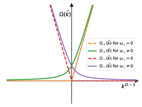
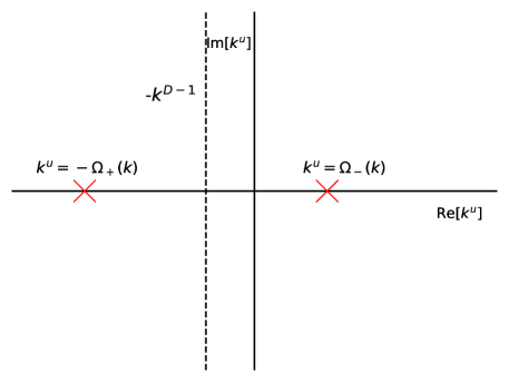
Figure 2: Left panel: Quasiparticle frequencies $\Omega_{\pm}$ versus $k^{D-1}$ for lightcone coordinates for the cases when $\omega_{\perp}\neq 0$ (solid) and when $\omega_{\perp}=0$ (dashed). Right panel: Quasiparticle poles $k^{u}=-2k_{v}=\Omega_{-}=\omega-k^{D-1}$ and $k^{u}=-2k_{v}=-\Omega_{+}=-(\omega+k^{D-1})$ in the complex $k^{u}-$plane. The poles are not symmetric with respect to ${\Re}[k^{u}]=0$, but they are symmetric with respect to ${\Re}[k^{u}]=-k^{D-1}$.

Therefore, when expressed in Cartesian coordinates, the positive and negative frequency poles of lightcone coordinates appear not to be symmetric, as can be seen in figure 2. The next step is to convert the integral measure in (2.29) into Cartesian coordinates to yield,

$$\hat{\phi}(x)\!\! = \!\!\!\int\!\frac{{\rm d}^{D-2}k_{\perp}{\rm d}k^{D-1}}{(2\pi)^{D-1}}{\rm e}^{i\vec{k}_{\perp}\cdot\vec{x}_{\perp}}\bigg{[}{\rm e}^{-\frac{i}{2}(\Omega_{-}v+\Omega_{+}u)}\frac{\Omega_{+}}{\omega}\hat{\phi}_{+}^{\rm LC}(\vec{k}_{\perp},\Omega_{+})+{\rm e}^{\frac{i}{2}(\Omega_{+}v+\Omega_{-}u)}\frac{\Omega_{-}}{\omega}\hat{\phi}_{-}^{\rm LC}(\vec{k}_{\perp},-\Omega_{-})\bigg{]}\,,\quad$$

$$\hat{\Pi}(x)\!\! = \!\!\!\int\!\frac{{\rm d}^{D-2}k_{\perp}{\rm d}k^{D-1}}{(2\pi)^{D-1}}{\rm e}^{i\vec{k}_{\perp}\cdot\vec{x}_{\perp}}\bigg{[}{\rm e}^{-\frac{i}{2}(\Omega_{-}v+\Omega_{+}u)}\frac{\Omega_{+}}{\omega}\hat{\Pi}_{+}^{\rm LC}(\vec{k}_{\perp},\Omega_{+})+{\rm e}^{\frac{i}{2}(\Omega_{+}v+\Omega_{-}u)}\frac{\Omega_{-}}{\omega}\hat{\Pi}_{-}^{\rm LC}(\vec{k}_{\perp},-\Omega_{-})\bigg{]}\,,\qquad\;\;$$ (2.35)

where we made use of, ${\rm d}k^{v}={\rm d}\Omega_{+}=(\Omega_{+}/\omega){\rm d}k^{D-1}$, for the positive frequency shell and of, ${\rm d}k^{v}={\rm d}(-\Omega_{-})=(\Omega_{-}/\omega){\rm d}k^{D-1}$, for the negative frequency shell. Finally, by comparing (2.35) with Eq. (2.12), one obtains the desired relations,

$$\hat{\phi}_{+}(\vec{k})\!\! = \!\!\frac{\Omega_{+}}{\omega}\hat{\phi}_{+}^{\rm LC}(\vec{k}_{\perp},\Omega_{+})=\sqrt{\frac{\hbar}{2\omega}}\hat{a}(\vec{k}\,)\,,\qquad\hat{\phi}_{-}(\vec{k})=\frac{\Omega_{-}}{\omega}\hat{\phi}_{-}^{\rm LC}(\vec{k}_{\perp},-\Omega_{-})=\sqrt{\frac{\hbar}{2\omega}}\hat{a}^{\dagger}(-\vec{k}\,)\,,\qquad$$ (2.36)

$$\hat{\tilde{\Pi}}_{\pm}(\vec{k})\!\! = \!\!\frac{\Omega_{\pm}}{\omega}\hat{\Pi}_{\pm}^{\rm LC}(\vec{k}_{\perp},\pm\Omega_{\pm})\,.$$ (2.37)

The mapping for the momentum operators $\hat{\bar{\Pi}}_{\pm}(\vec{k})$ in (2.37) yields canonical momenta in Cartesian coordinates. However, these momenta correspond to the momenta defined by $\hat{\tilde{\Pi}}=\partial_{t}\hat{\phi}$, and therefore they are not the canonical momenta we need for quantization in lightcone coordinates, in which they are defined as, $\hat{\Pi}=\partial_{v}\hat{\phi}=\frac{1}{2}(\partial_{t}+\partial_{z})\hat{\phi}$. Incorporating this definition changes the relation between the field mode operators and the corresponding canonical momenta in lightcone coordinates from $\hat{\tilde{\Pi}}_{\pm}=\mp i\omega\phi_{\pm}$ to,

$$\hat{\Pi}_{+}(\vec{k})=-\frac{i}{2}\Omega_{-}(\vec{k})\hat{\phi}_{+}(\vec{k})\,,\quad\hat{\Pi}_{-}(\vec{k})=\frac{i}{2}\Omega_{+}(\vec{k})\hat{\phi}_{-}(\vec{k})\,.\quad$$ (2.38)

Relations (2.36) and (2.38) completely define the mapping between the positive and negative frequency mode operators in lightcone coordinates to those in Cartesian coordinates.

Since the mapping does not mix the positive and negative frequency mode operators, the two vacua are identical (cf. Eqs. (2.17) and (2.30)),

$$|\Omega\rangle_{\rm LC}=|\Omega\rangle\,,$$ (2.39)

which answers the principal question we have asked above. The trivial identification of the two vacua in Eq. (2.39) is a consequence of the judicious split into the positive and negative frequency operators in Eq. (2.28–2.29). With these observations in mind, we can write the following convenient on-shell decomposition of the field operators,

$$\hat{\phi}(x)\!\! = \!\!\!\int\!\frac{{\rm d}^{D-1}k}{(2\pi)^{D-1}}{\rm e}^{i\vec{k}_{\perp}\cdot\vec{x}_{\perp}}\Big{[}{\rm e}^{-\frac{i}{2}\Omega_{-}v}\phi_{+}(u,\vec{k}\,)\hat{a}(\vec{k}\,)+{\rm e}^{\frac{i}{2}\Omega_{+}v}\phi_{-}(u,\vec{k}\,)\hat{a}^{\dagger}(-\vec{k}\,)\Big{]}\,,\quad$$ (2.40)

$$\hat{\Pi}(x)\!\! = \!\!\!\int\!\frac{{\rm d}^{D-1}k}{(2\pi)^{D-1}}{\rm e}^{i\vec{k}_{\perp}\cdot\vec{x}_{\perp}}\Big{[}{\rm e}^{-\frac{i}{2}\Omega_{-}v}\Pi_{+}(u,\vec{k}\,)\hat{a}(\vec{k}\,)+{\rm e}^{\frac{i}{2}\Omega_{+}v}\Pi_{-}(u,\vec{k}\,)\hat{a}^{\dagger}(-\vec{k}\,)\Big{]}\,,\qquad\;\;$$ (2.41)

where the vacuum mode functions are,

$$\phi_{+}(u,\vec{k}\,)=\sqrt{\frac{\hbar}{2\omega}}\;{\rm e}^{-\frac{i}{2}\Omega_{+}(\vec{k})u}\,,\quad\phi_{-}(u,\vec{k}\,)=\sqrt{\frac{\hbar}{2\omega}}\;{\rm e}^{\frac{i}{2}\Omega_{-}(\vec{k})u}\,,\quad\Pi_{\pm}(u,\vec{k}\,)=\mp\frac{i}{2}\Omega_{\mp}(\vec{k})\phi_{\pm}(u,\vec{k}\,)\,.\qquad$$ (2.42)

This decomposition is convenient to study problems in lightcone coordinates in backgrounds which depend on $u=t-x^{D-1}$, in which case the mode functions in (2.42) become more general functions of $u$. It is now not hard to show that Eqs. (2.41–2.42) are consistent with the canonical quantization in lightcone coordinates in Eq. (2.20). 

Partial results on the quantization in lightcone coordinates have been known in literature in this context. In particular in Refs. [1, 6] the correct frequency poles were identified and Ref. [6] obtained similar results for the Jordan function (2.21).

To summarize, canonical quantization in lightcone coordinates yields to asymmetrically placed positive and negative frequency quasiparticle poles (when expressed in Cartesian coordinates $(\vec{k}_{\perp},k^{D-1})$) with respect to the $\Re[k^{u}]=0$ vertical axis, as can be seen in figure 2 (an analogous asymmetry of the quasiparticle poles with respect to $\Re[k^{v}]=0$ exists). The quasiparticle poles are symmetrically distributed when viewed in the lighcone momenta $(k^{u},k^{v})$, cf. Eq. (2.28). The origin of the asymmetry (when viewed in Cartesian coordinates) can be traced back to the fact that $(k^{u},k^{v})$ coordinates are linked, in that when $k^{u}$ is projected on-shell, so is $k^{v}$, and v.v., which can be seen in Eq. (2.33). This pole coupling disappears in the limit when $\omega_{\perp}\rightarrow 0$, which is the limit of the massless two-dimensional scalar field theory.  This is also the limit of enhanced symmetry, namely the usual Poincaré symmetry gets enhanced to conformal symmetry. Detailed ramifications of this symmetry enhancement will be discussed elsewhere. For now we just point out that, as can be seen in figure 2, when $\omega_{\perp}=0$ the positive (negative) frequency becomes a degenerate, non-invertible function of $k^{D-1}$ for negative (positive) $k^{D-1}$, resulting in a large degeneracy of the vacuum state, and a symmetric, $V$-shaped, dispersion relation $\Omega_{\pm}(\vec{k})=|k^{D-1}|$ characterising massless particles. Other noteworthly features of lightcone quantization include: the unexpected factor $1/2$ in the canonical quantization relation (2.20), and the appearance of Heaviside functions in the mode decomposition (2.29), which is essential for the correct identification of the vacuum state in lightcone coordinates.

The next section generalizes of the results of this section, by including planar gravitational wave backgrounds. In particular, we construct the two-point Wightman functions and the Feynman propagator.

3 Scalar propagator

In this section we derive the scalar field propagator in general $D$ spacetime dimensions, which makes it suitable for dimensional regularization used in perturbative calculations. The extension to $D$ dimensions can be made by assuming two gravitational wave polarizations propagating in the $x^{D-1}$ direction, or more generally $(D-2)(D-3)/2$ off-diagonal and $(D-3)$ diagonal polarizations, all propagating in the $x^{D-1}$ direction, whereby most of our attention will be given to the former case. We shall not consider the case of stochastic gravitational waves, which propagate in different directions.

Since binary systems typically generate nonpolarized gravitational waves, we shall start with the propagator for nonpolarized gravitational waves, and then discuss how to generalize it to polarized gravitational waves. For completeness, we shall separately consider two cases, linear representation (1.4–1.5), and exponential representation (1.6–1.16). For general planar gravitational waves the amplitudes $h_{+}$ and $h_{\times}$ and the corresponding phases $\psi_{+}$ and $\psi_{\times}$ are independent, while for nonpolarized gravitational waves the phases are related as, $\psi_{\times}=\psi_{+}-\pi/2$ ($\psi_{+}$ can always be removed by a shift in time) and the amplitudes are equal, $h_{+}=h_{\times}\equiv h$. The amplitude of the two polarizations differ when the binary system has an excentric orbit, see e.g. Eq. (62) of Ref. [9, 10]; however the phase difference between the two polarization remains $\pi/2$. Since most of the binary systems have excentric orbits, polarized gravitational waves are ubiquitous. In what follows, for simplicity, we first consider nonpolarized gravitational waves, and then generalize to polarized gravitational waves.

3.1 Non-polarized gravitational waves

Linear representation. Non-polarized gravitational waves moving in $z-$direction are characterized by $h_{+}=h_{\times}\equiv h$ and by $\psi_{+}=0$ and $\psi_{\times}=-\pi/2$.

The scalar operator field equation of motion (2.4) in lightcone coordinates then becomes,

$$\hskip-31.2982pt\left(\Box-m^{2}\right)\hat{\phi}(x)$$

$$= \!\!\!\left[\!-4\partial_{v}\partial_{u}\!+\!\frac{1}{1\!-\!h^{2}}\left(\partial_{x}^{2}\!+\!\partial_{y}^{2}\!-\!h_{+}\cos(\omega_{g}u)(\partial_{x}^{2}\!-\!\partial_{y}^{2})\!-\!2h_{\times}\sin(\omega_{g}u)\partial_{x}\partial_{y}\right)\!+\!\sum_{i=3}^{D-2}\partial_{i}^{2}\!-\!m^{2}\right]\hat{\phi}(u,\vec{x}_{\perp},v)=0\,,\;$$

where we made use of (1.4–1.5) and $\vec{x}_{\perp}=(x,y,\cdots,x^{D-2})$. Note that the sum in Eq. (3.1) is present only when $D>4$. The simplicity of the equation ows to the fact that $g=-\frac{1}{4}\gamma(u)=-\frac{1}{4}\left(1-h^{2}\right)={\rm constant}$ is spacetime independent and the inverse of $g_{ij}=\delta_{ij}+h_{ij}$ is simply $g^{ij}=(\delta_{ij}-h_{ij})/(1-h^{2})\;(i,j=x,y)$, $g^{uv}=g^{vu}=-2$, and $g^{uu}=g^{vv}=0$. The principal advantage of using lightcone coordinates is in that in these coordinates the Klein-Gordon equation (3.1) becomes first order in the time coordinate $u$.

Canonical quantization proceeds as in Eqs. (2.40–2.41) of section 2.2,

$$\hat{\phi}(u,\vec{x}_{\perp},v)\!\! = \!\!\int\frac{{\rm d}^{D-2}k_{\perp}{\rm d}k^{D-1}}{(2\pi)^{D-1}}{\rm e}^{i\vec{k}_{\perp}\cdot\vec{x}_{\perp}}\Big{[}{\rm e}^{-\frac{i}{2}\Omega_{-}(\vec{k}\,)v}\phi_{+}(u,\vec{k}\,)\hat{a}(\vec{k}\,)+{\rm e}^{\frac{i}{2}\Omega_{+}(\vec{k}\,)v}\phi_{-}(u,\vec{k}\,)\hat{a}^{\dagger}(-\vec{k}\,)\Big{]}\,,$$ (3.2)

$$\hat{\Pi}(u,\vec{x}_{\perp},v)\!\! = \!\!\int\frac{{\rm d}^{D-2}k_{\perp}{\rm d}k^{D-1}}{(2\pi)^{D-1}}{\rm e}^{i\vec{k}_{\perp}\cdot\vec{x}_{\perp}}\Big{[}{\rm e}^{-\frac{i}{2}\Omega_{-}(\vec{k}\,)v}\Pi_{+}(u,\vec{k}\,)\hat{a}(\vec{k}\,)+{\rm e}^{\frac{i}{2}\Omega_{+}(\vec{k}\,)v}\Pi_{-}(u,\vec{k}\,)\hat{a}^{\dagger}(-\vec{k}\,)\Big{]}\,,$$ (3.3)

but now with $\hat{\Pi}(x)=2\sqrt{-g}\partial_{v}\hat{\phi}(x)$ ($\Pi(x)=\delta S/\delta(\partial_{u}\phi(x))$) and the vacuum mode functions (2.42) ought to be generalized to solutions of the following mode equations,

$$\!\left(\!\partial_{u}\!\pm\!\frac{i}{2\Omega_{\mp}}\bigg{[}\frac{[1\!-\!h_{+}\cos(\omega_{g}u)]k_{x}^{2}\!+\![1\!+\!h_{+}\cos(\omega_{g}u)]k_{y}^{2})\!-\!2h_{\times}\sin(\omega_{g}u)k_{x}k_{y}}{1\!-\!h^{2}}\!-\!(k_{x}^{2}\!+\!k_{y}^{2})\bigg{]}\!\pm\!\frac{i}{2}\Omega_{\pm}\right)\!\phi_{\pm}(u,\vec{k})=0.\hskip 5.69046pt$$ (3.4)

where we made use of, $\omega_{\perp}^{2}=\sum_{i=1}^{D-2}k_{i}^{2}+m^{2}$ and $\Omega_{\pm}=\omega_{\perp}^{2}/\Omega_{\mp}$. Hermiticity of the field, $\hat{\phi}^{\dagger}(x)=\hat{\phi}(x)$, imposes the following condition on the (complex) mode functions and their canonical momenta,

$$\phi_{-}^{*}(u,-\vec{k}\,)=\phi_{+}(u,\vec{k}\,)\,,\qquad\Pi_{-}^{*}(u,-\vec{k}\,)=\Pi_{+}(u,\vec{k}\,)\,,\qquad$$ (3.5)

where we used $\Omega_{\pm}(-\vec{k}\,)=\Omega_{\mp}(\vec{k}\,)$. In fact, one can show that the (hermiticity) conditions (3.5) hold for general gravitational waves. Eq. (3.4) is easily solved,

$$\phi_{\pm}(u,\vec{k})\!\! = \!\!\frac{\sqrt{\hbar}}{\sqrt{2\omega}(1-h^{2})^{1/4}}\exp\bigg{\{}\!\mp\frac{i}{2}\bigg{[}\Omega_{\pm}(\vec{k}\,)u+\frac{\Psi(u)}{\Omega_{\mp}(\vec{k}\,)}\bigg{]}\bigg{\}}\,,\qquad$$ (3.7)

$$\!\!\hskip-56.9055pt\Psi(u)=\frac{1}{1\!-\!h^{2}}\int^{u}d\tilde{u}\big{[}h^{2}(k_{x}^{2}\!+\!k_{y}^{2})\!-h_{+}\cos(\omega_{g}\tilde{u})(k_{x}^{2}\!-\!k_{y}^{2})-2h_{\times}\sin(\omega_{g}\tilde{u})(k_{x}k_{y})\big{]}$$

$$\!\!\hskip-28.45274pt=\,\frac{1}{\omega_{g}(1\!-\!h^{2})}\big{[}h^{2}(k_{x}^{2}\!+\!k_{y}^{2})\omega_{g}u\!-\!h_{+}\sin(\omega_{g}u)(k_{x}^{2}\!-\!k_{y}^{2})\!+\!2h_{\times}\cos(\omega_{g}u)(k_{x}k_{y})\big{]}\,,$$

where we dropped any momentum dependent, but time independent, integration constants, as such constants are unphysical (recall that time independent phases can be absorbed in the definition of the wave function). The $u$-dependence of the mode functions $\phi_{\pm}$ in (3.7) is written such that their phases are split into the part (${\exp}[\mp i\Omega_{\pm}u/2]$) which survives in the limit when $h_{+}$ and $h_{\times}$ vanish, and the part (${\exp}[\mp i\Psi(u)/(2\Omega_{\mp})]$) which is suppressed by powers of $h_{+}$ and/or $h_{\times}$. The mode function normalization in (3.7) comes from the Wronskian condition, $\phi_{+}(u,\vec{k})\Pi_{-}(u,-\vec{k})-\phi_{-}(u,\vec{k})\Pi_{+}(u,-\vec{k})=i\hbar/2$, whose individual contributions are,

$$\phi_{+}(u,\vec{k})\Pi_{-}(u,-\vec{k})\!\! = \!\!\phi_{+}(u,\vec{k})\phi_{-}(u,-\vec{k})\frac{i}{2}\sqrt{1-h^{2}}\Omega_{-}(\vec{k})=\frac{i\hbar}{4\omega}\Omega_{-}(\vec{k})$$

$$\phi_{-}(u,\vec{k})\Pi_{+}(u,-\vec{k})\!\! = \!\!\phi_{-}(u,\vec{k})\phi_{+}(u,-\vec{k})\left(-\frac{i}{2}\sqrt{1-h^{2}}\Omega_{+}(\vec{k})\right)=-\frac{i\hbar}{4\omega}\Omega_{+}(\vec{k})\,,$$ (3.8)

where we made use of $\Pi_{\pm}(u,\vec{k})=\mp\frac{i}{2}\Omega_{\mp}(\vec{k}\,)\sqrt{1-h^{2}}\phi_{\pm}(u,\vec{k})$.

The result (3.7–3.7) is exact to all orders in the gravitational field amplitude $h_{ij}$. The result is so simple due to the fact that nonpolarized gravitational waves affect the (spatial part) of the determinant of the metric tensor only by a constant, ${\rm det}[g_{ij}]=\gamma(u)=1-h^{2}$. In $D=4$ this can be interpreted as a linear combination of two spacetime independent gravitational potentials of a magnitude (cf. Eq. (1.21)), $\psi_{G}=\frac{1}{3}\partial_{z}^{2}\zeta_{G}=\frac{1}{3}\big{[}\sqrt{1-h^{2}}-1\big{]}=-{h^{2}}/{6}+{\cal O}(h^{4})$. For eternal, nonpolarized, gravitational waves the effect is time independent, and therefore not measurable, i.e. it can be removed by a global gauge transformation. However, for gravitational waves that turn on adiabatically in time, the effect becomes measurable, and manifests itself as a contraction of the local spatial volume (between two instances in time), and it is a consequence of the fact that gravitational wave carries energy. As expected, the effect is quadratic in the field, just as is the energy carried by gravitational waves. This is an example of the gravitational memory effect [11, 12, 13], which can be measured by gravitational wave detectors as a change (increase) in the (invariant spatial) distance between two points after passage of gravitational waves. This effect may be different in the pure tensorial representation, implying that a more careful analysis is needed to understand the gravitational memory effects.

From Eq. (3.7) it follows that the scalar field responds to planar gravitational waves by an amplified average magnitude of vacuum fluctuations, which is a response independent on the field momentum. As can be seen from Eq. (3.7), the scalar field oscillations (in the $u$ direction) exhibit a modulated frequency whose amplitude is suppressed by the amplitude of the gravitational wave and delayed in phase by $\pi/2$ with repect to that of the gravitational wave. Similarly as the vacuum amplitude, the amplitude of the phase modulations in (3.7) is enhanced at higher orders in $h_{ij}$ by a factor $1/(1-h^{2})$, which is a consequence of the reduction in the spatial volume in which the scalar field fluctuates. Finally, Eq. (3.7) exhibits a potentially observable second order effect, the accumulated phase in (3.7), $\delta\Psi(u)=\big{[}h^{2}/(1-h^{2})\big{]}\big{[}k_{\perp}^{2}/\omega_{g}\big{]}u=[h^{2}k_{\perp}^{2}/(\omega_{g})]u+{\cal O}(h^{4})$, which is generated by the gravitational backreaction on the spatial volume, and speeds up the scalar field oscillations with respect to those in Minkowski space. Even though this effect is of the second order, it is cumulative, and therefore it can lead to observable effects (if observed over long time intervals), see figure 5. 

The next step is to construct the positive and negative frequency Wightman functions, which are defined as,

$$i\Delta^{(+)}(x;x^{\prime})\!\! = \!\!\left\langle\Omega\right|\hat{\phi}(x)\hat{\phi}(x^{\prime})\left|\Omega\right\rangle=\int\!\frac{{\rm d}^{D-1}k}{(2\pi)^{D-1}}\,{\rm e}^{i\vec{k}_{\perp}\cdot\,\Delta\vec{x}_{\perp}-\frac{i}{2}\Omega_{-}(\vec{k})\Delta v}\phi_{+}(u,\vec{k}\,)\phi_{-}(u^{\prime},-\vec{k}\,)\,,$$ (3.9)

$$i\Delta^{(-)}(x;x^{\prime})\!\! = \!\!\left\langle\Omega\right|\hat{\phi}(x^{\prime})\hat{\phi}(x)\left|\Omega\right\rangle=\int\!\frac{{\rm d}^{D-1}k}{(2\pi)^{D-1}}\,{\rm e}^{i\vec{k}_{\perp}\cdot\,\Delta\vec{x}_{\perp}+\frac{i}{2}\Omega_{+}(\vec{k})\Delta v}\phi_{-}(u,\vec{k}\,)\phi_{+}(u^{\prime},-\vec{k}\,)$$ (3.10)

$$\hskip 85.35826pt=\,\int\!\frac{{\rm d}^{D-1}k}{(2\pi)^{D-1}}\,{\rm e}^{-i\vec{k}_{\perp}\cdot\,\Delta\vec{x}_{\perp}+\frac{i}{2}\Omega_{-}(\vec{k})\Delta v}\phi_{-}(u,-\vec{k}\,)\phi_{+}(u^{\prime},\vec{k}\,)\,,\qquad\;\;$$

where $\Delta\vec{x}_{\perp}=\vec{x}_{\perp}-\vec{x}_{\perp}^{\,\prime}$, $\Delta v=v\!-\!v^{\prime}$, we made use of $\hat{a}(\vec{k}\,)|\Omega\rangle=0$ and $\hat{a}(\vec{k}\,)\hat{a}^{\dagger}(\vec{k}^{\prime})=(2\pi)^{D-1}\delta^{D-1}(\vec{k}\!-\!\vec{k}^{\prime})+\hat{a}^{\dagger}(\vec{k}^{\prime})\hat{a}(\vec{k}\,)$. Note that the Wightman functions are related by transposition, $i\Delta^{(-)}(x^{\prime};x)=i\Delta^{(+)}(x;x^{\prime})$, and by complex conjugation, $i\Delta^{(-)}(x;x^{\prime})=\left[i\Delta^{(+)}(x;x^{\prime})\right]^{*}$. The Wightman functions in (3.9–3.10) are already a half-baked result, based on which one can construct the propagator. However, it is always better to perform the integrals in (3.9–3.10) and get the explicit spacetime dependence. A principal obstacle to performing the integrals is the modulated phase of the mode function (3.7), which breaks global Lorentz symmetry of the vacuum fluctuations, according to which the Wightman functions would depend on the invariant distance, $\Delta x^{2}(x;x^{\prime})=-(t-t^{\prime})^{2}+\|\vec{x}-\vec{x}^{\prime}\|^{2}$ (up to an infinitesimal $i\epsilon$ addition of imaginary time interval needed to regulate the integrals). In Appendices A and B we perform these integrals in two steps. In Appendix A we evaluate the relevant integrals by expanding the mode functions (3.7) in (3.9–3.10) in powers of phases $\Psi(u)$. This representation is an expansion in powers of multipoles, and it is useful when one is interested in low powers in the gravitational wave amplitude. A better way is to perform the integrals in (3.9–3.10), which is done in Appendix B. The resulting Wightman functions are given in Eqs. (7.62) and (7.64),

$$i\Delta^{(\pm)}(x;x^{\prime})=\frac{\hbar m^{D-2}}{(2\pi)^{\frac{D}{2}}[\gamma(u)\gamma(u^{\prime})]^{\frac{1}{4}}\sqrt{\Upsilon(u;u^{\prime})}}\frac{K_{\frac{D-2}{2}}\big{(}m\sqrt{\Delta{\bar{x}}_{(\pm)}^{2}}\,\big{)}}{\big{(}m\sqrt{\Delta{\bar{x}}_{(\pm)}^{2}}\,\big{)}^{\frac{D-2}{2}}}\,,$$ (3.11)

where $K_{\nu}(z)$ denotes Bessel function of the second kind, and $\Delta{\bar{x}}_{(\pm)}^{2}(x;x^{\prime})$ are Lorentz-violating distance functions, which in lightcone coordinates can be recast as,

$$\Delta{\bar{x}}_{(\pm)}^{2}(x;x^{\prime})\!\! = \!\!-(\Delta u\!\mp\!i\epsilon)(\Delta v\!\mp\!i\epsilon)+\left(\Delta x\;\;\Delta y\right)\!\cdot\!{\mathbf{\Upsilon}}^{-1}\!\cdot\!\left(\begin{array}[]{c}\Delta x\cr\Delta y\cr\end{array}\right)+\sum_{i=3}^{D-2}\Delta x_{i}^{2}\,,\qquad$$ (3.14)

and in Cartesian coordinates,

$$\Delta{\bar{x}}_{(\pm)}^{2}(x;x^{\prime})\!\! = \!\!-(\Delta t\mp i\epsilon)^{2}+\left(\Delta x\;\;\Delta y\right)\!\cdot\!{\mathbf{\Upsilon}}^{-1}\!\cdot\!\left(\begin{array}[]{c}\Delta x\cr\Delta y\cr\end{array}\right)+\sum_{i=3}^{D-1}\Delta x_{i}^{2}\,.\qquad$$ (3.17)

This global Lorentz violation is mediated by the deformation matrix,

$$\mathbf{\cal G}\equiv{\mathbf{\Upsilon}}^{-1}(u;u^{\prime})\!\! = \!\!\frac{1}{\Upsilon(u;u^{\prime})}\left(\!\!\begin{array}[]{cc}\Upsilon_{y}&-\Upsilon_{xy}\cr-\Upsilon_{xy}&\Upsilon_{x}\cr\end{array}\!\!\right)\,,\qquad$$ (3.20)

which, in linear representation and for nonpolarized gravitational waves, is of the form,

$$\mathbf{\cal G}(u;u^{\prime})={\mathbf{\Upsilon}}^{-1}(u;u^{\prime})\!\! = \!\!\frac{1}{(1-h^{2})\Upsilon(u;u^{\prime})}\left(\!\!\begin{array}[]{cc}1\!+\!h\frac{\sin(\omega_{g}u)-\sin(\omega_{g}u^{\prime})}{\omega_{g}\Delta u}&-h\frac{\cos(\omega_{g}u)-\cos(\omega_{g}u^{\prime})}{\omega_{g}\Delta u}\cr-h\frac{\cos(\omega_{g}u)-\cos(\omega_{g}u^{\prime})}{\omega_{g}\Delta u}&1\!-\!h\frac{\sin(\omega_{g}u)-\sin(\omega_{g}u^{\prime})}{\omega_{g}\Delta u}\cr\end{array}\!\!\right)\,,$$ (3.23)

$$\Upsilon(u;u^{\prime})\!\! \equiv \!\!{\rm det}\left[{\mathbf{\Upsilon}}\right]=\Upsilon_{x}\Upsilon_{y}-\Upsilon_{xy}^{2}=\frac{1}{(1-h^{2})^{2}}\bigg{[}1\!-\!h^{2}j^{2}_{0}\Big{(}\frac{\omega_{g}\Delta u}{2}\Big{)}\bigg{]}\,,\quad$$ (3.24)

which deforms the distance function in position space (3.14–3.17), and it is the inverse of the corresponding momentum space deformation matrix ${\mathbf{\Upsilon}}$, which is given in Eq. (7.35), and $j_{0}(z)=\sin(z)/z$ in (3.24) denoting the spherical Bessel function. At the time coincidence, $\Upsilon(u;u)=1/(1-h^{2})=1/{\rm det}[g_{ij}]>1$, while at large time separations ($|\Delta u|\rightarrow\infty$) $\Upsilon(u;u)$ gets further enhanced to, $\Upsilon(u;u)\rightarrow 1/(1-h^{2})^{2}$. The precise dependence of $\Delta x$ and $\Delta y$ on $\Delta u$ (in the diagonal basis $(\Delta\tilde{x}\;\;\Delta\tilde{y})^{T}$)  is shown in figure 3. This means that the surface area of the plane in which the gravitational waves propagate contracts by $1/\Upsilon(u;u^{\prime})$. The origin of this area contraction can be understood by recalling that gravitational waves carry energy, which in turn induces a backreaction onto the spacetime by contracting the surface area of the plane in which the waves propagate.

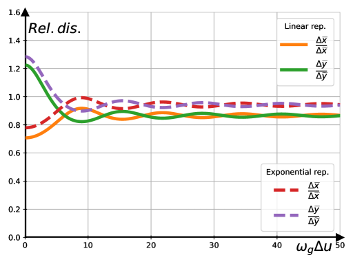
Figure 3: Relative distances $\Delta{\bar{x}}/\Delta{\tilde{x}}$ and $\Delta{\bar{y}}/\Delta{\tilde{y}}$ as function of $\Delta u$ in the diagonal basis $(\Delta\tilde{x}\;\;\Delta\tilde{y})^{T}$.

Note the explicit $i\epsilon$ prescriptions in (3.11), which give rise to the imaginary parts of the Wightman functions, and which can be traced back to the requirement that the integrals in (7.19–7.20) converge. From the Wightman functions (3.11) one can then construct the Feynman propagator in the standard way. In lightcone coordinates we have,

$$i\Delta_{F,LC}(x;x^{\prime})\!\!\! \equiv \!\!\!\Theta(\Delta u)i\Delta^{(+)}(x;x^{\prime})\!+\!\Theta(-\Delta u)i\Delta^{(-)}(x;x^{\prime})$$ (3.25)

$$= \!\!\frac{\hbar m^{D-2}}{(2\pi)^{\frac{D}{2}}[\gamma(u)\gamma(u^{\prime})]^{\frac{1}{4}}\sqrt{\Upsilon(u;u^{\prime})}}\frac{K_{\frac{D-2}{2}}\big{(}m\sqrt{\Delta{\bar{x}}_{F,LC}^{2}}\,\big{)}}{\big{(}m\sqrt{\Delta{\bar{x}}_{F,LC}^{2}}\big{)}^{\frac{D-2}{2}}},\qquad\;\;$$

and in Cartesian coordinates,

$$i\Delta_{F}(x;x^{\prime})\!\! \equiv \!\!\Theta(\Delta t)i\Delta^{(+)}(x;x^{\prime})+\Theta(-\Delta t)i\Delta^{(-)}(x;x^{\prime})$$ (3.26)

$$= \!\!\frac{\hbar m^{D-2}}{(2\pi)^{\frac{D}{2}}[\gamma(u)\gamma(u^{\prime})]^{\frac{1}{4}}\sqrt{\Upsilon(u;u^{\prime})}}\frac{K_{\frac{D-2}{2}}\big{(}m\sqrt{\Delta{\bar{x}}_{F}^{2}}\,\big{)}}{\big{(}m\sqrt{\Delta{\bar{x}}_{F}^{2}}\big{)}^{\frac{D-2}{2}}}\,.\qquad$$

Both propagators (3.25–3.26) are suitable for perturbative studies, the former for the initial value problem defined on a $u={\rm constant}$ hypersurface, the latter on a $t={\rm constant}$ hypersurface. However, the two $i\epsilon$ prescriptions differ,

$$\Delta{\bar{x}}_{F,LC}^{2}(x;x^{\prime})\!\! = \!\!-(|\Delta u|-i\epsilon)(\pm\Delta v-i\epsilon)\!+\!\|\Delta\vec{\bar{x}}_{\perp}\|^{2}$$

$$\Delta{\bar{x}}_{F}^{2}(x;x^{\prime})\!\! = \!\!-(|\Delta t|-i\epsilon)^{2}\!+\!\|\Delta\vec{\bar{x}}\|^{2}\,,$$ (3.27)

and they are illustrated in figure 4.

 

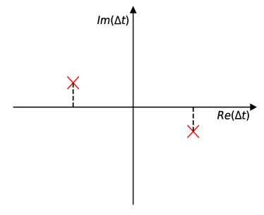
Figure 4: Left panel: The standard $i\epsilon$ prescription for the Feynman propagator. Right panel: The $i\epsilon$ prescription for the Feynman propagator in lightcone coordinates.

That means that the imaginary parts of the propagators are different. Both prescriptions are legitimate however, as they are designated to study inequivalent perturbative evolution problems.

From Eqs. (3.25–3.26) one easily obtains the corresponding Dyson propagators,

$$i\Delta_{D,LC}(x;x^{\prime})=\big{[}i\Delta_{F,LC}(x;x^{\prime})\big{]}^{*}\,,\qquad i\Delta_{D}(x;x^{\prime})=\big{[}i\Delta_{F}(x;x^{\prime})\big{]}^{*}\,,\qquad$$ (3.28)

which can be used in in-out problems to study evolution of out states backwards in time. Furthermore, the Dyson propagator is an essential ingredient for studying perturbative time evolution of Hermitian operators in weakly interacting quantum field theories.

Exponential representation. In this representation the gravitational waves are written as in (1.6), or equivalently in Eq. (1.16), such that for nonpolarized gravitational waves the Klein-Gordon equation (3.1) reduces to,

$$\hskip-8.5359pt\bigg{\{}\!-4\partial_{v}\partial_{u}\!+\!\cosh(\tilde{h})\left(\partial_{x}^{2}\!+\!\partial_{y}^{2}\right)\!-\!\frac{\sinh(\tilde{h})}{\tilde{h}}\left[\tilde{h}_{+}\cos(\omega_{g}u)(\partial_{x}^{2}\!-\!\partial_{y}^{2})\!+\!2\tilde{h}_{\times}\sin(\omega_{g}u)\partial_{x}\partial_{y}\right]$$

$$\hskip 142.26378pt\!+\,\sum_{i=3}^{D-2}\partial_{i}^{2}\!-\!m^{2}\bigg{\}}\hat{\phi}(u,\vec{x}_{\perp},v)=0,\hskip-8.5359pt$$ (3.29)

where we made use of ${\rm det}[g_{ij}]=1$. The mode equations are then,

$$\hskip-28.45274pt\Bigg{(}\partial_{u}\!\pm\!\frac{i}{2\Omega_{\mp}}\Big{[}(\cosh(\tilde{h})\!-\!1)(k_{x}^{2}\!+\!k_{y}^{2})\!-\!\sinh(\tilde{h})\Big{(}\!\cos(\omega_{g}u)(k_{x}^{2}\!-\!k_{y}^{2})\!+\!2\sin(\omega_{g}u)k_{x}k_{y}\Big{)}\Big{]}\!\pm\!\frac{i}{2}\Omega_{\pm}\Bigg{)}\phi_{\pm}(u,\vec{k})=0\,,\hskip 2.84544pt$$

(3.30)

where we made use of, $\tilde{h}_{+}=\tilde{h}_{\times}=\tilde{h}$. The mode functions can be then written in the form (3.7), with

$$\phi_{\pm}(u,\vec{k})\!\! = \!\!\sqrt{\!\frac{\hbar}{2\omega}}\exp\bigg{\{}\!\mp\frac{i}{2}\bigg{[}\Omega_{\pm}(\vec{k}\,)u+\frac{\Psi(u)}{\Omega_{\mp}(\vec{k}\,)}\bigg{]}\bigg{\}}\,,\qquad$$ (3.31)

$$\Psi(u)\!\! = \!\!(\cosh(\tilde{h})\!-\!1)(k_{x}^{2}\!+\!k_{y}^{2})u-\sinh(\tilde{h})\frac{\sin(\omega_{g}u)}{\omega_{g}}(k_{x}^{2}\!-\!k_{y}^{2})\!+\!2\sinh(\tilde{h})\frac{\cos(\omega_{g}u)}{\omega_{g}}(k_{x}k_{y})\,,\quad$$ (3.32)

From this and Eq. (7.38) we can easily evaluate elements of the deformation matrix ${\mathbf{\Upsilon}}$,

$$\Upsilon_{{}_{x}\atop{}^{y}}(u;u^{\prime})\!\! = \!\!\cosh(\tilde{h})\mp\sinh(\tilde{h})\frac{\sin(\omega_{g}u)-\sin(\omega_{g}u^{\prime})}{\omega_{g}\Delta u}\,,\qquad$$

$$\Upsilon_{xy}(u;u^{\prime})\!\! = \!\!\sinh(\tilde{h})\frac{\cos(\omega_{g}u)-\cos(\omega_{g}u^{\prime})}{\omega_{g}\Delta u}\,,$$ (3.33)

and its determinant evaluates to,

$$\Upsilon(u;u^{\prime})=\Upsilon_{x}\Upsilon_{y}-\Upsilon_{xy}^{2}=\cosh^{2}(\tilde{h})-\sinh^{2}(\tilde{h})\,j_{0}^{2}\Big{(}\frac{\omega_{g}\Delta u}{2}\Big{)}\,.\qquad$$ (3.34)

At coincidence ($\Delta u=0$) this evaluates to one, $\Upsilon(u;u)=1$, as was expected. As $|\Delta u|$ increases, $\Upsilon(u;u^{\prime})$ increases, plateauing at $\Upsilon\rightarrow\cosh^{2}(\tilde{h})$ when $|\Delta u|\rightarrow\infty$.

3.2 Polarized gravitational waves

Linear representation. General polarized gravitational waves are characterized by Eq. (1.3) (see also Eq. (1.4)), but without any relation between the amplitudes $h_{+}$, $h_{\times}$ and the corresponding phases $\psi_{+}$ and $\psi_{\times}$. The scalar field operator obeys (from Eq. (3.1)),

$$\left\{\!-4\partial_{v}\partial_{u}\!+\!\frac{(1\!-\!h_{+}c_{+}(u))\partial_{x}^{2}\!+\!(1\!+\!h_{+}c_{+}(u))\partial_{y}^{2}\!-\!2h_{\times}c_{\times}(u)\partial_{x}\partial_{y}}{1\!-\!h_{+}^{2}c_{+}^{2}(u)\!-\!h_{\times}^{2}c_{\times}^{2}(u)}\!+\!\sum_{i=3}^{D-2}\partial_{i}^{2}\!-\!m^{2}\right\}\!\big{[}\big{(}\gamma(u)\big{)}^{\frac{1}{4}}\hat{\phi}(u,\vec{x}_{\perp},v)\big{]}=0\,,\qquad$$ (3.35)

where $\gamma(u)\equiv 1-h_{+}^{2}c_{+}^{2}(u)-h_{\times}^{2}c_{\times}^{2}(u)$ is the determinant of $h_{ij}(x)$ and we have introduced a shorthand notation,

$$c_{+}(u)=\cos(\omega_{g}u+\psi_{+})\,,\qquad c_{\times}(u)=\cos(\omega_{g}u+\psi_{\times})\,.$$ (3.36)

One of the phases, for example $\psi_{+}$, can be absorbed by shifting $u$, leading to an equivalent representation,

$$c_{+}(u)=\cos(\omega_{g}u-\psi/2)\,,\qquad c_{\times}(u)=\cos(\omega_{g}u+\psi/2)\,,\qquad(\psi\equiv\psi_{\times}-\psi_{+})\,.$$ (3.37)

Decomposing the field and its canonical momentum as in (3.2–3.3) yields the equation of motion for the mode functions (cf. Eq. (3.4)),

$$\left(\!\partial_{u}\pm\frac{i}{2\Omega_{\mp}}\left[\frac{(1\!-\!h_{+}c_{+}(u))k_{x}^{2}\!+\!(1\!+\!h_{+}c_{+}(u))k_{y}^{2}\!-\!2h_{\times}c_{\times}(u)k_{x}k_{y}}{1\!-\!h_{+}^{2}c_{+}^{2}(u)\!-\!h_{\times}^{2}c_{\times}^{2}(u)}\!-\!(k_{x}^{2}\!+\!k_{y}^{2})\right]\!\pm\frac{i}{2}\Omega_{\pm}\right)\!\big{[}\gamma(u)^{\frac{1}{4}}\phi_{\pm}(u,\vec{k})\big{]}=0\,.\quad$$ (3.38)

The solution can be formally written as (cf. Eqs. (3.7–3.7)),

$$\phi_{\pm}(u,\vec{k})\!\! = \!\!\sqrt{\frac{\hbar}{2\omega}}\frac{1}{[\gamma(u)]^{1/4}}\exp\Big{[}\mp\frac{i}{2}\Big{(}\Omega_{\pm}(\vec{k}\,)u+\frac{\Psi(u)}{\Omega_{\mp}(\vec{k}\,)}\Big{)}\Big{]}\,,\qquad$$ (3.39)

$$\Psi(u)\!\! = \!\!\int^{u}{\rm d}\tilde{u}\bigg{[}\frac{[1\!-\!h_{+}\cos(\omega_{g}\tilde{u}\!-\!\psi/2)]k_{x}^{2}\!+\![1\!+\!h_{+}\cos(\omega_{g}\tilde{u}\!-\!\psi/2)]k_{y}^{2}\!-\!2h_{\times}\cos(\omega_{g}\tilde{u}\!+\!\psi/2)k_{x}k_{y}}{1\!-\!h_{+}^{2}\cos^{2}(\omega_{g}\tilde{u}\!-\!\psi/2)-h_{\times}^{2}\cos^{2}(\omega_{g}\tilde{u}\!+\!\psi/2)}$$ (3.40)

$$\!\!\hskip 42.67912pt\!-\,(k_{x}^{2}\!+\!k_{y}^{2})\bigg{]}\,,\qquad\;$$

such that, as in Eq. (3.7), $\Psi(u)\rightarrow 0$ as $h_{+}\rightarrow 0$ and $h_{\times}\rightarrow 0$.

Let us first consider the simpler case of maximally polarized gravitational waves. For the $(+)$ polarization (i.e. $h_{\times}=0$, $\psi=0$) the integral in (3.40) simplifies to a standard integral performed in Eq. (7.71) of Appendix C,

$$\Psi(u)\!\! = \!\!\int^{u}d\tilde{u}\bigg{[}\frac{k_{x}^{2}}{1+h_{+}\cos(\omega_{g}\tilde{u})}+\frac{k_{y}^{2}}{1-h_{+}\cos(\omega_{g}\tilde{u})}\bigg{]}\!-\!(k_{x}^{2}\!+\!k_{y}^{2})u$$ (3.41)

$$\!\!\hskip-45.52458pt=\frac{2}{\omega_{g}}\frac{k_{x}^{2}}{\sqrt{1\!-\!h_{+}^{2}}}\text{Arctan}\bigg{[}\sqrt{\frac{1\!-\!h_{+}}{1\!+\!h_{+}}}\!\tan\Big{(}\frac{\omega_{g}u}{2}\Big{)}\bigg{]}\!+\!\frac{2}{\omega_{g}}\frac{k_{y}^{2}}{\sqrt{1\!-\!h_{+}^{2}}}\text{Arctan}\bigg{[}\sqrt{\frac{1\!+\!h_{+}}{1\!-\!h_{+}}}\!\tan\Big{(}\frac{\omega_{g}u}{2}\Big{)}\bigg{]}\!-\!(k_{x}^{2}\!+\!k_{y}^{2})u.\qquad\;$$

This result is defined only in the interval $-\pi<\omega_{g}u<\pi$, but there is a unique analytic extension of it to the real axis, $-\infty<u<\infty$ and to the complex $u-$plane. Note first that in the limit when $h_{+}\rightarrow 0$, $\Psi(u)=0$ in the entire interval $-\pi<\omega_{g}u<\pi$, implying that its analytic extension to the complex $u-$plane is simply, $\Psi(u)=0$. When $h_{+}\neq 0$, note first that at the boundaries of the interval (when $\omega_{g}u\rightarrow\pm\pi$),

$$\Psi\Big{(}u\rightarrow\pm\frac{\pi}{\omega_{g}}\Big{)}=\pm\frac{\pi}{\omega_{g}}(k_{x}^{2}+k_{y}^{2})\left[\frac{1}{\sqrt{1-h_{+}^{2}}}-1\right]\,,\quad$$ (3.42)

such that $\Psi(u)$ increments by $\Psi(\pi/\omega_{g})-\Psi(-\pi/\omega_{g})$ accross the interval where it is defined. This can be utilized by extending the definition of ${\rm Arctan}(z)$ in Eq. (3.41) to ${\rm arctan}(z)$ defined on the whole complex plane by,

$${\rm arctan}\bigg{[}\sqrt{\frac{1\pm h_{+}}{1\mp h_{+}}}\tan\Big{(}\frac{\omega_{g}u}{2}\Big{)}\bigg{]}\equiv\begin{cases}&\!\!\!\!{\rm Arctan}\bigg{[}\sqrt{\frac{1\pm h_{+}}{1\mp h_{+}}}\tan\Big{(}\frac{\omega_{g}u-2n\pi}{2}\Big{)}\bigg{]}\!+\!\pi n,\quad\frac{(-1+2n)\pi}{\omega_{g}}<u<\frac{(1+2n)\pi}{\omega_{g}}\cr&\!\!\!\!\pi\left(n+\frac{1}{2}\right)\,,\quad{\rm when}\quad u=\frac{(1+2n)\pi}{\omega_{g}}\,,\quad(n\in\mathbb{Z})\cr\end{cases},\quad\;$$ (3.43)

where $\mathbb{Z}$ denotes the set of integers. The analytically extended solution of (3.41) can then be written as,

$$\Psi(u)\!\! = \!\!\frac{2}{\omega_{g}}\frac{k_{x}^{2}}{\sqrt{1\!-\!h_{+}^{2}}}\text{arctan}\bigg{[}\sqrt{\frac{1\!-\!h_{+}}{1\!+\!h_{+}}}\tan\Big{(}\frac{\omega_{g}u}{2}\Big{)}\bigg{]}\!+\!\frac{2}{\omega_{g}}\frac{k_{y}^{2}}{\sqrt{1\!-\!h_{+}^{2}}}\text{arctan}\bigg{[}\sqrt{\frac{1\!+\!h_{+}}{1\!-\!h_{+}}}\tan\Big{(}\frac{\omega_{g}u}{2}\Big{)}\bigg{]}\quad$$ (3.44)

$$- \!\!(k_{x}^{2}\!+\!k_{y}^{2})u.$$

and its form is illustrated in figure 5.

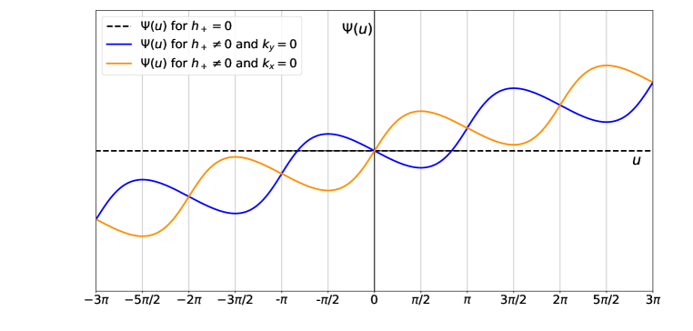
Figure 5: The analytically extended phase function $\Psi(u)$ defined in Eq. (3.44). The choice of the parameters is $k^{2}_{x}/\omega_{g}^{2}=k_{y}^{2}/\omega_{g}^{2}=1$, and $h_{+}=1/2$ is chosen (unrealistically) large in order to make its effect more visible.

The second case of interest is the $(\times)$-polarized wave (for which $h_{+}=0$). In this case, the phase modulation integral (3.40) simplifies to,

$$\Psi(u)\!\! = \!\!\int^{u}d\tilde{u}\bigg{[}\frac{k_{x}^{2}\!+\!k_{y}^{2}}{1-h_{\times}^{2}\cos^{2}(\omega_{g}\tilde{u})}\!-\!\frac{2h_{\times}\cos(\omega_{g}\tilde{u})k_{x}k_{y}}{1-h_{\times}^{2}\cos^{2}(\omega_{g}\tilde{u})}\bigg{]}\!-\!(k_{x}^{2}\!+\!k_{y}^{2})u\,,\quad$$ (3.45)

$$= \!\!\frac{k_{x}^{2}\!+\!k_{y}^{2}}{\omega_{g}\sqrt{1\!-\!h_{\times}^{2}}}\text{arctan}\bigg{[}\frac{1}{\sqrt{1\!-\!h_{\times}^{2}}}\tan(\omega_{g}u)\bigg{]}\!-\!\frac{2k_{x}k_{y}}{\omega_{g}\sqrt{1\!-\!h_{\times}^{2}}}\text{arctan}\bigg{[}\frac{h_{\times}}{\sqrt{1\!-\!h_{\times}^{2}}}\sin(\omega_{g}u)\bigg{]}\!\!-\!(k_{x}^{2}\!+\!k_{y}^{2})u,\qquad\;\;$$

where we set the (physically irrelevant) phase $\psi=0$, and made use of the integrals (7.72–7.73) in Appendix C, whereby we analytically extended ${\rm Arctan}(z)$ as in Eq. (3.43).

The integral in Eq. (3.40) for the general case can be rewritten using the substitution $t=\tan(\omega_{g}u-\frac{\psi}{2})$ to obtain,

$$\Psi(u)=-(k_{x}^{2}+k_{y}^{2})u+\frac{1}{\omega_{g}}\int\frac{\text{d}t}{\sqrt{1+t^{2}}}\frac{(k_{x}^{2}+k_{y}^{2})\sqrt{1+t^{2}}+h_{+}(k_{y}^{2}-k_{x}^{2})-2h_{\times}k_{x}k_{y}\big{[}c_{\psi}-s_{\psi}t\big{]}}{1-h_{+}^{2}-h_{\times}^{2}c_{\psi}^{2}+2h_{\times}^{2}c_{\psi}s_{\psi}t+(1-h_{\times}^{2}s_{\psi}^{2})t^{2}}\,,\quad$$ (3.46)

where $c_{\psi}$ and $s_{\psi}$ are abbreviations of $\cos(\psi)$ and $\sin(\psi)$, respectively. Using integral (7.74) given in Appendix C, $\Psi(u)$ evaluates to,

$$\Psi(u)\!\! = \!\!\frac{1}{\omega_{g}\sqrt{1-(h_{+}^{2}+h_{\times}^{2})+h_{+}^{2}h_{\times}^{2}s_{\psi}^{2}}}\Bigg{\{}\!\big{(}k_{x}^{2}+k_{y}^{2}\big{)}\text{Arctan}\Bigg{(}\frac{h_{\times}^{2}s_{\psi}c_{\psi}+(1-h_{\times}^{2}s_{\psi}^{2})\tan(\omega_{g}u-\frac{\psi}{2})}{\sqrt{1-(h_{+}^{2}+h_{\times}^{2})+h_{+}^{2}h_{\times}^{2}s_{\psi}^{2}}}\Bigg{)}$$ (3.47)

$$\hskip-39.83368pt+\,\frac{i\big{[}\!\!-\!2h_{\times}k_{x}k_{y}c_{\psi}\!+\!2ih_{\times}k_{x}k_{y}s_{\psi}\sqrt{1\!-\!(h_{+}^{2}\!+\!h_{\times}^{2})\!+\!h_{+}^{2}h_{\times}^{2}s_{\psi}^{2}}\!-\!(1\!-\!h_{\times}^{2}s_{\psi}^{2})\big{(}k_{x}^{2}\!-\!k_{y}^{2}\big{)}h_{+}\big{]}\text{Arctanh}[g(u)]}{2\sqrt{h_{+}^{2}\!+\!h_{\times}^{2}\!-\!h_{\times}^{2}s_{\psi}^{2}(2\!+\!h_{+}^{2}\!+\!h_{\times}^{2})\!-\!2ih_{\times}^{2}c_{\psi}s_{\psi}\sqrt{1\!-\!(h_{+}^{2}\!+\!h_{\times}^{2})\!+\!h_{+}^{2}h_{\times}^{2}s_{\psi}^{2}}}}\!+{\rm c.c.}\!\Bigg{\}}\;$$

$$\hskip-36.98866pt-\,\big{(}k_{x}^{2}+k_{y}^{2}\big{)}u\,,\quad$$

where ${\rm c.c.}$ denotes the complex conjugate of the term in the second line and the function $g(u)$ is defined by,

$$g(u)\equiv\frac{(1\!-\!h_{\times}s_{\psi}^{2})\cos(\omega_{g}\!-\!\psi/2)\!+\!\left[i\sqrt{1\!-\!(h_{+}^{2}\!+\!h_{\times}^{2})\!+\!h_{+}^{2}h_{\times}^{2}s_{\psi}^{2}}\!-\!h_{\times}^{2}c_{\psi}s_{\psi}\right]\sin(\omega_{g}u\!-\!\psi/2)}{\sqrt{h_{+}^{2}\!+\!h_{\times}^{2}\!-\!h_{\times}^{2}s_{\psi}^{2}(2\!+\!h_{+}^{2}\!+\!h_{\times}^{2})\!-\!2ih_{\times}^{2}c_{\psi}s_{\psi}\sqrt{1\!-\!(h_{+}^{2}\!+\!h_{\times}^{2})\!+\!h_{+}^{2}h_{\times}^{2}s_{\psi}^{2}}}}.\;$$ (3.48)

The corresponding ${\mathbf{\Upsilon}}$ matrix can be formally written from Eq. (3.40) as,

$${\Upsilon}_{{}_{x}\atop{}^{y}}(u;u^{\prime})\!\! = \!\!\frac{1}{\Delta u}\left[\int^{u}{\rm d}\tilde{u}\frac{1\!\mp\!h_{+}\cos(\omega_{g}\tilde{u}\!-\!\psi/2)}{1\!-\!h_{+}^{2}\cos^{2}(\omega_{g}\tilde{u}\!-\!\psi/2)-h_{\times}^{2}\cos^{2}(\omega_{g}\tilde{u}\!+\!\psi/2)}-(u\rightarrow u^{\prime})\right]\,,\;$$

$${\Upsilon}_{xy}(u;u^{\prime})\!\! = \!\!\frac{1}{\Delta u}\left[\int^{u}{\rm d}\tilde{u}\frac{\!-\!h_{\times}\cos(\omega_{g}\tilde{u}\!+\!\psi/2)}{1\!-\!h_{+}^{2}\cos^{2}(\omega_{g}\tilde{u}\!-\!\psi/2)-h_{\times}^{2}\cos^{2}(\omega_{g}\tilde{u}\!+\!\psi/2)}-(u\rightarrow u^{\prime})\right]\,.\qquad\;$$ (3.49)

This can be integrated and the result follows from Eq. (3.47),

$${\Upsilon}_{{}_{x}\atop{}^{y}}\!\! = \!\!\frac{1}{\omega_{g}\Delta u\sqrt{1-(h_{+}^{2}+h_{\times}^{2})+h_{+}^{2}h_{\times}^{2}s_{\psi}^{2}}}\left\{\!\text{arctan}\Bigg{(}\frac{h_{\times}^{2}s_{\psi}c_{\psi}+(1-h_{\times}^{2}s_{\psi}^{2})\tan(\omega_{g}u-\frac{\psi}{2})}{\sqrt{1-(h_{+}^{2}+h_{\times}^{2})+h_{+}^{2}h_{\times}^{2}s_{\psi}^{2}}}\Bigg{)}\right.$$

$$\hskip-5.69046pt\left.\mp\,i\frac{(1\!-\!h_{\times}^{2}s_{\psi}^{2})h_{+}\text{arctanh}[g(u)]}{2\sqrt{h_{+}^{2}\!+\!h_{\times}^{2}\!-\!h_{\times}^{2}s_{\psi}^{2}(2\!+\!h_{+}^{2}\!+\!h_{\times}^{2})\!-\!2ih_{\times}^{2}c_{\psi}s_{\psi}\sqrt{1\!-\!(h_{+}^{2}\!+\!h_{\times}^{2})\!+\!h_{+}^{2}h_{\times}^{2}s_{\psi}^{2}}}}\!+{\rm c.c.}-(u\rightarrow u^{\prime})\!\right\},\;$$

$${\Upsilon}_{xy}\!\! = \!\!\frac{1}{\omega_{g}\Delta u\sqrt{1-(h_{+}^{2}+h_{\times}^{2})+h_{+}^{2}h_{\times}^{2}s_{\psi}^{2}}}$$ (3.50)

$$\times \!\!\!\!\left\{-\frac{\big{[}ic_{\psi}\!+\!s_{\psi}\sqrt{1\!-\!(h_{+}^{2}\!+\!h_{\times}^{2})\!+\!h_{+}^{2}h_{\times}^{2}s_{\psi}^{2}}\,\big{]}h_{\times}\text{Arctanh}[g(u)]}{\sqrt{h_{+}^{2}\!+\!h_{\times}^{2}\!-\!h_{\times}^{2}s_{\psi}^{2}(2\!+\!h_{+}^{2}\!+\!h_{\times}^{2})\!-\!2ih_{\times}^{2}c_{\psi}s_{\psi}\sqrt{1\!-\!(h_{+}^{2}\!+\!h_{\times}^{2})\!+\!h_{+}^{2}h_{\times}^{2}s_{\psi}^{2}}}}\!+{\rm c.c.}-(u\rightarrow u^{\prime})\!\right\},\qquad\;$$

and the special cases of singly-polarized gravitational waves can be obtained by taking the suitable limits of this general result. Alternatively, one can extract the corresponding matrices ${\mathbf{\Upsilon}}$ from Eq. (3.44)

$${\mathbf{\Upsilon}}_{+}=\frac{2}{\omega_{g}\Delta u}\frac{1}{\sqrt{1\!-\!h_{+}^{2}}}\left\{\left(\!\!\begin{array}[]{cc}\text{arctan}\bigg{[}\sqrt{\frac{1\!-\!h_{+}}{1\!+\!h_{+}}}\tan\Big{(}\frac{\omega_{g}u}{2}\Big{)}\bigg{]}&0\cr 0&\text{arctan}\bigg{[}\sqrt{\frac{1\!+\!h_{+}}{1\!-\!h_{+}}}\tan\Big{(}\frac{\omega_{g}u}{2}\Big{)}\bigg{]}\cr\end{array}\!\!\right)\!-\!(u\rightarrow u^{\prime})\right\},\;$$ (3.51)

and Eq. (3.45),

$${\mathbf{\Upsilon}}_{\times}=\frac{1}{\omega_{g}\Delta u}\frac{1}{\sqrt{1\!-\!h_{\times}^{2}}}\left\{\left(\!\!\begin{array}[]{cc}\text{arctan}\bigg{[}\frac{1}{\sqrt{1\!-\!h_{\times}^{2}}}\tan(\omega_{g}u)\bigg{]}&-\text{arctan}\bigg{[}\frac{h_{\times}}{\sqrt{1\!-\!h_{\times}^{2}}}\sin(\omega_{g}u)\bigg{]}\cr-\text{arctan}\bigg{[}\frac{h_{\times}}{\sqrt{1\!-\!h_{\times}^{2}}}\sin(\omega_{g}u)\bigg{]}&\text{arctan}\bigg{[}\frac{1}{\sqrt{1\!-\!h_{\times}^{2}}}\tan(\omega_{g}u)\bigg{]}\cr\end{array}\!\!\right)-(u\rightarrow u^{\prime})\right\},\;$$ (3.52)

respectively.

Exponential representation. Since in this purely tensorial representation (1.6), (1.16), ${\rm det}[g_{ij}]=1$ is generally true, the field operator $\hat{\phi}$ obeys Eq. (3.29), but with $\tilde{h}=\tilde{h}(u)$ a function of $u$ given in Eq. (1.12), and the waves oscillate with general phases $\psi_{\pm}$ as in Eq. (3.37).

The mode function equations (3.30) generalizes to,

$$\hskip-28.45274pt\Bigg{(}\!\partial_{u}\!\pm\!\frac{i}{2\Omega_{\mp}}\bigg{[}\big{(}\!\cosh(\tilde{h}(u))\!-\!1\big{)}(k_{x}^{2}\!+\!k_{y}^{2})$$ (3.53)

$$\hskip 34.14322pt\!-\,\frac{\sinh(\tilde{h}(u))}{\tilde{h}(u)}\Big{(}\!\tilde{h}_{+}c_{+}(u)(k_{x}^{2}\!-\!k_{y}^{2})\!+\!2\tilde{h}_{\times}c_{\times}(u)k_{x}k_{y}\Big{)}\bigg{]}\!\!\pm\!\frac{i}{2}\Omega_{\pm}\Bigg{)}\phi_{\pm}(u,\vec{k})\!=\!0\,,\hskip 28.45274pt$$

which implies the following formal solution for $\Psi(u)$,

$$\Psi(u)\!\! = \!\!\int^{u}{\rm d}\bar{u}\bigg{[}\big{(}\!\cosh(\tilde{h}(\bar{u}))\!-\!1\big{)}(k_{x}^{2}\!+\!k_{y}^{2})\!-\!\frac{\sinh(\tilde{h}(\bar{u}))}{\tilde{h}(\bar{u})}\Big{(}\!\tilde{h}_{+}c_{+}(\bar{u})(k_{x}^{2}\!-\!k_{y}^{2})\!+\!2\tilde{h}_{\times}c_{\times}(\bar{u})k_{x}k_{y}\Big{)}\bigg{]}\,,\hskip 14.22636pt$$ (3.54)

from which one can extract elements of the deformation matrix (cf. Eqs. (3.32–3.33)),

$$\Upsilon_{{}_{x}\atop{}^{y}}(u;u^{\prime})\!\! = \!\!\frac{1}{\Delta u}\bigg{\{}\left[\int^{u}{\rm d}\bar{u}\cosh(\tilde{h}(\bar{u}))-\int^{u^{\prime}}{\rm d}\bar{u}\cosh(\tilde{h}(\bar{u}))\right]$$

$$\mp \!\!\tilde{h}_{+}\left[\int^{u}{\rm d}\bar{u}\frac{\sinh(\tilde{h}(\bar{u}))}{\tilde{h}(\bar{u})}\cos\Big{(}\omega_{g}\bar{u}\!-\!\frac{\psi}{2}\Big{)}-\int^{u^{\prime}}{\rm d}\bar{u}\frac{\sinh(\tilde{h}(\bar{u}))}{\tilde{h}(\bar{u})}\cos\Big{(}\omega_{g}\bar{u}\!-\!\frac{\psi}{2}\Big{)}\right]\bigg{\}}\,,\qquad$$

$$\Upsilon_{xy}(u;u^{\prime})\!\! = \!\!-\frac{\tilde{h}_{\times}}{\Delta u}\left[\int^{u}{\rm d}\bar{u}\frac{\sinh(\tilde{h}(\bar{u}))}{\tilde{h}(\bar{u})}\cos\Big{(}\omega_{g}\bar{u}\!+\!\frac{\psi}{2}\Big{)}-\int^{u^{\prime}}{\rm d}\bar{u}\frac{\sinh(\tilde{h}(\bar{u}))}{\tilde{h}(\bar{u})}\cos\Big{(}\omega_{g}\bar{u}\!+\!\frac{\psi}{2}\Big{)}\right]\,,\qquad\;$$ (3.55)

in terms of which the determinant can be written as in Eq. (3.34), $\Upsilon(u;u^{\prime})=\Upsilon_{x}\Upsilon_{y}-\Upsilon_{xy}^{2}$. The integrals (3.55) cannot be evaluated for general gravitational waves (see footnote 19). However, one can expand the $\cosh(\tilde{h}(u))$ and $\sinh(\tilde{h}(u))$ in (3.55) in powers of $\tilde{h}(u)$ and perform the integrals order by order. Keeping the terms up to the second order in the gravitational wave amplitude, one obtains,

$$\Upsilon_{{}_{x}\atop{}^{y}}(u;u^{\prime})\!\! = \!\!\left(\!1+\frac{\tilde{h}_{+}^{2}+\tilde{h}_{\times}^{2}}{2}\right)+\frac{\tilde{h}_{+}^{2}[\sin(2\omega_{g}u\!-\!\psi)\!-\!\sin(2\omega_{g}u^{\prime}\!-\!\psi)]\!+\!\tilde{h}_{\times}^{2}[\sin(2\omega_{g}u\!+\!\psi)\!-\!\sin(2\omega_{g}u^{\prime}\!+\!\psi)]}{4\omega_{g}\Delta u}\,,\;\;$$

$$\pm \!\!\,\frac{\tilde{h}_{+}}{\omega_{g}\Delta u}\left[\sin\Big{(}\omega_{g}u\!-\!\frac{\psi}{2}\Big{)}-\sin\Big{(}\omega_{g}u^{\prime}\!-\!\frac{\psi}{2}\Big{)}\right]+{\cal O}(\tilde{h}_{+}^{3},\tilde{h}_{+}\tilde{h}_{\times}^{2})$$

$$\Upsilon_{xy}(u;u^{\prime})\!\! = \!\!\frac{\tilde{h}_{\times}}{\omega_{g}\Delta u}\left[\sin\Big{(}\omega_{g}u\!+\!\frac{\psi}{2}\Big{)}-\sin\Big{(}\omega_{g}u^{\prime}\!+\!\frac{\psi}{2}\Big{)}\right]+{\cal O}(\tilde{h}_{\times}^{3},\tilde{h}_{\times}\tilde{h}_{+}^{2})\,,\qquad$$ (3.56)

where we made use of, $\tilde{h}(u)^{2}=\tilde{h}_{+}^{2}\cos^{2}(\omega_{g}u-\psi/2)+\tilde{h}_{\times}^{2}\cos^{2}(\omega_{g}u+\psi/2)$. From Eq. (3.56) one sees that the general structure of ${\mathbf{\Upsilon}}$ is,

$${\mathbf{\Upsilon}}(u;u^{\prime})={\mathbf{A}}_{0}+\sum_{n=1}^{\infty}\left[{\mathbf{A}}_{n}\frac{\cos(n\omega_{g}u)-\cos(n\omega_{g}u^{\prime})}{\omega_{g}\Delta u}+{\mathbf{B}}_{n}\frac{\sin(n\omega_{g}u)-\sin(n\omega_{g}u^{\prime})}{\omega_{g}\Delta u}\right]\,,\qquad\;$$ (3.57)

where the matrix-valued coefficients are (up to the quadratic order in $\tilde{h}_{+}$ and $\tilde{h}_{\times}$),

$${\mathbf{A}}_{0}\!\! = \!\!\left(\!\!\begin{array}[]{cc}1&0\cr 0&1\cr\end{array}\!\!\right)\left(\!1+\frac{\tilde{h}_{+}^{2}\!+\!\tilde{h}_{\times}^{2}}{2}\right)\,,\qquad{\mathbf{A}}_{1}=\left(\!\!\begin{array}[]{cc}-\tilde{h}_{+}&\tilde{h}_{\times}\cr\tilde{h}_{\times}&\tilde{h}_{+}\cr\end{array}\!\!\right)\sin(\psi/2)\,,\qquad{\mathbf{A}}_{2}=\left(\!\!\begin{array}[]{cc}1&0\cr 0&1\cr\end{array}\!\!\right)\frac{-\tilde{h}_{+}^{2}\!+\!\tilde{h}_{\times}}{4}\sin(\psi)\quad$$ (3.64)

$${\mathbf{B}}_{1}\!\! = \!\!\left(\!\!\begin{array}[]{cc}\tilde{h}_{+}&\tilde{h}_{\times}\cr\tilde{h}_{\times}&-\tilde{h}_{+}\cr\end{array}\!\!\right)\cos(\psi/2)\,,\qquad{\mathbf{B}}_{2}=\left(\!\!\begin{array}[]{cc}1&0\cr 0&1\cr\end{array}\!\!\right)\frac{\tilde{h}_{+}^{2}+\tilde{h}_{\times}^{2}}{4}\cos(\psi)\,,\qquad$$ (3.69)

which are all time independent. The coincident limit of (3.57) is simply,

$${\mathbf{\Upsilon}}(u;u)={\mathbf{A}}_{0}+\sum_{n=1}^{\infty}\big{[}n\big{(}\!-\!{\mathbf{A}}_{n}\sin(n\omega_{g}u)+{\mathbf{B}}_{n}\cos(n\omega_{g}u)\big{)}\big{]}\,,\qquad\;$$ (3.70)

from which one can also calculate the determinant in the usual way, $\Upsilon(u;u)=\Upsilon_{x}(u;u)\Upsilon_{y}(u;u)-\Upsilon_{xy}(u;u)^{2}=1$ (cf. Eq. (7.87)).

The Wightman functions and the propagator for polarized gravitational waves are then obtained by inserting the deformation matrix ${\mathbf{\Upsilon}}$ from this subsection into Eqs. (3.11) and (3.25–3.26), respectively.

In this section we considered planar gravitational waves generated by a single binary system (or several binary systems) orbiting in the $xy-$plane. While this situation is general in $D=4$, in $D$ dimensions more baroque situations are possible. Gravitational waves can be generated by multiple binary systems, and their gravitational waves can be decomposed into $(D-2)(D-3)/2$ orthogonal planes. Such systems can be analyzed, and general expressions can be obtained for the phase functions $\Psi(u)$ by expanding in powers of the gravitational wave amplitudes akin to Eq. (3.57). Details of such an analysis are given in Appendix D.

4 One-loop effective action and scalar mass

In this section we perform two simple one-loop calculations: the one-loop effective action and the one-loop scalar mass. As we will now show, planar gravitational waves do not contribute to these two objects.

4.1 One-loop effective action

It is of interest to investigate whether gravitational waves can have an effect on the one-loop effective action, whose Feynman diagram is shown in the left panel of figure 6. The one-loop effective action for a real scalar field is of the form,

$$\Gamma_{1}=\frac{i}{2}{\rm Tr}\log\Bigg{[}\frac{\sqrt{-g}\big{(}\Box-m^{2}\big{)}}{\mu^{2}}\Bigg{]}=-\frac{1}{2}\int{\rm d}^{D}x\sqrt{-g}\int^{m^{2}}{\rm d}\bar{m}^{2}\left[i\Delta_{F}(x;x)\right]\,,$$ (4.1)

where $i\Delta_{F}(x;x^{\prime})$ denotes the scalar propagator at spacetime coincidence, and $\mu$ is an arbitrary energy scale. The second equality in (4.1) follows from taking a derivative with respect to $m^{2}$ and integrating, and the two actions are identical up to an irrelevant field independent integration constant.

         

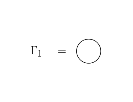
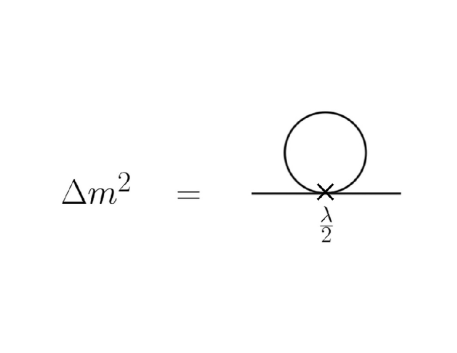
Figure 6: Left panel: The Feynman diagram for the one-loop effective action. Right panel: The Feynman diagram for the one-loop scalar self-mass.

Note firstly that the coincident Wightman functions (3.11) are both real, implying that they are equal to the coincident Feynman propagators (3.25) and (3.26),

$$i\Delta_{F}(x;x)=i\Delta^{(\pm)}(x;x)=\frac{\hbar m^{D-2}}{(2\pi)^{\frac{D}{2}}\sqrt{\gamma(u)\Upsilon(u;u)}}\left[\frac{K_{\frac{D-2}{2}}\big{(}m\sqrt{\Delta{\bar{x}}_{(\pm)}^{2}}\,\big{)}}{\big{(}m\sqrt{\Delta{\bar{x}}_{(\pm)}^{2}}\,\big{)}^{\frac{D-2}{2}}}\right]_{x^{\prime}\rightarrow x}\,,$$ (4.2)

The scalar propagator at spacetime coincidence can be obtained from the following power-series representation of Bessel function of the second kind,

$$\frac{K_{\nu}(z)}{z^{\nu}}=\frac{\Gamma(\nu)\Gamma(1-\nu)}{2^{1+\nu}}\left[\sum_{n=0}^{\infty}\frac{(z/2)^{2n-2\nu}}{n!\Gamma(n+1-\nu)}-\sum_{n=0}^{\infty}\frac{(z/2)^{2n}}{n!\Gamma(n+1+\nu)}\right]$$ (4.3)

where $z=m\sqrt{\Delta x_{\pm}^{2}}$ and $\nu=(D-2)/2$. Recalling that in dimensional regularization $D-$dependent powers of $z$ do not contribute at coincidence, one arrives at,

$$i\Delta_{F}(x;x)=\frac{m^{D-2}}{(4\pi)^{D/2}\sqrt{\gamma(u)\Upsilon(u;u)}}\Gamma\Big{(}1-\frac{D}{2}\Big{)}\,,\qquad\Gamma\Big{(}1-\frac{D}{2}\Big{)}=\frac{2}{D\!-\!4}+\gamma_{E}-1+{\cal O}(D-4)\,.$$ (4.4)

The next step is to calculate the product $\gamma(u)\Upsilon(u;u)$. In linear representation for nonpolarized gravitational waves, one has $\gamma(u)=(1-h^{2})$ and from Eq. (7.69) one finds, $\Upsilon(u;u)=1/(1-h^{2})$, such that,

$$\gamma(u)\Upsilon(u;u)=1\,.$$ (4.5)

In fact, this result holds for more general polarized gravitational waves. To show that, one can apply the l’Hospital rule to Eq. (3.49) to obtain,

$${\Upsilon}_{{}_{x}\atop{}^{y}}(u;u)\!\! = \!\!\frac{1\!\mp\!h_{+}\cos(\omega_{g}u\!-\!\psi/2)}{1\!-\!h_{+}^{2}\cos^{2}(\omega_{g}u\!-\!\psi/2)-h_{\times}^{2}\cos^{2}(\omega_{g}u\!+\!\psi/2)}\,,\;$$

$${\Upsilon}_{xy}(u;u)\!\! = \!\!\frac{\!-\!h_{\times}\cos(\omega_{g}u\!+\!\psi/2)}{1\!-\!h_{+}^{2}\cos^{2}(\omega_{g}u\!-\!\psi/2)-h_{\times}^{2}\cos^{2}(\omega_{g}u\!+\!\psi/2)}\,,\qquad\;$$ (4.6)

from which one easily obtains,

$${\Upsilon}(u;u)=\frac{1}{1\!-\!h_{+}^{2}\cos^{2}(\omega_{g}u\!-\!\psi/2)-h_{\times}^{2}\cos^{2}(\omega_{g}u\!+\!\psi/2)}\equiv\frac{1}{1-h(u)^{2}}\,,\qquad$$ (4.7)

On the other hand, $\gamma(u)={\rm det}[g_{ij}]=1-h(u)^{2}$, such that,

$$\gamma(u){\Upsilon}(u;u)=1\,.\qquad$$ (4.8)

The calculation in exponential representation is even easier, as $\gamma(u)=1$ and $\Upsilon(u;u)=1$, which can be obtained by applying the l’Hospital rule to Eq. (3.55). In fact, in Appendix D we show that $\Upsilon(u;u)=1$ holds true for even more general gravitational waves in exponential representation. The significant implication of this simple calculation is that planar gravitational waves do not influence scalar field coincident propagator (4.4), i.e. we have,

$$i\Delta_{F}(x;x)=\frac{\hbar m^{D-2}}{(4\pi)^{D/2}}\Gamma\Big{(}1-\frac{D}{2}\Big{)}\,,\qquad\Gamma\Big{(}1-\frac{D}{2}\Big{)}=\frac{2}{D\!-\!4}+\gamma_{E}-1+{\cal O}(D-4)\,.\qquad$$ (4.9)

Inserting this into (4.1) gives,

$$\Gamma_{1}\!\! = \!\!\int{\rm d}^{D}x\sqrt{-g}\frac{\hbar m^{D}}{2(4\pi)^{D/2}}\Gamma\Big{(}\!-\frac{D}{2}\Big{)}$$ (4.10)

$$= \!\!-\int{\rm d}^{D}x\!\sqrt{-g}\frac{\hbar m^{4}}{64\pi^{2}}\left[\frac{2\mu^{D-4}}{D\!-\!4}+\ln\Big{(}\frac{m^{2}}{4\pi\mu^{2}}\Big{)}+\gamma_{E}-\frac{3}{2}\right]\,.$$

From this we see that the counterterm action is of the cosmological constant-type,

$$S^{\rm ct}_{1}=\int{\rm d}^{D}x\sqrt{-g}\Big{(}-\frac{\Lambda_{0}}{16\pi G_{0}}\Big{)}\,,\qquad\frac{\Lambda_{0}}{16\pi G_{0}}=-\frac{\hbar m^{4}}{32\pi^{2}}\frac{\mu^{D-4}}{D\!-\!4}\,,$$ (4.11)

where the counterterm is chosen in accordance with the minimal subtraction scheme. When (4.11) is added to (4.10) one obtains,

$$\Gamma_{1}^{\rm ren}=\int{\rm d}^{D}x\sqrt{-g}\left\{\!-\frac{\hbar m^{4}}{64\pi^{2}}\left[\ln\Big{(}\frac{m^{2}}{4\pi\mu^{2}}\Big{)}+\gamma_{E}-\frac{3}{2}\right]\right\}\,,$$ (4.12)

which is the standard vacuum result, interpreted as a positive contribution to the cosmological constant.

4.2 One-loop scalar mass

The scalar self-interaction in Eq. (1.1) contributes at the one-loop order to the scalar mass term as,

$$\Delta m^{2}\!\! = \!\!\frac{\lambda}{2}i\Delta_{F}(x;x)=\frac{\lambda\hbar m^{D-2}}{2(4\pi)^{D/2}}\Gamma\Big{(}1-\frac{D}{2}\Big{)}$$ (4.13)

$$= \!\!\frac{\lambda\hbar m^{2}}{32\pi^{2}}\left[\frac{2\mu^{D-4}}{D-4}+\ln\Big{(}\frac{m^{2}}{4\pi\mu^{2}}\Big{)}+\gamma_{E}-1\right]\,,$$

where we made use of Eq. (4.9). The corresponding Feynman diagram is shown at the right panel of figure 6. The divergence in (4.13) can be removed by the counterterm action,

$$S^{\rm ct}_{2}=\int{\rm d}^{D}x\sqrt{-g}\left[-\frac{m_{0}^{2}}{2}\phi^{2}\right]\,,\qquad m_{0}^{2}=-\frac{\lambda\hbar m^{2}}{16\pi^{2}}\frac{\mu^{D-4}}{D-4}\,,$$ (4.14)

resulting in the renormalized mass-squared contribution,

$$m^{2}_{\rm ren}=m^{2}+m_{0}^{2}+\Delta m^{2}=m^{2}+\frac{\lambda\hbar m^{2}}{32\pi^{2}}\left[\ln\Big{(}\frac{m^{2}}{4\pi\mu^{2}}\Big{)}+\gamma_{E}-1\right]\,.$$ (4.15)

From this we conclude that planar gravitational waves do not affect in any observable way the one-loop mass. This also means that the Brout-Englert-Higgs (BEH) mechanism and the Coleman-Weinberg mechanism [14] for mass generation are unaffected (at the one-loop level) by passage of gravitational waves.  The result (4.15) is in disagreement with Ref. [3], where a nonvanishing effect on the scalar field condensate was found.

5 One-loop energy-momentum tensor

The one-loop energy-momentum tensor, $T_{\mu\nu}(x)={\color[rgb]{0,0,1}(}-2/\sqrt{-g})\delta S/\delta g^{\mu\nu}(x)$, of the scalar field whose action is given in (1.1) can be written as,

$$\langle\Omega|T^{*}[\hat{T}_{\mu\nu}(x)]|\Omega\rangle\!\! = \!\!\big{\langle}\Omega\big{|}T^{*}\Big{[}(\partial_{\mu}\phi)(\partial_{\nu}\phi)+g_{\mu\nu}\Big{(}\!-\frac{1}{2}g^{\alpha\beta}(\partial_{\alpha}\phi)(\partial_{\beta}\phi)-\frac{m^{2}}{2}\phi^{2}\Big{)}\Big{]}\big{|}\Omega\big{\rangle}$$ (5.1)

$$= \!\!\Big{(}\delta_{(\mu}^{\alpha}\delta_{\nu)}^{\beta}-\frac{1}{2}g_{\mu\nu}g^{\alpha\beta}\Big{)}\Big{[}\partial_{\alpha}\partial_{\beta}^{\prime}\big{\langle}\Omega\big{|}T\left[\phi(x)\phi(x^{\prime})\right]\big{|}\Omega\big{\rangle}\Big{]}_{x^{\prime}\rightarrow x}-\frac{m^{2}}{2}\big{\langle}\Omega\big{|}T\big{[}\phi(x)^{2}\big{]}\big{|}\Omega\big{\rangle}$$

$$= \!\!\Big{(}\delta_{(\mu}^{\alpha}\delta_{\nu)}^{\beta}-\frac{1}{2}g_{\mu\nu}g^{\alpha\beta}\Big{)}\big{[}\partial_{\alpha}\partial_{\beta}^{\prime}i\Delta_{F}(x;x^{\prime})\big{]}_{x^{\prime}\rightarrow x}-\frac{m^{2}}{2}g_{\mu\nu}i\Delta_{F}(x;x)\,,\qquad\qquad\qquad$$

where $A_{(\mu}B_{\nu)}=(1/2)(A_{\mu}B_{\nu}+A_{\nu}B_{\mu})$ and we have dropped the self-interaction term which, in the absence of a scalar condensate, contributes at the two- and higher-loops only. The symbol $T^{*}$ denotes the frequently-used $T$-star product which – after the vertex derivatives have been commuted outside Heaviside functions – imposes the usual time ordering. The corresponding Feynman diagram is shown in figure 7, which is just the one-loop contribution to the graviton one-point function.

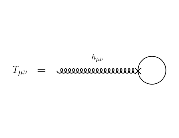
Figure 7: The Feynman diagram for the one-loop energy-momentum tensor.

Minkowski space contribution. Let us now evaluate the term $\big{[}\partial_{\alpha}\partial_{\beta}^{\prime}i\Delta_{F}(x;x^{\prime})\big{]}_{x^{\prime}\rightarrow x}$ in Eq. (5.1). To develop the intuition on what to expect, we shall first consider the Minkowski space case in lightcone coordinates, in which the metric tensor equals,

$$g_{\mu\nu}=-\frac{1}{2}\delta_{(\mu}^{\;u}\delta_{\nu)}^{\;v}(\delta_{uv}+\delta_{vu})+\delta_{(\mu}^{\;i}\delta_{\nu)}^{\;j}\delta_{ij}^{\perp}\,,$$ (5.2)

where $i,j=1,2,\cdots,D-2$. By making use of Eq. (4.3) we see that the propagator can be written as two sums, the first having $D$ dependent powers, the second integer powers. Upon taking two derivatives and then the coincident limit, only the $n=1$ term from the second (integer) series survives, yielding,

$$\big{[}\partial_{\alpha}\partial_{\beta}^{\prime}i\Delta_{F}(x;x^{\prime})\big{]}_{x^{\prime}\rightarrow x}^{\rm Mink}=-\frac{\hbar m^{D}}{D(4\pi)^{D/2}}\Gamma\left(1-\frac{D}{2}\right)g_{\alpha\beta}=-\frac{m^{2}}{D}g_{\alpha\beta}\times i\Delta_{F}(x;x)\,,\qquad$$ (5.3)

where $g_{\mu\nu}$ is given in Eq. (5.2) and the coincident propagator in (4.9) (which follows from Eqs. (4.4) and (4.8)). Acting the tensor structure in Eq. (5.1) yields a factor $-(D-2)/2$,

$$\Big{(}\delta_{(\mu}^{\alpha}\delta_{\nu)}^{\beta}-\frac{1}{2}g_{\mu\nu}g^{\alpha\beta}\Big{)}\big{[}\partial_{\alpha}\partial_{\beta}^{\prime}i\Delta_{F}(x;x^{\prime})\big{]}_{x^{\prime}\rightarrow x}^{\rm Mink}=\frac{D-2}{2D}m^{2}g_{\mu\nu}\times i\Delta_{F}(x;x)\,,\qquad\qquad$$ (5.4)

Adding to this the mass term in Eq. (5.1) one obtains,

$$\big{[}\langle\Omega|T^{*}[\hat{T}_{\mu\nu}(x)]|\Omega\rangle\big{]}^{\rm Mink}\!\! = \!\!-\frac{1}{D}m^{2}g_{\mu\nu}\times i\Delta_{F}(x;x)=-\left(\frac{1}{D}\right)\frac{\hbar m^{D}}{(4\pi)^{D/2}}\Gamma\Big{(}1-\frac{D}{2}\Big{)}g_{\mu\nu}$$ (5.5)

$$= \!\!-\frac{\hbar m^{4}}{64\pi^{2}}\left[\frac{2\mu^{D-4}}{D-4}+\ln\left(\frac{m^{2}}{4\pi\mu^{2}}\right)+\gamma_{E}-\frac{3}{2}\right]g_{\mu\nu}\,,\qquad\qquad\qquad$$

where to get the last equality we used (4.4) (with $\gamma(u)=1$ and $\Upsilon(u;u)=1$). The divergence in (5.5) can be renormalized by the cosmological constant counterterm action (4.11), which contributes to the energy-momentum tensor as,

$$T_{\mu\nu}^{(1)}=-\frac{\Lambda_{0}}{16\pi G_{0}}g_{\mu\nu}\,,\qquad$$ (5.6)

from where we infer,

$$\frac{\Lambda_{0}}{16\pi G_{0}}=-\frac{\hbar m^{4}}{32\pi^{2}}\frac{\mu^{D-4}}{D-4}\,,\qquad$$ (5.7)

which agrees with (4.11), meaning that the counterterm action (4.11) that renormalizes the one-loop effective action also renormalizes this part of the one-loop energy momentum tensor, making the renormalization procedure internally consistent. Adding (5.6) to (5.5) yields the renormalized one-loop energy-momentum tensor in Minkowski space [15],

$$\big{[}\langle\Omega|T^{*}[\hat{T}_{\mu\nu}(x)]|\Omega\rangle\big{]}^{\rm Mink,ren}\!\! = \!\!-\frac{\hbar m^{4}}{64\pi^{2}}\left[\ln\left(\frac{m^{2}}{4\pi\mu^{2}}\right)+\gamma_{E}-\frac{3}{2}\right]g_{\mu\nu}\,,\qquad\qquad\qquad$$ (5.8)

One can obtain this result also by varying Eq. (4.12) with respect to $g^{\mu\nu}$, indicating a consistency of the framework.

Nonpolarized gravitational waves.

Linear representation. Let us now study the gravitational wave contribution. We shall first consider nonpolarized gravitational waves. From the structure of the Wightman functions (3.11) and (3.14) one sees that there are two types of contributions that occur when two derivatives hit the Wightman functions: two derivatives $(\partial_{i}\partial_{j}^{\prime}$) hit the Lorentz violating distance function (3.14), and two derivatives ($\partial_{u}\partial_{u^{\prime}}$) hit the prefactor $\sqrt{\gamma(u)\gamma(u^{\prime})}\Upsilon(u;u^{\prime})$ in (3.11); .

Let us first consider the spatial contributions. Notice that acting $\partial_{i}\partial_{j}^{\prime}$ on the propagator produces (cf. Eq. (5.3)),

$$\big{[}\partial_{i}\partial_{j}^{\prime}i\Delta_{F}(x;x^{\prime})\big{]}_{x^{\prime}\rightarrow x}\!\! = \!\!-\frac{m^{2}}{D}i\Delta_{F}(x;x)({\mathbf{\Upsilon}}^{-1})_{ij}(u;u)$$ (5.9)

$$= \!\!-\frac{\hbar m^{4}}{64\pi^{2}}\left[\frac{2\mu^{D-4}}{D-4}+\ln\Big{(}\frac{m^{2}}{4\pi\mu^{2}}\Big{)}+\gamma_{E}-\frac{3}{2}\right]g_{ij}(u)\,,\qquad$$

where in the last step we made use of Eqs. (4.9), (3.23–3.24) from which it follows that,

$$({\mathbf{\Upsilon}}^{-1})_{ij}(u;u)=\delta_{ij}+h_{ij}(u)\equiv g_{ij}(u)\,,\qquad h_{ij}(u)=\left(\begin{array}[]{ccc}h\cos(\omega_{g}u)&h\sin(\omega_{g}u)&0\cdots\cr h\sin(\omega_{g}u)&-h\cos(\omega_{g}u)&0\cdots\cr 0&0&0\cdots\cr\vdots&\vdots&\!\!\!\!\!\!\vdots\cr\end{array}\right)\,.\qquad$$ (5.10)

Upon combining (5.9) with the $uv$ and $vu$ contributions (which are identical as in Minkowski space (5.5)), and inserting into Eq. (5.1) one obtains,

$$\big{[}\langle\Omega|T^{*}[\hat{T}_{\mu\nu}(x)]|\Omega\rangle\big{]}^{(1)}\!\! = \!\!-\frac{1}{D}m^{2}\times i\Delta_{F}(x;x)g_{\mu\nu}(u)$$ (5.11)

$$= \!\!-\frac{\hbar m^{4}}{64\pi^{2}}\left[\frac{2\mu^{D-4}}{D-4}+\ln\left(\frac{m^{2}}{4\pi\mu^{2}}\right)+\gamma_{E}-\frac{3}{2}\right]g_{\mu\nu}(u)\,,\qquad\qquad\qquad$$

which is covariant, but not the same as the Minkowski result in Eq. (5.5), since $g_{\mu\nu}(u)=\eta_{\mu\nu}+h_{\mu\nu}(u)$ depends on the gravitational wave strain, $h_{ij}(u)$. As in the Minkowski vacuum case, Eq. (5.11) can be renormalized by the cosmological constant counterterm action (4.11). Indeed, adding the corresponding energy momentum tensor (5.6) with the coupling constant (5.7) regularizes the energy momentum tensor in Eq. (5.11), and one obtains,

$$\big{[}\langle\Omega|T^{*}[\hat{T}_{\mu\nu}(x)]|\Omega\rangle\big{]}^{(1),\rm ren}\!\! = \!\!-\frac{\hbar m^{4}}{64\pi^{2}}\left[\ln\left(\frac{m^{2}}{4\pi\mu^{2}}\right)+\gamma_{E}-\frac{3}{2}\right]g_{\mu\nu}(u)\,,\qquad\qquad\qquad$$ (5.12)

which is identical in form to Eq. (5.8).

Let us now evaluate the second contribution, which arises from acting the $\partial_{u}\partial_{u}^{\prime}$ derivatives. To facilitate the calculation, it is useful to expand $\sqrt{\gamma(u)\gamma(u^{\prime})}\Upsilon(u;u^{\prime})$ in powers of $\Delta u$. From $\gamma(u)=1-h^{2}$ and Eq. (3.24) we find,

$$\sqrt{\gamma(u)\gamma(u^{\prime})}\Upsilon(u;u^{\prime})=\frac{1}{1-h^{2}}\bigg{\{}1\!-\!h^{2}\bigg{[}1-\frac{1}{3}\Big{(}\frac{\omega_{g}\Delta u}{2}\Big{)}^{2}\bigg{]}\bigg{\}}+{\cal O}(\Delta u^{4})\,,\quad$$ (5.13)

such that

$$\left[\partial_{u}\partial_{u}^{\prime}\Big{(}\sqrt{\gamma(u)\gamma(u^{\prime})}\Upsilon(u;u^{\prime})\Big{)}^{-\frac{1}{2}}\right]_{u^{\prime}\rightarrow u}=\frac{1}{12}\frac{\omega_{g}^{2}h^{2}}{1-h^{2}}\,,\qquad$$ (5.14)

which is the only contribution to the energy momentum tensor (5.1) from the $\partial_{u}\partial_{u^{\prime}}$ derivatives. Eq. (5.14) implies,

$$\big{[}\partial_{u}\partial_{u^{\prime}}i\Delta_{F}(x;x^{\prime})\big{]}_{x^{\prime}\rightarrow x}\!\! = \!\!\big{[}\partial_{u}\partial_{u^{\prime}}i\Delta^{(\pm)}(x;x^{\prime})\big{]}_{x^{\prime}\rightarrow x}=\frac{1}{12}\frac{\omega_{g}^{2}h^{2}}{1-h^{2}}i\Delta_{F}(x;x)$$ (5.15)

$$= \!\!\frac{\hbar m^{2}}{192\pi^{2}}\frac{\omega_{g}^{2}h^{2}}{1-h^{2}}\left[\frac{2\mu^{D-4}}{D-4}+\ln\Big{(}\frac{m^{2}}{4\pi\mu^{2}}\Big{)}+\gamma_{E}-1\right]\,,\qquad$$

where the first equality follows from the realization that when $\partial_{u}\partial_{u^{\prime}}$ act on $\Theta(\pm\Delta u)$ in the definition of the Feynman propagator, they do not produce any contribution.  Upon processing (5.15) through Eq. (5.1) one gets,

$$\big{[}\langle\Omega|T^{*}[\hat{T}_{uu}(x)]|\Omega\rangle\big{]}^{(2)}\!\! = \!\!\frac{\hbar m^{2}}{192\pi^{2}}\frac{\omega_{g}^{2}h^{2}}{1-h^{2}}\left[\frac{2\mu^{D-4}}{D-4}+\ln\Big{(}\frac{m^{2}}{4\pi\mu^{2}}\Big{)}+\gamma_{E}-1\right]\,,\qquad$$ (5.16)

which can be also written as (in Cartesian coordinates),

$$\big{[}\langle\Omega|T^{*}[\hat{T}_{\mu\nu}(x)]|\Omega\rangle\big{]}^{(2)}\!\! = \!\!\frac{m^{2}}{192\pi^{2}}\frac{\omega_{g}^{2}h^{2}}{1-h^{2}}\left[\frac{2\mu^{D-4}}{D-4}+\ln\Big{(}\frac{m^{2}}{4\pi\mu^{2}}\Big{)}\!+\!\gamma_{E}\!-\!1\right]\left(\begin{array}[]{ccccc}1&0&0&\cdots&-1\cr 0&0&0&\cdots&0\cr 0&0&0&\cdots&0\cr\vdots&\vdots&\vdots&\cdots&\vdots\cr-1&0&0&\cdots&1\cr\end{array}\right),\qquad\;$$ (5.22)

The divergence in (5.22) can be renormalized by the Hilbert-Einstein counterterm action,

$$S_{3}^{\rm ct}=\int{\rm d}^{D}x\sqrt{-g}\left[\frac{R}{16\pi G_{0}}\right]\,,$$ (5.23)

which contributes to the energy-momentum tensor as,

$$T_{\mu\nu}^{(3)}=-\frac{1}{8\pi G_{0}}\;G_{\mu\nu}\,,\qquad$$ (5.24)

where $G_{\mu\nu}=R_{\mu\nu}-\frac{1}{2}g_{\mu\nu}R$ denotes the Einstein tensor, which for the metric in consideration (nonpolarized gravitational waves in linear representation) and in Cartesian coordinates can be written as,

$$G_{\mu\nu}=-\frac{\omega_{g}^{2}h^{2}}{2(1\!-\!h^{2})}\left(\begin{array}[]{ccccc}1&0&0&\cdots&-1\cr 0&0&0&\cdots&0\cr 0&0&0&\cdots&0\cr\vdots&\vdots&\vdots&\cdots&\vdots\cr-1&0&0&\cdots&1\cr\end{array}\right)\,.\qquad$$ (5.25)

By comparing Eq. (5.22) with Eqs. (5.24) and (5.25) we see that a suitable choice of the coupling constant is,

$$\frac{1}{8\pi G_{0}}=-\frac{\hbar m^{2}}{48\pi^{2}}\times\frac{\mu^{D-4}}{D\!-\!4}\,.$$ (5.26)

Upon adding (5.24) to (5.22) one obtains the renormalized energy-momentum tensor in Cartesian coordinates,

$$\langle\Omega|T^{*}[\hat{T}^{\rm ren}_{\mu\nu}(x)]|\Omega\rangle\!\! = \!\!-\frac{\hbar m^{4}}{64\pi^{2}}\left[\ln\left(\frac{m^{2}}{4\pi\mu^{2}}\right)+\gamma_{E}-\frac{3}{2}\right]g_{\mu\nu}$$ (5.27)

$$+ \!\!\frac{h^{2}}{1\!-\!h^{2}}\frac{\omega_{g}^{2}\hbar m^{2}}{192\pi^{2}}\left[\log\left(\frac{m^{2}}{4\pi\mu^{2}}\right)+\gamma_{E}-1\right]\left(\begin{array}[]{cccc}1&0&0&-1\cr 0&0&0&0\cr 0&0&0&0\cr-1&0&0&1\cr\end{array}\right)\,,\qquad\;$$ (5.32)

where we have also included the contribution from Eq. (5.11). The result in Eq. (5.32) (and the corresponding result in Eq. (5.36) for exponential representation) is the renormalized one-loop energy-momentum tensor, and it includes the resummation over an arbitrary number of classical graviton insertions, the diagrammatic representation of which is shown in figure 8.

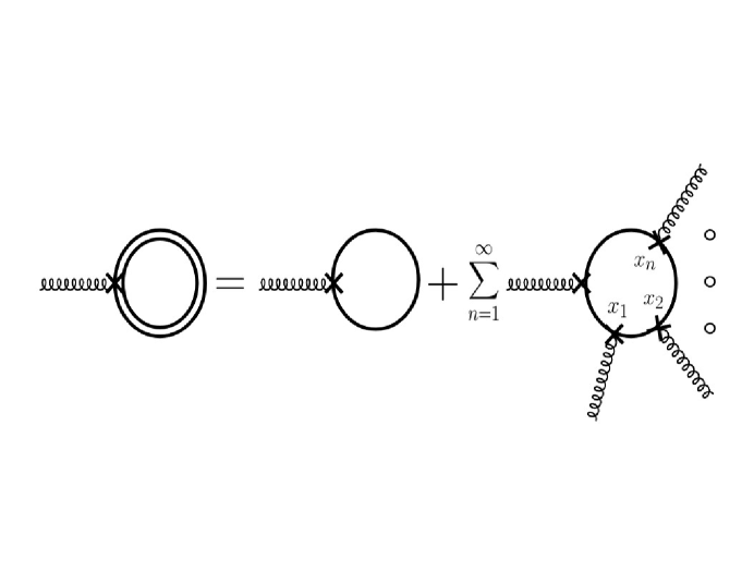
Figure 8: Diagramatic representation of the renormalized energy-momentum tensor in Eqs. (5.32) and (5.39), for which the one-loop correction to the Minkowski vacuum includes resummation over (an even number of) the graviton insertions.

Exponential representation. From Eqs. (7.38), and (3.33–3.34) we infer,

$$\Upsilon(u;u^{\prime})=\cosh^{2}(\tilde{h})-\sinh^{2}(\tilde{h})\left[1-\frac{1}{3}\left(\frac{\omega_{g}\Delta u}{2}\right)^{2}\right]+{\cal O}(\Delta u^{4})\,,\qquad\gamma(u)=1\,,\qquad\;$$ (5.33)

such that,

$$\left[\partial_{u}\partial_{u^{\prime}}\Big{(}\sqrt{\gamma(u)\gamma(u^{\prime})}\Upsilon(u;u^{\prime})\Big{)}^{-1/2}\right]_{u^{\prime}\rightarrow u}=\sinh^{2}(\tilde{h})\frac{\omega_{g}^{2}}{12}\,,\qquad\;$$ (5.34)

and

$${\mathbf{\Upsilon}}^{-1}(u;u)=\left(\!\!\begin{array}[]{ccc}\cosh(\tilde{h})+\sinh(\tilde{h})\cos(\omega_{g}u)&\sinh(\tilde{h})\sin(\omega_{g}u)&0\cdots\cr\sinh(\tilde{h})\sin(\omega_{g}u)&\cosh(\tilde{h})-\sinh(\tilde{h})\cos(\omega_{g}u)&0\cdots\cr 0&0&1\cdots\cr\vdots&\vdots&\!\!\!\!\!\!\vdots\cr\end{array}\!\!\right)\equiv\tilde{g}_{ij}(u)\,,\qquad$$ (5.35)

with $i,j=x,y$ and $\delta_{ij}$ for other values of $i,j$. These results imply that the primitive and renormalized spatial part of the energy-momentum tensor has the identical tensorial form as in (5.11) and (5.12), respectively. The $uu$ component can be read off from Eq. (5.34),

$$\big{[}\partial_{u}\partial_{u^{\prime}}i\Delta_{F}(x;x^{\prime})\big{]}_{x^{\prime}\rightarrow x}\!\! = \!\!\sinh^{2}(\tilde{h})\frac{\omega_{g}^{2}}{12}i\Delta_{F}(x;x)$$ (5.36)

$$= \!\!\sinh^{2}(\tilde{h})\frac{\hbar m^{2}\omega_{g}^{2}}{192\pi^{2}}\left[\frac{2\mu^{D-4}}{D-4}+\ln\Big{(}\frac{m^{2}}{4\pi\mu^{2}}\Big{)}+\gamma_{E}-1\right]$$

$$= \!\!\big{[}\langle\Omega|T^{*}[\hat{T}_{uu}(x)]|\Omega\rangle\big{]}^{(2)}\,.\qquad$$

Keeping in mind the field transformations in Eq. (1.22), $\sinh^{2}(\tilde{h})\rightarrow h^{2}$, we see that the two results differ by a factor $1/(1-h^{2})=1/\gamma(u)$, which is due the fact that, while exponential representation is unimodular, linear representation is not. Nevertheless, the result in Eq. (5.36) is just as in linear representation, proportional to the Einstein tensor, which in exponential representation and for nonpolarized gravitational waves reads (cf. Eq. (5.36)),

$$G_{\mu\nu}=-\frac{\omega_{g}^{2}\sinh^{2}(\tilde{h})}{2}\left(\begin{array}[]{ccccc}1&0&0&\cdots&-1\cr 0&0&0&\cdots&0\cr 0&0&0&\cdots&0\cr\vdots&\vdots&\vdots&\cdots&\vdots\cr-1&0&0&\cdots&1\cr\end{array}\right)\,.$$ (5.37)

Comparing this with Eqs. (5.22) and (5.27–5.32) one sees that the primitive and renormalized energy momentum tensors have the same tensorial form as in linear representation. Therefore, the renormalized result can be summarily written as,

$$\langle\Omega|T^{*}[\hat{T}^{\rm ren}_{\mu\nu}(x)]|\Omega\rangle\!\! = \!\!-\frac{\hbar m^{4}}{64\pi^{2}}\left[\ln\left(\frac{m^{2}}{4\pi\mu^{2}}\right)+\gamma_{E}-\frac{3}{2}\right]g_{\mu\nu}$$ (5.39)

$$\!\!-\frac{\hbar m^{2}}{96\pi^{2}}\left[\log\left(\frac{m^{2}}{4\pi\mu^{2}}\right)+\gamma_{E}-1\right]G_{\mu\nu}\,.\qquad\;$$

Remarkably, this result is both tensorial and representation independent. The result (5.39–5.39) disagrees with Ref. [1], which used Pauli-Villars’ regularization and found that the (gravitational wave contribution to the) renormalized energy-momentum tensor vanishes in the vacuum state.

Polarized gravitational waves.

Linear representation. The calculation for this representation is complicated by the fact that this representation is not unimodular, $\gamma(u)={\rm det}[g_{ij}]=1-h^{2}(u)\neq 1$ ($h^{2}(u)=h_{+}^{2}\cos^{2}(\omega_{g}u-\psi/2)+h_{\times}^{2}\cos^{2}(\omega_{g}u+\psi/2)$). The deformation matrix is of the form,

$$\mathbf{\Upsilon}(u;u^{\prime})\!\! \!\!=\frac{1}{\Delta u}\left[\left(\!\!\begin{array}[]{cc}\int^{u}{\rm d}\bar{u}\frac{1-h_{+}\cos(\omega_{g}\bar{u}-\psi/2)}{\gamma(\bar{u})}&\!-\!\int^{u}{\rm d}\bar{u}\frac{h_{\times}\cos(\omega_{g}\bar{u}+\psi/2)}{\gamma(\bar{u})}\cr\!-\!\int^{u}{\rm d}\bar{u}\frac{h_{\times}\cos(\omega_{g}\bar{u}+\psi/2)}{\gamma(\bar{u})}&\int^{u}{\rm d}\bar{u}\frac{1+h_{+}\cos(\omega_{g}\bar{u}-\psi/2)}{\gamma(\bar{u})}\cr\end{array}\!\!\right)\!\!-\!(u\!\rightarrow\!u^{\prime})\right]\!,\quad$$ (5.42)

and its determinant is denoted by $\Upsilon(u;u^{\prime})$, with $\Upsilon(u;u)=1/\gamma(u)$. Expanding the deformation matrix around $U=(u+u^{\prime})/2$ ($u=U+\Delta u/2,\,u^{\prime}=U-\Delta u/2$) to second order in $\Delta u=u-u^{\prime}$, one obtains,

$$\mathbf{\Upsilon}(u;u^{\prime})\!\! \!\!=\left(\!\!\begin{array}[]{cc}\frac{g_{y}(U)}{\gamma(U)}+\frac{\Delta u^{2}}{24}\left(\frac{g_{y}(U)}{\gamma(U)}\right)^{\prime\prime}&-\frac{g_{xy}(U)}{\gamma(U)}-\frac{\Delta u^{2}}{24}\left(\frac{g_{xy}(U)}{\gamma(U)}\right)^{\prime\prime}\cr-\frac{g_{xy}(U)}{\gamma(U)}-\frac{\Delta u^{2}}{24}\left(\frac{g_{xy}(U)}{\gamma(U)}\right)^{\prime\prime}&\frac{g_{x}(U)}{\gamma(U)}+\frac{\Delta u^{2}}{24}\left(\frac{g_{x}(U)}{\gamma(U)}\right)^{\prime\prime}\cr\end{array}\!\!\right)+{\cal O}(\Delta u^{4})\,,\quad$$ (5.45)

where $g_{x}(U)$, $g_{y}(U)$, and $g_{xy}(U)$ are elements of the metric tensor evaluated at $U$,

$$g^{\perp}_{ij}(U)=\left(\!\begin{array}[]{cc}g_{x}(U)&g_{xy}(U)\cr g_{xy}(U)&g_{y}(U)\cr\end{array}\!\right)\,,\qquad g_{{}_{x}\atop{}^{y}}(U)=1\pm h_{+}\cos(\omega_{g}U-\psi/2)\,,\quad g_{xy}=h_{\times}\cos(\omega_{g}U+\psi/2)\,,$$ (5.46)

such that $g_{x}(U)g_{y}(U)-g_{xy}(U)^{2}=\gamma(U)$.

Note first that Eq. (5.45) implies, $\left[{\mathbf{\Upsilon}}^{-1}(u;u)\right]_{ij}=g_{ij}^{\perp}(u)$ (cf. Eqs. (5.16) and (5.35)), from which we immediately conclude that, after the renormalization is exacted, one obtains the first part of the energy-momentum in the tensorial form as in Eq. (5.39).

Next, upon inserting Eq. (5.45) into $\Upsilon(u;u^{\prime})=\Upsilon_{x}(u;u^{\prime})\Upsilon_{y}(u;u^{\prime})-\Upsilon_{xy}(u;u^{\prime})^{2}$ yields,

$$\Upsilon(u;u^{\prime})\!\! = \!\!\frac{1}{\gamma}+\frac{\Delta u^{2}}{24}\left(\frac{g_{x}g_{y}^{\prime\prime}\!+\!g_{y}g_{x}^{\prime\prime}\!-\!2g_{xy}g_{xy}^{\prime\prime}}{\gamma^{2}}\!-\!2\frac{\gamma\gamma^{\prime\prime}\!-\!\gamma^{\prime 2}}{\gamma^{3}}\right)$$ (5.47)

$$+ \!\!{\cal O}(\Delta u^{4})\,,\quad$$

where for notational brevity, in Eq. (5.47) and in what follows, we suppressed the dependence on $U$. Multiplying this by,

$$\sqrt{\gamma(u)\gamma(u^{\prime})}=\gamma+\frac{\Delta u^{2}}{8}\frac{\gamma^{\prime 2}\!-\!\gamma\gamma^{\prime\prime}}{\gamma^{3}}+{\cal O}(\Delta u^{4})\,,$$ (5.48)

yields,

$$\sqrt{\gamma(u)\gamma(u^{\prime})}\Upsilon(u;u^{\prime})\!\! = \!\!1+\frac{\Delta u^{2}}{24}\left(\frac{g_{x}g_{y}^{\prime\prime}\!+\!g_{y}g_{x}^{\prime\prime}\!-\!2g_{xy}g_{xy}^{\prime\prime}}{\gamma}\!+\!\frac{\gamma\gamma^{\prime\prime}\!-\!\gamma^{\prime 2}}{\gamma^{2}}\right)$$ (5.49)

$$+ \!\!{\cal O}(\Delta u^{4})\,,\quad$$

from which it is easy to obtain,

$$\left[\partial_{u}\partial_{u^{\prime}}\Big{(}\sqrt{\gamma(u)\gamma(u^{\prime})}\Upsilon(u;u^{\prime})\Big{)}^{-1/2}\,\right]_{u^{\prime}\rightarrow u}\!\! = \!\!\frac{1}{24}\left(\frac{g_{x}g_{y}^{\prime\prime}\!+\!g_{y}g_{x}^{\prime\prime}\!-\!2g_{xy}g_{xy}^{\prime\prime}}{\gamma}\!+\!\frac{\gamma\gamma^{\prime\prime}\!-\!\gamma^{\prime 2}}{\gamma^{2}}\right)\,,\qquad\;$$ (5.50)

where the primes denote derivatives with respect to $u$ and we made use of, $\partial_{u}\partial_{u^{\prime}}=\frac{1}{4}\partial_{U}^{2}-\partial^{2}_{\Delta u}$. Inserting Eq. (5.50) into Eq. (5.1) results in,

$$\big{[}\langle\Omega|T^{*}[\hat{T}_{uu}(x)]|\Omega\rangle\big{]}^{(2)}\!\!\! = \!\!\!\big{[}\partial_{u}\partial_{u^{\prime}}i\Delta_{F}(x;x^{\prime})\big{]}_{x^{\prime}\rightarrow x}=\frac{1}{24}\left(\frac{g_{x}g_{y}^{\prime\prime}\!+\!g_{y}g_{x}^{\prime\prime}\!-\!2g_{xy}g_{xy}^{\prime\prime}}{\gamma}\!+\!\frac{\gamma\gamma^{\prime\prime}\!-\!\gamma^{\prime 2}}{\gamma^{2}}\right)i\Delta_{F}(x;x)\,,\qquad\;\;\;$$ (5.51)

from where one obtains the second contribution to the energy-momentum tensor, which in Cartesian coordinates reads,

$$\big{[}\langle\Omega|T^{*}[\hat{T}_{\mu\nu}(x)]|\Omega\rangle\big{]}^{(2)}\!\! = \!\!\frac{\hbar m^{2}}{384\pi^{2}}\left(\frac{g_{x}g_{y}^{\prime\prime}\!+\!g_{y}g_{x}^{\prime\prime}\!-\!2g_{xy}g_{xy}^{\prime\prime}}{\gamma}\!+\!\frac{\gamma\gamma^{\prime\prime}\!-\!\gamma^{\prime 2}}{\gamma^{2}}\right)$$ (5.57)

$$\!\!\hskip 0.0pt\times\;\left[\frac{2\mu^{D-4}}{D-4}\!+\!\ln\Big{(}\frac{m^{2}}{4\pi\mu^{2}}\Big{)}\!+\!\gamma_{E}\!-\!1\right]\left(\begin{array}[]{ccccc}1&0&0&\cdots&-1\cr 0&0&0&\cdots&0\cr 0&0&0&\cdots&0\cr\vdots&\vdots&\vdots&\cdots&\vdots\cr-1&0&0&\cdots&1\cr\end{array}\right).\qquad\;\;\;$$

The next step is to calculate the Einstein tensor, which one can show to be of the form,

$$G_{\mu\nu}(u)=-\frac{1}{4}\left(\frac{g_{x}g_{y}^{\prime\prime}\!+\!g_{y}g_{x}^{\prime\prime}\!-\!2g_{xy}g_{xy}^{\prime\prime}}{\gamma}\!+\!\frac{\gamma\gamma^{\prime\prime}\!-\!\gamma^{\prime 2}}{\gamma^{2}}\right)\left(\begin{array}[]{ccccc}1&0&0&\cdots&-1\cr 0&0&0&\cdots&0\cr 0&0&0&\cdots&0\cr\vdots&\vdots&\vdots&\cdots&\vdots\cr-1&0&0&\cdots&1\cr\end{array}\right)\,.$$ (5.58)

This is proportional to Eq. (5.57), and therefore the energy-momentum tensor in Eq. (5.57) can be renormalized by the Hilbert-Einstein counterterm (5.23–5.24). Upon choosing the bare Newton constant as in Eq. (5.26) and adding the corresponding energy-momentum tensor (5.24) to Eq. (5.57) renormalizes the energy-momentum tensor, such that one again obtains the renormalized one-loop energy momentum tensor in the tensorial form given in Eqs. (5.39–5.39).

Exponential representation. In this representation the deformation matrix is of the form,

$$\hskip-8.5359pt\mathbf{\Upsilon}(u;u^{\prime})$$ (5.59)

$$\!\!=\frac{1}{\Delta u}\left[\left(\!\!\begin{array}[]{cc}\int^{u}{\rm d}\bar{u}\left(\cosh(\tilde{h}(\bar{u}))\!-\!\frac{\sinh(\tilde{h}(\bar{u}))}{\tilde{h}(\bar{u})}h_{+}c_{+}(\bar{u})\right)&\!-\!\int^{u}{\rm d}\bar{u}\frac{\sinh(\tilde{h}(\bar{u}))}{\tilde{h}(\bar{u})}h_{\times}c_{\times}(\bar{u})\cr\!-\!\int^{u}{\rm d}\bar{u}\frac{\sinh(\tilde{h}(\bar{u}))}{\tilde{h}(\bar{u})}h_{\times}c_{\times}(\bar{u})&\int^{u}{\rm d}\bar{u}\left(\cosh(\tilde{h}(\bar{u}))\!+\!\frac{\sinh(\tilde{h}(\bar{u}))}{\tilde{h}(\bar{u})}h_{+}c_{+}(\bar{u})\right)\cr\end{array}\!\!\right)\!\!-\!(u\!\rightarrow\!u^{\prime})\right]\!,\quad$$ (5.62)

where $\tilde{h}^{2}(u)=\tilde{h}_{+}^{2}c_{+}^{2}(u)+\tilde{h}_{\times}^{2}c_{\times}^{2}(u)$, see Eqs. (1.11–1.12), and the determinant is denoted by $\Upsilon(u;u^{\prime})$, with $\Upsilon(u;u)=1$.

Upon denoting elements of the metric tensor in the $xy-$plane (cf. Eq. (1.10) and (1.16)) as,

$$g_{ij}^{\perp}(u)\equiv\left(\!\!\begin{array}[]{cc}g_{x}(u)&g_{xy}(u)\cr g_{xy}(u)&g_{y}(u)\cr\end{array}\!\!\right)\,,\qquad g_{{}_{x}\atop{}^{y}}=\cosh(\tilde{h})\mp\frac{\sinh(\tilde{h})}{\tilde{h}}h_{+}c_{+}\,,\quad g_{xy}=\frac{\sinh(\tilde{h})}{\tilde{h}}h_{\times}c_{\times}\,,\quad$$ (5.63)

one obtains that the structure of the deformation matrix $\mathbf{\Upsilon}$ is identical as in Eq. (5.47), but with the simplification, $\gamma(u)=1$. With these remarks in mind the calculation of the energy-momentum tensor, the Einstein tensor and renormalization proceeds as in the above subsection on linear representation, but with $\gamma\rightarrow 1$ and $\gamma^{\prime}\rightarrow 0$, resulting again in the renormalized energy-momentum tensor in Eqs. (5.39–5.39).

The energy-momentum tensor in Eq. (5.39) is proportional to the (classical) backreaction of gravitational waves,  which induces a backreaction, $T^{\rm gw}_{\mu\nu}(x)=-G_{\mu\nu}(x)/(8\pi G)$ (see Eq. (5.24)). Comparing this with Eq. (5.39) one obtains, 

$$\frac{T^{\rm 1\,loop\;scalar\;gw}_{\mu\nu}}{T^{\rm gw}_{\mu\nu}}=\frac{G\hbar m^{2}}{12\pi}\log\left(\frac{m^{2}}{4\pi\bar{\mu}^{2}}\right)\,,$$ (5.65)

where $\bar{\mu}^{2}=\mu^{2}{\rm e}^{1-\gamma_{E}}$, which is suppressed as, $\sim m^{2}/m_{\rm P}^{2}$ ($m_{\rm P}^{2}=\hbar/G$). This implies that: the larger is the scalar mass, the stronger is the gravitational backreaction. In particular, the backreaction vanishes in the massless scalar limit. Such a matter backreaction can be used in controlled environments to detect very heavy scalar particles, whose presence could not be detected by other means.

Even though the result in (5.39) contains a directional flow of energy, we expect it to hold in more general situations, such as multifrequency gravitational waves and stochastic gravitational backgrounds, for which the energy-momentum tensor induced by gravitational waves, $T_{\mu\nu}^{\rm gw}$, has a perfect relativistic fluid form, which is in the fluid rest frame diagonal, $[T_{\mu}^{\;\nu}]^{\rm gw}={\rm diag}(\rho_{\rm gw},{\cal P}_{\rm gw},{\cal P}_{\rm gw},{\cal P}_{\rm gw})$, and characterized by the energy momentum tensor $\rho_{\rm gw}$ and by the isotropic pressures, ${\cal P}_{\rm gw}$, of the form, ${\cal P}_{\rm gw}=w_{\rm gw}\rho_{\rm gw}$, with the equation of state parameter, $w_{\rm gw}=1/3$.

6 Conclusions and outlook

In this paper we construct the massive real scalar field propagator for classical, planar gravitational waves propagating on the Minkowski background. Our principal results are in section 3, where the Wightman functions (3.11) and the propagator (3.25–3.26) in general $D$ spacetime dimensions are constructed. The solutions differ from the corresponding Minkowski vacuum two-point functions in two aspects:

1. Gravitational waves change the strength of scalar field fluctuations, and its impact is reflected by the prefactor in Eq. (3.11);

2. The Minkowski Poincaré invariant distance function is changed into the deformed, non-local, Lorentz symmetry-breaking, distance function in Eqs. (3.14–3.17).

In this work, we construct the two-point functions only for monochromatic gravitational waves moving in a definite direction, i.e. planar gravitational waves. However, we consider both nonpolarized and polarized gravitational waves (for which the amplitudes of the $(+)$ and $(\times)$ polarizations differ and/or the difference in phases of the two polarizations is not $\pi/2$). In Appendix D we show how to generalize to $D(D-3)/2$ polarization, which exist in $D$ spacetime dimensions. This work focuses on monochromatic gravitational waves. However, generalization to more general wave forms (as observed in realistic systems [9, 10]) is feasible, and we leave that for future work. Our two-point functions resum all powers of gravitational strain, and thus allow to study both linear and non-linear effects. To prevent interpretational ambiguities of the results that may occur at higher orders in the gravitational strain, we use two inequivalent field representations for gravitational waves – which we dub linear representation (1.2–1.3) and exponential representation (1.6), (1.16), which allows one to study how physical observables depend on the representation used.

This has borne fruit in sections 4 and 5, where we consider simple one-loop applications. In section 4 we construct the renormalized one-loop effective action (4.12), and show that it does not get affected by planar gravitational waves. The analogous result holds true for the one-loop mass (4.15) induced by the scalar self-interaction. In section 5 we construct the renormalized one-loop energy-momentum tensor induced by the scalar field fluctuations. Our results (5.39–5.39) show that the quantum scalar backreaction induced by the planar gravitational waves harbors two distinct contributions:

1. The contribution (5.39), which is proportional to the metric tensor $g_{\mu\nu}$ and thus contributes to the energy-momentum tensor as the cosmological constant. Notice that this contribution also depends on the gravitational wave strain through the metric tensor $g_{\mu\nu}$.

2. The contribution (5.39), which is proportional to the Einstein tensor induced by the gravitational waves. The leading order contribution is quadratic in the gravitational wave strain, however our calculation resums all powers of the gravitational wave strain.

The energy-momentum tensor (5.39–5.39) is tensorial, which gives us confidence that the results are correct.

This work assumes single frequency (monochromatic) waves moving in a definite direction. In more realistic situations however, one expects that the gravitational waves carry higher frequency overtones,  and – if generated by multiple sources – they will move in different directions, an important example being the stochastic gravitational wave background generated by cosmic inflation. Constructing the propagator for such more general gravitational wave backgrounds is a pursuit worth the effort.

While the initial results presented in this work represent simple applications, we emphasise that our propagator constitutes an essential ingredient for understanding the important question, namely how matter fields respond to classical gravitational waves in the context of interacting quantum field theories. While this paper discusses the massive real scalar field, we expect that generalization to matter fields with spin is feasible by making use of the techniques established in this work.

7 Appendices

Appendix A: Propagator integral

In this appendix we construct the Wightman functions and the propagator by writing them as a power-series in multipoles by expanding the phase in the exponential induced by the gravitational waves in powers of spatial derivatives. The general form of the expansion for the Wightman functions (3.9–3.10) is,

$$i\Delta^{(+)}(x;x^{\prime})\!\! = \!\!\sum_{n=0}^{\infty}\frac{i^{n}}{n!}\left[\Delta\Psi_{0}(u;u^{\prime})(\partial_{x}^{2}\!+\!\partial_{y}^{2})\!+\!\Delta\Psi_{+}(u;u^{\prime})(\partial_{x}^{2}\!-\!\partial_{y}^{2})\!+\!\Delta\Psi_{\times}(u;u^{\prime})\partial_{x}\partial_{y}\right]^{n}\!\frac{i\Delta_{n}^{(+)}(x;x^{\prime})}{\left[\gamma(u)\gamma(u^{\prime})\right]^{\frac{1}{4}}},\qquad\;$$ (7.1)

$$i\Delta^{(-)}(x;x^{\prime})\!\! = \!\!\sum_{n=0}^{\infty}\frac{i^{n}}{n!}\left[\Delta\Psi_{0}(u;u^{\prime})(\partial_{x}^{2}\!+\!\partial_{y}^{2})\!+\!\Delta\Psi_{+}(u;u^{\prime})(\partial_{x}^{2}\!-\!\partial_{y}^{2})\!+\!2\Delta\Psi_{\times}(u;u^{\prime})\partial_{x}\partial_{y}\right]^{n}\!\frac{i\Delta_{n}^{(-)}(x;x^{\prime})}{\left[\gamma(u)\gamma(u^{\prime})\right]^{\frac{1}{4}}},\qquad\;$$ (7.2)

where $\gamma(u)={\rm det}[g_{ij}]$ is the determinant of the spatial metric, which differs from unity in linear representation (for example, $\gamma(u)=1-h^{2}$ for nonpolarized waves), but in exponential representation, $\gamma(u)=1$, and can be omitted. Eqs. (7.1–7.2) are obtained by expanding the mode functions (3.7) in Eqs. (3.9–3.10) in powers of $\Psi(u)$.

Linear representation. For nonpolarized gravitational waves in linear representation (1.2) from Eq. (3.7) one obtains,

$$\Delta\Psi_{0}(u;u^{\prime})\!\! = \!\!\Psi_{0}(u)-\Psi_{0}(u^{\prime})\,,\qquad\;\;\Psi_{0}(u)=\frac{h^{2}}{1-h^{2}}u$$

$$\Delta\Psi_{+}(u;u^{\prime})\!\! = \!\!\Psi_{+}(u)-\Psi_{+}(u^{\prime})\,,\qquad\Psi_{+}(u)=-\frac{h_{+}\sin(\omega_{g}u)}{\omega_{g}(1\!-\!h^{2})}$$

$$\Delta\Psi_{\times}(u;u^{\prime})\!\! = \!\!\Psi_{\times}(u)-\Psi_{\times}(u^{\prime})\,,\qquad\Psi_{\times}(u)=\frac{h_{\times}\cos(\omega_{g}u)}{\omega_{g}(1\!-\!h^{2})}\,.$$ (7.3)

For singly polarized gravitational waves, $h_{+}\neq 0$ and $h_{\times}=0$, one can easily read off from Eq. (3.44) the phase functions,

$$\Psi_{0}(u)\!\! = \!\!\frac{1}{\omega_{g}}\frac{1}{\sqrt{1\!-\!h_{+}^{2}}}\bigg{\{}\text{arctan}\bigg{[}\sqrt{\frac{1\!-\!h_{+}}{1\!+\!h_{+}}}\tan\Big{(}\frac{\omega_{g}u}{2}\Big{)}\bigg{]}\!+\!\text{arctan}\bigg{[}\sqrt{\frac{1\!+\!h_{+}}{1\!-\!h_{+}}}\tan\Big{(}\frac{\omega_{g}u}{2}\Big{)}\bigg{]}\bigg{\}}-u\,,$$

$$\Psi_{+}(u)\!\! = \!\!\frac{1}{\omega_{g}}\frac{1}{\sqrt{1\!-\!h_{+}^{2}}}\bigg{\{}\text{arctan}\bigg{[}\sqrt{\frac{1\!-\!h_{+}}{1\!+\!h_{+}}}\tan\Big{(}\frac{\omega_{g}u}{2}\Big{)}\bigg{]}\!-\!\text{arctan}\bigg{[}\sqrt{\frac{1\!+\!h_{+}}{1\!-\!h_{+}}}\tan\Big{(}\frac{\omega_{g}u}{2}\Big{)}\bigg{]}\bigg{\}}\,,$$

$$\Psi_{\times}(u)\!\! = \!\!0\,.$$ (7.4)

On the other hand, when $h_{\times}\neq 0$ and $h_{+}=0$, from Eq. (3.45) one infers,

$$\Psi_{0}(u)\!\! = \!\!\frac{1}{\omega_{g}\sqrt{1\!-\!h_{\times}^{2}}}\text{arctan}\bigg{[}\frac{1}{\sqrt{1\!-\!h_{\times}^{2}}}\tan(\omega_{g}u)\bigg{]}-u\,,$$

$$\Psi_{+}(u)\!\! = \!\!0\,,$$

$$\Psi_{\times}(u)\!\! = \!\!-\,\frac{1}{\omega_{g}\sqrt{1\!-\!h_{\times}^{2}}}\text{arctan}\bigg{[}\frac{h_{\times}}{\sqrt{1\!-\!h_{\times}^{2}}}\sin(\omega_{g}u)\bigg{]}\,.$$ (7.5)

For general polarized gravitational waves one can extract the phase functions from Eqs. (3.47–3.48),

$$\Psi_{0}(u)\!\! = \!\!\frac{1}{\omega_{g}\sqrt{1-(h_{+}^{2}+h_{\times}^{2})+h_{+}^{2}h_{\times}^{2}s_{\psi}^{2}}}\text{Arctan}\Bigg{(}\frac{h_{\times}^{2}s_{\psi}c_{\psi}+[1-h_{\times}^{2}s_{\psi}^{2}]\tan(\omega_{g}u-\frac{\psi}{2})}{\sqrt{1-(h_{+}^{2}+h_{\times}^{2})+h_{+}^{2}h_{\times}^{2}s_{\psi}^{2}}}\Bigg{)}-u\,,$$ (7.6)

$$\Psi_{+}(u)\!\! = \!\!\frac{1}{\omega_{g}\sqrt{1-(h_{+}^{2}+h_{\times}^{2})+h_{+}^{2}h_{\times}^{2}s_{\psi}^{2}}}$$ (7.7)

$$\times \!\!\left[\frac{ih_{+}(1-h_{\times}^{2}s_{\psi}^{2})\text{Arctanh}[g(u)]}{2\sqrt{h_{+}^{2}+h_{\times}^{2}-h_{\times}^{2}s_{\psi}^{2}(2+h_{+}^{2}+h_{\times}^{2})-2ih_{\times}^{2}c_{\psi}s_{\psi}\sqrt{1-(h_{+}^{2}+h_{\times}^{2})+h_{+}^{2}h_{\times}^{2}s_{\psi}^{2}}}}+{\rm c.c.}\right]\,,$$

$$\Psi_{\times}(u)\!\! = \!\!\frac{1}{\omega_{g}\sqrt{1-(h_{+}^{2}+h_{\times}^{2})+h_{+}^{2}h_{\times}^{2}s_{\psi}^{2}}}$$ (7.8)

$$\times \!\!\left[\frac{i\big{[}\!-h_{\times}^{3}s_{\psi}^{2}c_{\psi}\!+\!ih_{\times}s_{\psi}\sqrt{1\!-\!(h_{+}^{2}\!+\!h_{\times}^{2})\!+\!h_{+}^{2}h_{\times}^{2}s_{\psi}^{2}}\!-\!h_{\times}c_{\psi}(1\!-\!h_{\times}^{2}s_{\psi}^{2})\big{]}\text{Arctanh}[g(u)]}{2\sqrt{h_{+}^{2}+h_{\times}^{2}-h_{\times}^{2}s_{\psi}^{2}(2\!+\!h_{+}^{2}\!+\!h_{\times}^{2})\!-\!2ih_{\times}^{2}c_{\psi}s_{\psi}\sqrt{1\!-\!(h_{+}^{2}\!+\!h_{\times}^{2})\!+\!h_{+}^{2}h_{\times}^{2}s_{\psi}^{2}}}}+{\rm c.c.}\right]\,.\qquad\;\;$$

This result is complicated, nevertheless its correctness can be checked by considering the simpler limits when either $h_{\times}=0$ or $h_{+}=0$ vanishes. For example, in the $(+)-$polarized case Eqs. (7.6–7.8) imply,

$$\Psi(u)\!\! = \!\!-(k_{x}^{2}+k_{y}^{2})u+\frac{k_{x}^{2}+k_{y}^{2}}{\omega_{g}\sqrt{1\!-\!h_{+}^{2}}}\text{Arctan}\Bigg{[}\frac{\tan(\omega_{g}u)}{\sqrt{1-h_{+}^{2}}}\Bigg{]}+\frac{k_{y}^{2}\!-\!k_{x}^{2}}{\omega_{g}\sqrt{1\!-\!h_{+}^{2}}}$$

$$\times \!\!\!\Bigg{\{}\!\!-\frac{i}{2}\text{Arctanh}\Bigg{[}\!\frac{\cos(\omega_{g}u)+i\sqrt{1\!-\!h_{+}^{2}}\sin(\omega_{g}u)}{h_{+}}\!\Bigg{]}\!+\!\frac{i}{2}\text{Arctanh}\Bigg{[}\!\frac{\cos(\omega_{g}u)-i\sqrt{1\!-\!h_{+}^{2}}\sin(\omega_{g}u)}{h_{+}}\!\Bigg{]}\!\Bigg{\}}\,.\;\;$$

Even though the form of (Appendix A: Propagator integral) does not match (3.44), one can show they are identical on the interval $-\frac{\pi}{2}<\omega_{g}u<\frac{\pi}{2}$. The equivalence on broader domains can be reestablished by analytically extending Eqs. (7.6–7.8) in analogous manner as it was done in the case of single polarizations in Eqs. (3.44) and (3.45).

Exponential representation. For nonpolarized gravitational waves in exponential representation one obtains from Eq. (3.32),

$$\Delta\Psi_{0}(u;u^{\prime})\!\! = \!\!\Psi_{0}(u)-\Psi_{0}(u^{\prime})\,,\qquad\Psi_{0}(u)=(\cosh(\tilde{h})\!-\!1)u\,,$$

$$\Delta\Psi_{\times}(u;u^{\prime})\!\! = \!\!\Psi_{+}(u)-\Psi_{+}(u^{\prime})\,,\qquad\Psi_{+}(u)=-\sinh(\tilde{h})\frac{\sin(\omega_{g}u)}{\omega_{g}}\,,$$

$$\Delta\Psi_{\times}(u;u^{\prime})\!\! = \!\!\Psi_{\times}(u)-\Psi_{\times}(u^{\prime})\,,\qquad\Psi_{\times}(u)=\sinh(\tilde{h})\frac{\cos(\omega_{g}u)}{\omega_{g}}\,.\qquad\;\;$$ (7.10)

The integrals for polarized gravitational waves in exponential representation cannot be evaluated in terms of known functions, and for that reason we do not separately consider singly polarized cases. In the general case from Eq. (3.54) one can extract the phase functions in Eqs. (7.1–7.2), 

$$\Psi_{0}(u)\!\! = \!\!\int^{u}{\rm d}\bar{u}\big{(}\!\cosh(\tilde{h}(\bar{u}))\!-\!1\big{)}\,,\hskip 14.22636pt$$ (7.13)

$$\Psi_{+}(u)\!\! = \!\!-\int^{u}{\rm d}\bar{u}\frac{\sinh(\tilde{h}(\bar{u}))}{\tilde{h}(\bar{u})}\tilde{h}_{+}c_{+}(\bar{u})\,,\hskip 14.22636pt$$ (7.14)

$$\Psi_{\times}(u)\!\! = \!\!-\int^{u}{\rm d}\bar{u}\frac{\sinh(\tilde{h}(\bar{u}))}{\tilde{h}(\bar{u})}\tilde{h}_{\times}c_{\times}(\bar{u})\,,\hskip 14.22636pt$$ (7.15)

with $\tilde{h}(\bar{u})=\sqrt{\tilde{h}_{+}^{2}c_{+}^{2}(\bar{u})+\tilde{h}_{\times}^{2}c_{\times}^{2}(\bar{u})}$. However, the integrals do simplify if one expands the original exponential representation (1.6) in powers of $\tilde{h}_{+}$ and $\tilde{h}_{\times}$, as it was done in Eqs. (3.56–3.70),

$$\Psi_{0}(u)\!\! = \!\!\frac{1}{4}\left(\tilde{h}_{+}^{2}+\tilde{h}_{\times}^{2}\right)u+\frac{\tilde{h}_{+}^{2}}{8\omega_{g}}\sin\left(2\omega_{g}u-\psi\right)+\frac{\tilde{h}_{\times}^{2}}{8\omega_{g}}\sin\left(2\omega_{g}u+\psi\right)+{\cal O}\big{(}\tilde{h}_{+}^{4},\tilde{h}_{+}^{2}\tilde{h}_{\times}^{2},\tilde{h}_{\times}^{4}\big{)}\,,\hskip 25.6073pt$$ (7.16)

$$\Psi_{+}(u)\!\! = \!\!-\frac{\tilde{h}_{+}}{\omega_{g}}\sin\left(\omega_{g}u-\frac{\psi}{2}\right)+{\cal O}\big{(}\tilde{h}_{+}^{3},\tilde{h}_{+}\tilde{h}_{\times}^{2}\big{)}\,,\hskip 14.22636pt$$ (7.17)

$$\Psi_{\times}(u)\!\! = \!\!-\frac{\tilde{h}_{\times}}{\omega_{g}}\sin\left(\omega_{g}u+\frac{\psi}{2}\right)+{\cal O}\big{(}\tilde{h}_{+}^{2}\tilde{h}_{\times},\tilde{h}_{\times}^{3}\big{)}\,.\hskip 14.22636pt$$ (7.18)

Wightman functions and propagator. The biscalars $i\Delta_{n}^{(\pm)}(x;x^{\prime})$ in (7.1) and (7.2) denote the integrals in Eqs (3.9–3.10),

$$i\Delta_{n}^{(+)}(x;x^{\prime})\!\! \equiv \!\!\int\frac{{\rm d}^{D-1}k}{(2\pi)^{D-1}}\frac{\hbar}{2\omega[2\Omega_{-}]^{n}}\exp\left\{i\vec{k}_{\perp}\!\cdot\Delta\vec{x}_{\perp}-\frac{i}{2}\Big{[}\Omega_{-}(\vec{k})\Delta v+\Omega_{+}(\vec{k})\Delta u\Big{]}\right\}\qquad$$ (7.19)

$$i\Delta_{n}^{(-)}(x;x^{\prime})\!\! = \!\!\int\frac{{\rm d}^{D-1}k}{(2\pi)^{D-1}}\frac{\hbar}{2\omega[2\Omega_{-}]^{n}}\exp\left\{-i\vec{k}_{\perp}\!\cdot\Delta\vec{x}_{\perp}+\frac{i}{2}\Big{[}\Omega_{-}(\vec{k})\Delta v+\Omega_{+}(\vec{k})\Delta u\Big{]}\right\}$$ (7.20)

where $n=0,1,2,\cdots$ is an integer, $\Delta\vec{x}_{\perp}=\vec{x}_{\perp}\!-\!\vec{x}_{\perp}^{\,\prime}$, $\Delta u=u\!-\!u^{\prime}$, $\Delta v=v\!-\!v^{\prime}$. The form of the integrals in (7.19–7.20) follows from expanding the phases of the mode functions in (3.7) in powers of $\Psi(u)$. Recall that $i\Delta_{n}^{(+)}(x;x)=\big{[}i\Delta_{n}^{(-)}(x;x^{\prime})\big{]}^{*}$ such that it suffices to evaluate $i\Delta_{n}^{(+)}(x;x)$.

Next, by making use of $\Omega_{\pm}(\vec{k})=\omega_{\perp}^{2}/\Omega_{\mp}(\vec{k})$ ($\omega_{\perp}=\sqrt{k_{\perp}^{2}+m^{2}}$, $k_{\perp}\equiv\|\vec{k}_{\perp}\|$) and $\int_{-\infty}^{\infty}{\rm d}k^{D-1}=\int_{0}^{\infty}{\rm d}\Omega_{+}(\omega/\Omega_{+})$, the integral (7.19) becomes,

$$i\Delta_{n}^{(+)}=\frac{\hbar}{2(2\pi)^{D-1}}\int\frac{{\rm d}^{D-2}k_{\perp}}{\omega_{\perp}^{2n}}{\rm e}^{i\vec{k}_{\perp}\cdot\Delta\vec{x}_{\perp}}\int_{0}^{\infty}{\rm d}\Omega_{+}\frac{\Omega_{+}^{n-1}}{2^{n}}\exp\Big{\{}\!-\frac{i}{2}\Big{[}\Omega_{+}\Delta u+\frac{\omega_{\perp}^{2}}{\Omega_{+}}\Delta v\Big{]}\Big{\}}\,,\qquad(n=0,1,2,\cdots)\,.$$ (7.21)

The $\Omega_{+}$-integral can be performed with the help of Eq. (3.471.9) in Ref. [16] resulting in,

$$i\Delta_{n}^{(+)}=\frac{\hbar}{(2\pi)^{D-1}}\int\frac{{\rm d}^{D-2}k_{\perp}}{\omega_{\perp}^{2n}}\,{\rm e}^{i\vec{k}_{\perp}\cdot\Delta\vec{x}_{\perp}}\left[\frac{\omega_{\perp}}{2}\sqrt{\frac{\Delta v\!-\!i\epsilon}{\Delta u\!-\!i\epsilon}}\,\right]^{n}K_{n}\big{(}\omega_{\perp}\sqrt{\!-(\Delta u\!-\!i\epsilon)(\Delta v\!-\!i\epsilon)}\,\big{)}\,.\qquad$$ (7.22)

The origin of the $i\epsilon$ prescriptions in (7.22) is in the requirement on convergence of the integral (7.21). Namely, convergence in the limit when $\Omega_{+}\rightarrow+\infty$ requires $\Delta u\rightarrow\Delta u-i\epsilon$, and when $\Omega_{+}\rightarrow 0$ it requires $\Delta v\rightarrow\Delta v-i\epsilon$.

Next we rewrite the $\vec{k}_{\perp}-$integral in (7.22) in polar coordinates,

$$\int{\rm d}^{D-2}k_{\perp}{\rm e}^{i\vec{k}_{\perp}\cdot\Delta\vec{x}_{\perp}}\!\! = \!\!\int_{0}^{\infty}{\rm d}k_{\perp}k_{\perp}^{D-3}\int{\rm d}\Omega_{D-4}\int_{0}^{\pi}{\rm d}\theta\,{\rm e}^{ik_{\perp}\|\Delta\vec{x}_{\perp}\|\cos(\theta)}\big{[}\!\sin(\theta)\big{]}^{D-4}$$ (7.23)

$$= \!\!(2\pi)^{(D-2)/2}\int_{0}^{\infty}{\rm d}k_{\perp}k_{\perp}^{D-3}\times\frac{J_{\frac{D-4}{2}}\big{(}k_{\perp}\|\Delta\vec{x}_{\perp}\|\big{)}}{(k_{\perp}\|\Delta\vec{x}_{\perp}\|)^{\frac{D-4}{2}}}\,,$$

where $\int{\rm d}\Omega_{D-4}=2\pi^{(D-3)/2}/\Gamma\big{(}\tfrac{D-3}{2}\big{)}$ is the volume of the $(D-4)-$dimensional sphere and we made use of Eq. (8.411.7) from Ref. [16]. With this Eq. (7.22) becomes,

$$i\Delta_{n}^{(+)}=\frac{\hbar}{(2\pi)^{\frac{D}{2}}}\left[\frac{1}{2}\sqrt{\frac{\Delta v\!-\!i\epsilon}{\Delta u\!-\!i\epsilon}}\,\right]^{n}\!\!\frac{1}{\|\Delta\vec{x}_{\perp}\|^{\frac{D-4}{2}}}\int_{0}^{\infty}\!{\rm d}k_{\perp}k_{\perp}^{\frac{D-2}{2}}J_{\frac{D-4}{2}}\big{(}k_{\perp}\|\Delta\vec{x}_{\perp}\|\big{)}\frac{K_{n}\big{(}\omega_{\perp}\sqrt{-(\Delta u\!-\!i\epsilon)(\Delta v\!-\!i\epsilon)}\,\big{)}}{\omega_{\perp}^{n}}\,,\quad$$ (7.24)

with $\omega_{\perp}=\sqrt{k_{\perp}^{2}+m^{2}}$. The last integral can be evaluated by using (6.596.7) in Ref. [16], which gives,

$$\hskip-28.45274pt\int_{0}^{\infty}\!{\rm d}k_{\perp}k_{\perp}^{\frac{D-2}{2}}J_{\frac{D-4}{2}}\big{(}k_{\perp}\|\Delta\vec{x}_{\perp}\|\big{)}\frac{K_{n}\big{(}\omega_{\perp}\sqrt{-(\Delta u\!-\!i\epsilon)(\Delta v\!-\!i\epsilon)}\,\big{)}}{\omega_{\perp}^{n}}$$

$$\hskip 28.45274pt=\frac{\|\Delta\vec{x}_{\perp}\|^{\frac{D-4}{2}}}{\left[\sqrt{-(\Delta u\!-\!i\epsilon)(\Delta v\!-\!i\epsilon)}\right]^{n}}\left(\frac{\sqrt{\!-(\Delta u\!-\!i\epsilon)(\Delta v\!-\!i\epsilon)\!+\!\|\Delta\vec{x}_{\perp}\|^{2}}}{m}\,\right)^{n-\frac{D-2}{2}}$$

$$\hskip 170.71652pt\times\,K_{n-\frac{D-2}{2}}\big{(}m\sqrt{\!-(\Delta u\!-\!i\epsilon)(\Delta v\!-\!i\epsilon)\!+\!\|\Delta\vec{x}_{\perp}\|^{2}}\,\big{)}\,.\quad$$ (7.25)

Inserting this into (7.24) yields,

$$i\Delta_{n}^{(+)}(x;x^{\prime})\!\!\! = \!\!\frac{\hbar m^{D-2-n}}{(2\pi)^{D/2}}\left[\frac{-1}{2m(\Delta u\!-\!i\epsilon)}\,\right]^{n}\!\left(\!m\sqrt{\!-(\Delta u\!-\!i\epsilon)(\Delta v\!-\!i\epsilon)\!+\!\|\Delta\vec{x}_{\perp}\|^{2}}\right)^{n-\frac{D-2}{2}}\!\!$$ (7.26)

$$\hskip 76.82234pt\times\,K_{n-\frac{D-2}{2}}\big{(}m\sqrt{\!-(\Delta u\!-\!i\epsilon)(\Delta v\!-\!i\epsilon)\!+\!\|\Delta\vec{x}_{\perp}\|^{2}}\,\big{)},\quad(n=0,1,2,\cdots).\qquad\;\;$$

The integration for the negative frequency integral in Eq. (7.20) proceeds in analogous fashion, with the difference that the $i\epsilon$ prescription gets reversed (recall that $i\Delta_{n}^{(-)}(x;x^{\prime})=\big{[}i\Delta_{n}^{(+)}(x;x^{\prime})\big{]}^{*}$), resulting in

$$i\Delta_{n}^{(-)}(x;x^{\prime})\!\!\! = \!\!\frac{\hbar m^{D-2-n}}{(2\pi)^{D/2}}\left[\frac{-1}{2m(\Delta u\!+\!i\epsilon)}\,\right]^{n}\!\left(\!m\sqrt{\!-(\Delta u\!+\!i\epsilon)(\Delta v\!+\!i\epsilon)\!+\!\|\Delta\vec{x}_{\perp}\|^{2}}\right)^{n-\frac{D-2}{2}}\!\!$$ (7.27)

$$\hskip 71.13188pt\times\,K_{n-\frac{D-2}{2}}\big{(}m\sqrt{\!-(\Delta u\!+\!i\epsilon)(\Delta v\!+\!i\epsilon)\!+\!\|\Delta\vec{x}_{\perp}\|^{2}}\,\big{)},\quad(n=0,1,2,\cdots).\qquad\;\;$$

For $n=0$ these reduce to,

$$i\Delta_{0}^{(\pm)}(x;x^{\prime})=\frac{\hbar m^{D-2}}{(2\pi)^{D/2}}\frac{K_{\frac{D-2}{2}}\big{(}m\sqrt{\!-(\Delta u\!\mp\!i\epsilon)(\Delta v\!\mp\!i\epsilon)\!+\!\|\Delta\vec{x}_{\perp}\|^{2}}\,\big{)}}{\big{(}m\sqrt{\!-(\Delta u\!\mp\!i\epsilon)(\Delta v\!\mp\!i\epsilon)\!+\!\|\Delta\vec{x}_{\perp}\|^{2}}\,\big{)}^{\frac{D-2}{2}}}\,,$$ (7.28)

where we made use of $K_{-\nu}(z)=K_{\nu}(z)$ (see Eq. (8.486.16) in [16]). Noting that $-(\Delta u\!\mp\!i\epsilon)(\Delta v\!\mp\!i\epsilon)+\|\Delta\vec{x}_{\perp}\|^{2}\rightarrow-(\Delta t\mp i\epsilon)^{2}+\|\Delta\vec{x}\|^{2}\;(\Delta t=t-t^{\prime})$, we see that the $n=0$ integral (7.28) reduces to the positive and negative frequency Wightman functions for the massive scalar field in Minkowski vacuum.

To summarize, we have calculated the integral in Eq. (7.19–7.20) and found that they evaluate to,

$$i\Delta^{(\pm)}_{n}(x;x^{\prime})=\frac{\hbar m^{D-2-n}}{(2\pi)^{D/2}}\left[\frac{-1}{2m(\Delta u\mp i\epsilon)}\,\right]^{n}\!\left(\!m\sqrt{\Delta x^{2}_{(\pm)}}\right)^{n-\frac{D-2}{2}}\!\!K_{n-\frac{D-2}{2}}\big{(}m\sqrt{\Delta x^{2}_{(\pm)}}\,\big{)},\quad(n=0,1,2,\cdots)\,,$$ (7.29)

where

$$\Delta x^{2}_{(\pm)}(x;x^{\prime})\!\! = \!\!-(\Delta t\mp i\epsilon)^{2}+\|\Delta\vec{x}\,\|^{2}=-(\Delta u\mp i\epsilon)(\Delta v\mp i\epsilon)^{2}+\|\Delta\vec{x}_{\perp}\|^{2}\,.\quad$$ (7.30)

In $D=4$ the expressions in (7.29) simplify to,

$$i\Delta^{(\pm)}_{n}(x;x^{\prime})=\frac{\hbar m^{2-n}}{(2\pi)^{2}}\left[\frac{-1}{2m(\Delta u\mp i\epsilon)}\,\right]^{n}\!\left(\!m\sqrt{\Delta x^{2}_{(\pm)}}\right)^{n-1}\!\!K_{n-1}\big{(}m\sqrt{\Delta x^{2}_{(\pm)}}\,\big{)},\quad(n=0,1,2,\cdots)\,.$$ (7.31)

The Wightman functions (7.29) can then be inserted into the propagator equation (2.19) to yield the Feynman propagator in lighcone coordinates,

$$i\Delta_{F}(x;x^{\prime})\!\! \equiv \!\!\Theta(\Delta u)i\Delta^{(+)}(x;x^{\prime})+\Theta(-\Delta u)i\Delta^{(-)}(x;x^{\prime})$$

$$= \!\!\sum_{n=0}^{\infty}\frac{i^{n}}{n!}\left[\Delta\Psi_{0}(u;u^{\prime})(\partial_{x}^{2}\!+\!\partial_{y}^{2})\!+\!\Delta\Psi_{+}(u;u^{\prime})(\partial_{x}^{2}\!-\!\partial_{y}^{2})\!+\!2\Delta\Psi_{\times}(u;u^{\prime})\partial_{x}\partial_{y}\right]^{n}\frac{i\Delta^{F}_{n}(x;x^{\prime})}{[\gamma(u)\gamma(u^{\prime})]^{1/4}},\;\;\qquad$$

where

$$i\Delta_{n}^{F}(x;x^{\prime})\!\! = \!\!\frac{\hbar m^{D-2-n}}{(2\pi)^{\frac{D}{2}}}\sum_{\pm}\left[\frac{\mp 1}{2m(|\Delta u|\!-\!i\epsilon)}\,\right]^{n}\left(m\sqrt{\!-(|\Delta u|\!-\!i\epsilon)(\pm\Delta v\!-\!i\epsilon)\!+\!\|\Delta\vec{x}_{\perp}\|^{2}}\right)^{n-\frac{D-2}{2}}$$ (7.33)

$$\times\,K_{n-\frac{D-2}{2}}\big{(}m\sqrt{\!-(|\Delta u|\!-\!i\epsilon)(\pm\Delta v\!-\!i\epsilon)\!+\!\|\Delta\vec{x}_{\perp}\|^{2}}\big{)}\,,\quad(n=0,1,2,\cdots)\,,\quad$$

where the projection property, $[\theta(\Delta u)]^{n}=\theta(\Delta u)\;(\forall n\in{\mathbb{N}})$ was used. These results represent a useful representation for the Wightman functions and the Feynman propagator, where the (global) Lorentz violation induced by passing gravitational waves is expressed as expansion in powers of the multipoles, the leading order one being the quadrupole. This representation is suitable for studying the leading order effects of gravitational waves. Remarkably, the Lorentz violation induced by gravitational waves can be incorporated into the Wightman functions and Feynman propagator (see Appendix B), and the corresponding exact results are presented in section 3.

Appendix B: General propagator integral

In this appendix we generalize the integrals from Appendix A, but here we include all of the corrections from the gravitational waves. The only approximation we make is that gravitational waves are generated by binary systems in a single plane, however the methods in this appendix can be straighforwardly generalized to the gravitational waves which propagator in general $D\!-\!2$ spatial dimensions. Let us begin our analysis by inserting Eq. (3.39) into Eq. (3.9). Upon converting ${\int_{-\infty}^{\infty}\rm d}k^{D-1}$ into ${\int_{0}^{\infty}\rm d}\Omega_{+}\omega/\Omega_{+}$ (cf. Eq. (7.21)) the integral becomes,

$$i\Delta^{(+)}(x;x^{\prime})\!\! = \!\!\frac{\hbar}{[\gamma(u)\gamma(u^{\prime})]^{1/4}}\int\!\frac{{\rm d}^{D-2}k_{\perp}}{2(2\pi)^{D-1}}{\rm e}^{i\vec{k}_{\perp}\cdot\Delta\vec{x}_{\perp}}$$ (7.34)

$$\times \!\!\!\int_{0}^{\infty}\!\frac{{\rm d}\Omega_{+}}{\Omega_{+}}\exp\bigg{\{}\!-\frac{i}{2}\bigg{[}\Omega_{+}\bigg{(}\!1\!+\!\frac{(\Upsilon_{x}\!-\!1)k_{x}^{2}\!+\!(\Upsilon_{y}\!-\!1)k_{y}^{2}\!+\!2\Upsilon_{xy}k_{x}k_{y}}{\omega_{\perp}^{2}}\bigg{)}\Delta u\!+\!\frac{\omega_{\perp}^{2}}{\Omega_{+}}\Delta v\bigg{]}\bigg{\}},\quad$$

where $\gamma(u)={\rm det}[g_{ij}(u)]$, we set $n=0$ and $\Upsilon_{i}=\Upsilon_{i}(u;u)\;(i=x,y,xy)$ denote the phase corrections (divided by $\Delta u$) generated by the gravitational waves, such that for the gravitational waves in linear representation (1.4) we have from Eqs. (3.7–3.7) for nonpolarized gravitational waves,

$$\Upsilon_{x}(u;u^{\prime})\!\! = \!\!\frac{\Psi_{x}(u)-\Psi_{x}(u^{\prime})}{\Delta u}\,,\qquad\Psi_{x}(u)=\frac{1}{1-h^{2}}u-\frac{h}{1-h^{2}}\frac{\sin(\omega_{g}u)}{\omega_{g}}$$

$$\Upsilon_{y}(u;u^{\prime})\!\! = \!\!\frac{\Psi_{y}(u)-\Psi_{y}(u^{\prime})}{\Delta u}\,,\qquad\Psi_{y}(u)=\frac{1}{1-h^{2}}u+\frac{h}{1-h^{2}}\frac{\sin(\omega_{g}u)}{\omega_{g}}$$

$$\Upsilon_{xy}(u;u^{\prime})\!\! = \!\!\frac{\Psi_{xy}(u)-\Psi_{xy}(u^{\prime})}{\Delta u}\,,\qquad\Psi_{xy}(u)=\frac{h}{1-h^{2}}\frac{\cos(\omega_{g}u)}{\omega_{g}}\,,$$ (7.35)

and from Eq. (3.47) for general polarized gravitational waves we have,

$$\Psi_{{}_{x}\atop{{}^{y}}}(u)\!\! = \!\!\frac{1}{\omega_{g}\sqrt{1-(h_{+}^{2}+h_{\times}^{2})+h_{+}^{2}h_{\times}^{2}s_{\psi}^{2}}}\left[\text{arctan}\Bigg{(}\frac{h_{\times}^{2}s_{\psi}c_{\psi}+[1-h_{\times}^{2}s_{\psi}^{2}]\tan(\omega_{g}u\!-\!\frac{\psi}{2})}{\sqrt{1-(h_{+}^{2}+h_{\times}^{2})+h_{+}^{2}h_{\times}^{2}s_{\psi}^{2}}}\Bigg{)}\right.$$

$$\hskip-2.84544pt\left.\mp\,\frac{i(1\!-\!h_{\times}^{2}s_{\psi}^{2})h_{+}\,\text{arctanh}[g(u)]}{2\sqrt{h_{+}^{2}\!+\!h_{\times}^{2}\!-\!h_{\times}^{2}s_{\psi}^{2}(2\!+\!h_{+}^{2}\!+\!h_{\times}^{2})\!-\!2ih_{\times}^{2}c_{\psi}s_{\psi}\sqrt{1\!-\!(h_{+}^{2}\!+\!h_{\times}^{2})\!+\!h_{+}^{2}h_{\times}^{2}s_{\psi}^{2}}}}+\,{\rm c.c.}\right]$$

$$\Psi_{xy}(u)\!\! = \!\!\frac{1}{\omega_{g}\sqrt{1-(h_{+}^{2}+h_{\times}^{2})+h_{+}^{2}h_{\times}^{2}s_{\psi}^{2}}}$$ (7.36)

$$\times \!\!\left[\frac{ih_{\times}\big{[}is_{\psi}\sqrt{1\!-\!(h_{+}^{2}\!+\!h_{\times}^{2})\!+\!h_{+}^{2}h_{\times}^{2}s_{\psi}^{2}}\!-\!c_{\psi}\big{]}\text{arctanh}[g(u)]}{2\sqrt{h_{+}^{2}\!+\!h_{\times}^{2}\!-\!h_{\times}^{2}s_{\psi}^{2}(2\!+\!h_{+}^{2}\!+\!h_{\times}^{2})\!-\!2ih_{\times}^{2}c_{\psi}s_{\psi}\sqrt{1\!-\!(h_{+}^{2}\!+\!h_{\times}^{2})\!+\!h_{+}^{2}h_{\times}^{2}s_{\psi}^{2}}}}+\,{\rm c.c.}\right]\,,\qquad$$

where

$$g(u)=\frac{(1\!-\!h_{\times}s_{\psi}^{2})\cos(\omega_{g}\!-\!\psi/2)\!+\!\left[i\sqrt{1\!-\!(h_{+}^{2}\!+\!h_{\times}^{2})\!+\!h_{+}^{2}h_{\times}^{2}s_{\psi}^{2}}\!-\!h_{\times}^{2}c_{\psi}s_{\psi}\right]\sin(\omega_{g}u\!-\!\psi/2)}{\sqrt{h_{+}^{2}\!+\!h_{\times}^{2}\!-\!h_{\times}^{2}s_{\psi}^{2}(2\!+\!h_{+}^{2}\!+\!h_{\times}^{2})\!-\!2ih_{\times}^{2}c_{\psi}s_{\psi}\sqrt{1\!-\!(h_{+}^{2}\!+\!h_{\times}^{2})\!+\!h_{+}^{2}h_{\times}^{2}s_{\psi}^{2}}}}\,.\qquad$$ (7.37)

Next we consider nonpolarized gravitational waves in exponential representation (1.10). From Eq. (3.32) we infer,

$$\Upsilon_{x}(u;u^{\prime})\!\! = \!\!\frac{\Psi_{x}(u)-\Psi_{x}(u^{\prime})}{\Delta u}\,,\qquad\Psi_{x}(u)=\cosh(\tilde{h})u-\sinh(\tilde{h})\frac{\sin(\omega_{g}u)}{\omega_{g}}$$

$$\Upsilon_{y}(u;u^{\prime})\!\! = \!\!\frac{\Psi_{y}(u)-\Psi_{y}(u^{\prime})}{\Delta u}\,,\qquad\Psi_{y}(u)=\cosh(\tilde{h})u+\sinh(\tilde{h})\frac{\sin(\omega_{g}u)}{\omega_{g}}$$

$$\Upsilon_{xy}(u;u^{\prime})\!\! = \!\!\frac{\Psi_{xy}(u)-\Psi_{xy}(u^{\prime})}{\Delta u}\,,\qquad\Psi_{xy}(u)=\sinh(\tilde{h})\frac{\cos(\omega_{g}u)}{\omega_{g}}\,.$$ (7.38)

In the general polarized case the integrals in the $\Upsilon(u;u^{\prime})$ matrix cannot be evaluated in a closed form,

$$\Psi_{{}_{x}\atop{}^{y}}(u)\!\! = \!\!\int^{u}{\rm d}\bar{u}\left[\cosh\big{(}\tilde{h}(\bar{u})\big{)}\mp\frac{\sinh(\tilde{h}(\bar{u}))}{\tilde{h}(\bar{u})}\tilde{h}_{+}\cos\Big{(}\omega_{g}\bar{u}-\frac{\psi}{2}\Big{)}\right]$$

$$\Psi_{xy}(u)\!\! = \!\!-\int^{u}{\rm d}\bar{u}\left[\frac{\sinh(\tilde{h}(\bar{u}))}{\tilde{h}(\bar{u})}\tilde{h}_{\times}\cos\Big{(}\omega_{g}\bar{u}+\frac{\psi}{2}\Big{)}\right]\,,$$ (7.39)

and in the main text some simple cases are discussed.

Making use of Eq. (3.471.9) in Ref. [16] one can evaluate the $\Omega_{+}$-integral in Eq. (7.34) (cf. Eq. (7.22)),

$$i\Delta^{(+)}(x;x^{\prime})=\int\!\frac{{\rm d}^{D-2}k_{\perp}}{(2\pi)^{D-1}}{\rm e}^{i\vec{k}_{\perp}\cdot\Delta\vec{x}_{\perp}}\!K_{0}\Bigg{(}\omega_{\perp}\sqrt{-\Delta u_{\epsilon}\Delta v_{\epsilon}\bigg{(}\!1\!+\!\frac{\Upsilon_{x}k_{x}^{2}\!+\!\Upsilon_{y}k_{y}^{2}\!+\!2\Upsilon_{xy}k_{x}k_{y}}{\omega_{\perp}^{2}}\bigg{)}}\,\Bigg{)},\quad$$ (7.40)

where we have introduced a shorthand notation for the $i\epsilon$ prescriptions, $\Delta u_{\epsilon}\equiv\Delta u-i\epsilon$ and $\Delta v_{\epsilon}\equiv\Delta v-i\epsilon$. By noting that the argument of $K_{0}$ can be recast as,

$$\omega_{\perp}^{2}\bigg{(}\!1\!+\!\frac{(\Upsilon_{x}\!-\!1)k_{x}^{2}\!+\!(\Upsilon_{y}\!-\!1)k_{y}^{2}\!+\!2\Upsilon_{xy}k_{x}k_{y}}{\omega_{\perp}^{2}}\bigg{)}=k_{x}^{2}\Upsilon_{x}+k_{y}^{2}\Upsilon_{y}+2\Upsilon_{xy}k_{x}k_{y}+\sum_{i=3}^{D-2}k_{i}^{2}+m^{2}\equiv\bar{\omega}_{\perp}^{2}\,,\qquad$$ (7.41)

we see that the phase functions $\Upsilon_{i}\;(i=x,y,xy)$ deform the momentum quadratic polynomial in the plane of the gravitational waves, but leave the mass unaffected. The sum in (7.41) contributes only when $D>4$.

To progress notice that the quadratic form $Q(k_{x},k_{y})$ in the $xy$-plane can be diagonalized by an $(u;u^{\prime})$-dependent rotation matrix $R_{\theta}(u;u^{\prime})$ (which is an element of $SO(2)$),

$$Q(k_{x},k_{y})\equiv(k_{x}\;\;k_{y})\!\cdot\!\left(\begin{array}[]{cc}\Upsilon_{x}&\Upsilon_{xy}\cr\Upsilon_{xy}&\Upsilon_{y}\cr\end{array}\right)\!\cdot\!\left(\begin{array}[]{c}k_{x}\cr k_{y}\cr\end{array}\right)=(\tilde{k}_{x}\;\;\tilde{k}_{y})\!\cdot\!\left(\begin{array}[]{cc}A_{+}&0\cr 0&A_{-}\cr\end{array}\right)\!\cdot\!\left(\begin{array}[]{c}\tilde{k}_{x}\cr\tilde{k}_{y}\cr\end{array}\right)\equiv(\bar{k}_{x}\;\;\bar{k}_{y})\!\cdot\!\left(\begin{array}[]{c}\bar{k}_{x}\cr\bar{k}_{y}\cr\end{array}\right),\quad\,$$ (7.52)

where $A_{\pm}=A_{\pm}(u;u^{\prime})$ are the eigenvalues of the matrix ${\mathbf{\Upsilon}}$ and

$$\left(\begin{array}[]{c}\tilde{k}_{x}\cr\tilde{k}_{y}\cr\end{array}\right)=\left(\begin{array}[]{cc}\cos(\theta)&\sin(\theta)\cr-\sin(\theta)&\cos(\theta)\cr\end{array}\right)\!\cdot\!\left(\begin{array}[]{c}k_{x}\cr k_{y}\cr\end{array}\right)\,,\qquad\left(\begin{array}[]{c}\bar{k}_{x}\cr\bar{k}_{y}\cr\end{array}\right)=\left(\begin{array}[]{c}\sqrt{A_{+}}\,\tilde{k}_{x}\cr\sqrt{A_{-}}\,\tilde{k}_{y}\cr\end{array}\right)\,.$$ (7.53)

It is not hard to show that,

$$\tan(2\theta)=\frac{2\Upsilon_{xy}}{\Upsilon_{x}-\Upsilon_{y}}\,,\qquad A_{\pm}=\frac{\Upsilon_{x}+\Upsilon_{y}}{2}\pm\sqrt{\frac{(\Upsilon_{x}-\Upsilon_{y})^{2}}{4}+\Upsilon_{xy}^{2}}\,,$$ (7.54)

such that the determinant of the matrix ${\mathbf{\Upsilon}}$,

$$\Upsilon(u;u^{\prime})\equiv{\rm det}\left[{\mathbf{\Upsilon}}\right]={\rm det}\left[\left(\begin{array}[]{cc}\Upsilon_{x}&\Upsilon_{xy}\cr\Upsilon_{xy}&\Upsilon_{y}\cr\end{array}\right)\right]=A_{+}A_{-}=\Upsilon_{x}\Upsilon_{y}-\Upsilon_{xy}^{2}\,.$$ (7.55)

These considerations suggest to name the matrix ${\mathbf{\Upsilon}}$ as the momentum space deformation matrix.

For example, for nonpolarized gravitational waves in linear representation (7.35) the determinant evaluates to,

$$\Upsilon(u;u^{\prime})=\frac{1}{(1\!-\!h^{2})^{2}}\left[1-h^{2}\left(\frac{2\sin\Big{(}\frac{\omega_{g}\Delta u}{2}\Big{)}}{\omega_{g}\Delta u}\right)^{\!2}\,\right]\,.$$ (7.56)

which at the coincident limit yields a finite $h$-dependent value, $\Upsilon(u;u)=1/(1-h^{2})=1/{\rm det}[g_{ij}]$. On the other hand, for nonpolarized gravitational waves in exponential represenation (7.38) we have,

$$\Upsilon(u;u^{\prime})=\cosh^{2}(\tilde{h})-\sinh^{2}(\tilde{h})\left(\frac{2\sin\big{(}\frac{\omega_{g}\Delta u}{2}\big{)}}{\omega_{g}\Delta u}\right)^{\!2}\,,$$ (7.57)

which at coincidence evaluates to one, $\Upsilon(u;u)=1$, as was expected. If $|\Delta u|$ increases, $\Upsilon(u;u^{\prime})$ increases, reaching a maximum when $|\Delta u|\rightarrow\infty$, which for linear representation saturates at, $\Upsilon\rightarrow 1/(1-h^{2})^{2}$, and for exponential representation at, $\Upsilon\rightarrow\cosh^{2}(\tilde{h})$.

We are now ready to evaluate the angular part of the $\vec{k}_{\perp}-$integral in (7.40) (cf. Eq. (7.23)). Notice first that,

$$\vec{k}_{\perp}\cdot\Delta\vec{x}_{\perp}=\tilde{k}_{x}\Delta\tilde{x}+\tilde{k}_{y}\Delta\tilde{y}+\sum_{i=3}^{D-2}k_{i}\Delta x_{i}=\bar{k}_{x}\frac{\Delta\tilde{x}}{\sqrt{A_{+}}}+\bar{k}_{y}\frac{\Delta\tilde{y}}{\sqrt{A_{-}}}+\sum_{i=3}^{D-2}k_{i}\Delta x_{i}\equiv\vec{\bar{k}}_{\perp}\cdot\Delta\vec{\bar{x}}\,,$$ (7.58)

where vector $(\Delta\tilde{x},\;\Delta\tilde{y})^{T}$ is rotated in the opposite sense from $(\tilde{k}_{x},\;\tilde{k}_{y})^{T}$. With this in mind, the angular part of the $\vec{k}_{\perp}-$integral in (7.40) can be evalutated (cf. Eq. (7.23)),

$$\int{\rm d}^{D-2}k_{\perp}{\rm e}^{i\vec{k}_{\perp}\cdot\Delta\vec{x}_{\perp}}\!\! = \!\!\frac{1}{\sqrt{\Upsilon(u;u^{\prime})}}\int{\rm d}^{D-2}\bar{k}_{\perp}{\rm e}^{i\vec{\bar{k}}_{\perp}\cdot\Delta\vec{\bar{x}}_{\perp}}$$ (7.59)

$$= \!\!\frac{(2\pi)^{\frac{D-2}{2}}}{\|\Delta\vec{\bar{x}}_{\perp}\|^{\frac{D-4}{2}}\sqrt{\Upsilon(u;u^{\prime})}}\int_{0}^{\infty}{\rm d}{\bar{k}}_{\perp}{\bar{k}}_{\perp}^{\frac{D-2}{2}}\,J_{\frac{D-4}{2}}\big{(}\bar{k}_{\perp}\|\Delta\vec{\bar{x}}_{\perp}\|\big{)}\,,$$

such that Eq. (7.40) becomes,

$$i\Delta^{(+)}(x;x^{\prime})=\frac{\hbar}{[\gamma(u)\gamma(u^{\prime})]^{1/4}}\frac{1}{\|\Delta\vec{\bar{x}}_{\perp}\|^{\frac{D-4}{2}}\sqrt{\Upsilon(u;u^{\prime})}}\int_{0}^{\infty}\!\!\frac{{\rm d}\bar{k}_{\perp}}{(2\pi)^{\frac{D}{2}}}\bar{k}_{\perp}^{\frac{D-2}{2}}J_{\frac{D-4}{2}}\big{(}\bar{k}_{\perp}\|\Delta\vec{\bar{x}}_{\perp}\|\big{)}K_{0}\big{(}\bar{\omega}_{\perp}\sqrt{\!-\!\Delta u_{\epsilon}\Delta v_{\epsilon}}\,\big{)}\,,\quad\;$$ (7.60)

with $\bar{\omega}_{\perp}=\sqrt{\bar{k}_{\perp}^{2}+m^{2}}$. The integral over $\bar{k}_{\perp}$ can be evaluated by using (6.596.7) in Ref. [16], see Eq. (7.25),

$$\hskip-28.45274pt\int_{0}^{\infty}\!{\rm d}\bar{k}_{\perp}\bar{k}_{\perp}^{\frac{D-2}{2}}J_{\frac{D-4}{2}}\big{(}\bar{k}_{\perp}\|\Delta\vec{\bar{x}}_{\perp}\|\big{)}K_{0}\big{(}\bar{\omega}_{\perp}\sqrt{-\Delta u_{\epsilon}\Delta v_{\epsilon}}\,\big{)}$$

$$\hskip 85.35826pt=m^{D-2}\|\Delta\vec{\bar{x}}_{\perp}\|^{\frac{D-4}{2}}\frac{K_{\frac{D-2}{2}}\bigg{(}m\sqrt{\!-\Delta u_{\epsilon}\Delta v_{\epsilon}\!+\!\|\Delta\vec{\bar{x}}_{\perp}\|^{2}}\,\bigg{)}}{\left(m\sqrt{\!-\Delta u_{\epsilon}\Delta v_{\epsilon}\!+\!\|\Delta\vec{\bar{x}}_{\perp}\|^{2}}\,\right)^{\frac{D-2}{2}}}\,.\qquad$$ (7.61)

Inserting this into (7.60) yields,

$$i\Delta^{(+)}(x;x^{\prime})\!\!\! = \!\!\frac{\hbar m^{D-2}}{(2\pi)^{D/2}[\gamma(u)\gamma(u^{\prime})]^{1/4}\sqrt{\Upsilon(u;u^{\prime})}}\frac{K_{\frac{D-2}{2}}\bigg{(}m\sqrt{\!-(\Delta u\!-\!i\epsilon)(\Delta\!-\!i\epsilon)\!+\!\|\Delta\vec{\bar{x}}_{\perp}\|^{2}}\,\bigg{)}}{\left(m\sqrt{\!-(\Delta u\!-\!i\epsilon)(\Delta v\!-\!i\epsilon)\!+\!\|\Delta\vec{\bar{x}}_{\perp}\|^{2}}\,\right)^{\frac{D-2}{2}}}\,,\qquad\;\;$$ (7.62)

where we have restored the original $i\epsilon$ prescription and where,

$$\|\Delta\vec{\bar{x}}_{\perp}\|^{2}=\frac{\Delta{\tilde{x}}^{2}}{A_{+}}+\frac{\Delta{\tilde{y}}^{2}}{A_{-}}+\sum_{i=3}^{D-2}\Delta x_{i}^{2}\,,$$ (7.63)

where the sum contributes only when $D>4$.

The integration for the negative frequency integral in Eq. (7.34) proceeds in an analogous fashion, with the difference that the $i\epsilon$ prescription gets reversed, resulting in the negative frequency Wightman function,

$$i\Delta^{(-)}(x;x^{\prime})\!\!\! = \!\!\frac{\hbar m^{D-2}}{(2\pi)^{\frac{D}{2}}[\gamma(u)\gamma(u^{\prime})]^{\frac{1}{4}}\sqrt{\Upsilon(u;u^{\prime})}}\frac{K_{\frac{D-2}{2}}\bigg{(}m\sqrt{\!-(\Delta u\!+\!i\epsilon)(\Delta v\!+\!i\epsilon)\!+\!\|\Delta\vec{\bar{x}}_{\perp}\|^{2}}\,\bigg{)}}{\left(m\sqrt{\!-(\Delta u\!+\!i\epsilon)(\Delta v\!+\!i\epsilon)\!+\!\|\Delta\vec{\bar{x}}_{\perp}\|^{2}}\,\right)^{\frac{D-2}{2}}}\;.\qquad\;\;$$ (7.64)

These results can be also written as,

$$i\Delta^{(\pm)}(x;x^{\prime})=\frac{\hbar m^{D-2}}{(2\pi)^{\frac{D}{2}}[\gamma(u)\gamma(u^{\prime})]^{\frac{1}{4}}\sqrt{\Upsilon(u;u^{\prime})}}\frac{K_{\frac{D-2}{2}}\big{(}m\sqrt{\Delta{\bar{x}}_{(\pm)}^{2}}\,\big{)}}{\big{(}m\sqrt{\Delta{\bar{x}}_{(\pm)}^{2}}\big{)}^{\frac{D-2}{2}}}\,,$$ (7.65)

where

$$\Delta{\bar{x}}_{(\pm)}^{2}(x;x^{\prime})\!\! = \!\!-(\Delta u\!\mp\!i\epsilon)(\Delta v\!\mp\!i\epsilon)+\frac{\Delta\tilde{x}^{2}}{A_{+}(u;u^{\prime})}+\frac{\Delta\tilde{y}^{2}}{A_{-}(u;u^{\prime})}+\sum_{i=3}^{D-2}\Delta x_{i}^{2}$$ (7.68)

$$= \!\!-(\Delta t\mp i\epsilon)^{2}+\frac{\Delta\tilde{x}^{2}}{A_{+}(u;u^{\prime})}+\frac{\Delta\tilde{y}^{2}}{A_{-}(u;u^{\prime})}+\sum_{i=3}^{D-1}\Delta x_{i}^{2}$$

$$= \!\!-(\Delta t\mp i\epsilon)^{2}+\left(\Delta x\;\;\Delta y\right)\!\cdot\!{\mathbf{\Upsilon}}^{-1}\!\cdot\!\left(\begin{array}[]{c}\Delta x\cr\Delta y\cr\end{array}\right)+\sum_{i=3}^{D-1}\Delta x_{i}^{2}\,,\qquad$$

are the distance functions which break Lorentz symmetry. Note that the $(u;u^{\prime})$-dependent deformation matrix,

$$\mathbf{\cal G}(u;u^{\prime})\equiv{\mathbf{\Upsilon}}^{-1}(u;u^{\prime})=\frac{1}{\Upsilon(u;u^{\prime})}\left(\begin{array}[]{cc}\!\Upsilon_{y}&-\Upsilon_{xy}\!\cr\!-\Upsilon_{xy}&\Upsilon_{x}\!\cr\end{array}\right)\quad\Longrightarrow\quad{\rm det}\big{[}\mathbf{\cal G}(u;u^{\prime})\big{]}=\frac{1}{\Upsilon(u;u^{\prime})}\,,\qquad$$ (7.69)

which rotates elements of the distance function in position space (7.68), is the inverse of the corresponding momentum space deformation matrix ${\mathbf{\Upsilon}}(u;u^{\prime})$.

In $D=4$ the expressions in (7.65) simplify to,

$$i\Delta^{(\pm)}(x;x^{\prime})=\frac{\hbar m^{2}}{(2\pi)^{2}[\gamma(u)\gamma(u^{\prime})]^{\frac{1}{4}}\sqrt{\Upsilon(u;u^{\prime})}}\frac{K_{1}\big{(}m\sqrt{\Delta{\bar{x}}_{(\pm)}^{2}}\,\big{)}}{m\sqrt{\Delta{\bar{x}}_{(\pm)}^{2}}}\,.$$ (7.70)

The most important results obtained in this Appendix can be summarized as follows:

1. The amplitude of the Wightman functions in a gravitational wave background gets amplified by a factor $1/\big{(}[\gamma(u)\gamma(u^{\prime})]^{\frac{1}{4}}[\Upsilon(u;u^{\prime})]^{\frac{1}{2}}\big{)}$, which is in general time dependent;

2. The distances in the plane in which gravitational waves oscillate contract as, $\Delta\tilde{x}^{2}\rightarrow\Delta\tilde{x}^{2}/A_{+}(u;u^{\prime})$ and $\Delta\tilde{y}^{2}\rightarrow\Delta\tilde{y}^{2}/A_{-}(u;u^{\prime})$ thus breaking global Lorentz symmetry of the Minkowski vacuum. These corrections are generally time dependent, even for nonpolarized gravitational waves.

Appendix C: Integrals

The following indefinite integrals are used in section 3. For Eq. (3.41) we need,

$$\int\frac{1}{1\mp a\cos(\omega_{g}u)}du=\frac{2}{\omega_{g}\sqrt{1-a^{2}}}\text{Arctan}\bigg{(}\sqrt{\frac{1\pm a}{1\mp a}}\tan\Big{(}\frac{\omega_{g}u}{2}\Big{)}\bigg{)}\,,\qquad(|a|<1)\,.\quad$$ (7.71)

For equation (3.45) we need,

$$\int\frac{1}{1\pm a\cos^{2}(\omega u)}{\rm d}u=\frac{1}{\omega\sqrt{1\pm a}}\text{Arctan}\Bigg{(}\sqrt{\frac{1}{1\pm a}}\tan(\omega u)\Bigg{)}\,,\qquad(|a|<1)\,.$$ (7.72)

and

$$\int\frac{\cos(\omega u)}{1-a\cos^{2}(\omega u)}{\rm d}u=\frac{1}{\omega\sqrt{a(1-a)}}\text{Arctan}\Bigg{(}\sqrt{\frac{a}{1-a}}\sin(\omega u)\Bigg{)}\,,\qquad(0<a<1)\,.$$ (7.73)

The integral that occurs for general gravitational waves (3.40), after using the substitution $\tan(\omega_{g}u-\frac{\psi}{2})=t$, becomes:

$$\int\frac{\text{d}t}{\sqrt{1+t^{2}}}\frac{x\sqrt{1+t^{2}}+y+zt}{a+bt+ct^{2}}\!\! = \!\!\frac{1}{\sqrt{4ac-b^{2}}}\Bigg{\{}2x\text{Arctan}\Bigg{[}\frac{b+2ct}{\sqrt{4ac-b^{2}}}\Bigg{]}$$ (7.74)

$$\!\hskip-142.26378pt+\,i\frac{\big{(}2cy-bz+iz\sqrt{4ac-b^{2}}\big{)}}{\sqrt{2b^{2}+4c(c-a)\!-\!2ib\sqrt{4ac-b^{2}}}}\text{Arctanh}\Bigg{[}\frac{2c-bt+i\sqrt{4ac-b^{2}}t}{\sqrt{1+t^{2}}\sqrt{2b^{2}+4c(c-a)\!-\!2ib\sqrt{4ac-b^{2}}}}\Bigg{]}\!+\!{\rm c.c}\Bigg{\}}\,,\qquad$$

$$\!\hskip 85.35826pt(|a|<1,|b|<1,|c|<1,4ac\!-\!b^{2}\!>0)\,,\qquad$$

with $4ac-b^{2}>0$. For the integral we are evaluating, we have the parameters: $a=1-h_{+}^{2}-h_{\times}^{2}c_{\psi}^{2},\quad b=2h_{\times}^{2}c_{\psi}s_{\psi},\quad c=1-h_{\times}^{2}s_{\psi}^{2},\quad x=k_{x}^{2}+k_{y}^{2},\quad y=h_{+}(k_{y}^{2}-k_{x}^{2})-2h_{\times}k_{x}k_{y}c_{\psi},$ and $z=2h_{\times}k_{x}k_{y}s_{\psi}$.

Appendix D: More general gravitational waves

In this Appendix we generalize the results from section 3 to $D(D-3)/2$ gravitational wave polarizations. The analysis presented here utilizes an expansion in powers of the gravitational wave amplitude. For simplicity, we shall still assume that the waves are planar and propagate in the $x^{D-1}-$direction, they are in general created by $(D-2)(D-3)/2$ rotating systems in $(D-2)(D-3)/2$ orthogonal planes,  each system producing two gravitational wave polarizations, $h_{+}$ and $h_{\times}$. While all of the $(D-2)(D-3)/2$ cross polarizations are mutually linearly independent, the plus polarizations are in general linearly dependent, such that when superimposed one obtains $D-3$ linearly independent plus polarizations, totalling $D(D-3)/2$ polarizations, which is the correct number in $D$ dimensions.

Exponential representation. In this appendix we use the more convenient exponential representation (1.6), but now with

$$\tilde{h}_{ij}(u)=\sum_{\alpha}\epsilon_{ij}^{\alpha}\tilde{h}_{\alpha}c_{\alpha}(u)\,,$$ (7.75)

where $\epsilon_{ij}^{\alpha}$ are polarization tensors, $\tilde{h}_{\alpha}$ denote gravitational wave amplitude of polarization $\alpha\in 1,\cdots D(D-3)/2$, and

$$c_{\alpha}(u)=\cos(\omega_{g}u+\psi_{\alpha})\,,$$ (7.76)

where $\psi_{\alpha}$ are phases. For general gravitational waves it is still true that $\gamma(u)={\rm det}[\tilde{g}_{ij}(u)]=1$, which follows from the tracelessness of $\tilde{h}_{ij}$, $\gamma(u)=\exp\left({\rm Tr}[\log(\tilde{h}_{ij})]\right)=1$. The polarization tensors $\epsilon_{ij}^{\alpha}$ satisfy, $\delta_{ij}\epsilon_{ij}^{\alpha}=0\,,\;\epsilon_{j\,D-1}^{\alpha}=0\;(j=1,\cdots D-1)$. A convenient basis is,

$$\epsilon_{ij}^{\times(mn)}\!\! = \!\!\frac{1}{\sqrt{2}}\big{[}\delta_{im}\delta_{jn}+\delta_{in}\delta_{jm}\big{]}\,,\quad(m,n=1,\cdots,D-2;\;m\neq n,\;m<n)$$ (7.77)

$$\epsilon_{ij}^{+(\ell)}\!\! = \!\!\frac{1}{\sqrt{\ell(\ell+1)}}{\rm diag}\big{[}\underbrace{1,1,\cdots,1}_{\ell},-\ell,\underbrace{0,0,\cdots,0}_{D-2-\ell}\big{]}\,,\quad(\ell=1,\cdots,D-3)\,,$$ (7.78)

where the plus polarizations are written as a $D-$dimensional generalization of the diagonal Gell-Mann matrices. It is not hard to show that the polarization matrices (7.77–7.78) form an orthonormal basis,

$${\rm Tr}\big{[}\epsilon^{+(\ell)}\!\cdot\!\epsilon^{+(\ell^{\prime})}\big{]}\!\! = \!\!\delta^{\ell\ell^{\prime}}\,,\quad{\rm Tr}\big{[}\epsilon^{+(\ell)}\!\cdot\epsilon^{\times(mn)}\big{]}=0\,,\quad{\rm Tr}\big{[}\epsilon^{\times(mn)}\!\cdot\epsilon^{\times(m^{\prime}n^{\prime})}\big{]}=\frac{1}{2}[\delta_{mm^{\prime}}\delta_{nn^{\prime}}+\delta_{mn^{\prime}}\delta_{nm^{\prime}}]$$ (7.79)

$$\hskip-19.91684pt\Longrightarrow\;{\rm Tr}\big{[}\epsilon^{\alpha}\!\cdot\epsilon^{\alpha^{\prime}}\big{]}=\delta_{\alpha\alpha^{\prime}}.\quad$$

The scalar operator field equation in lightcone coordinates is then,

$$\left[-4\partial_{u}\partial_{v}+\left(\sum_{n=0}^{\infty}\frac{(-1)^{n}({\mathbf{h}}^{n})_{ij}(u)}{n!}\right)\partial_{i}\partial_{j}-m^{2}\right]\hat{\phi}(u,\vec{x}_{\perp},v)=0\,.$$ (7.80)

Canonical quantization proceeds as in section 3 with $\Pi=2\sqrt{-g}\partial_{v}\phi=\partial_{v}\phi$. Expanding the field operator and its canonical momentum in mode functions (cf. Eqs. (3.2–3.3)), one obtains the following equations for the mode functions,

$$\left\{\partial_{u}\pm\frac{i}{2\Omega_{\mp}}\bigg{[}\left(\sum_{n=1}^{\infty}\frac{(-1)^{n}({\mathbf{h}}^{n})_{ij}(u)}{n!}\right)k_{i}k_{j}\bigg{]}\pm\frac{i}{2}\Omega_{\pm}\right\}\phi_{\pm}(u,\vec{k})=0\,,$$ (7.81)

The solution of Eq. (7.81) can be formally written as (cf. Eqs. (3.39–3.40)),

$$\phi_{\pm}(u,\vec{k})\!\! = \!\!\frac{1}{\sqrt{2\omega}}\exp\Big{[}\mp\frac{i}{2}\Big{(}\Omega_{\pm}(\vec{k}\,)u+\frac{1}{\Omega_{\mp}(\vec{k}\,)}\Psi(u)\Big{)}\Big{]}\,,\qquad$$ (7.82)

$$\Psi(u)\!\! = \!\!\int^{u}{\rm d}\bar{u}\left(\sum_{n=1}^{\infty}\frac{(-1)^{n}({\mathbf{h}}^{n})_{ij}(\bar{u})}{n!}\right)k_{i}k_{j}\,.$$ (7.83)

From this one can write elements $\Upsilon_{ij}(u;u^{\prime})$ of the deformation matrix $\mathbf{\Upsilon}$ as,

$$\Upsilon_{ij}(u;u^{\prime})\!\! = \!\!\delta_{ij}+\frac{1}{\Delta u}\left[\int^{u}{\rm d}\bar{u}\left(\sum_{n=1}^{\infty}\frac{(-1)^{n}({\mathbf{h}}^{n})_{ij}(\bar{u})}{n!}\right)-(u\rightarrow u^{\prime})\right]\,,$$ (7.84)

which can be evaluated order by order in $h_{ij}$,

$$\Upsilon_{ij}(u;u^{\prime})\!\! = \!\!\delta_{ij}+\frac{1}{4}\sum_{\alpha\beta}\epsilon^{\alpha}_{ik}\epsilon^{\beta}_{kj}\tilde{h}_{\alpha}\tilde{h}_{\beta}\cos(\psi_{\alpha}-\psi_{\beta})$$ (7.85)

$$+ \!\!\!\frac{1}{\Delta u\omega_{g}}\bigg{\{}\!\!-\!\sum_{\alpha}\epsilon^{\alpha}_{ij}\tilde{h}_{\alpha}\sin(\omega_{g}u\!+\!\psi_{\alpha})+\frac{1}{8}\sum_{\alpha\beta}\epsilon^{\alpha}_{ik}\epsilon^{\beta}_{kj}\tilde{h}_{\alpha}\tilde{h}_{\beta}\sin(2\omega_{g}u\!+\!\psi_{\alpha}\!+\!\psi_{\beta})-(u\rightarrow u^{\prime})\bigg{\}}\qquad$$

$$+ \!\!{\cal O}(\tilde{h}_{ij}^{3})\,.\qquad\qquad$$

By making use of the l’Hospital rule, one sees that at coincidence the matrix (7.84) simplifies,

$$\Upsilon_{ij}(u;u)\!\! = \!\!\delta_{ij}+\sum_{n=1}^{\infty}\frac{(-1)^{n}({\mathbf{h}}^{n})_{ij}(u)}{n!}=\exp(-{\mathbf{h}})_{ij}(u)\,.\qquad\qquad$$ (7.86)

such that its determinant equals unity,

$$\Upsilon(u;u)={\rm det}[\Upsilon_{ij}(u;u)]=1\,.\qquad\qquad$$ (7.87)

We have gathered enough evidence to conjecture that this is a generic property of any unimodular representation for gravitational waves. Upon recalling that the spatial distances are deformed by ${\mathbf{\Upsilon}}^{-1}$, the results of this appendix can be inserted into Eqs. (3.11) and (3.25–3.26) to obtain the Wightman functions and the propagators up to the desired accuracy, respectively.

References

- [1] J. Garriga and E. Verdaguer, “Scattering of quantum particles by gravitational plane waves,” Phys. Rev. D 43 (1991), 391-401 doi:10.1103/PhysRevD.43.391
- [2] P. Jones, P. McDougall and D. Singleton, “Particle production in a gravitational wave background,” Phys. Rev. D 95 (2017) no.6, 065010 doi:10.1103/PhysRevD.95.065010 [arXiv:1610.02973 [gr-qc]].
- [3] P. Jones, P. McDougall, M. Ragsdale and D. Singleton, “Scalar field vacuum expectation value induced by gravitational wave background,” Phys. Lett. B 781 (2018), 621-625 doi:10.1016/j.physletb.2018.04.055 [arXiv:1706.09402 [gr-qc]].
- [4] M. Siddhartha and A. Dasgupta, “Scalar and fermion field interactions with a gravitational wave,” Class. Quant. Grav. 37 (2020) no.10, 105001 doi:10.1088/1361-6382/ab79d6 [arXiv:1907.07531 [gr-qc]].
- [5] Q. Xu, S. A. Ahmad and A. R. H. Smith, “Gravitational waves affect vacuum entanglement,” Phys. Rev. D 102 (2020) no.6, 065019 doi:10.1103/PhysRevD.102.065019 [arXiv:2006.11301 [quant-ph]].
- [6] B. H. Chen and D. W. Chiou, “Response of the Unruh-DeWitt detector in a gravitational wave background,” Phys. Rev. D 105 (2022) no.2, 024053 doi:10.1103/PhysRevD.105.024053 [arXiv:2109.14183 [gr-qc]].
- [7] P. M. Zhang, C. Duval, G. W. Gibbons and P. A. Horvathy, “The Memory Effect for Plane Gravitational Waves,” Phys. Lett. B 772 (2017), 743-746 doi:10.1016/j.physletb.2017.07.050 [arXiv:1704.05997 [gr-qc]].
- [8] P. M. Zhang, C. Duval, G. W. Gibbons and P. A. Horvathy, “Velocity Memory Effect for Polarized Gravitational Waves,” JCAP 05 (2018), 030 doi:10.1088/1475-7516/2018/05/030 [arXiv:1802.09061 [gr-qc]].
- [9] A. Bourgoin, C. L. Poncin-Lafitte, S. Mathis and M. C. Angonin, “Impact of dipolar magnetic fields on gravitational wave strain by galactic binaries,” [arXiv:2201.03226 [gr-qc]].
- [10] P. Amaro-Seoane, J. Andrews, M. A. Sedda, A. Askar, R. Balasov, I. Bartos, S. S. Bavera, J. Bellovary, C. P. L. Berry and E. Berti, et al. “Astrophysics with the Laser Interferometer Space Antenna,” [arXiv:2203.06016 [gr-qc]].
- [11] Y. B. Zel’dovich and A. G. Polnarev, “Radiation of gravitational waves by a cluster of superdense stars,” Sov. Astron. 18 (1974), 17
- [12] V. B. Braginsky and L. P. Grishchuk, “Kinematic Resonance and Memory Effect in Free Mass Gravitational Antennas,” Sov. Phys. JETP 62 (1985), 427-430
- [13] D. Christodoulou, “Nonlinear nature of gravitation and gravitational wave experiments,” Phys. Rev. Lett. 67 (1991), 1486-1489 doi:10.1103/PhysRevLett.67.1486
- [14] S. R. Coleman and E. J. Weinberg, “Radiative Corrections as the Origin of Spontaneous Symmetry Breaking,” Phys. Rev. D 7 (1973), 1888-1910 doi:10.1103/PhysRevD.7.1888
- [15] J. F. Koksma and T. Prokopec, “The Cosmological Constant and Lorentz Invariance of the Vacuum State,” [arXiv:1105.6296 [gr-qc]].
- [16] Izrail Solomonovich Gradshteyn and Iosif Moiseevich Ryzhik, “Table of integrals, series, and products”, Academic press (2014).