Negative sign free formulations of generalized Kitaev models with higher symmetries

Abstract

We provide a negative-sign-free formulation of the auxiliary field quantum Monte Carlo algorithm for generalized Kitaev models with higher symmetries. Our formulation is based on the Abrikosov fermion representation of the spin-1/2 degree of freedom and the phase pinning approach [Phys. Rev. B 104, L081106 (2021)]. Enhancing the number of fermion flavors or orbitals from one to $N$ allows one to generalize the inherent $Z_{2}$ global symmetry to Z₂$\times$SU($N$)_o. Using this general approach, we study the Z₂$\times$SU($2$)_o Kitaev-Heisenberg model reflecting the competition between the isotropic Heisenberg exchange and Kitaev-type bond-directional exchange interactions. We show that the symmetry enhancement provides a path to escape frustration and that the spin liquid phases in the original Z₂ symmetric model are not present in this model. Nevertheless, the ground-state phase diagram is extremely rich and has points with higher global and local continuous symmetries as well as de-confined quantum critical points.

I Introduction

Quantum Monte Carlo (QMC) methods play an important role in the discovery of many fascinating states of correlated quantum matter. With this approach one can numerically solve target models for a given lattice size and temperature without any further approximations. In particular, it excels at computing thermodynamic properties. However, many spin and fermion models suffer from the infamous negative sign problem that renders the computational cost exponential in the volume of the system $V$ and in the inverse temperature $\beta$ [1]. The severity of the negative sign problem depends on model parameters and on the specific formulation. In some cases, one can use symmetry arguments to avoid it altogether [2; 3; 4]. It most cases, the sign problem remains and optimization strategies to alleviate it can be put forward [5; 6; 7; 8].

In the past years, there has been sustained progress in defining classes of models that are free of the negative sign problem in the realm of the auxiliary field QMC (AFQMC) algorithm. The AFQMC methods for fermions [9; 10; 11] that we will consider here are based on a Trotter decomposition and Hubbard-Stratonovich transformation of the interaction. The partition function can then generically be represented as

$$Z={\rm{Tr}}\left[e^{-\beta\hat{H}}\right]=\int d\Phi(i,\tau)e^{-S\left(\Phi(i,\tau)\right)},$$ (1)

where $\Phi$ corresponds to a space ($i$) and time ($\tau$) dependent Hubbard-Stratonovich field. $S$ is the action of a single particle Hamiltonian subject to the field $\Phi$ and is generically given by

$$S(\Phi)=S_{0}(\Phi)-\log\text{Tr}\left[{\cal T}e^{-\int_{0}^{\beta}d\tau\sum_{i,j}\hat{c}^{\dagger}_{i}h_{i,j}(\tau)\hat{c}^{\phantom{\dagger}}_{i}}\right]$$ (2)

with a real bosonic action $S_{0}$ and a single body Hamiltonian with $\Phi$ and time $\tau$ dependent matrix $h_{i,j}(\tau)$. The fermion operator $\hat{c}^{\dagger}_{i}$ creates a particle in the single particle state labeled by $i$. The trace over the fermion degrees of freedom is complex number, thus leading to $\text{Im}S\in[0,2\pi]$. Since the MC importance sampling of the field $\Phi$ is implemented by a weight function $|e^{-S(\Phi)}|$, the average sign is given as the reweighting factor $\langle\text{sign}\rangle=\int d\Phi e^{-S(\Phi)}/\int d\Phi|e^{-S(\Phi)}|$. It has been shown that using symmetry based strategies [2; 3; 4], $\text{Im}S$ can be pinned to zero thereby defining sign free, $\langle\text{sign}\rangle=1$, models. For instance, in Ref. [4], the negative sign problem is absent if one can find two anti-unitary operators that mutually anti-commute and that commute with the aforementioned $h_{i,j}$ matrix for each field configuration. This symmetry based strategy has led to an ever growing class of negative sign free model Hamiltonians [12; 13; 14; 15; 16; 17; 18; 19] that can be simulated with the AFQMC approach.

It is natural to ask how to optimize the negative sign problem in the absence of negative-sign-free formulations. The idea that we will follow is that reducing the fluctuations of $\text{Im}S$ will reduce the severity of the negative sign problem. In particular if one can design a formulation of the path integral such that there exits one anti-unitary operator that commutes with $h_{\boldsymbol{i},\boldsymbol{j}}$, then the phase is pinned to $\text{Im}S=0,\pi$. In a recent publication [20], we have achieved this for a large class of frustrated spin models. This includes the generalized Kitaev model for which this phase pinning strategy to mitigate the severity of the negative sign problem opens a window of temperatures relevant to experiments where QMC simulations can be carried out. A further important consequence of this phase quantization, ${\rm{Im}}S=0,\pi$, is that it allows us to define a set of models with higher symmetries that are free of the negative sign problem. In particular, and as we will see below, attaching an additional orbital index, $n$, to the fermion operator with $n=1\cdots N$, and $N$ even, allows to avoid the negative sign problem. In this paper, we will use the phase pinning strategy to provide negative-sign-free formulations of Z₂$\times$SU($N$)_o generalized Kitaev models. Our motivation is to investigate if this line of negative sign free model building provide interesting phase diagrams. We note that such ideas have already been put forward in the context of the doped Hubbard model [21].

This paper is organized as follows. We start in Sec. II by providing a demonstration of the phase pinning approach, and then show how to implement this idea for Z₂$\times$SU($N$)_o generalized Kitaev models. In Sec. III, we use this approach to explore the ground-state properties of the Z₂$\times$SU($2$)_o Kitaev-Heisenberg model. Section  IV concludes this paper with a summary and a discussion of the pros and cons of such an approach.

II AFQMC formulations of generalized Kitaev models with higher symmetries

In this section we detail the formulation of the auxiliary field quantum Monte Carlo (AFQMC) algorithm for generalized Kitaev models with higher symmetries. The original model Hamiltonian with inherent Z₂ global symmetry reads

$$\hat{H}=\sum_{\boldsymbol{i},\boldsymbol{j},\alpha,\beta}\Gamma_{\boldsymbol{i},\boldsymbol{j}}^{\alpha,\beta}\hat{S}_{i}^{\alpha}\hat{S}_{\boldsymbol{j}}^{\beta}+\sum_{\boldsymbol{i},\boldsymbol{j}}J_{\boldsymbol{i},\boldsymbol{j}}\hat{\boldsymbol{S}}_{\boldsymbol{i}}\cdot\hat{\boldsymbol{S}}_{\boldsymbol{j}}.$$ (3)

Here the spin-1/2 degree of freedom $\hat{S}_{\boldsymbol{i}}^{\alpha}$ with $\alpha=(x,y,z)$ resides on a graph with sites labeled by $\boldsymbol{i},\boldsymbol{j}$ of the honeycomb lattice. While $\Gamma_{\boldsymbol{i},\boldsymbol{j}}^{\alpha,\beta}$ defines the potentially frustrated spin model, $J_{\boldsymbol{i},\boldsymbol{j}}$ accounts for non-frustrating exchange couplings. To formulate the algorithm we represent the spin-1/2 degree of freedom in terms of Abrikosov fermions

$$\hat{\boldsymbol{S}}_{\boldsymbol{i}}=\frac{1}{2}\hat{\boldsymbol{f}}^{\dagger}_{\boldsymbol{i}}\hat{\boldsymbol{\sigma}}\hat{\boldsymbol{f}}^{\phantom{\dagger}}_{\boldsymbol{i}}$$ (4)

where $\hat{\boldsymbol{f}}^{\dagger}_{\boldsymbol{i}}\equiv\left(\hat{f}^{\dagger}_{\boldsymbol{i},\uparrow},\hat{f}^{\dagger}_{\boldsymbol{i},\downarrow}\right)$ is a two-component fermion on site $\boldsymbol{i}$ with constraint $\hat{\boldsymbol{f}}^{\dagger}_{\boldsymbol{i}}\hat{\boldsymbol{f}}^{\phantom{\dagger}}_{\boldsymbol{i}}=1$ and $\boldsymbol{\sigma}$ corresponds to the vector of Pauli spin-1/2 matrices. We work in an unconstrained Hilbert space and enforce the constraint $\hat{\boldsymbol{f}}^{\dagger}_{\boldsymbol{i}}\hat{\boldsymbol{f}}^{\phantom{\dagger}}_{\boldsymbol{i}}=1$ by including a Hubbard-$U$ term on each site. Similar ideas were used in the framework of Kondo lattice models [22; 23; 15]. In a recent publication, Ref. [20], we introduced the phase pinning idea in the realm of the AFQMC for the original Z₂ symmetric model of Eq. (3). The key technical insight is that if one can design a formulation of the path integral such that there exits one anti-unitary operator that commutes with the one-body Hamiltonian coupled to the auxiliary field, then the imaginary part of the action $S$ is pinned to

$$\text{Im}S=0,\pi.$$ (5)

In the fermion representation and so-called phase pinning approach, the model of Eq. (3) can be simulated using

$$\hat{H}_{{\rm QMC}} = \sum_{\boldsymbol{i},\boldsymbol{j},\alpha,\beta}\frac{|\Gamma_{\boldsymbol{i},\boldsymbol{j}}^{\alpha,\beta}|}{2}\left(\hat{S}_{\boldsymbol{i}}^{\alpha}+\frac{\Gamma_{\boldsymbol{i},\boldsymbol{j}}^{\alpha,\beta}}{|\Gamma_{\boldsymbol{i},\boldsymbol{j}}^{\alpha,\beta}|}\hat{S}_{\boldsymbol{j}}^{\beta}\right)^{2}$$ (6)

$$-\sum_{\boldsymbol{i},\boldsymbol{j}}\frac{J_{\boldsymbol{i},\boldsymbol{j}}}{8}\left[\left(\hat{D}^{\dagger}_{\boldsymbol{i},\boldsymbol{j}}+\hat{D}^{\phantom{\dagger}}_{\boldsymbol{i},\boldsymbol{j}}\right)^{2}+\left(i\hat{D}^{\dagger}_{\boldsymbol{i},\boldsymbol{j}}-i\hat{D}^{\phantom{\dagger}}_{\boldsymbol{i},\boldsymbol{j}}\right)^{2}\right]$$

$$+U\sum_{\boldsymbol{i}}\left(\hat{\boldsymbol{f}}^{\dagger}_{\boldsymbol{i}}\hat{\boldsymbol{f}}^{\phantom{\dagger}}_{\boldsymbol{i}}-1\right)^{2}$$

with $\hat{D}^{\dagger}_{\boldsymbol{i},\boldsymbol{j}}=\hat{\boldsymbol{f}}^{\dagger}_{\boldsymbol{i}}\hat{\boldsymbol{f}}^{\phantom{\dagger}}_{\boldsymbol{j}}$. Here, $\left(\hat{\boldsymbol{f}}^{\dagger}_{\boldsymbol{i}}\hat{\boldsymbol{f}}^{\phantom{\dagger}}_{\boldsymbol{i}}-1\right)^{2}$ commutes with $\hat{H}_{\rm{QMC}}$ such that the $\hat{\boldsymbol{f}}$-fermion parity $(-1)^{\hat{\boldsymbol{f}}^{\dagger}_{\boldsymbol{i}}\hat{\boldsymbol{f}}^{\phantom{\dagger}}_{\boldsymbol{i}}}$ is a local conserved quantity. Owing to this symmetry property, the additional Hubbard $U$ term with $U>0$ will project very efficiently on the odd parity sector ${(-1)^{\hat{\boldsymbol{f}}^{\dagger}_{\boldsymbol{i}}\hat{\boldsymbol{f}}^{\phantom{\dagger}}_{\boldsymbol{i}}}=-1}$, thus imposing the constraint $\hat{\boldsymbol{f}}^{\dagger}_{\boldsymbol{i}}\hat{\boldsymbol{f}}^{\phantom{\dagger}}_{\boldsymbol{i}}=1$. In this sector, $\left.\hat{H}_{\rm{QMC}}\right|_{(-1)^{\hat{\boldsymbol{f}}^{\dagger}_{\boldsymbol{i}}\hat{\boldsymbol{f}}^{\phantom{\dagger}}_{\boldsymbol{i}}}=-1}=\hat{H}+C$ where $C$ is a constant. In Eq. (6) the interaction is a sum of perfect squares and can hence be directly implemented in the ALF (Algorithms for Lattice Fermions) [11; 24] formulation of the AFQMC algorithm [9; 10; 25]. Since we assume the $J_{\boldsymbol{i},\boldsymbol{j}}$ exchange couplings to be non-frustrating, one can find a set of Ising spins $s_{\boldsymbol{i}}=\pm 1$ such that for each bond with $J_{\boldsymbol{i},\boldsymbol{j}}\neq 0$, $J_{\boldsymbol{i},\boldsymbol{j}}=|J_{\boldsymbol{i},\boldsymbol{j}}|\left(-s_{\boldsymbol{i}}s_{\boldsymbol{j}}\right)$. After a Trotter decomposition and Hubbard-Stratonovich transformation the partition function can be written as

$$Z = {\rm{Tr}}\left[e^{-\beta\hat{H}_{\rm{QMC}}}\right]$$ (7)

$$\propto \int D\left\{\chi_{\boldsymbol{i},\boldsymbol{j}}^{\alpha,\beta}(\tau),{\rm{Re}}Z_{\boldsymbol{i},\boldsymbol{j}}(\tau),{\rm{Im}}Z_{\boldsymbol{i},\boldsymbol{j}}(\tau),\lambda_{\boldsymbol{i}}(\tau)\right\}$$

$$\times e^{-S\left(\left\{\chi_{\boldsymbol{i},\boldsymbol{j}}^{\alpha,\beta}(\tau),Z_{\boldsymbol{i},\boldsymbol{j}}(\tau),\lambda_{\boldsymbol{i}}(\tau)\right\}\right)}$$

with an inverse temperature $\beta$ and an imaginary time $\tau$. The action in given field configuration $\chi_{\boldsymbol{i},\boldsymbol{j}}^{\alpha,\beta}(\tau)$, $\lambda_{\boldsymbol{i}}(\tau)\in\mathbb{R}$ and $Z_{\boldsymbol{i},\boldsymbol{j}}(\tau)\in\mathbb{C}$, corresponds to

$$S\left(\left\{\chi,Z,\lambda\right\}\right)= \int_{0}^{\beta}d\tau\left[\sum_{\boldsymbol{i},\boldsymbol{j},\alpha,\beta}\frac{\left(\chi_{\boldsymbol{i},\boldsymbol{j}}^{\alpha,\beta}(\tau)\right)^{2}}{|\Gamma_{\boldsymbol{i},\boldsymbol{j}}^{\alpha,\beta}|}\right.$$ (8)

$$\left.+\sum_{\boldsymbol{i},\boldsymbol{j}}\frac{|Z_{\boldsymbol{i},\boldsymbol{j}}(\tau)|^{2}}{4|J_{\boldsymbol{i},\boldsymbol{j}}|}+\sum_{i}\frac{\lambda_{\boldsymbol{i}}(\tau)^{2}}{2U}\right]$$

$$-\ln{\rm{Tr}}{\cal T}e^{-\int_{0}^{\beta}d\tau\hat{h}(\left\{\chi,Z,\lambda\right\})}$$

with

$$\hat{h}(\left\{\chi,Z,\lambda\right\}) = \sum_{\boldsymbol{i},\boldsymbol{j},\alpha,\beta}i\chi_{\boldsymbol{i},\boldsymbol{j}}^{\alpha,\beta}(\tau)\left(\hat{S}_{\boldsymbol{i}}^{\alpha}+\frac{\Gamma_{\boldsymbol{i},\boldsymbol{j}}^{\alpha,\beta}}{|\Gamma_{\boldsymbol{i},\boldsymbol{j}}^{\alpha,\beta}|}\hat{S}_{\boldsymbol{j}}^{\beta}\right)$$ (9)

$$+\sum_{\boldsymbol{i},\boldsymbol{j},\delta}\sqrt{-s_{\boldsymbol{i}}s_{\boldsymbol{j}}}\left(Z_{\boldsymbol{i},\boldsymbol{j}}(\tau)\hat{D}^{\dagger}_{\boldsymbol{i},\boldsymbol{j}}+\overline{Z_{\boldsymbol{i},\boldsymbol{j}}(\tau)}\hat{D}^{\phantom{\dagger}}_{\boldsymbol{i},\boldsymbol{j}}\right)$$

$$+\sum_{\boldsymbol{i}}i\lambda_{\boldsymbol{i}}(\tau)\left(\hat{\boldsymbol{f}}^{\dagger}_{\boldsymbol{i}}\hat{\boldsymbol{f}}^{\phantom{\dagger}}_{\boldsymbol{i}}-1\right).$$

In the above, the first sum runs over bonds and spin indices with $\Gamma_{\boldsymbol{i},\boldsymbol{j}}^{\alpha,\beta}\neq 0$ and the second sum over bonds with $J_{\boldsymbol{i},\boldsymbol{j}}\neq 0$. Now consider the anti-unitary transformation

$$\hat{T}\alpha\hat{f}^{\dagger}_{\boldsymbol{i},\sigma}\hat{T}^{-1}=\overline{\alpha}s_{i}\hat{f}^{\phantom{\dagger}}_{\boldsymbol{i},\sigma}~{}~{},~{}~{}\alpha\in\mathbb{C}$$ (10)

such that one will show that

$$\hat{T}\hat{h}(\left\{\chi,Z,\lambda\right\})\hat{T}^{-1}=\hat{h}(\left\{\chi,Z,\lambda\right\}).$$ (11)

Hence, one can find the anti-unitary symmetry under which $\hat{h}$ is invariant, thus satisfying

$${\rm{Im}}S\left(\left\{\chi,Z,\lambda\right\}\right)=0,\pi.$$ (12)

The important consequence of the aforementioned phase pinning approach is that it allows to define a set of models with higher symmetries that are free of the negative sign problem. Now consider the following partition function

$$Z_{N} = \int D\left\{\chi_{\boldsymbol{i},\boldsymbol{j}}^{\alpha,\beta}(\tau),{\rm{Re}}Z_{\boldsymbol{i},\boldsymbol{j}}(\tau),{\rm{Im}}Z_{\boldsymbol{i},\boldsymbol{j}}(\tau),\lambda_{\boldsymbol{i}}(\tau)\right\}$$ (13)

$$\times e^{-NS\left(\left\{\chi_{\boldsymbol{i},\boldsymbol{j}}^{\alpha,\beta}(\tau),Z_{\boldsymbol{i},\boldsymbol{j}}(\tau),\lambda_{\boldsymbol{i}}(\tau)\right\}\right)}$$

which owing to Eq. (12) is free of the negative sign problem at even values of $N$. $Z_{N}$ corresponds to the partition function of the Hamiltonian in Eq. (6) where the fermion operator, $\hat{\boldsymbol{f}}$, acquires an additional orbital index $n$ running from $1,...,N$ reflecting the SU($N$)_o global symmetry. Enhancing the number of fermion orbitals from one to $N$ allows one to generalize the inherent Z₂ global symmetry in the generalized Kitaev model in Eq. (3) to a set of Z₂$\times$ SU($N$)_o. The Hamiltonian that we will simulate reads

$$\hat{H}_{{\rm QMC}} = \sum_{\boldsymbol{i},\boldsymbol{j},\alpha,\beta}\frac{|\Gamma_{\boldsymbol{i},\boldsymbol{j}}^{\alpha,\beta}|}{2}\left(\hat{S}_{i}^{\alpha}+\frac{\Gamma_{\boldsymbol{i},\boldsymbol{j}}^{\alpha,\beta}}{|\Gamma_{\boldsymbol{i},\boldsymbol{j}}^{\alpha,\beta}|}\hat{S}_{j}^{\beta}\right)^{2}$$ (14)

$$-\sum_{\boldsymbol{i},\boldsymbol{j}}\frac{J_{\boldsymbol{i},\boldsymbol{j}}}{8}\left[\left(\hat{D}^{\dagger}_{\boldsymbol{i},\boldsymbol{j}}+\hat{D}^{\phantom{\dagger}}_{\boldsymbol{i},\boldsymbol{j}}\right)^{2}+\left(i\hat{D}^{\dagger}_{\boldsymbol{i},\boldsymbol{j}}-i\hat{D}^{\phantom{\dagger}}_{\boldsymbol{i},\boldsymbol{j}}\right)^{2}\right]$$

$$+U\sum_{\boldsymbol{i}}\left[\sum_{s,n}\left(\hat{f}^{\dagger}_{\boldsymbol{i},s,n}\hat{f}^{\phantom{\dagger}}_{\boldsymbol{i},s,n}-1/2\right)\right]^{2}.$$

In the above,

$$\hat{D}^{\dagger}_{\boldsymbol{i},\boldsymbol{j}}=\sum_{s,n}\hat{f}^{\dagger}_{\boldsymbol{i},s,n}\hat{f}^{\phantom{\dagger}}_{\boldsymbol{j},s,n}$$ (15)

and

$$\hat{S}_{\boldsymbol{i}}^{\alpha}=\frac{1}{2}\sum_{n,s,s^{\prime}}\hat{f}^{\dagger}_{\boldsymbol{i},s,n}\sigma^{\alpha}_{s,s^{\prime}}\hat{f}^{\phantom{\dagger}}_{\boldsymbol{i},s^{\prime},n}$$ (16)

with the local constraint $\sum_{s,n}\hat{f}^{\dagger}_{\boldsymbol{i},s,n}\hat{f}^{\phantom{\dagger}}_{\boldsymbol{i},s,n}=N$. $\hat{S}_{\boldsymbol{i}}^{\alpha}$ satisfy the commutation relations

$$[\hat{S}_{\boldsymbol{i}}^{\alpha},\hat{S}_{\boldsymbol{i}}^{\beta}]=i\epsilon_{\alpha,\beta,\gamma}\hat{S}_{\boldsymbol{i}}^{\gamma}$$ (17)

such that the $SU(2)_{s}$ spin algebra is still valid. While $s$- corresponds to a spin index, we will refer to $n$ in terms of an orbital index. The generators of SU($N$)_o are

$$\hat{T}_{\boldsymbol{i}}^{\alpha}=\sum_{s,n,n^{\prime}}\hat{f}^{\dagger}_{\boldsymbol{i},s,n}T_{n,n^{\prime}}^{\alpha}\hat{f}^{\phantom{\dagger}}_{\boldsymbol{i},s,n^{\prime}}$$ (18)

that we choose to satisfy with the normalization condition

$$\text{Tr}\left[\hat{T}^{\alpha},\hat{T}^{\beta}\right]=\frac{1}{2}\delta_{\alpha,\beta}.$$ (19)

Thereby at $N=2$, $\hat{T}^{\beta}=\frac{1}{2}\hat{\tau}^{\beta}$ with the Pauli spin matrices $\boldsymbol{\hat{\tau}}=\left[\left(\begin{smallmatrix}0&1\\ 1&0\end{smallmatrix}\right),\left(\begin{smallmatrix}0&-i\\ i&0\end{smallmatrix}\right),\left(\begin{smallmatrix}1&0\\ 0&-1\end{smallmatrix}\right)\right]$. Since we use a fermionic representation and will impose the constraint of $N$ particles on the $2N$ orbitals of each unit cell, the representation of SU($N$)_o we consider corresponds to the totally antisymmetry self-adjoint one. By construction, rotations in spin and in orbital space commute

$$\left[\hat{T}_{\boldsymbol{i}}^{\alpha},\hat{S}_{\boldsymbol{j}}^{\beta}\right]=0.$$ (20)

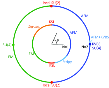
Figure 1: The ground-state phase diagram of the Z₂$\times$ SU($N$)_o Kitaev-Heisenberg model as a function of the angle $\varphi$.

III Results

For concreteness, we consider on a link $\boldsymbol{i},\boldsymbol{j}$ defining a nearest-neighbor $\delta$-bond of the honeycomb lattice, $\Gamma_{\delta}^{\alpha,\beta}=2K\delta_{\alpha,\beta}\delta_{\delta,\alpha}$ and $J_{\delta}=J$ in Eq. (14) to simulate the Kitaev-Heisenberg model at $N=2$. When $K$ is set to zero, the global symmetry inherent in this Heisenberg model is SU(4). At any finite values of $K$, this symmetry is reduced to a Z₂$\times$SU(2)_o one in which Z₂ corresponds to the invariance under the inversion $\boldsymbol{\boldsymbol{S}}_{\boldsymbol{i}}\rightarrow-\boldsymbol{\boldsymbol{S}}_{\boldsymbol{i}}$. We adopt the parametrization $K=A{\rm{sin}}(\varphi)$, $J=A{\rm{cos}}(\varphi)$, with $A=\sqrt{K^{2}+J^{2}}$. We simulated lattices with $L\times L$ unit cells (each containing two orbitals, i.e., $N_{s}=2L^{2}$ sites on the honeycomb lattice) and periodic boundary conditions. Henceforth, we use $A=1$ as the energy unit. As for the Trotter discretization we have used $\Delta\tau=0.1$ and values of $\beta U=10$ were found to be sufficient to guarantee projection to the odd parity sector. We have used a range of temperature $T\in[1/200,1/80]$ depending upon the considered parameter and this choice of temperature yields results representative of the ground state. Fig. 1 shows the ground-state phase diagram as a function of the angle $\varphi$ as obtained from a finite-size scaling analysis. To map out the phase diagram, we measure correlation functions of the spin operators $\hat{\boldsymbol{S}}_{\boldsymbol{i}}$, SU($N$)_o generators $\hat{\boldsymbol{T}}_{\boldsymbol{i}}$, and dimer operators $\hat{D}_{\boldsymbol{i},\alpha}^{T}=\hat{\boldsymbol{T}}_{\boldsymbol{i}}\cdot\hat{\boldsymbol{T}}_{\boldsymbol{i}+\boldsymbol{\delta}_{\alpha}}$ for each-$\delta_{\alpha}$ bond. The ground-state phase diagram at $N=1$ has been studied to date [26; 27] [see Fig. 1], and leads to antiferromagnetic (AFM), ferromagnetic (FM), zig-zag, and stripy ordered states, and Kitaev spin liquid (KSL) states. We find that the $N=2$ deformations of the $N=1$ Kitaev-Heisenberg model show different ground-state properties. Aside from the AFM and FM ordered states with spontaneous broken SU(2)_o symmetry and the Kekulé valence bond solid (KVBS) ordered state with a spontaneously broken translation symmetry, we observe that the KSL states are absent and that states with higher global SU(4) and local SU(2)_o continuous symmetries arise.

Figure 2: Real-space correlations of $\hat{S}^{1}$ [(a), (b)] and $\hat{\boldsymbol{T}}$ [(c), (d)] and dynamical structure factor of $\hat{\boldsymbol{T}}$ generators, $C^{T}(\boldsymbol{q},\omega)$ [(e), (f)] in the Kitaev limits at $N=2$. (a), (c), (e) $\varphi/\pi=0.5$ [AFM Kitaev limit] and (b), (d), (f) $\varphi/\pi=1.5$ [FM Kitaev limit]. (g) First (solid) and second (dashed line) Brillouin zones. Results in (e), (f) correspond to scans along the red line. Here, $L=9$ and $T=1/200$.

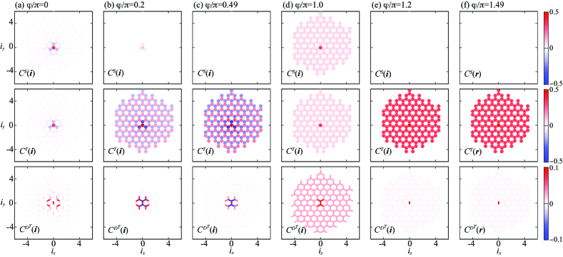
Figure 3: Real-space correlations of $\hat{S}^{1}$ (top panel), $\hat{\boldsymbol{T}}$ (middle panel), and $\hat{D}^{T}$ (bottom panel) at different values of the angle $\varphi$. (a), (b), (d), (e) $T=1/80$ and (c), (f) $T=1/200$. Here, $L=9$ and $N=2$.

III.1 Kitaev limits

We first examine the Kitaev limits (AFM case, $\varphi/\pi=0.5$, and FM case, $\varphi/\pi=1.5$), the Z₂$\times$ SU($N$)_o Kitaev model at $N=2$. In this case the Hamiltonian is given by:

$$\hat{H}=|K|\sum_{b}\hat{O}_{b}^{\dagger}\hat{O}^{\phantom{\dagger}}_{b}+U\sum_{\boldsymbol{i}}\left(\hat{n}_{\boldsymbol{i}}-N\right)^{2}$$ (21)

with $\hat{O}_{b}=\hat{S}_{\boldsymbol{i}}^{\alpha}+\frac{K}{|K|}\hat{S}_{\boldsymbol{i}+\boldsymbol{\delta}_{\alpha}}^{\alpha}$ and $\hat{n}_{\boldsymbol{i}}=\sum_{s,n}\hat{f}^{\dagger}_{\boldsymbol{i},s,n}\hat{f}^{\phantom{\dagger}}_{\boldsymbol{i},s,n}$. In the large U-limit, charge fluctuations are suppressed such that $\hat{n}_{\boldsymbol{i}}|\Psi_{0}\rangle=N|\Psi_{0}\rangle$ and

$$E_{0}=|K|\sum_{b}||\hat{O}^{\phantom{\dagger}}_{b}|\Psi_{0}\rangle||^{2}\geq 0.$$ (22)

As a consequence, any wave function that satisfies $\langle\Psi_{0}|\hat{H}|\Psi_{0}\rangle=0$ is degenerate with the ground state. We now show that the ground state degeneracy is at least $3^{N_{s}}$ where $N_{s}$ is the number of sites on the honeycomb lattice. At $N=2$ each site hosts six states that we can conveniently classify as spin-singlets and orbital-triplets

$$|1,1\rangle_{o,\boldsymbol{i}} = \hat{f}^{\dagger}_{\boldsymbol{i},\uparrow,1}\hat{f}^{\dagger}_{\boldsymbol{i},\downarrow,1}|0\rangle,$$

$$|1,-1\rangle_{o,\boldsymbol{i}} = \hat{f}^{\dagger}_{\boldsymbol{i},\uparrow,2}\hat{f}^{\dagger}_{\boldsymbol{i},\downarrow,2}|0\rangle,$$

$$|1,0\rangle_{o,\boldsymbol{i}} = \frac{1}{\sqrt{2}}(\hat{f}^{\dagger}_{\boldsymbol{i},\uparrow,1}\hat{f}^{\dagger}_{\boldsymbol{i},\downarrow,2}+\hat{f}^{\dagger}_{\boldsymbol{i},\uparrow,2}\hat{f}^{\dagger}_{\boldsymbol{i},\downarrow,1})|0\rangle$$ (23)

for which

$$\hat{S}^{\alpha}_{\boldsymbol{i}}|1,m\rangle_{o,\boldsymbol{i}} = 0,$$

$$\hat{T}^{z}_{\boldsymbol{i}}|1,m\rangle_{o,i} = m|1,m\rangle_{o,\boldsymbol{i}},$$

$$\left(\hat{\boldsymbol{T}}_{\boldsymbol{i}}\right)^{2}|1,m\rangle_{o,\boldsymbol{i}} = 1(1+1)|1,m\rangle_{o,\boldsymbol{i}}$$ (24)

as well as orbital-singlets and spin-triplets

$$|1,1\rangle_{s,\boldsymbol{i}} = \hat{f}^{\dagger}_{\boldsymbol{i},\uparrow,1}\hat{f}^{\dagger}_{\boldsymbol{i},\uparrow,2}|0\rangle,$$

$$|1,-1\rangle_{s,\boldsymbol{i}} = \hat{f}^{\dagger}_{\boldsymbol{i},\downarrow,1}\hat{f}^{\dagger}_{\boldsymbol{i},\downarrow,2}|0\rangle,$$

$$|1,0\rangle_{s,\boldsymbol{i}} = \frac{1}{\sqrt{2}}(\hat{f}^{\dagger}_{\boldsymbol{i},\uparrow,1}\hat{f}^{\dagger}_{\boldsymbol{i},\downarrow,2}+\hat{f}^{\dagger}_{\boldsymbol{i},\downarrow,1}\hat{f}^{\dagger}_{\boldsymbol{i},\uparrow,2})|0\rangle$$ (25)

for which

$$\hat{T}^{\alpha}_{\boldsymbol{i}}|1,m\rangle_{s,\boldsymbol{i}} = 0$$

$$\hat{S}^{z}_{\boldsymbol{i}}|1,m\rangle_{s,\boldsymbol{i}} = m|1,m\rangle_{s,\boldsymbol{i}},$$

$$\left(\hat{\boldsymbol{S}}_{\boldsymbol{i}}\right)^{2}|1,m\rangle_{s,\boldsymbol{i}} = 1(1+1)|1,m\rangle_{s,\boldsymbol{i}}.$$ (26)

As a consequence and for an arbitrary set of $m_{\boldsymbol{i}}\in\left\{-1,0,1\right\}$,

$$|\Psi_{0}\rangle=\otimes_{\boldsymbol{i}}|1,m_{\boldsymbol{i}}\rangle_{o,\boldsymbol{i}}$$ (27)

is a ground state. Hence the ground state manifold is at least $3^{N_{s}}$ degenerate.

We will now show that the QMC data is consistent, with the ground state being in the aforementioned manifold of states. In fact, for any $|\Psi_{0}\rangle$ given by Eq. (27) we have

$$C^{S}(\boldsymbol{i})=\langle\hat{S}_{\boldsymbol{i}}^{1}\cdot\hat{S}_{\boldsymbol{0}}^{1}\rangle=0.$$ (28)

Note that the above holds for any $\alpha$ and our numerical data confirm this point of view. Our Hamiltonian has a local orbital rotational symmetry,

$$\left[\hat{H},\hat{\boldsymbol{T}}_{\boldsymbol{i}}\right]=0$$ (29)

such that

$$C^{T}(\boldsymbol{i})=\langle\hat{\boldsymbol{T}}_{\boldsymbol{i}}\cdot\hat{\boldsymbol{T}}_{\boldsymbol{0}}\rangle=\delta_{\boldsymbol{i},\boldsymbol{0}}1(1+1).$$ (30)

In Figs. 2(a)-(d) we plot the correlators of the generators of spin and orbital rotations. As apparent, the QMC data show $C^{S}(\boldsymbol{i})=0$ as well as $C^{T}(\boldsymbol{i})=2\delta_{\boldsymbol{i},\boldsymbol{0}}$, in accord with the above.

Finally, we consider the dynamical structure factor of the $\hat{\boldsymbol{T}}$ generators. This quantity is defined as $C^{T}(\boldsymbol{q},\omega)=\text{Im}\chi(\boldsymbol{q},\omega)/\left(1-e^{-\beta\omega}\right)$ with

$$\chi(\boldsymbol{q},\omega) =\frac{i}{3}\sum_{\gamma}\int_{0}^{\infty}dt\,e^{i\omega t}\left<\left[\hat{T}^{\gamma}_{\boldsymbol{q}},\hat{T}^{\gamma}_{\boldsymbol{-q}}(-t)\right]\right>$$ (31)

where $\hat{T}^{\alpha}_{\boldsymbol{q}}=\frac{1}{\sqrt{V}}\sum_{\boldsymbol{i}}e^{i\boldsymbol{q}\cdot\boldsymbol{i}}\left(\hat{T}^{\alpha}_{\boldsymbol{i},A}+\hat{T}^{\alpha}_{\boldsymbol{i},B}e^{i\boldsymbol{q}\boldsymbol{R}}\right)$. Here $\boldsymbol{i}$ runs over the $A$ sublattice (or unit cell) on the honeycomb lattice, and $\boldsymbol{R}=2/3(\boldsymbol{a_{2}}-\boldsymbol{a_{1}}/2)$ with $\boldsymbol{a_{1}}$ and $\boldsymbol{a_{2}}$ the lattice vectors. We compute this quantity using the stochastic analytical continuation [28] as implemented in the ALF [24] library. Our QMC results at $\varphi/\pi=0.5$ and $\varphi/\pi=1.5$ are shown in Figs. 2(e) and 2(f). One observes that the spectrum has no momentum dependence and is apparently gapless at any wave vector $\boldsymbol{q}$. The absence of momentum dependence stems from the local SU(2) invariance in orbital space [see Eq. (29)]. We also observe that the spectral function does not pick up excited states. This stems from the fact that the matrix element

$${}_{s,\boldsymbol{i}}\langle 1,m|\hat{T}_{\boldsymbol{i}}^{\alpha}|1,m^{\prime}\rangle_{o,\boldsymbol{i}}$$ (32)

vanishes identically.

Figure 4: (a) Correlation ratios for AFM (upper panel) and KVBS (down panel) states at different values of $\varphi/\pi$ close to the SU(4) symmetric AFM Heisenberg point at $\varphi/\pi=0$. (b) Correlation ratio for a FM state at different values of $\varphi/\pi$ close to the SU(4) symmetric FM Heisenberg point at $\varphi/\pi=1.0$. Here, $T=1/80$.

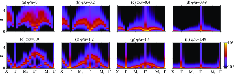
Figure 5: Dynamical structure factor of $\hat{\boldsymbol{T}}$ generators, $C^{T}(\boldsymbol{q},\omega)$ at different values of the angle $\varphi$. (a), (b), (c), (e), (f), (g) $T=1/80$ and (d), (h) $=1/200$. Results correspond to scans along the red line of first and second Brillouin zones in Fig. 2(g). Here, $L=9$ and $N=2$.

III.2 From Kitaev to Heisenberg

As argued above, in the Kitaev limits, a local SU(2) symmetry renders the ground state macroscopically degenerate: each site as a three fold degeneracy akin to a spin-1 orbital degree of freedom (see Eq. (III.1)). As soon as the local SU(2) symmetry is lifted, an S=1 orbital antiferromagnetic ($\phi/\pi=0.49$), Fig. 3(c), and S=1 orbital ferromagnetic ($\phi/\pi=1.49$) Fig. 3(f), become apparent. This state is picked up by the vanishing of the spin correlation function, $C^{S}(\boldsymbol{i})$, and ferromagnetic or anti-ferromagnetic ordering in the orbital degrees of freedom, $C^{T}(\boldsymbol{i})$. Alongside the spin and orbital correlation functions we consider dimer-dimer ones that are defined as: $C^{D^{T}}(b)=\langle(\hat{{D}}_{b}^{T}-\langle\hat{{D}}_{b}^{T}\rangle)(\hat{{D}}_{0}^{T}-\langle\hat{{D}}_{0}^{T}\rangle)\rangle$. For a given bond $b=(\boldsymbol{i},\boldsymbol{j})$, $\hat{{D}}_{b}^{T}=\boldsymbol{\hat{T}}_{\boldsymbol{i}}\cdot\boldsymbol{\hat{T}}_{\boldsymbol{j}}$. We note that the dimer-dimer correlation function is a SU(2)_o singlet as it remains invariant under SU(2)_o rotations. At the Kitaev points this quantity vanishes due to the local SU(2)_o symmetry. Away from this point it is interesting to see that it shows substantial ferromagnetic correlations. This correlation pattern does not break any further symmetries and merely reflects the ferromagnetic long-ranged correlations, Figs. 3(d)-(f).

We note that in a large region around the Kitaev points, the spin-spin correlations $C^{S}(\boldsymbol{i})$, remain very small in comparison to the orbital ones, Figs. 3(b) and 3(e). This reflects one of the key points of our model: by enhancing the symmetry from Z₂ to Z${}_{2}\times SU(2)_{o}$ one provides a means to avoid frustration via a spin-flop type transition. The spin flop transition is particularly visible in the vicinity of the SU(4) ferromagnetic point, Fig. 3(d). Here, global SU(4) rotations leave the Hamiltonian invariant, and one can find one that rotates $\hat{\boldsymbol{T}}_{\boldsymbol{i}}$ to $\hat{\boldsymbol{S}}_{\boldsymbol{i}}$. As a consequence, both $C^{S}(\boldsymbol{i})$ and $C^{T}(\boldsymbol{i})$ are, as apparent in Fig. 3(d), identical, and show substantial ferromagnetic correlations. Away from this point, at $\varphi/\pi=1.2$ in Fig. 3(d), ferromagnetism is apparent only in the orbital degrees of freedom. To quantify this spin-flop transition, we consider the correlation ratio. For a general observable $O$ with correlations,

$$C^{O}_{\gamma\delta}(\boldsymbol{q})=\frac{1}{L^{2}}\sum_{\boldsymbol{R}\boldsymbol{R}^{\prime}}C^{O}_{\boldsymbol{R}\gamma,\boldsymbol{R}^{\prime}\delta}e^{i{\boldsymbol{q}}\cdot(\boldsymbol{R}-\boldsymbol{R}^{\prime})}$$ (33)

where $\boldsymbol{R},\boldsymbol{R}^{\prime}$ labels the unit cell and $\gamma,\delta$ the orbitals, it is given by

$$R^{O}=1-\frac{\lambda_{1}^{O}({\boldsymbol{q}}_{0}+\delta{\boldsymbol{q}})}{\lambda_{1}^{O}({\boldsymbol{q}}_{0})}$$ (34)

Here, $\lambda_{1}({\boldsymbol{q}})$ is the largest eigenvalue of the $C^{O}_{\gamma\delta}(\boldsymbol{q})$ matrix and ${\boldsymbol{q}}_{0}$ is the ordering wave vector and ${\boldsymbol{q}}_{0}+\delta{\boldsymbol{q}}$ the largest wave-length fluctuation of the ordered state on a given lattice size. $R^{O}$ is a renormalization group invariant quantity [29; 30]. $R_{O}\to 1$ for $L\to\infty$ in the ordered state, whereas $R_{O}\to 0$ in the disordered state. At the critical point, $R^{O}$ is scale-invariant for sufficiently large $L$ so that results for different system sizes cross. Fig. 4(b) shows this quantity around the SU(4) ferromagnetic point. As apparent there is a singularity at the SU(4) point, that reflects the spin-flop transition. For the considered totally antisymmetric self-conjugate representation of SU(4), the ferromagnetic state has a U(2)$\times$U(2) symmetry whereas the Hamiltonian an U(4) one. This gives rise to a total of $\text{dim}\frac{U(N)}{U(N/2)\times U(N/2)}=\frac{N^{2}}{2}\equiv n_{BG}$ of flat directions of the fluctuations of the order parameter or equivalently the number of broken generators. As summarized in Ref. [31], for non-relativistic systems $n_{BG}$ does not match the number of Goldstone modes, $n_{NGM}$. In fact $n_{NGM}=n_{BG}-\frac{1}{2}\text{rank}\left(\rho\right)$ where $\rho_{\alpha,\beta}=-\frac{i}{N_{s}}\langle\Psi_{0}|\left[\hat{T}^{\alpha},\hat{T}^{\beta}\right]|\Psi_{0}\rangle$ and $|\Psi_{0}\rangle$ is the broken symmetry ground state and $\hat{T}^{\alpha}=\sum_{\boldsymbol{i}}\hat{T}_{\boldsymbol{i}}^{\alpha}$ the generators of the global SU($N$) symmetry. Hence, over the spin-flop transition, the number of Goldstone modes change abruptly from 4 ($N=4$) to 1 ($N=2$). Thereby fluctuations around the ordered state are abruptly suppressed and the ordering is more robust. Magnetically ordered states for the same representation of SU($N$) were studied in Ref. [32]. Finally we note that away from the SU(4) symmetric point, the correlation ratio is next to angle independent. This behavior is a direct consequence of the fact that the largest eigenvalue $\lambda_{1}({\boldsymbol{q}}=\boldsymbol{0})$ merely corresponds to the total spin, a quantity that is determined by symmetry and not by Hamiltonian dynamics.

We now consider the SU(4) symmetric isotropic AFM Heisenberg realized at $\varphi/\pi=0$. The ground state of this model has been reported earlier and corresponds to the KVBS ordered state [33; 34]. Our data, Fig. 3(a), supports this point of view since the dimer-dimer correlation ratio grows as a function of system size whereas the AFM one decreases. The KVBS state is a gaped state with discrete $C_{3}$ broken symmetry such that we expect this phase to be robust to perturbations. As apparent there is a small window around the SU(4) symmetric point, where the data is consistent with the stability of the KVBS phase. Beyond the SU(4) point, where the model has an Z${}_{2}\times$SU(2)_o symmetry the data supports a continuous transition between the KVBS and AFM phases. Within the theory of deconfined quantum criticality [35], such an order to order transition requires the emergence of a U(1) spin-liquid state at criticality. We will see that the dynamical orbital structure factor supports the interpretation of a two-spinon continuum akin to such a phase [36]. Note that the phase boundaries in Fig. 1 are based on the crossing points of results for $L=9,12$.

As mentioned above, we now turn our attention to the evolution of the dynamical structure factor of the $\hat{\boldsymbol{T}}$ generators, $C^{T}(\boldsymbol{q},\omega)$. Fig. 5 shows typical results at different values of the angle $\varphi$. At $\varphi/\pi=0$, Fig. 5(a), we are in the KVBS phase in the proximity of the deconfined quantum critical point. The data shows a small gap, and a continuum of excitations akin to the two-spinon continuum of a gapless U(1) spin liquid. As the angle grows spinons bind to form a spin-wave excitation, Figs. 5(b)-(d), the velocity of which decreases continuously and vanishes at the Kitaev point $\varphi/\pi=0.5$.

At $\varphi/\pi=1.0$, Fig. 5(e), the result for $C^{T}(\boldsymbol{q},\omega)$ produces a well-known quadratic low-lying dispersion around $\boldsymbol{\Gamma}$ point. Moving towards the Kitaev limits [Figs. 5(f)-(h)] the data again shows the reduction of the spin-wave velocity in the vicinity of the $\boldsymbol{\Gamma}$ or $\boldsymbol{\Gamma}^{\prime}$ points.

IV Summary

Using a phase pinning approach, we have introduced a set of Z${}_{2}\times$ SU($N$)_o generalized Kitaev models that are free of the negative sign problem for even $N$ within auxiliary field quantum Monte Carlo simulations. Our formulation is based on the Abrikosov fermion representation of the spin-1/2 algebra. The demonstration of the absence of the sign problem stems from the consequence that the imaginary part of the action is quantized to 2$\pi$ by enhancing the number of fermion orbitals from one to $2N$. This idea allows to provide a generic guideline for defining a set of sign-free models with higher symmetries. In fact, such a strategy was followed for the Hubbard model in Ref. [21] to stabilize stripes in doped quantum anti-ferromagnets.

We have used this formulation to investigate the ground-state properties of the Z${}_{2}\times$SU($2$)_o Kitaev-Heisenberg model. Generically, it is hard to predict the effect of this symmetry enhancement on the ground state phase diagram. In the specific case of the Kitaev model, it turns out that the symmetry enhancement provides a route to avoid frustration. That is, at generic angles where the symmetry is not enhanced, the spin-spin correlations vanish and ordering occurs in the orbital degrees of freedom. Although the Kitaev spin liquid phases inherent in original Z₂ symmetric model are not present the ground-state phase diagram of the symmetry enhanced model is extremely rich. Aside from the antiferromagnetic and ferromagnetic ordered states with a spontaneously broken SU(2)_o symmetry and the Kekulé valence bond solid ordered state with a spontaneously broken translation symmetry, we observe states with higher global SU(4) and local SU(2)_o continuous symmetries. The model equally supports a de-confined quantum critical point between the KVBS and AFM with emergent U(1) spin liquid state.