A note on bifurcations from eigenvalues of the Dirichlet-Laplacian with arbitrary multiplicity

Abstract

In this short note, we consider the elliptic problem

$$\lambda\phi+\Delta\phi=\eta|\phi|^{\sigma}\phi,\quad\phi\big{|}_{\partial\Omega}=0,\quad\lambda,\eta\in{\mathbb{C}},$$

on a smooth domain $\Omega\subset{\mathbb{R}}^{N}$, $N\geq 1$. The presence of complex coefficients, motivated by the study of complex Ginzburg-Landau equations, breaks down the variational structure of the equation. We study the existence of nontrivial solutions as bifurcations from the trivial solution. More precisely, we characterize the bifurcation branches starting from eigenvalues of the Dirichlet-Laplacian of arbitrary multiplicity. This allows us to discuss the nature of such bifurcations in some specific cases. We conclude with the stability analysis of these branches under the complex Ginzburg-Landau flow. Keywords: complex Ginzburg-Landau, bound-states, bifurcation. AMS Subject Classification 2010: 35Q56, 35B10, 35B32, 35B35.

1 Introduction

1.1 Description of the problem and main results

Consider the complex Ginzburg-Landau equation on a smooth domain $\Omega\subset{\mathbb{R}}^{n}$ and Dirichlet boundary conditions:

$$\begin{cases}v_{t}=e^{i\theta}\Delta v+e^{i\gamma}|v|^{\sigma}v+kv,\quad v=v(x,t),\,(x,t)\in\Omega\times[0,T]\\ v\big{|}_{\partial\Omega\times(0,T)}=0\end{cases}\mbox{for }\gamma,k\in{\mathbb{R}},\ |\theta|<\pi/2,\ \sigma>0,$$ (CGL)

The Ginzburg-Landau equation is a model for several physical and chemical phenomena such as superconductivity or chemical turbulence. We refer [15], [23] and the references cited therein. A very interesting remark is the fact that (CGL) can be viewed as a dissipative version of the nonlinear Schödinger equation, which admits solutions developing localized singularities in finite time. Local existence, global existence and uniqueness of solutions of (CGL) are widely studied on both ${\mathbb{R}}^{N}$ or a domain $\Omega\subset{\mathbb{R}}^{N}$ under various boundary conditions and assumptions on the parameters; see [16, 18, 19, 26] and the references therein. On the other hand, there are not many results concerning the blow-up of the solutions of (CGL): we refer e.g. [4] and [22].

In the analysis of evolution partial differential equations which possess a gauge invariance (see Definition 2.2), one may look for particular solutions - bound-states - of the form $e^{i\omega t}u(x)$. In the case of the the Ginzburg-Landau equation above, the profile $u$ must satisfy the stationary problem

$$i\omega u=e^{i\theta}\Delta u+e^{i\gamma}|u|^{\sigma}u+k\phi\quad\mbox{ in }\Omega,\quad u\big{|}_{\partial\Omega}=0.$$ (1)

We rewrite equation (1) in the more convenient way

$$\lambda u+\Delta u=\eta|u|^{\sigma}u,\quad\lambda,\eta\in{\mathbb{C}}.$$ (BS)

For $\lambda,\eta\in{\mathbb{R}}$, there is an extensive theory on the existence and qualitative properties of solutions to (BS). On one hand, one may take advantage of the variational structure (that is, the fact that the equation corresponds to the critical points of a well-behaved functional) to construct solutions via minmax arguments, depending on the signs of $\lambda$, $\eta$ (for $\eta<0$, one usually requires a subcritical nonlinearity, $\sigma<4/(N-2)^{+}$). The literature on variational arguments is too vast, we simply refer to the books [1], [2] and references therein. On the other hand, one may explore the existence of small solutions through the application of bifurcation arguments, starting from the eigenvalue problem $\lambda\phi+\Delta\phi=0$. For simple eigenvalues, a direct Implicit Function Theorem argument can be applied. For eigenvalues of odd multiplicity, the existence of bifurcation branches can be shown using the Leray-Schauder topological degree ([21]). For general multiple eigenvalues, one may apply a Lyapunov-Schmidt reduction and solve a nonlinear problem on the corresponding eigenspace. This approach is quite standard, see for example [3, 10, 12, 14, 25]. In the presence of symmetries (e.g. when $\Omega$ is a disk), more refined results can be found in [24] and [13]. Finally, in some very specific cases, one can characterize exactly all bifurcation branches: see [14], for the second eigenvalue in the square, and also [25], for either the case of general eigenvalues in a rectangle or the second eigenvalue in a cube.

For complex $\lambda$ and $\eta$, the known results are much more scarce. In fact, the variational structure collapses and the min-max arguments available in the real-coefficients case are of no use. Another approach is to reduce the general (BS) (via a nontrivial transformation) to the real coefficients case. This approach, available for $\Omega={\mathbb{R}}$ ([8]), seems innaplicable for any other domain. This leaves us reduced to the construction of solutions via bifurcation arguments. In the past decade, there have been some works in this direction [5, 6, 8, 9], where one applies a bifurcation argument starting from a solution to (BS) with real coefficients. Observe that, once one considers complex coefficients, all eigenvalues have even real multiplicity and one cannot apply the results of [21]. The results of [12] also do not fit our framework, as the general bifurcation results presented therein are restricted to the real-valued case.

Our main goal in this short note is to state precisely a bifurcation result for (BS) in the spirit of [10], starting from eigenvalues of any multiplicity and for $\eta\in{\mathbb{C}}$. The first result gives sufficient conditions for the existence of bifurcation branches (cf. Definition 2.1 below):

Theorem 1.1.

Fix $N\geq 1$. Let $\Omega\subset{\mathbb{R}}^{N}$ be a bounded domain and $1\leq\sigma\leq 4/(N-2)^{+}$. Let $\tilde{\lambda}$ be an eigenvalue of the Dirichlet-Laplace operator with multiplicity $p\geq 2$, with $L^{2}$-orthogonal real-valued eigenfunctions $u_{1},\dots,u_{p}$. Suppose that the system

$$\begin{split}&P_{m}(\alpha_{2},\dots,\alpha_{p})=\int_{\Omega}\left|u_{1}+\sum_{j=2}^{p}\alpha_{j}u_{j}\right|^{\sigma}\left(u_{1}+\sum_{j=2}^{p}\alpha_{j}u_{j}\right)(\alpha_{m}u_{1}-u_{m})dx=0,\quad m=2,\dots,p\end{split}$$ (2)

has a solution ${\boldsymbol{\alpha}}^{0}=(\alpha_{2}^{0},\ldots,\alpha_{p}^{0})\in{\mathbb{C}}^{p-1}\simeq{\mathbb{R}}^{2p-2}$ such that

$$\frac{\partial(P_{2},\ldots,P_{p})}{\partial(\alpha_{2},\ldots,\alpha_{p})}(\boldsymbol{\alpha}^{0})\neq 0.$$ (3)

Then there exists $\delta>0$ and a Lipschitz mapping

$$\varepsilon\in[0,\delta)\rightarrow(y,\lambda,\boldsymbol{\alpha})\in H_{0}^{1}(\Omega)\times{\mathbb{C}}\times{\mathbb{C}}^{p-1}$$

with $(y(0),\lambda(0),\boldsymbol{\alpha}(0))=(0,\tilde{\lambda},\boldsymbol{\alpha}^{0})$ and $(y,u_{i})_{L^{2}(\Omega)}=0,i=1,\ldots,p$, such that

$$(\lambda(\epsilon),u(\epsilon)):=\left(\lambda(\epsilon),y(\varepsilon)+\varepsilon u_{1}+\varepsilon\sum_{j=2}^{p}\alpha_{j}(\varepsilon)u_{j}\right)$$ (4)

is a bifurcation branch starting from $(\tilde{\lambda},0)$. Moreover, $\|y(\varepsilon)\|_{H^{1}_{0}}\leq C\varepsilon^{\sigma+1}$ and

$$\lambda(\varepsilon)=\tilde{\lambda}+\eta\varepsilon^{\sigma}\int_{\Omega}\left|u_{1}+\sum_{j=2}^{p}\alpha_{j}^{0}u_{j}\right|^{\sigma}\left(u_{1}+\sum_{j=2}^{p}\alpha_{j}^{0}u_{j}\right)u_{1}dx+o(\varepsilon^{\sigma})$$ (5)

Remark 1.2.

We observe that the conditions presented in the above theorem are completely independent on the parameter $\eta\in{\mathbb{C}}$. This is not to say that the branch is independent on $\eta$ (when $\eta$ is not real, both $\lambda$ and $u$ cannot be real, by direct integration of (BS)).

Remark 1.3.

We only guarantee that the resulting bifurcation branches are Lipschitz continuous because we will apply an Implicit Function Theorem for Lipschitz functions. This could be further improved, but we do not pursue this here. In [14] and [25], the resulting branches are $C^{1}$.

Remark 1.4.

If $\eta\in{\mathbb{R}}$ and the assumptions of Theorem 1.1 are satisfied for some $\boldsymbol{\alpha}_{0}\in{\mathbb{R}}^{p-1}$, then the corresponding bifurcation branch will be real-valued. Indeed, it suffices to go through the proof of Theorem 1.1 and replace the field ${\mathbb{C}}$ with ${\mathbb{R}}$.

Remark 1.5.

Our methodology could be applied to recover the bifurcation result for simple eigenvalues from [8] (analogous to the real-valued case [3, 5, 10]): if $\tilde{\lambda}$ is a simple eigenvalue of the Dirichlet-Laplace operator with eigenfunction $u_{1}$, there exists a unique bifurcation branch (modulo gauge symmetry) in the neighbourhood of $(\tilde{\lambda},0)$ defined by

$$\phi=y(\varepsilon)+\varepsilon u_{1}\quad{\it and}\quad\lambda(\varepsilon)=\tilde{\lambda}+\eta\varepsilon^{\sigma}\int_{\Omega}|u_{1}|^{\sigma}u_{1}^{2}dx+o(\varepsilon^{\sigma}).$$

Our second result complements Theorem 1.1, as it relates bifurcation branches to solutions of (2).

Theorem 1.6.

Fix $N\geq 1$. Let $\Omega\subset{\mathbb{R}}^{N}$ be a bounded domain and $1\leq\sigma<4/(N-2)^{+}$. Let $\tilde{\lambda}$ be an eigenvalue of the Dirichlet-Laplace operator with multiplicity $p\geq 2$, with $L^{2}$-orthogonal real-valued eigenfunctions $u_{1},\dots,u_{p}$. Suppose that $(\lambda,u):[0,\delta)\to{\mathbb{C}}\times H^{1}_{0}(\Omega)$ is a bifurcation branch starting at $(\tilde{\lambda},0)$. Given $\epsilon_{n}\to 0$, there exists $u_{0}\in H^{1}_{0}(\Omega)\setminus\{0\}$ with $-\Delta u_{0}=\tilde{\lambda}u_{0}$ such that, up to a subsequence, $u(\epsilon_{n})/\|u(\epsilon_{n})\|_{L^{\infty}}\to u_{0}$ in $H^{1}_{0}(\Omega)\cap L^{\infty}(\Omega)$. After a possible reordering of $u_{1},\dots,u_{p}$, write

$$u_{0}=c(u_{1}+\alpha_{2}u_{2}+\dots+\alpha_{p}u_{p}),\quad c,\alpha_{2},\dots,\alpha_{p}\in{\mathbb{C}},\ c\neq 0.$$

Then $\boldsymbol{\alpha}=(\alpha_{2},\dots,\alpha_{p})$ is a solution to (2).

As a consequence, if all solutions to (2) satisfy the nondegeneracy condition (3), one may characterize all bifurcation branches:

Corollary 1.7.

Under the conditions of Theorem 1.6, suppose that all solutions to (2) satisfy the nondegeneracy condition (3). Then, for all $\epsilon\in(0,\delta)$ sufficiently small, there exists a bifurcation branch $(\lambda^{\prime},u^{\prime}):[0,\delta^{\prime})\to{\mathbb{C}}\times H^{1}_{0}(\Omega)$, built through the application of Theorem 1.1, and $\epsilon^{\prime}\in(0,\delta^{\prime})$ such that $(\lambda(\epsilon),u(\epsilon))=(\lambda^{\prime}(\epsilon^{\prime}),u^{\prime}(\epsilon^{\prime}))$, modulo gauge invariance (cf. Definition 2.2).

Remark 1.8.

Our results can also be extended (in the same spirit as [9, 14]) to the more general case $\lambda u+\Delta u=\eta|u|^{\sigma}u(1+r(x,|u|))$, with $r\in C^{1}(\Omega\times{\mathbb{R}}^{+},{\mathbb{C}})$ such that

• $r(x,0)=0$ for all $x\in\Omega$;

• There exists $\sigma_{1}>0$ with $\sigma+\sigma_{1}<4/(N-2)^{+}$ such that $|r(x,y)|\lesssim 1+|y|^{\sigma_{1}}$ for all $(x,y)\in\Omega\times{\mathbb{R}}^{+}$.

For specific domains, such as the $N$-dimensional rectangular parallelepiped, the conditions of Corollary 1.7 are verified, recovering in particular the results of [14] and [25]. Notice, however, that in [14, 25], the authors obtain $C^{1}$ branches (and not just Lipschitz) and also compute the Morse index of each bifurcation branch.

Corollary 1.9.

Take $\Omega$ be an $N$-dimensional rectangular parallelepiped and $\sigma=2$ and fix an eigenvalue $\tilde{\lambda}$ with multiplicity $p$. If $p\geq 4$, suppose additionally that any linearly independent eigenfunctions associated to $\tilde{\lambda}$, $u_{1},\dots,u_{4}$, satisfy

$$\int_{\Omega}u_{1}u_{2}u_{3}u_{4}=0.$$ (6)

Then the real solutions of (2) are given by $(\alpha_{2},\dots\alpha_{p})\in\{-1,0,1\}^{p-1}$ and there exist exactly $\frac{3^{p}-1}{2}$ real bifurcation branches starting from $(\tilde{\lambda},0)$ (modulo gauge invariance).

Remark 1.10.

In [25], assumption (6) is missing. If one considers the function $J_{\lambda}$ defined therein, one finds some terms involving the product of four different eigenfunctions. However, in their proof, these terms were overlooked. While (6) could be true for $N\geq 2$ independently on $\tilde{\lambda}$, a proof of this statement is unavailable.

Remark 1.11.

Assumption (6) does not hold in general. Indeed, if $\Omega=(0,\pi)^{4}$, one may check that

$$u_{m}(x_{1},x_{2},x_{3},x_{4})=\prod_{j=1}^{4}\sin(k_{j}^{m}x_{j}),\quad(k_{1}^{m},\dots,k_{4}^{m})=\begin{cases}(1,2,3,4),\ m=1\\ (2,3,4,1),\ m=2\\ (3,4,1,2),\ m=3\\ (4,1,2,3),\ m=4,\end{cases}$$

do not satisfy (6), despite being associated to the same eigenvalue.

Remark 1.12.

In the case of the square $\Omega=(0,\pi)^{2}$, the second eigenvalue is double, with eigenfunctions

$$u_{1}(x,y)=\sin(x)\sin(2y),\quad u_{2}(x,y)=\sin(2x)\sin(y).$$

A simple computation (see the proof of Corollary 1.9) shows that

$$P_{2}(\alpha_{2})=\frac{\pi^{2}}{8}(\alpha^{2}-1)\Re\alpha_{2}-\frac{5\pi^{2}}{64}(|\alpha_{2}|^{2}-1)\alpha_{2}.$$

Apart from the real solutions $\alpha_{2}=0,\pm 1$, one can also check that $\alpha_{2}=\pm i$ is also a solution. Therefore, the corresponding bifurcation branch will be strictly complex, even if $\eta$ is real.

Remark 1.13.

For double eigenvalues, system (2) reduces to a single equation. If $\sigma$ is even and we restrict ourselves to the real case $\alpha_{2}\in{\mathbb{R}}$, $P_{2}$ becomes a polynomial on $\alpha_{2}$. Assumming that $P_{2}\nequiv 0$, the maximum number of bifurcation branches of the form (4) is $\sigma+2$.

Remark 1.14.

In the case of the disk $\Omega=\{(x,y)\in{\mathbb{R}}^{2}:x^{2}+y^{2}=1\}$, it is known (see [11] and [24, Section 2.2]) that the second eigenvalue $\lambda_{2}$ is double. In polar coordinates, the eigenspace is generated by $u_{1}=J(r)\cos(\theta)$ and $u_{2}=J(r)\sin(\theta)$, where $J$ is the Bessel function of first kind of order 1. Then

$$P_{2}(\alpha_{2})=\int_{\Omega}|u_{1}+\alpha_{2}u_{2}|^{2}(u_{1}+\alpha_{2}u_{2})(\alpha_{2}u_{1}-u_{2})dx=C\left((\alpha_{2}^{2}-|\alpha_{2}|^{2})\alpha_{2}+2i\Im\alpha_{2}\right),\quad C\neq 0.$$

If $\alpha_{2}\in{\mathbb{R}}$, $P_{2}\equiv 0$ and, in this case, our result is not applicable. This is to be expected, since it was proven in [24] that there exists a continuum of real bifurcation branches stemming from $\lambda_{2}$. For general real bifurcation results under the presence of symmetry, the reader may also consult [13].

Having built solutions to (BS), one may now consider the stability of the corresponding bound-state under the complex Ginzburg-Landau flow. Fix an eigenvalue $\tilde{\lambda}$ and a bifurcation branch $(\lambda(\epsilon),u(\epsilon))$ starting at $(\tilde{\lambda},0)$ given either by Theorem 1.1 (in the multiple case) or by Remark 1.5 (in the simple case). Set $k(\epsilon)-i\omega(\epsilon):=e^{i\theta}\lambda(\epsilon)$. Then, as already mentioned, $v=e^{i\omega(\epsilon)t}u(\epsilon)$ solves (CGL) for $k=k(\epsilon)$.

Theorem 1.15.

Let $\Omega\subset{\mathbb{R}}^{N}$ be a bounded domain and $1\leq\sigma\leq 2/(N-2)^{+}$. Suppose that $\tilde{\lambda}$ is an eigenvalue of the Dirichlet-Laplace operator and it is not the first eigenvalue. Then, for $\varepsilon$ sufficiently small, the standing wave $u$ is orbitally unstable.

Remark 1.16.

The condition $\sigma\leq 2/(N-2)^{+}$ is only required in order to guarantee the local well-posedness of (CGL) (see [20]).

We also take this opportunity to present several examples that give some insight concerning the relationship between reflection symmetries and bifurcation branches exploited in [14]. As we will see, the equivalence found in [14] between the reflection symmetries of the square and the bifurcation branches starting at the second eigenvalue is a very particular feature and does not hold in general.

Structure of the article. In Section 2, we present the proofs of the bifurcation results (Theorems 1.1, 1.6 and their corollaries). In Section 3, we prove the instability result (Theorem 1.15). We conclude with a discussion on the connection between reflection symmetries and real bifurcation branches (Section 4).

2 Bifurcation analysis

Definition 2.1.

We say that a continuous mapping $(\lambda,u);[0,\delta)\to{\mathbb{C}}\times H^{1}_{0}(\Omega)$ is a bifurcation branch starting from $(\tilde{\lambda},0)$ if $(\lambda(0),u(0))=(\tilde{\lambda},0)$ and, for each $\epsilon\in(0,\delta)$, $u(\epsilon)$ is a nontrivial solution to (BS) with $\lambda=\lambda(\epsilon)$.

Definition 2.2.

Equation (BS) is gauge invariant: if $u$ is a solution, so is $zu$, for any $z\in\mathbb{S}^{1}:=\{z\in{\mathbb{C}}:|z|=1\}$. If $(\lambda_{1},u_{1})$ and $(\lambda_{2},u_{2})$ are two bifurcation branches defined on $[0,\delta)$ and, for each $\epsilon\in[0,\delta)$, there exists $z(\epsilon)\in\mathbb{S}^{1}$ such that $u_{1}(\epsilon)=z(\epsilon)u_{2}(\epsilon)$, we say that the branches are the same modulo gauge invariance.

Define $L=-\Delta$ and $Mu=-\eta|u|^{\sigma}u$ and

$$(u,v)_{L^{2}}=\int_{\Omega}u\overline{v}dx.$$

Represent by $V$ the corresponding eigenspace, spanned by $u_{1},\ldots,u_{p}$. Taking $P:L^{2}(\Omega)\rightarrow V^{\perp}$ and applying the Lyapunov-Schmidt reduction, equation (BS) is equivalent to the system

$$P(\lambda u-Lu+Mu) =0$$ (7)

$$(\lambda u-Lu+Mu,u_{j})_{L^{2}} =0,\,\,j=1,\ldots,p$$ (8)

We look for solutions of this system in the form

$$u=y+\sum_{j=1}^{p}\epsilon_{j}u_{j},\quad y\in V^{\perp}$$

where, without loss of generality, we may assume $\epsilon_{1}>0$ (due to the gauge invariance of the problem). From (7),

$$y=(\lambda-PL)^{-1}\Big{[}-PM(y+\sum_{j=1}^{p}\epsilon_{j}u_{j})\Big{]}$$ (9)

and

$$\epsilon_{m}(\lambda-e^{i\theta}\tilde{\lambda})=-\Big{(}M(y+\sum_{j=1}^{p}\epsilon_{j}u_{j}),u_{m}\Big{)}_{L^{2}},\quad m=1,\ldots,p.$$ (10)

Following exactly the same proof as in [9, Lemma 3.1],

Lemma 2.3.

There exists $\delta_{0}>0$ such that, for all $0<\delta<\delta_{0}$, given $\epsilon_{1},\dots,\epsilon_{p},\lambda\in{\mathbb{C}}$ with

$$|\epsilon_{j}|<\delta,\ j=1,\dots,p,\quad|\lambda-\tilde{\lambda}|<\delta,$$ (11)

there exists a unique solution $y=y(\epsilon_{1},\dots,\epsilon_{p},\lambda)\in H^{1}_{0}(\Omega)$ of (9). Moreover, for some universal constants $C>0,K>0$,

$$\|y(\epsilon_{1},\dots,\epsilon_{p},\lambda)\|_{H^{1}_{0}}\leq C\delta^{{\sigma}+1}\\$$ (12)

and

$$\|y(\epsilon_{1},\dots,\epsilon_{p},\lambda)-y(\epsilon_{1}^{\prime},\dots,\epsilon_{p}^{\prime},\lambda^{\prime})\|_{H^{1}_{0}}\leq K\delta^{{\sigma+1}}|(\epsilon_{1},\dots,\epsilon_{p},\lambda)-(\epsilon_{1}^{\prime},\dots,\epsilon_{p}^{\prime},\lambda^{\prime})|\\$$ (13)

whenever $(\epsilon_{1},\dots,\epsilon_{p},\lambda)$ and $(\epsilon_{1}^{\prime},\dots,\epsilon_{p}^{\prime},\lambda^{\prime})$ satisfy (11).

Setting $\alpha_{j}=\epsilon_{j}/\epsilon_{1}$ and taking $m=1$ in (10),

$$\begin{split}\lambda-e^{i\theta}\tilde{\lambda}&=-\frac{1}{\epsilon_{1}}\Big{(}M(y+\sum_{j=1}^{p}\epsilon_{j}u_{j}),u_{1}\Big{)}_{L^{2}}\\ &=-\epsilon_{1}^{\sigma}\Big{(}M(u_{1}+\sum_{j=2}^{p}\alpha_{j}u_{j}),u_{1}\Big{)}_{L^{2}}+Q_{1}(y,\epsilon_{1},\alpha_{2},\ldots,\alpha_{p})\\ \end{split}$$ (14)

with

$$Q_{1}(y,\epsilon_{1},\boldsymbol{\alpha})=-\frac{1}{\epsilon_{1}}\Big{(}M(y+\sum_{j=1}^{p}\epsilon_{j}u_{j})-M(\sum_{j=1}^{p}\epsilon_{j}u_{j}),u_{1}\Big{)}_{L^{2}}.$$ (15)

On the other hand, (10) also implies

$$\begin{split}\alpha_{m}\Big{(}M(y+\sum_{j=1}^{p}\epsilon_{j}u_{j}),u_{1}\Big{)}_{L^{2}}&=-\alpha_{m}\epsilon_{1}(\lambda-e^{i\theta}\tilde{\lambda})=-\epsilon_{m}(\lambda-e^{i\theta}\tilde{\lambda})\\ &=\Big{(}M(y+\sum_{j=1}^{p}\epsilon_{j}u_{j}),u_{m}\Big{)}_{L^{2}}.\\ \end{split}$$ (16)

Setting

$$Q_{m}(y,\epsilon_{1},\boldsymbol{\alpha})=\frac{1}{\epsilon_{1}^{\sigma+1}}\Big{(}M(y+\sum_{j=1}^{p}\epsilon_{j}u_{j})-M(\sum_{j=1}^{p}\epsilon_{j}u_{j}),\overline{\alpha_{m}}u_{1}-u_{m}\Big{)}_{L^{2}},$$ (17)

it follows from (16) that

$$\Big{(}M(u_{1}+\sum_{j=2}^{p}\alpha_{j}u_{j}),\overline{\alpha_{m}}u_{1}-u_{m}\Big{)}_{L^{2}}+Q_{m}=0,\,\,m=2,\ldots,p.$$ (18)

Proof of Theorem 1.1.

From the above discussion and Lemma 2.3, it suffices to prove that, setting $y=y(\epsilon_{1},\dots,\epsilon_{p},\lambda)$ given by Lemma 2.3, equations (14) and (18) define $\lambda$ and $\alpha_{j}$ implicitly as function of $\epsilon_{1}$. First, observe that, if one drops the remainder terms $Q_{m}$, the system reduces to

$$\begin{split}F_{1}(\epsilon_{1},\lambda,\alpha_{2},\ldots,\alpha_{p})&=\lambda-\tilde{\lambda}+\epsilon_{1}^{\sigma}\Big{(}M(u_{1}+\sum_{j=2}^{p}\alpha_{j}u_{j}),u_{1}\Big{)}_{L^{2}}=0\\ F_{m}(\epsilon_{1},\lambda,\alpha_{2},\ldots,\alpha_{p})&=P_{m}(\alpha_{2},\ldots,\alpha_{p})=0,\,\,m=2,\ldots,p.\end{split}$$ (19)

This system satisfies the conditions of the Implicit Function Theorem at $(\epsilon_{1},\lambda,\boldsymbol{\alpha})=(0,\tilde{\lambda},\boldsymbol{\alpha}^{0})$, since

$$\frac{\partial(F_{1},\ldots,F_{p})}{\partial(\lambda,\alpha_{2},\ldots,\alpha_{p})}(\tilde{\lambda}\leavevmode\nobreak\ ,\boldsymbol{\alpha}^{0})=\frac{\partial(P_{2},\ldots,P_{p})}{\partial(\alpha_{2},\ldots,\alpha_{p})}(\boldsymbol{\alpha}^{0})\neq 0.$$

Using the estimates (12) and (13), one may prove that $Q_{m}$, $m=1,\dots,p$ are Lipschitz continuous in $\epsilon_{1},\lambda$ and $\alpha_{m},m=2,\dots,p$, with an arbitrarily small constant (see [9, Proof of Theorem 1.4]). Therefore the system {(14),(18)} is a small Lipschitz perturbation of (19) and one may apply the Implicit Function Theorem for Lipschitz functions ([7, Section 7.1]) to finish the proof. ∎

Proof of Theorem 1.6.

The proof follows closely the argument of [14, Lemma 2.1]. Take $\epsilon_{n}\to 0$ and write $\lambda_{n}=\lambda(\epsilon_{n})$, $u_{n}=u(\epsilon_{n})$, so that $\lambda_{n}\rightarrow\tilde{\lambda}$ and $u_{n}\rightarrow 0$ in $C(\overline{\Omega})$. After normalization $\tilde{u}_{n}=u_{n}/\|u_{n}\|_{\infty}$, we obtain

$$\begin{cases}\lambda_{n}\tilde{u}_{n}+\Delta\tilde{u}_{n}+|u_{n}|^{\sigma}\tilde{u}_{n}=0\\ \tilde{u}_{n}=0\quad{\rm on}\quad\partial\Omega\end{cases}$$ (20)

Since $\tilde{u}_{n}$ is bounded in $C(\overline{\Omega})$, by compactness, $\tilde{u}_{n}\rightarrow u_{0}$ in $C(\overline{\Omega})$ and $\tilde{\lambda}u_{0}+\Delta u_{0}=0$. Moreover, since $\|\tilde{u}_{n}\|_{L^{\infty}(\Omega)}=1,$ $u\nequiv 0$. This implies that, up to reordering of $u_{1},\dots,u_{p}$,

$$u_{0}=c(u_{1}+\alpha_{2}u_{2}+\dots+\alpha_{p}u_{p})=:cu_{\boldsymbol{\alpha}},\quad c,\alpha_{2},\dots,\alpha_{m}\in{\mathbb{C}}.$$

Decomposing $\tilde{u}_{n}=\chi_{n}+\psi_{n}$ with $\chi_{n}\in V,\psi_{n}\in V^{\perp}$,

$$\tilde{\lambda}\psi_{n}+\Delta\psi_{n}+(\lambda_{n}-\tilde{\lambda})(\chi_{n}+\psi_{n})+\|u_{n}\|_{\infty}^{\sigma}|\chi_{n}+\psi_{n}|^{\sigma}(\chi_{n}+\psi_{n})=0.$$ (21)

Multiplying by $\bar{u}_{\boldsymbol{\alpha}}$ and integrating,

$$\frac{\lambda_{n}-\tilde{\lambda}}{\|u_{n}\|_{\infty}^{\sigma}}\int_{\Omega}\chi_{n}\bar{u}_{\boldsymbol{\alpha}}dx+\int_{\Omega}|\chi_{n}+\psi_{n}|^{\sigma}(\chi_{n}+\psi_{n})\bar{u}_{\boldsymbol{\alpha}}dx=0$$

Therefore

$$\lim_{n\rightarrow\infty}\frac{\lambda_{n}-\tilde{\lambda}}{\|u_{n}\|_{\infty}^{\sigma}}=-c^{\sigma}\frac{\int_{\Omega}|u_{\boldsymbol{\alpha}}|^{\sigma+2}dx}{\int_{\Omega}|u_{\boldsymbol{\alpha}}|^{2}dx}$$ (22)

Consider the elements

$$v_{\alpha_{m}}:=(\overline{\alpha_{m}}u_{1}-u_{m}),\quad m=2,\ldots,p$$

and remark that $(u_{\boldsymbol{\alpha}},v_{\alpha_{m}})_{L^{2}}=0,\,\,m=2,\ldots,p$. We multiply (21) by $\bar{v}_{\alpha_{m}}$, divide by $\|u_{n}\|_{L^{\infty}}^{\sigma}$, integrate over $\Omega$ to find

$$\frac{\lambda_{n}-\tilde{\lambda}}{\|u_{n}\|_{\infty}^{\sigma}}\int_{\Omega}\psi_{n}\overline{v_{\alpha_{m}}}+\int_{\Omega}|\tilde{u}_{n}|^{\sigma}\tilde{u}_{n}\overline{v_{\alpha_{m}}}=0$$

In the limit, we find

$$P_{m}(\alpha_{2},\dots,\alpha_{m})=\int_{\Omega}|u_{\boldsymbol{\alpha}}|^{\sigma}u_{\boldsymbol{\alpha}}(\alpha_{m}u_{1}-u_{m})=0,\quad m=2,\ldots,p$$ (23)

and $\boldsymbol{\alpha}=(\alpha_{2},\ldots,\alpha_{p})$ is a solution to (2).

∎

Proof of Corollary 1.7.

Step 1. As in the previous proof, if $\epsilon_{n}\to 0$, up to a subsequence,

$$u(\epsilon_{n})=c_{n}\|u(\epsilon_{n})\|_{\infty}(u_{1}+\alpha_{2,n}u_{2}+\dots+\alpha_{p,n}u_{p})+y_{n},\quad y_{n}\in V^{\perp},\ c_{n}\to c\neq 0,$$

and

$$(\alpha_{2,n},\dots,\alpha_{p,n})\to\boldsymbol{\alpha}\mbox{ solution to \eqref{polinomios}}.$$

Using the gauge invariance, we may assume that $c_{n}\in{\mathbb{R}}^{+}$. Since $\|u(\epsilon_{n})\|_{\infty}\to 0$ and $\lambda(\epsilon_{n})\to\tilde{\lambda}$, Lemma 2.3 implies that, for $n$ large enough, $y_{n}$ is uniquely determined by the values of

$$c_{n}\|u(\epsilon_{n})\|_{\infty},\ \alpha_{2,n},\dots,\alpha_{p,n}\ \mbox{and }\lambda(\epsilon_{n}).$$

On the other hand, the proof of Theorem 1.1 implies that $c_{n}\|u(\epsilon_{n})\|_{\infty}$ also determines uniquely the values of $\alpha_{2,n},\dots,\alpha_{p,n}$ and $\lambda(\epsilon_{n})$ in a neighbourhood of $(0,\tilde{\lambda},\boldsymbol{\alpha})$. Therefore, denoting by $(\lambda^{\prime},u^{\prime})$ by bifurcation branch built in Theorem 1.1 starting from $\boldsymbol{\alpha}$,

$$(\lambda(\epsilon_{n}),u(\epsilon_{n}))=(\lambda^{\prime}(c_{n}\|u_{n}\|_{\infty}),u^{\prime}(c_{n}\|u_{n}\|_{\infty})).$$

Step 2. Suppose that there exists a sequence $\epsilon_{n}\to 0$ for which the claimed result does not hold. By Step 1, there is a subsequence which does satisfy Corollary 1.7, leading to a contradiction. ∎

Proof of Corollary 1.9.

To reduce system (2), one computes explicitly the coefficients (as it was done in [25]). Write $\Omega=\prod_{j=1}^{N}(0,L_{j})$ and define $\phi_{k,L}(x)=\sin(k\pi x/L)$, $k\in{\mathbb{N}}$, $L>0$. Then

$$\int_{0}^{L}\phi_{k,L}(x)^{4}dx=\frac{3L}{8},\quad\int_{0}^{L}\phi_{k,L}(x)^{2}\phi_{j,L}(x)^{2}dx=\frac{L}{4},\ j\neq k.$$

The eigenspace associated to $\tilde{\lambda}$ is generated by $u_{1},\dots,u_{p}$ of the form

$$\prod_{j=1}^{N}\phi_{k_{j},L_{j}}(x_{j}),\quad\mbox{ where }(k_{1},\dots,k_{N})\in{\mathbb{N}}^{N}\mbox{ satisfies}\sum_{j=1}^{N}\frac{\pi^{2}k_{j}^{2}}{L_{j}^{2}}=\tilde{\lambda}.$$

Then, for $1\leq m\leq p$,

$$\int_{\Omega}u_{m}^{4}(x)dx=\prod_{j=1}^{N}\frac{3L_{j}}{8}=:A,\quad\int_{\Omega}u_{m}^{2}u_{k}^{2}(x)dx=\prod_{j=1}^{N}\frac{L_{j}}{4}=:B,\ k\neq m.$$

Following [25, Proof of Theorem 1.1],

$$\int_{\Omega}u_{m}^{2}(x)u_{k}(x)u_{l}(x)dx=0,\quad k\neq l.$$

Finally, by (6), if $p\geq 4$ and $k,m,l,h$ are four different indices,

$$\int_{\Omega}u_{m}(x)u_{k}(x)u_{l}(x)u_{h}(x)dx=0.$$

This allows us to compute

$$P_{m}(\alpha_{2},\dots,\alpha_{p}) =\int_{\Omega}\left|u_{1}+\sum_{j=2}^{p}\alpha_{j}u_{j}\right|^{2}\left(u_{1}+\sum_{j=2}^{p}\alpha_{j}u_{j}\right){(\alpha_{m}u_{1}-u_{m})}dx$$

$$=(B-A)(|\alpha_{m}^{2}|-1)\alpha_{m}-2B(\alpha_{m}^{2}-1)\Re\alpha_{m}.$$

Hence the real solutions to (2) are given by

$$\alpha_{m}\in\{0,\pm 1\},\quad m=2,\dots,p.$$

A simple computation shows these solutions are nondegenerate. Thus the number of bifurcations with a nonzero $u_{1}$-coefficient is $3^{p-1}$.

Next, if one looks for the branches where the $u_{1}$-coefficient is zero and the $u_{2}$-coefficient is non-zero, the same computations yield $3^{p-2}$ bifurcation branches. Iterating this procedure, the total number of bifurcations is

$$3^{p-1}+3^{p-2}+\dots+1=\frac{3^{p}-1}{2}.$$

∎

Remark 2.4.

Fix $\Omega=(0,1)^{2}$. A consequence of Corollary 1.9 is that, for cubic nonlinearities and under (6), the real bifurcation branches correspond to $(\alpha_{2}^{0},\alpha_{3}^{0})\in\{-1,0,1\}^{2}$. One may ask if the same happens for other nonlinearities. In the case of the quintic nonlinearity $\sigma=4$, the first triple eigenvalue has eigenspace generated by

$$u_{1}(x,y)=\sin(\pi x)\sin(7\pi y),\quad u_{2}(x,y)=u_{1}(y,x),\quad u_{3}(x,y)=\sin(5\pi x)\sin(5\pi y).$$

There are nine bifurcations of the form

$$u_{3}+\alpha_{2}u_{1}+\alpha_{3}u_{2}$$

for $(\alpha_{2},\alpha_{3})$ as shown in Figure 1. It becomes clear that the set of solutions to (2) becomes nontrivial for higher order nonlinearities.

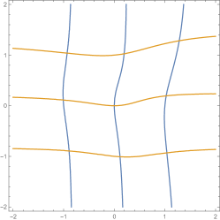
Figure 1: The nodal sets for $P_{2}$ and $P_{3}$. The nine bifurcations for which the $u_{3}$-component is nontrivial correspond to the nine intersection points.

3 Stability of bound-states under the (CGL) flow

To prove Theorem 1.15, we perform an analysis on the spectrum of the period map for the linearized equation

$$v_{t}=e^{i\theta}\Delta v+kv+B(t)v$$ (24)

with

$$B(t)v=e^{i\gamma}\left(\frac{\sigma+2}{2}|u(t)|^{\sigma}v+\frac{\sigma}{2}u(t)^{1+\sigma/2}{\bar{u}(t)}^{\sigma/2-1}\bar{v}\right)$$ (25)

Define the evolution operator $R(t,s)$ for the equation (24) as

$$R(t,s)v_{0}=v(t;s,v_{0}),$$

where $v$ is the solution of (24) with initial data $v(s)=v_{0}$. We now define the period map as the linear operator $U_{0}=R(T,0),\,T=2\pi/\omega$.

Proof of the Theorem 1.15.

Throughout the proof, it is convenient consider real spaces composed of complex valued functions. We represent them using bold face characters.

Represent by $S(t)=e^{At}$ the semigroup generated by the operator $A:=A(\varepsilon)=e^{i\theta}\Delta+k\,$, $k=\Re e^{i\theta}\lambda(\varepsilon)$. It is well-known that $S(t)$ is an analytic semigroup in ${\bf L}^{2}(\Omega)$ (see, e.g., [27, Theorem 2.7, pg. 211]). Since $\|u\|_{{\bf H}^{1}_{0}(\Omega)}=O(\epsilon)$, a standard bootstrap argument yields $\|u\|_{{\bf L}^{\infty}(\Omega)}\lesssim O(\epsilon)$. Thus the linear operator $B(t)$ referred in (25) satisfies

$$\|B(t)\|_{\mathcal{L}(\bf{L}^{2}(\Omega))} \leq\left\|\frac{\sigma+2}{2}|u(t)|^{\sigma}+\frac{\sigma}{2}u(t)^{1+\sigma/2}{\bar{u}(t)}^{\sigma/2-1}\right\|_{\bf{L}^{\infty}(\Omega)}$$ (26)

$$\leq(\sigma+1)\|u\|_{\bf{L}^{\infty}(\Omega)}^{\sigma}\leq(\sigma+1)C\varepsilon^{\sigma}$$ (27)

for all $t\in[0,T]$ and for some universal constant $C$. Consider now the linear evolution equation

$$v_{t}=Av+B(t)v.$$

Given an initial data $v_{0}\in{\bf L}^{2}(\Omega)$,

$$R(t,0)v_{0}=v(t)=S(t)v_{0}+\int_{0}^{t}S(t-s)B(s)v(s)ds$$ (28)

and

$$\|v(t)\|_{{\bf L}^{2}(\Omega)}\leq C\|v_{0}\|_{{\bf L}^{2}(\Omega)}+\int_{0}^{t}C(\sigma+1)\varepsilon^{\sigma}\|v(s)\|_{{\bf L}^{2}(\Omega)}ds$$ (29)

for all $t\in[0,T]$. Using Gronwall’s inequality, we conclude that

$$\|v(t)\|_{{\bf L}^{2}(\Omega)}\leq Ce^{CT}\|v_{0}\|_{{\bf L}^{2}(\Omega)},\quad t\in[0,T].$$ (30)

It follows from (26), (28) and (29)

$$U_{0}=S(T)+K(\varepsilon)$$ (31)

with

$$K(\varepsilon)=\int_{0}^{T}S(t-s)B(s)v(s)ds,\quad\|K(\varepsilon)\|_{\mathcal{L}({\bf L}^{2}(\Omega))}\leq C\varepsilon^{\sigma}$$ (32)

On the other hand, the spectrum of the operator $A$, $\Sigma(A)$, verifies

$$\Re\,\Sigma(A):=\{\Re\lambda:\lambda\in\Sigma(A)\}=\left\{-\cos\theta(\lambda_{j}-\tilde{\lambda})+O(\varepsilon^{\sigma})\right\}_{j\geq 1}$$ (33)

where $\lambda_{1}<\lambda_{2}\leq\lambda_{3}\leq\dots$ are the eigenvalues of the Dirichlet-Laplace operator. Since $S(t)$ is an analytic semigroup, the spectral mapping theorem establishes $\Sigma(S(T))=e^{T\Sigma(A)}$ ([17], pag. 281). Thus

$$\{|\lambda|:\lambda\in\Sigma(S(T))\}=\{e^{-T\cos\theta(\lambda_{j}-\tilde{\lambda})+O(\varepsilon^{\sigma})}\}_{j\geq 1}.$$

From (31) and (32), the period map $U_{0}$ is a small perturbation of $S(T)$, which implies the existence of an eigenvalue $\mu\in\sigma(U_{0})$ with $|\mu|>1$. Since we are working on a real Banach space and $S(t)$ is an analytic semigroup, the result now follows from [20, Th. 8.2.4].

∎

4 Real bifurcations and reflection symmetries

To conclude, we now discuss the connection between reflection symmetries of $\Omega$ and real bifurcation branches. A reflection symmetry is any reflection mapping with respect to a hyperplane which leaves $\Omega$ invariant. In particular, the hyperplane (or symmetry axis) splits $\Omega$ into two congruent domains $\Omega_{1}$ and $\Omega_{2}$ which are reflections of one another. For a given eigenvalue $\lambda$, suppose that there exists an eigenfunction which vanishes along the symmetry axis and is positive in $\Omega_{1}$. This implies in particular that $\lambda$ is the first eigenvalue in $\Omega_{1}$ and so, being simple, there exists a unique bifurcation branch when the problem is restricted to $\Omega_{1}$. Through an odd extension of the bifurcation branch to the whole $\Omega$, we then obtain a bifurcation branch for our initial problem.

In the case of the second eigenvalue of the square, the corresponding (two-dimensional) eigenspace includes four elements whose nodal lines are precisely the four reflection axii of the square:

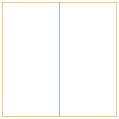
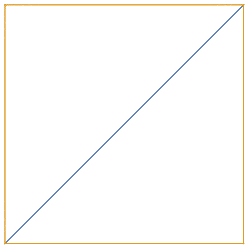
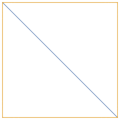
Figure 2: Nodal lines of four eigenfunctions coincide with the four reflection symmetry axii.

From Corollary 1.9, the number of bifurcation branches is $\frac{3^{2}-1}{2}=4$. Thus we conclude that all bifurcation branches arise from symmetries, as observed in [14]. This equivalence between bifurcations and symmetries does not hold in general, as one can see in the following examples concerning the bifurcation problem for $\sigma=2$:

1. (Higher dimension) For the second eigenvalue of the cube, Corollary 1.9 implies the existence of exactly thirteen bifurcation branches, which one may separate into three groups, depending on whether $\alpha_{2}^{0}$ and $\alpha_{3}^{0}$ are zero or not. The nodal sets are plotted in Figure 3. It is clear that the last four branches do not arise from any kind of reflection symmetry.

   

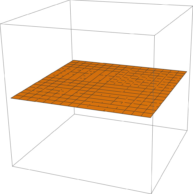
   (a) Two $\alpha$’s equal to 0 - 3 branches

   

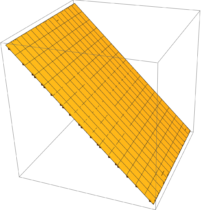
   (b) One $\alpha$ equal to 0 - 6 branches

   

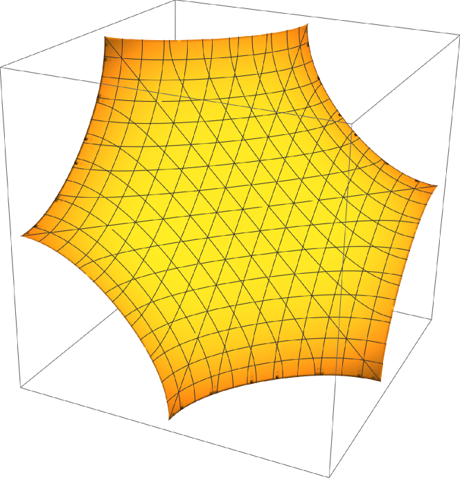
   (c) Both $\alpha$’s nonzero - 4 branches

   Figure 3: The three different types of bifurcations for the second eigenvalue in the cube.

2. (Higher eigenvalue) In the square $(0,1)^{2}$, the second multiple eigenvalue is the third one, with eigenspace generated by

   $$u_{1}(x,y)=\sin(\pi x)\sin(3\pi y),\quad u_{2}(x,y)=\sin(3\pi x)\sin(\pi y),$$

   The corresponding nodal lines are two straight vertical (or horizontal) lines, dividing the square into three congruent rectangles. The symmetry argument still applies here: one bifurcates on a single rectangle and then performs an odd extension to the whole square. However, this only accounts for two branches. For $u_{1}-u_{2}$, one sees the nodal lines are the two diagonal lines and thus the symmetry argument can still be applied (first bifurcate on one triangle and then extend to the square). The remaining branch corresponds to $u_{1}+u_{2}$, whose nodal line is represented in Figure 3.

   

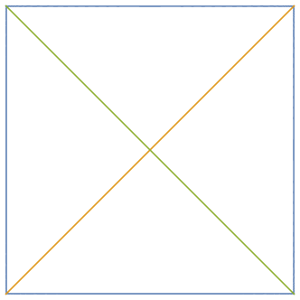
   (a) Nodal lines of $u_{1}-u_{2}$.

   

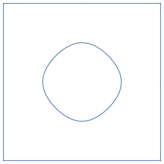
   (b) Nodal lines of $u_{1}+u_{2}$.

   Figure 4: Bifurcations from the third eigenvalue of the square.

   
   

3. (Another two-dimensional domain) In the rectangle $[0,1]\times[0,\sqrt{3/5}]$, the first double eigenvalue is the third one. The eigenspace is generated by

   $$u_{1}(x,y)=\sin(3\pi x)\sin(\sqrt{5}y/3),\quad u_{2}(x,y)=\sin(2\pi x)\sin(2\sqrt{5}y/3)$$

   The four bifurcation branches correspond to the four eigenvectors $u_{1},u_{2}$ and $u_{1}\pm u_{2}$, whose contour plot can be found in Figure 5.

   

   

   

   

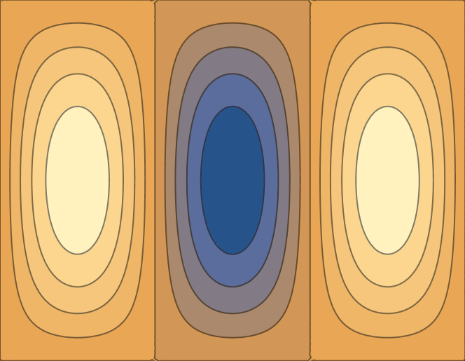
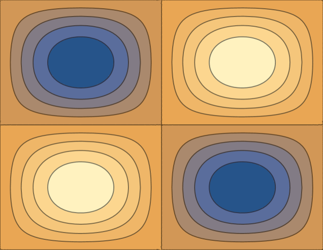
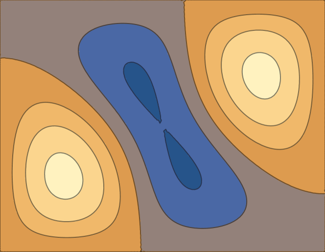
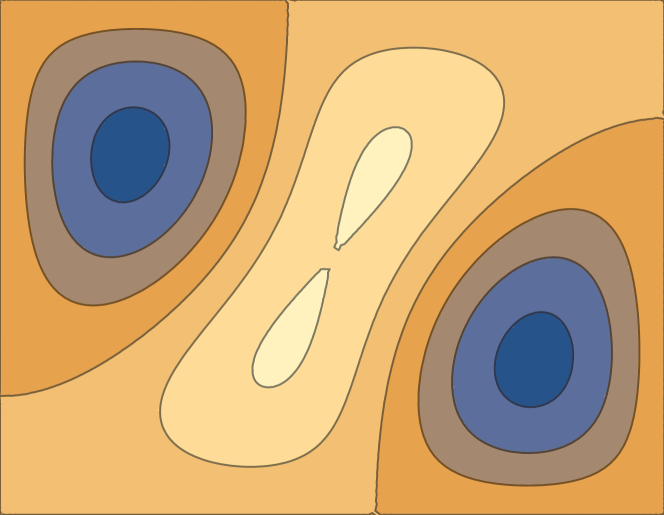
   Figure 5: Contour plot of $u_{1},u_{2}$ (top) and $u_{1}\pm u_{2}$ (bottom). The symmetry argument can only be applied to the first two cases.

Acknowledgements. The authors are indebted to Hugo Tavares, for many fruitful discussions in this topic, and also to the anonymous referee, whose comments led to a substantial improvement of the manuscript. S.C was partially supported by Fundação para a Ciência e Tecnologia, through the grant UID/MAT/04459/2019 and the project NoDES (PTDC/MAT-PUR/1788/2020). M.F. was partially supported by Fundação para a Ciência e Tecnologia, through the grant UIDB/04561/2020.

References

- [1] Antonio Ambrosetti and David Arcoya. An introduction to nonlinear functional analysis and elliptic problems, volume 82 of Progress in Nonlinear Differential Equations and their Applications. Birkhäuser Boston, Ltd., Boston, MA, 2011.
- [2] Antonio Ambrosetti and Andrea Malchiodi. Nonlinear analysis and semilinear elliptic problems, volume 104 of Cambridge Studies in Advanced Mathematics. Cambridge University Press, Cambridge, 2007.
- [3] Antonio Ambrosetti and Giovanni Prodi. A primer of nonlinear analysis, volume 34 of Cambridge Studies in Advanced Mathematics. Cambridge University Press, Cambridge, 1993.
- [4] Thierry Cazenave, Flávio Dickstein, and Fred B. Weissler. Finite-time blowup for a complex Ginzburg-Landau equation. SIAM J. Math. Anal., 45(1):244–266, 2013.
- [5] Thierry Cazenave, Flávio Dickstein, and Fred B. Weissler. Standing waves of the complex Ginzburg-Landau equation. Nonlinear Anal., 103:26–32, 2014.
- [6] Rolci Cipolatti, Flávio Dickstein, and Jean-Pierre Puel. Existence of standing waves for the complex Ginzburg-Landau equation. J. Math. Anal. Appl., 422(1):579–593, 2015.
- [7] F. H. Clarke. Optimization and nonsmooth analysis, volume 5 of Classics in Applied Mathematics. Society for Industrial and Applied Mathematics (SIAM), Philadelphia, PA, second edition, 1990.
- [8] Simão Correia and Mário Figueira. Some stability results for the complex Ginzburg-Landau equation. Commun. Contemp. Math., 22(8):1950038, 16, 2020.
- [9] Simão Correia and Mário Figueira. A generalized complex Ginzburg-Landau equation: global existence and stability results. Commun. Pure Appl. Anal., 20(5):2021–2038, 2021.
- [10] Michael G. Crandall and Paul H. Rabinowitz. Bifurcation from simple eigenvalues. J. Functional Analysis, 8:321–340, 1971.
- [11] Lucio Damascelli. On the nodal set of the second eigenfunction of the Laplacian in symmetric domains in . Atti Accad. Naz. Lincei Cl. Sci. Fis. Mat. Natur. Rend. Lincei (9) Mat. Appl., 11(3):175–181 (2001), 2000.
- [12] E. N. Dancer. Bifurcation theory in real Banach space. Proc. London Math. Soc. (3), 23:699–734, 1971.
- [13] E. N. Dancer. On the existence of bifurcating solutions in the presence of symmetries. Proc. Roy. Soc. Edinburgh Sect. A, 85(3-4):321–336, 1980.
- [14] Manuel del Pino, Jorge García-Melián, and Monica Musso. Local bifurcation from the second eigenvalue of the Laplacian in a square. Proc. Amer. Math. Soc., 131(11):3499–3505, 2003.
- [15] Charles R. Doering, John D. Gibbon, Darryl D. Holm, and Basil Nicolaenko. Low-dimensional behaviour in the complex Ginzburg-Landau equation. Nonlinearity, 1(2):279–309, 1988.
- [16] Charles R. Doering, John D. Gibbon, and C. David Levermore. Weak and strong solutions of the complex Ginzburg-Landau equation. Phys. D, 71(3):285–318, 1994.
- [17] Klaus-Jochen Engel and Rainer Nagel. One-parameter semigroups for linear evolution equations, volume 194 of Graduate Texts in Mathematics. Springer-Verlag, New York, 2000.
- [18] J. Ginibre and G. Velo. The Cauchy problem in local spaces for the complex Ginzburg-Landau equation. I. Compactness methods. Phys. D, 95(3-4):191–228, 1996.
- [19] J. Ginibre and G. Velo. The Cauchy problem in local spaces for the complex Ginzburg-Landau equation. II. Contraction methods. Comm. Math. Phys., 187(1):45–79, 1997.
- [20] Daniel Henry. Geometric theory of semilinear parabolic equations, volume 840 of Lecture Notes in Mathematics. Springer-Verlag, Berlin-New York, 1981.
- [21] M. A. Krasnosel’skii. Topological methods in the theory of nonlinear integral equations. A Pergamon Press Book. The Macmillan Company, New York, 1964. Translated by A. H. Armstrong; translation edited by J. Burlak.
- [22] Nader Masmoudi and Hatem Zaag. Blow-up profile for the complex Ginzburg-Landau equation. J. Funct. Anal., 255(7):1613–1666, 2008.
- [23] Alexander Mielke. The Ginzburg-Landau equation in its role as a modulation equation. In Handbook of dynamical systems, Vol. 2, pages 759–834. North-Holland, Amsterdam, 2002.
- [24] Yasuhito Miyamoto. Global branches of sign-changing solutions to a semilinear Dirichlet problem in a disk. Adv. Differential Equations, 16(7-8):747–773, 2011.
- [25] Dimitri Mugnai and Angela Pistoia. On the exact number of bifurcation branches in a square and in a cube. Comm. Appl. Nonlinear Anal., 14(2):79–100, 2007.
- [26] Noboru Okazawa and Tomomi Yokota. Subdifferential operator approach to strong wellposedness of the complex Ginzburg-Landau equation. Discrete Contin. Dyn. Syst., 28(1):311–341, 2010.
- [27] A. Pazy. Semigroups of linear operators and applications to partial differential equations, volume 44 of Applied Mathematical Sciences. Springer-Verlag, New York, 1983.
Simão Correia
Center for Mathematical Analysis, Geometry and Dynamical Systems,
Department of Mathematics,
Instituto Superior Técnico, Universidade de Lisboa
Av. Rovisco Pais, 1049-001 Lisboa, Portugal
simao.f.correia@tecnico.ulisboa.pt
Mário Figueira
CMAF-CIO, Universidade de Lisboa
Edifício C6, Campo Grande
1749-016 Lisboa, Portugal
msfigueira@fc.ul.pt