& Reference Windheuser Ours Figure 6: Comparison of the average percentage of correct matchings for the entire TOSCA dataset of Windheuser et al. vs. Ours (left). The horizontal axis shows the geodesic error threshold, and the vertical axis shows the percentage of matches that are smaller than or equal to this error. For Windheuser et al. we allow the solver to take $10\times$ more time than our method needed (per shape matching instance) – even then the curve of Windheuser et al. is low because it is unable to find good matchings within the given time budget, see the qualitative example on the right (black shows unmatched parts, all shapes have $175$ triangles).

6 Experiments

In the following we experimentally evaluate our approach on various datasets in a range of different settings.

Shape matching data.

In our experiments we consider shape matching instances from several datasets: TOSCA [bronstein2008], TOSCA partial [rodola2017], SHREC-watertight [giorgi2007], SMAL [zuffi2017], SHREC ’19 [melzi2019shrec] and KIDS [rodola2014]. We downsample all meshes to about at most $1000$ faces. We do not perform post-processing on the obtained matchings. The energy $\mathbb{E}$ of problem (LABEL:eq:opt-prob-discrete) is computed analogously to [windheuser2011a].

Shape matching algorithms.

Since our main objective is to improve the computational performance of the best existing solver for problem (LABEL:eq:opt-prob-discrete), as a baseline we reimplemented the rounding strategy proposed by Windheuser et al. [windheuser2011] based on the state-of-the-art LP solver Gurobi [gurobi]. For further details we refer to the Appendix.

In addition, we also compare our solver for problem (LABEL:eq:opt-prob-discrete) with two recent state-of-the-art methods that rely on other shape matching formalisms. Among them is a method based on smooth shells (Eisenberger et al.) [eisenberger2020], and a method based on a discrete functional map optimization framework (Ren et al.) [ren2021].

6.1 Combinatorial Solvers for Problem (LABEL:eq:opt-prob-discrete)

First, we compare against the directly related approach of Windheuser et al. [windheuser2011], which solves the same problem (LABEL:eq:opt-prob-discrete) as ours.

In Fig. LABEL:fig:teaser (right) we show the scalability of the solver of Windheuser et al. and ours depending on the number of triangles per shape. We find that while Windheuser et al. already takes 1  h for low-resolution shapes with $\approx 200$ triangles (leading to a total of $\approx\,8\cdot 10^{5}$ binary variables in problem (LABEL:eq:opt-prob-discrete)), our method scales significantly better and can handle shapes with substantially higher resolutions. Our method has a linear memory consumption (to the problem size, which is quadratic in the shape resolution). We note that the bump in the graph stems from the heuristically determined recomputation of the min-marginals which may vary for individual matching problems (see Sec. A3 in Appendix).

In Fig. 6 we show quantitative and qualitative results of both solvers on the full TOSCA dataset, where we have found that our method performs significantly better with an average area under the curve (higher is better) of $0.91$ vs. $0.72$ for Windheuser et al. (see Appendix for more details).

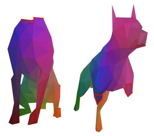
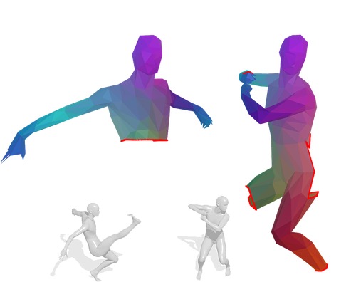
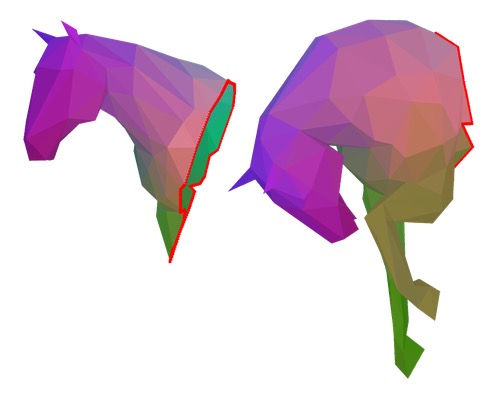
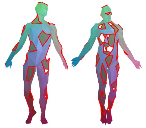
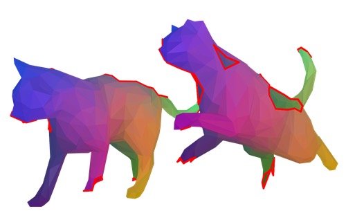
Figure 7: Our method can handle the difficult case of matching pairs of partial shapes without availability of complete shapes, in which the orientation-preserving diffeomorphism serves as powerful constraint (boundaries are shown as red lines). (Best viewed magnified on screen)

$0$$0.5$$1$$0$$50$$100$SHREC’19

$\uparrow$$0.836$$0.910$