Magnetohydrodynamic Turbulence: Chandrasekhar’s Contributions & Beyond

Abstract

In the period of 1948-1955, Chandrasekhar wrote four papers on magnetohydrodynamic (MHD) turbulence, which are the first set of papers in the area. The field moved on following these pioneering efforts. In this paper, I will briefly describe important works of MHD turbulence, starting from those by Chandrasekhar.

mkv@iitk.ac.in

12.3456/s78910-011-012-3 #### 000 0000 1– 1

1 Introduction

Chandrasekhar pioneered the following areas of astrophysics: white dwarfs, neutron stars, black holes, stellar structures, radiative transfers, random processes, stability of ellipsoidal figures of equilibrium, instabilities, and turbulence. His work on turbulence is not as well known as others, even though his papers on quantification of structure functions and energy spectrum of magnetohydrodynamic (MHD) turbulence are first ones in the field. Recently, Sreenivasan (2019) wrote a very interesting review on Chandrasekhar’s contributions to fluid mechanics, which includes hydrodynamic instabilities and turbulence. While Sreenivasan’s article is focussed on hydrodynamics, in this paper, I will provide a brief review on Chandrasekhar’s work in MHD turbulence.

In the years 1948 to 1960, Chandrasekhar worked intensely on turbulence. In 1954, Chandrasekhar gave a set of lectures on turbulence in Yerkes Observatory. These lectures, published by Spiegel (2011), illustrate Chandrasekhar’s line of approach to understand turbulence. To quote Spiegel (2011), “Still, Chandra pulled things together and published two papers on his approach (in 1955 and 1956). The initial reception of the theory was positive. Indeed, Stanley Corrsin once told me that, back in the mid-fifties, he was so sure that the ‘turbulence problem’ would soon be solved that he bet George Uhlenbeck five dollars that he was right. Afterwards, when Corrsin and Uhlenbeck heard Chandra lecture on his theory, Uhlenbeck came over and handed Corrsin a fiver. It soon appeared that Uhlenbeck should have waited before parting with his money.” Refer to Sreenivasan (2019) for a more detailed account of Chandrasekhar’s work on turbulence and instabilities. The books by Wali (1991) and Miller (2007) are excellent biographies of Chandrasekhar.

In this paper, I provide a brief overview of the leading works in MHD turbulence, starting from those of Chandrasekhar. These works are related to the inertial range of homogeneous MHD turbulence. The works beyond Chandrasekhar’s contributions are divided in two periods: (a) 1965-1990, during which the field was essentially dominated by the belief that Kraichnan-Iroshnikov model works for MHD turbulence. (b) 1991-2010, during which many models and theories came up that support Kolmogorov-like spectrum for MHD turbulence. I also remark that the present paper is my personal perspective that may differ from those of others.

The outline of the paper is as follows: In Section 2, I will briefly introduce the theories of hydrodynamic turbulence by Kolmogorov and Heisenberg. Section 3 contains a brief summary of Chandrasekhar’s work on MHD turbulence that occurred between 1948 and 1955. In Sections 4 and 5, I will brief works on MHD turbulence during the periods 1965-1990 and 1991-2010 respectively. Section 6 contains a short discussion on possible approaches for resolving the present impasse in MHD turbulence. I conclude in Section 7.

2 Leading turbulence models before Chandrasekhar’s work

Chandrasekhar worked on hydrodynamic (HD) and magnetohydrodynamics (MHD) turbulence during the years 1948 to 1960. Some of the papers written by him during this period are Chandrasekhar (1950, 1951a, 1951b, 1952, 1955a, 1955b, 1956). In addition, Chandrasekhar (1961) wrote a famous treatise on hydrodynamic and magnetohydrodynamic instabilities. Chandrasekhar’s lectures on turbulence (delivered in 1954) have been published by Spiegel (2011). Refer to Sreenivasan (2019) for commentary on these works.

During or before Chandrasekhar’s work, there were important results by Taylor, Batchelor, Kolmogorov, Heisenberg, among others. Here, we briefly describe the turbulence theories of Kolmogorov and Heisenberg, primarily because Chandrasekhar’s works on MHD turbulence are related to these theories. We start with Kolmogorov’s theory of turbulence.

2.1 Kolmogorov’s theory of turbulence

Starting from Navier-Stokes equation, under the assumptions of homogeneity and isotropy, Kármán & Howarth (1938) [also see Monin & Yaglom (2007)] derived the following evolution equation for $\left\langle u_{i}u^{\prime}_{i}\right\rangle$:

$$\frac{\partial}{\partial t}\frac{1}{2}\left\langle u_{i}u_{i}^{\prime}\right\rangle = \frac{1}{4}\nabla_{l}\cdot\left\langle|{\bf u^{\prime}-u}|^{2}({\bf u^{\prime}-u})\right\rangle+\left\langle F_{\mathrm{LS},i}u_{i}^{\prime}\right\rangle$$ (1)

$$+\nu\nabla^{2}\left\langle u_{i}u_{i}^{\prime}\right\rangle$$

$$= T_{u}({\bf l})+\mathcal{F}_{\mathrm{LS}}({\bf l})-D_{u}({\bf l}),$$

where u and u’ are the velocities at the locations r and r+l respectively, and $\nu$ is the kinematic viscosity (see Figure 1). The terms $T_{u}({\bf l})$ and $D_{u}({\bf l})$ represent respectively the nonlinear energy transfer and the dissipation rates at scale l, while $\mathcal{F}_{\mathrm{LS}}({\bf l})$ is the energy injection rate by the external force $\mathbf{F}_{\mathrm{LS}}$, which is active at large scales. For a steady turbulence, under the limit $\nu\rightarrow 0$, Kolmogorov (1941b, a) showed that in the inertial range (intermediate scales between the forcing and dissipation scales),

$$\left\langle[{\bf(u^{\prime}-u)}\cdot\hat{\bf l}]^{3}\right\rangle=-\frac{4}{5}\epsilon_{u}l,$$ (2)

where $\epsilon_{u}$ is the viscous dissipation rate per unit mass, and $\hat{\bf l}$ is the unit vector along l. Kolmogorov’s theory is commonly referred to as K41 theory.

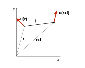
Figure 1: The velocity fields at two points r and r+l are u(r) and u(r+l) respectively. We denote them using u and u’ respectively.

A simple-minded extrapolation of Eq. (2) leads to

$$\left\langle[{\bf(u^{\prime}-u)}\cdot\hat{\bf l}]^{2}\right\rangle\approx\epsilon_{u}^{2/3}l^{2/3}$$ (3)

whose Fourier transform leads to the following formula for the energy spectrum:

$$E(k)=K_{\mathrm{Ko}}\epsilon_{u}^{2/3}k^{-5/3},$$ (4)

where $K_{\mathrm{Ko}}$ is a nondimensional constant [Frisch (1995)].

In Fourier space, Eq. (1) transforms to the following energy transfer relation (Verma (2019, 2022)):

$$\frac{\partial}{\partial t}E_{u}({\bf k},t)=T_{u}({\bf k},t)+\mathcal{F}_{\mathrm{LS}}({\bf k},t)-D_{u}({\bf k},t),$$ (5)

where $E_{u}({\bf k})=|{\bf u(k)}|^{2}/2$ is the modal energy, and

$$T_{u}({\bf k},t)=\sum_{\bf p}\Im[\{{\bf k\cdot u(q)}\}\{{\bf u(p)\cdot u^{*}(k)}\}],$$ (6)

with ${\bf q=k-p}$, represents the total energy gained by ${\bf u(k)}$ via nonlinear energy transfers. For isotropic turbulence,

$$T_{u}({\bf k})=T_{u}(k)=-\frac{d}{dk}\Pi_{u}(k),$$ (7)

where $\Pi_{u}(k)$ is the energy flux emanating from a wavenumber sphere of radius $k$. In the inertial range, the energy injection by the external force vanishes and viscous dissipation rate is negligible, hence $\Pi_{u}(k)\approx\mathrm{const}$. Refer to Frisch (1995), Verma (2019), and Verma (2022) for more details.

2.2 Heisenberg’s theory of turbulence

In this subsection, we describe Heisenberg’s theory of turbulence because Chandrasekhar employed this theory to derive the energy spectrum for MHD turbulence. Heisenberg (1948) derived an integral equation for the temporal evolution of kinetic energy spectrum $E_{u}(k)$ under the assumption of homogeneity and isotropy. In particular, he derived that

$$\frac{\partial}{\partial t}\int_{0}^{k}dk^{\prime}E_{u}(k^{\prime},t) = -2\left(\nu+\alpha\int_{k}^{\infty}\sqrt{\frac{E_{u}(k^{\prime})}{k^{\prime 3}}}dk^{\prime}\right)$$ (8)

$$\times\int_{0}^{k}k^{\prime 2}E_{u}(k^{\prime})dk^{\prime}.$$

In the above equation, the second term of the right-hand-side is a model for the diffusion of kinetic energy to smaller scales by eddy viscosity (induced by the nonlinear term). Many authors, including Chandrasekhar, have employed Heisenberg’s model for modelling turbulent flows.

3 Chandrasekhar’s contributions to MHD turbulence

Chandrasekhar wrote around a dozen papers on turbulence, four of which are on MHD. He focussed on the closing the hierarchical equations of turbulence. In the following, I will provide a brief overview of Chandrasekhar’s work on MHD turbulence.

In turbulence, the nonlinear interactions induce energy transfers among the Fourier modes. Hydrodynamic interactions involve triadic interactions, e.g., in Eqs. (5,6), the Fourier mode ${\bf u(k)}$ receives energy from the Fourier modes ${\bf u(p)}$ and ${\bf u(q)}$. In 1954, Chandrasekhar gave a set of lectures on turbulence in which he showed that the energy transfer from ${\bf u(p)}$ to ${\bf u(k)}$ with the mediation of ${\bf u(q)}$ is

$$Q({\bf k,k^{\prime}})=\Im[({\bf u({q})\cdot k})({\bf u{(p})\cdot u^{*}({k})})].$$ (9)

As far as we know, the above formula first appears in Onsager (1949), but not in any paper of Chandrasekhar. Incidently, Onsager is not cited for this formula in Spiegel (2011). Hence, it is not apparent whether Chandrasekhar derived Eq. (9) independently, or he was aware of Onsager’s work. Around 2000, we were working on the energy fluxes of MHD turbulence, and we (Dar $et~{}al$. (2001)) arrived at the same formula independently. Note that in MHD turbulence, energy transfers occur between velocity field and magnetic field as well.

Let us get back to MHD turbulence. Chandrasekhar’s four papers on MHD turbulence are as follows:

1. Chandrasekhar (1951a): The invariant theory of isotropic turbulence in magneto-hydrodynamics

2. Chandrasekhar (1951b): The Invariant Theory of Isotropic Turbulence in Magneto-Hydrodynamics. II

3. Chandrasekhar (1955a): Hydromagnetic turbulence. I. A deductive theory

4. Chandrasekhar (1955b): Hydromagnetic turbulence II. An elementary theory

The first three papers are in real space, and they are generalization of the hydrodynamics equations of Kármán & Howarth (1938) and Kolmogorov (1941a, b) to MHD turbulence. The fourth paper attempts to employ Heisenberg’s theory of turbulence to MHD turbulence (in spectral space). In the following discussion, we briefly sketch the results of these papers.

3.1 Summary of the results of Chandrasekhar (1951a, b) and Chandrasekhar (1955a)

For isotropic and homogeneous MHD turbulence, Chandrasekhar (1951a) derived equations for the second-order correlations of the velocity and magnetic fields. The derivation here is along the lines followed by Kármán & Howarth (1938). Note that the equations for MHD turbulence are much more complex due to more number of fields and nonlinear terms than in HD turbulence. As in other papers, Chandrasehkar follows rigorous and formal approach in these papers. We skip the details due to their lengths and complexity, and provide only the leading equations of the papers.

The second-order correlation functions for the velocity and magnetic fields are given below:

$$\left\langle u_{i}u_{j}^{\prime}\right\rangle=\frac{Q^{\prime}}{l}l_{i}l_{j}-(lQ^{\prime}+2Q)\delta_{ij},$$ (10)

$$\left\langle b_{i}b_{j}^{\prime}\right\rangle=\frac{H^{\prime}}{l}l_{i}l_{j}-(lH^{\prime}+2H)\delta_{ij}.$$ (11)

Here, b is the magnetic field, and $u_{j},b^{\prime}_{j}$ represent the $j$th components of the velocity and magnetic fields at the locations r and r+l respectively. Throughout the paper, the magnetic field is in velocity units, which is obtained by dividing b in CGS unit with $\sqrt{4\pi\rho}$, where $\rho$ is the density of the fluid. Note that the above correlation functions satisfy the incompressibility relations, $\partial^{\prime}_{j}\left\langle u_{i}u_{j}^{\prime}\right\rangle=0$ and $\partial^{\prime}_{j}\left\langle b_{i}b_{j}^{\prime}\right\rangle=0$.

As a sample, we present one of the equations derived by Chandrasekhar (1951b):

$$\frac{\partial}{\partial l_{m}}\left\langle(b_{i}u_{m}-b_{m}u_{i})b_{j}^{\prime}\right\rangle = \frac{\partial}{\partial l_{m}}P(l_{i}\delta_{jm}-l_{m}\delta_{ij})$$ (12)

$$= \frac{P^{\prime}}{r}l_{i}l_{j}-(lP^{\prime}+2P)\delta_{ij}$$

where $P$ is a scalar function, similar to $Q$ and $H$ of Eqs. (10, 11). Using the above equations and others, one of the inertial-range relations derived by Chandrasekhar is

$$\left\langle(u_{1}^{2}+2b_{2}^{2})u_{1}^{\prime}\right\rangle=-\frac{2}{15}\epsilon r,$$ (13)

where $\epsilon$ is the total dissipation rate, and $u_{1},b_{1}$ are the longitudinal components along $\hat{\bf l}$, while $u_{2},b_{2}$ are components perpendicular to $\hat{\bf l}$. The above equation is a generalization of K41 relation to MHD turbulence.

For hydrodynamic turbulence, Loitsiansky (1939) derived the following relations:

$$\int_{0}^{\infty}Q(l)l^{4}dl=\mathrm{const.}$$ (14)

where $Q(l)$ is the correlation function defined in Eq. (10). Using the dynamical equations of MHD, Chandrasehkar showed that Loitsiansky’s integral remains constant to MHD turbulence as well. In the second paper (Chandrasekhar (1951b)), Chandrasekhar derived relations for the third-order correlation functions $\left\langle pu_{i}^{\prime}u_{j}^{\prime}\right\rangle$ and $\left\langle pb_{i}^{\prime}b_{j}^{\prime}\right\rangle$, where $p$ is the pressure field.

In Chandrasekhar (1955a), Chandrasekhar derived a pair of differential equations for the velocity and magnetic fields at two different points and at two different times in terms of scalars. The derivation is quite mathematical and detailed, and is being skipped here.

3.2 Summary of the results of Chandrasekhar (1955b)

Chandrasekhar (1955b) generalized Heisenberg’s theory for hydrodynamic turbulence to MHD turbulence. In this paper, the equations are in spectral space. One of the leading equations of the paper is

$$-\frac{\partial}{\partial t}\int_{0}^{k}dk^{\prime}[E_{u}(k^{\prime},t)+E_{b}(k^{\prime},t)]$$ (15)

$$= 2[\nu\int_{0}^{k}k^{\prime 2}E_{u}(k^{\prime})dk^{\prime}+\eta\int_{0}^{k}k^{\prime 2}E_{b}(k^{\prime})dk^{\prime}]$$

$$+\kappa\int_{k}^{\infty}\left[\sqrt{\frac{E_{u}(k^{\prime})}{k^{\prime 3}}}+\sqrt{\frac{E_{b}(k^{\prime})}{k^{\prime 3}}}\right]\times$$

$$\int_{0}^{k}k^{\prime 2}[E_{u}(k^{\prime})+E_{b}(k^{\prime})]dk^{\prime},$$

where $E_{u}(k),E_{b}(k)$ are the energy spectra of the velocity and magnetic fields respectively, $\eta$ is the magnetic diffusivity, and $\kappa$ is a constant. Physical interpretation of Eq. (15) is as follows. Without an external force, the energy lost by all the modes of a wavenumber sphere of radius $k$ is by (a) viscous and Joule dissipation in the sphere (the first term in the right-hand-side of Eq.(15)), and (b) the nonlinear energy transfer from the modes inside the sphere to the modes outside the sphere (the second term in the right-hand-side of Eq.(15)). The latter term is the total energy flux (Verma (2004, 2019)).

Using the above equation, Chandrasekhar derived several results for the asymptotic cases, e.g., $\nu\rightarrow 0$ and $\eta\rightarrow 0$. For example, Chandrasekhar observed that for small wavenumbers ($k\rightarrow 0$), the velocity and magnetic fields are nearly equipartitioned, and they exhibit Kolmogorov’s energy spectrum ($k^{-5/3}$ ). However, at large wavenumbers, the magnetic and kinetic energies are not equipartitioned. Quoting from his paper, “in the velocity mode (kinetic-energy dominated case), the ratio of the magnetic energy to the kinetic energy tends to zero among the smallest eddies present (i.e., as $k\rightarrow\infty$), while in the magnetic mode (magnetic-energy dominated case), the same ratio tends to about 2.6 as $k\rightarrow\infty$.”

Chandrasekhar (1951a, b) and Chandrasekhar (1955a, b) are the first set of papers on MHD turbulence. However, after these pioneering works, Chandrasekhar left the field somewhat abruptly. Sreenivasan (2019) ponders over this question in his review article.

A decade later, Kraichnan (1965) and Iroshnikov (1964) brought next breakthroughs in MHD turbulence. Thus, Chandrasekhar pioneered the field of MHD turbulence. We find that Chandrasekhar’s results have not been tested rigorously using numerical simulations and solar wind observations, and they have received less attention than his other papers. In the following discussion, we will briefly discuss some of the important papers after Chandrasekhar’s work on MHD turbulence.

4 Works in MHD turbulence between 1965 and 1990

4.1 The energy spectrum $k^{-3/2}$: Kraichnan and Iroshnikov

In the presence of a mean magnetic field (${\bf B}_{0}$), MHD has two kinds of Alfvén waves that travel parallel and antiparallel to the mean magnetic field. Kraichnan (1965) and Iroshnikov (1964) exploited this observation and argued that the Alfvén time scale is the relevant time scale for MHD turbulence. Consequently, the interaction time for an Alfvén wave of wavenumber $k$ is proportional to $(kB_{0})^{-1}$. Note that the magnetic field including ${\bf B}_{0}$ is in velocity units.

Using these inputs and dimensional analysis, Kraichnan (1965) and Iroshnikov (1964) argued that the kinetic and magnetic energies are equipartitioned, and that the magnetic energy spectrum is

$$E_{b}(k)=A(\epsilon B_{0})^{1/2}k^{-3/2},$$ (16)

where $A$ is a dimensionless constant. The above phenomenology predicts $k^{-3/2}$ energy spectrum that differs from Kolmogorov’s $k^{-5/3}$ spectrum, for which the relevant time scale is $(ku_{k})^{-1}$. Note however that the solar wind turbulence tends to exhibit $k^{-5/3}$ spectrum [e.g., Matthaeus & Goldstein (1982)], however some authors report $k^{-3/2}$ spectrum for the solar wind.

4.2 Generalization by Dobrowolny $et~{}al$. (1980)

The MHD equations can be written in terms of Elsässer variables $\bf{z}^{\pm}={\bf u}\pm{\bf b}$. These variables represent the amplitudes of the Alfvén waves travelling in the opposite direction. The nonlinear interactions between the Alfvén waves yield energy cascades. The fluxes of $\bf{z}^{+}$ and $\bf{z}^{-}$ are $\epsilon_{z^{+}}$ and $\epsilon_{z^{-}}$ respectively, which are also their respective dissipation rates.

Dobrowolny $et~{}al$. (1980) modelled the random scattering of Alfvén waves. They showed that the two fluxes are equal irrespective of the ratio $z^{+}/z^{-}$, i.e.,

$$\epsilon_{z^{+}}=\epsilon_{z^{-}}.$$ (17)

Dobrowolny $et~{}al$. (1980) used these observations to explain depletion of cross helicity in the solar wind as it moves away from the Sun. Also, they derived $k^{-3/2}$ energy spectrum for ${\bf z}^{\pm}$, as in Eq. (16).

4.3 Field-theoretic calculation

Fournier $et~{}al$. (1982) employed field-theoretic methods to derive energy spectra $E_{u}(k)$ and $E_{b}(k)$, and the cross helicity spectrum $H_{c}(k)$. They employed the renormalization group procedure of Yakhot & Orszag (1986). The authors attempted to compute the renormalized viscosity and magnetic diffusivity, as well as vortex corrections. However, they were short of closure due to the complex nonlinear couplings of MHD turbulence. There are more field-theoretic works before 1990, but I am not describing them here due to lack of space.

Kraichnan and Iroshnikov’s models dominated till 1990. During this period, numerical simulations tended to support the $k^{-3/2}$ spectrum [e.g., see Biskamp $et~{}al$. (1989)], but they were not conclusive due to lower resolutions. On the contrary, several solar wind observations [e.g., Matthaeus & Goldstein (1982)] supported Kolmogorov’s spectrum. In 1990’s, new models and theories were constructed that support Kolmogorov’s spectrum for MHD turbulence. We describe these theories in the next section.

5 Works between 1991 and 2010

As discussed earlier, Chandrasekhar (1955b) argued that the kinetic and magnetic energy follow $k^{-5/3}$ spectrum as $k\rightarrow 0$. More detailed works on Kolmogorov’s spectrum for MHD turbulence followed after this work.

5.1 Emergence of $k^{-5/3}$ in MHD turbulence: Marsch (1991)

Marsch (1991) considered a situation when the Alfvénic fluctuations are much larger than the mean magnetic field. In this case, the nonlinear term (${\bf z}^{\mp}\cdot\nabla{\bf z}^{\pm}$) dominates the linear term (${\bf B}_{0}\cdot\nabla{\bf z}^{\pm}$). Here, usual dimensional arguments yields

$$\frac{E_{z^{+}}(k)}{E_{z^{-}}(k)}=\frac{K_{+}}{K_{-}}\left(\frac{\epsilon_{z^{+}}}{\epsilon_{z^{-}}}\right)^{2},$$ (18)

where $K_{\pm}$ are dimensionless constants. Note that the inertial-range fluxes $\epsilon_{z^{+}}$ and $\epsilon_{z^{-}}$ are unequal, unlike the predictions of Dobrowolny $et~{}al$. (1980) (see Eq. (17)). The inequality increases with the increase of the ratio $E_{z^{+}}(k)/E_{z^{-}}(k)$.

Interestingly, the formulation of Dobrowolny $et~{}al$. (1980) too yields $k^{-5/3}$ spectrum when the Alfvén time is replaced by nonlinear time scale $(ku_{k})^{-1}$ (Verma (2004)). Matthaeus & Zhou (1989) attempted to combine the $k^{-3/2}$ and $k^{-5/3}$ models by proposing the harmonic mean of the Alfvén time scale and the nonlinear time scale as the relevant time scale. In their framework, $E(k)\sim k^{-5/3}$ for small wavenumbers, and $E(k)\sim k^{-3/2}$ for larger wavenumbers. It turns out that the predictions of Matthaeus & Zhou (1989) are counter to weak turbulence theories where $E(k)\sim k^{-3/2}$ should be active at small wavenumbers.

5.2 Energy fluxes: Verma et al. [1994, 1996]

For my Ph. D. thesis (Verma (1994)), I wanted to verify which of the two spectra, $k^{-5/3}$ and $k^{-3/2}$, is valid for MHD turbulence. We simulated several two-dimensiona (2D) MHD flows on $512^{2}$ grids, and a single 3D flow on $128^{3}$ grid. These runs had different $B_{0}$ and $z^{+}/z^{-}$. We observed that the energy fluxes $\epsilon_{z^{\pm}}$ satisfy Eq. (18) even when $B_{0}$ is five times larger than the fluctuations, and that the fluxes deviate significantly from Eq. (17). Based on these observations, we concluded that Kolmogorov’s model is more suited for MHD turbulence than Iroshnikov-Kraichnan model (Verma (1994); Verma $et~{}al$. (1996)).

5.3 Politano & Pouquet (1998) on structure functions

Following similar approach as K41, Politano & Pouquet (1998) showed that for MHD turbulence, the third-order structure function follows

$$\left\langle({\bf z^{\prime\pm}-z^{\pm}})^{2}[({\bf z^{\prime\mp}}-{\bf z^{\mp}})\cdot\hat{l}]\right\rangle=-\frac{4}{3}\epsilon_{z^{\pm}}l.$$ (19)

The above equations have a simple form because of the absence of cross transfer between ${\bf z}^{+}$ and ${\bf z}^{-}$. Note that the energy fluxes $\Pi_{z^{\pm}}$ are constant in the inertial range (Verma (2019)). The above relations translate to Kolmogorov’s spectrum in Fourier space.

Politano & Pouquet (1998) also derived the third-order structure functions for the velocity and magnetic fields. These relations are more complex due to the coupling between the velocity and magnetic fields. Also refer to the complex relations in Chandrasekhar (1951a), which differ from those of Politano & Pouquet (1998).

5.4 Anisotropic MHD turbulence

Kolmogorov’s $k^{-5/3}$ theory and Iroshnikov-Kraichnan’s $k^{-3/2}$ theory assume the flow to be isotropic. However, this is not the case in MHD turbulence when a mean magnetic field is present. There are several interesting results for this case, which are discussed below.

5.4.1 Goldreich & Sridhar (1995):

For anisotropic MHD turbulence, Goldreich & Sridhar (1995) argued that a critical balance is established between the Alfvén time scale and nonlinear time scale, that is, $k_{\parallel}B_{0}\approx k_{\perp}z^{\pm}_{k_{\perp}}$. Using this assumption, Goldreich and Sridhar (1995) derived that

$$E(k_{\perp})=\epsilon^{2/3}k_{\perp}^{-5/3},$$ (20)

which is Kolmogorov’s spectrum.

5.4.2 Weak turbulence formalism:

For MHD turbulence with strong ${\bf B}_{0}$, Galtier $et~{}al$. (2000) constructed a weak turbulence theory and obtained

$$\epsilon\sim\frac{1}{k_{\parallel}B_{0}}E_{z^{+}}(k_{\perp})E_{z^{-}}(k_{\perp})k_{\perp}^{4}.$$ (21)

When ${\bf z}^{+}$ and ${\bf z}^{-}$ have the same energy spectra, Eq. (21) reduces to

$$E(k_{\perp},k_{\parallel})\sim B_{0}^{1/2}k_{\perp}^{1/2}k_{\perp}^{-2}.$$ (22)

Several numerical simulations support this prediction. Note however that the solar wind turbulence exhibits nearly $k^{-5/3}$ energy spectrum even though its fluctuations are five times weaker than the Parker field. This aspect needs a careful look.

5.4.3 Anistropic energy spectrum and fluxes:

In the presence of strong ${\bf B}_{0}$, the energy spectrum and energy transfers become anisotropic. Teaca $et~{}al$. (2009) quantified the angular dependence of energy spectrum using ring spectrum. They showed that for strong ${\bf B}_{0}$, the energy tends to concentrate near the equator, which is the region perpendicular to ${\bf B}_{0}$. Teaca $et~{}al$. (2009) and Sundar $et~{}al$. (2017) also studied the anisotropic energy transfers using ring-to-ring energy transfers. In addition, Sundar $et~{}al$. (2017) showed that strong magnetic field yields an inverse cascade of kinetic energy which may invalidate some of the assumptions made in Goldreich & Sridhar (1995) and in Galtier $et~{}al$. (2000).

5.5 Mean magnetic field renormalization

Given that several solar wind observations, numerical simulations, and the works of Politano & Pouquet (1998) support $k^{-5/3}$ spectrum, it is quite puzzling what is going wrong with Kraichnan and Iroshnikov’s arguments on the scattering of Alfvén waves. This led me to think about the effects of magnetic fluctuations on the propagation of Alfvén wave.

In the presence of a mean magnetic field, MHD equations are nearly linear at large length scales. Alfvén waves are the basic modes of the linearlized MHD equations. However, the nonlinear term becomes significant at the intermediate and small scales (large wavenumbers). Using renormalization group (RG) procedure, I could show that the an Alfvén wave with wavenumber k is affected by an “effective” mean magnetic field, which is the renormalized mean magnetic field (Verma (1999, 2004)):

$$B_{0}(k)=C\epsilon^{1/3}k^{-1/3},$$ (23)

where $C$ is a constant. Hence, an Alfvén wave is not only affected by the mean magnetic field, but also by the waves with wavenumber near k; this feature is called local interaction. See Figure 2 for an illustration. Note that Kraichnan (1965) and Iroshnikov (1964) considered time scales based only on the mean magnetic field.

Figure 2: A schematic diagram of multiscale Alfvén waves. A fluctuation of wavelength $\lambda_{1}$ is affected by the “effective” or renormalized magnetic field $B_{0}(k=1/\lambda_{1})$ that scales as $k^{-1/3}$. Reproduced with permission from Verma (2019).

Substitution of $B_{0}(k)$ of Eq. (23) in Eq. (16) yields

$$E_{u}(k)\approx[\epsilon B_{0}(k)]^{1/2}k^{-3/2}\approx\epsilon^{2/3}k^{-5/3}.$$ (24)

Thus, we recover Kolmogorov’s spectrum in the framework of Kraichnan and Iroshnikov. Hence, there is consistency among various models. This argument is complimentary to those of Goldreich & Sridhar (1995).

In the RG procedure of Verma (1999), I went from large scales to small scales because the nonlinear interaction in MHD turbulence is weak at large scales. This is akin to quantum electrodynamics (QED) where particles (consider electrons) are free when they are separated by large distances.

5.6 Renormalization of viscosity and magnetic diffusivity

In the usual RG procedure of turbulence, we coarse grain the small-scale fluctuations (Yakhot & Orszag (1986), McComb (1990)). That is, we average the small-scale fluctuations and go to larger scales. At small scales, the linearized MHD equations have viscous and magnetic-diffusive terms. As we go to larger scales, the nonlinear terms enhance diffusion, which is referred to as turbulent diffusion. The effective diffusive constants in MHD turbulence are the renormalized kinematic viscosity and renormalized magnetic diffusivity.

In Verma (2001), Verma (2003b), Verma (2003a), and Verma (2004), I implemented the above scheme using the self-consistent procedure of McComb (1990, 2014), and computed the renormalized viscosity and magnetic diffusivity. This self-consistent procedure was useful in circumventing the difficulties faced by Fournier $et~{}al$. (1982) and others. Compared to the procedure of Yakhot & Orszag (1986), McComb’s scheme has less parameters to renormalize. For tractability, I focussed on the following two limiting cases:

5.6.1 Cross helicity $H_{c}=0$:

This assumption leads to major simplification of the calculation. I could show that

$$\nu(k) = \sqrt{K}\nu_{*}\epsilon^{1/3}k^{{}_{4}/3},$$ (25)

$$\eta(k) = \sqrt{K}\eta_{*}\epsilon^{1/3}k^{-4/3},$$ (26)

$$E(k) = K\epsilon^{2/3}k^{-5/3}$$ (27)

are consistent solutions of RG equations. Thus, we show that the kinetic and magnetic energies exhibit $k^{-5/3}$ energy spectra.

5.6.2 Non-Alfvénic case, $z^{+}\gg z^{-}$:

This limiting case corresponds to large cross helicity. Again, a self-consistent RG procedure yields $k^{-5/3}$ spectrum for the Elsässer variables.

5.7 Boldyrev (2006) revives $k^{-3/2}$ spectrum

Boldyrev (2006) hypothesized that the inertial-range fluctuations of MHD turbulence have certain dynamical alignments that yields interaction time scale as

$$T_{k}\sim(ku_{k}\sin\theta_{k})^{-1}\sim(ku_{k}\theta_{k})^{-1},$$ (28)

where $\theta_{k}$ is the angle between the velocity and magnetic fluctuations at the scale of $k^{-1}$. Boldyrev (2006) argued that $\theta_{k}\sim k^{-1/4}$. Using dimensional analysis, we obtain

$$\theta_{k}\sim k^{-1/4}(\epsilon/B_{0}^{3})^{1/4},$$ (29)

substitution of which in the flux equation yields

$$\Pi\sim\epsilon\sim\frac{u_{k}^{2}}{T_{k}}\sim ku_{k}^{3}k^{-1/4}(\epsilon/B_{0}^{3})^{1/4}.$$ (30)

The above equation was inverted to obtain the following energy spectrum:

$$E_{u}(k)\sim(\epsilon B_{0})^{1/2}k^{-3/2},$$ (31)

which is same as that predicted by Kraichnan (1965) and Iroshnikov (1964). Boldyrev and coworkers performed numerical simulations and observed consistency with the above predictions. Thus, $k^{-3/2}$ spectrum has come back with vengeance.

5.8 Energy fluxes of MHD turbulence

MHD turbulence has six energy fluxes, in contrast to single flux of hydrodynamic turbulence (Dar $et~{}al$. (2001); Verma (2004); Debliquy $et~{}al$. (2005)). The energy fluxes from the velocity field to the magnetic field are responsible for dynamo action, or amplification of magnetic field in astrophysical objects (Brandenburg & Subramanian (2005); Kumar $et~{}al$. (2015); Verma & Kumar (2016)). Energy fluxes can also help us decipher the physics of MHD turbulence, e.g., in Verma $et~{}al$. (1996). We cannot describe details of energy flux in this short paper; we refer the reader to Verma (2004); Brandenburg & Subramanian (2005); and Verma (2019) for details.

6 Possible approaches to reach the final theory of MHD turbulence

As discussed above, we are far from the final theory of MHD turbulence. Future high-resolution simulations and data from space missions may help resolve this long-standing problem. I believe that the following explorations would provide important clues for MHD turbulence:

1. Measurements of the time series of the inertial-range Alfvén waves would help us explore the wavenumber dependence of $B_{0}$ (Verma (1999)).

2. The energy fluxes of ${\bf z^{\pm}}$, $\epsilon_{z^{\pm}}$, are approximately equal in the Iroshnikov-Kraichnan phenomenology, but not so in Kolmgoorov-like phenomenology for MHD turbulence. Verma $et~{}al$. (1996) showed that $\epsilon_{z^{\pm}}$ for 2D MHD turbulence follow Kolmogorov-like theory. But, we need to extend this study to three dimensions and for high resolutions. The findings through these studies will also help estimate the turbulent heating in the solar wind and in the solar corona.

3. Recent spacecrafts are providing high-resolution solar wind and corona data, which can be used for investigating MHD turbulence. These studies would compliment numerical studies.

We hope that above studies would be carried out in near future, and we will have a definitive theory of MHD turbulence soon.

7 Summary

In this paper, I surveyed the journey of MHD turbulence, starting from the pioneering works of Chandrasekhar. Chandrasekhar attempted to model the structure functions and energy spectra of MHD turbulence. Unfortunately, Chandrasekhar’s papers on hydrodynamic and hydromagnetic turbulence did not attract significant attention in the community. Sreenivasan (2019), who studied this issue in detail, points out the following possible reasons for the above. Chandrasekhar’s papers are typically more mathematical than a typical paper on turbulence. As written in Sreenivasan (2019), “what mattered to Chandra was what the equations revealed; everything else was superstition and complacency.” Thus, Chandrasekhar did not make significant effort to extract physics from mathematical equations, unlike the other stalwarts of the field (e.g., Batchelor, Taylor, Kolmogorov).

Sreenivasan (2019) points out another factor that drifted Chadrasekhar from the turbulence community. Chandrasekhar sent one of his important manuscripts on turbulence to the Proceedings of Royal Society, but the paper was rejected. This paper was eventually published in Physical Review (Chandrasekhar (1956)), but it contained several incorrect assumptions (Sreenivasan (2019)). When these assumptions were criticised by Kraichnan and others, Chandrasekhar did not take them kindly and left the field of turbulence abruptly. Refer to Sreenivasan (2019) for details on this topic.

More work on MHD turbulence followed 10 years after Chandrasekhar left this field. I divided these works in two temporal regimes: between 1965 to 1990, and between 1991 to 2010. The first period was dominated by Kraichnan and Iroshnikov’s $k^{-3/2}$ model, which is based on the scattering of Alfvén waves. Till 1990, the community appears to believe in the validity of this theory, even though several astrophysical observations supported $k^{-5/3}$ spectrum. From 1991 onwards, there were a flurry of models and calculations that support Kolmogorov-like spectrum ($k^{-5/3}$) for MHD turbulence. However, in 2006, Boldyrev and coworkers argued in favour of $k^{-3/2}$ spectrum. Hence, the jury is not yet out. More detailed diagnostics have to be performed to arrive at the final theory of MHD turbulence.

At present, there is a lull in this fields. We hope that in near future, we will be able to completely understand the underlying physics of MHD turbulence, a journey that started with Chandrasekhar’s pioneering work.

References

- Biskamp . (1989) Biskamp, D., Biskamp, D., & Welter, H. 1989, Phys. Fluids B, 1, 1964
- Boldyrev (2006) Boldyrev, S. 2006, Phys. Rev. Lett., 96, 115002
- Brandenburg & Subramanian (2005) Brandenburg, A., & Subramanian, K. 2005, Phys. Rep., 417, 1
- Chandrasekhar (1950) Chandrasekhar, S. 1950, Phil. Trans. R. Soc. A, 242, 557
- Chandrasekhar (1951a) —. 1951a, Proc. R. Soc. A, 204, 435
- Chandrasekhar (1951b) —. 1951b, Proc. R. Soc. A, 207, 301
- Chandrasekhar (1952) —. 1952, Phil. Trans. R. Soc. A, 244, 357
- Chandrasekhar (1955a) —. 1955a, Proceedings of the Royal Society of London. Series A. Mathematical and Physical Sciences, 233, 322
- Chandrasekhar (1955b) —. 1955b, Proceedings of the Royal Society of London. Series A. Mathematical and Physical Sciences, 233, 330
- Chandrasekhar (1956) —. 1956, Physical Review, 102, 941
- Chandrasekhar (1961) —. 1961, Hydrodynamic and Hydromagnetic Stability (Clarendon: Oxford University Press)
- Dar . (2001) Dar, G., Verma, M. K., & Eswaran, V. 2001, Physica D, 157, 207
- Debliquy . (2005) Debliquy, O., Verma, M. K., & Carati, D. 2005, Phys. Plasmas, 12, 042309
- Dobrowolny . (1980) Dobrowolny, M., Mangeney, A., & Veltri, P. 1980, Phys. Rev. Lett., 45, 144
- Fournier . (1982) Fournier, J. D., Sulem, P. L., & Pouquet, A. 1982, J. Phys. A: Math. Theor., 15, 1393
- Frisch (1995) Frisch, U. 1995, Turbulence: The Legacy of A. N. Kolmogorov (Cambridge: Cambridge University Press)
- Galtier . (2000) Galtier, S., Nazarenko, S. V., Newell, A. C., & Pouquet, A. G. 2000, J. Plasma Phys., 63, 447
- Goldreich & Sridhar (1995) Goldreich, P., & Sridhar, S. 1995, ApJ, 463, 763
- Heisenberg (1948) Heisenberg, W. 1948, Proc. R. Soc. A, 195, 402
- Iroshnikov (1964) Iroshnikov, P. S. 1964, Sov. Astron., 7, 566
- Kármán & Howarth (1938) Kármán, T. d., & Howarth, L. 1938, Proceedings of the Royal Society of London. Series A, 164, 192
- Kolmogorov (1941a) Kolmogorov, A. N. 1941a, Dokl Acad Nauk SSSR, 32, 16
- Kolmogorov (1941b) —. 1941b, Dokl Acad Nauk SSSR, 30, 301
- Kraichnan (1965) Kraichnan, R. H. 1965, Phys. Fluids, 7, 1385
- Kumar . (2015) Kumar, R., Verma, M. K., & Samtaney, R. 2015, J. Turbulence, 16, 1114
- Loitsiansky (1939) Loitsiansky, L. 1939, Some basic laws of isotropic turbulent flow, Tech. Rep. Rep. 44
- Marsch (1991) Marsch, E. 1991, in Reviews in Modern Astronomy, ed. G. Klare (Berlin, Heidelberg: Springer Berlin Heidelberg), 145–156
- Matthaeus & Goldstein (1982) Matthaeus, W. H., & Goldstein, M. L. 1982, J. Geophys. Res., 87, 6011
- Matthaeus & Zhou (1989) Matthaeus, W. H., & Zhou, Y. 1989, Phys. Fluids B, 1, 1929
- McComb (1990) McComb, W. D. 1990, The physics of fluid turbulence (Oxford: Clarendon Press)
- McComb (2014) —. 2014, Homogeneous, Isotropic Turbulence: Phenomenology, Renormalization and Statistical Closures (Oxford University Press)
- Miller (2007) Miller, A. I. 2007, Empire of the Stars: Friendship, Obsession and Betrayal in the Quest for Black Holes (Little, Brown Book Group)
- Monin & Yaglom (2007) Monin, A. S., & Yaglom, A. M. 2007, Statistical Fluid Mechanics: Mechanics of Turbulence, Vol. 2 (Dover Publications)
- Onsager (1949) Onsager, L. 1949, Nuovo Cimento, 6, 249
- Politano & Pouquet (1998) Politano, H., & Pouquet, A. G. 1998, Phys. Rev. E, 57, R21
- Spiegel (2011) Spiegel, E. A., ed. 2011, The Theory of Turbulence: Subrahmanyan Chandrasekhar’s 1954 Lectures (Berlin: Springer)
- Sreenivasan (2019) Sreenivasan, K. R. 2019, Annu. Rev. Fluid Mech., 51, 1
- Sundar . (2017) Sundar, S., Verma, M. K., Alexakis, A., & Chatterjee, A. G. 2017, Phys. Plasmas, 24, 022304
- Teaca . (2009) Teaca, B., Verma, M. K., Knaepen, B., & Carati, D. 2009, Phys. Rev. E, 79, 046312
- Verma (1994) Verma, M. K. 1994, PhD thesis, University of Maryland, College Park
- Verma (1999) —. 1999, Phys. Plasmas, 6, 1455
- Verma (2001) —. 2001, Phys. Rev. E, 64, 026305
- Verma (2003a) —. 2003a, Pramana-J. Phys., 61, 707
- Verma (2003b) —. 2003b, Pramana-J. Phys., 61, 577
- Verma (2004) —. 2004, Phys. Rep., 401, 229
- Verma (2019) —. 2019, Energy transfers in Fluid Flows: Multiscale and Spectral Perspectives (Cambridge: Cambridge University Press)
- Verma (2022) —. 2022, Journal of Physics A: Mathematical and Theoretical, 55, 013002
- Verma . (1996) Verma, M. K., Roberts, D. A., Goldstein, M. L., Ghosh, S., & Stribling, W. T. 1996, J. Geophys. Res.-Space, 101, 21619
- Verma & Kumar (2016) Verma, M. K., & Kumar, R. 2016, J. Turbulence, 17, 1112
- Wali (1991) Wali, K. 1991, Chandra (Chicago: The University of Chicago Press)
- Yakhot & Orszag (1986) Yakhot, V., & Orszag, S. A. 1986, J. Sci. Comput., 1, 3