A Branch-and-Price Approach to a Variant of the Cognitive Radio Resource Allocation Problem

Abstract

Radio-frequency portion of the electromagnetic spectrum is a scarce resource. Cognitive radio (CR) technology has emerged as a promising solution to overcome the spectrum scarcity bottleneck. Through this technology, secondary users (SUs) sense the spectrum opportunities free from primary users (PUs), and opportunistically take advantage of these (temporarily) idle portions, known as spectrum holes. In this correspondence, we consider a variant of the cognitive radio resource allocation problem posed by Martinovic et al. in 2017. The distinguishing feature of this version of the problem is that each SU, due to its hardware limitations, imposes the requirement that the to-be-aggregated spectrum holes cannot be arbitrarily far from each other. We call this restriction as the Maximal Aggregation Range (MAR) constraint, and refer to this variant of the problem as the MAR-constrained hole assignment problem. The problem can be formalized as an NP-hard combinatorial optimization problem. We propose a novel binary integer linear programming (ILP) formulation to the problem. The number of constraints in this formulation is the number of spectrum holes plus the number of SUs. On the other hand, the number of binary decision variables in the formulation can be prohibitively large, as for each legitimate spectrum allocation to each SU, one variable is needed. Due to this difficulty, the resulting 0-1 ILP instances may not even be explicitly describable, let alone be solvable by an ILP solver. We propose a branch-and-price (B&P) framework to tackle this challenge. This framework is in fact a branch-and-bound procedure in which at each node of the search tree, we utilize the so-called (delayed) column generation technique for solving the LP relaxation of the corresponding subproblem. As evidenced by the numerical results, the LP relaxation bounds are very tight. This allows for a very effective pruning of the search space. Compared to the previously suggested formulations, the proposed technique can require much less computational effort.

1 Introduction

Radio-frequency portion of the electromagnetic spectrum, which ranges from about 3 kHz to 300 GHz, is inevitably a limited resource, and a huge amount of it considered as exploitable has already been allocated to licensed owners. Today’s ever-increasing demand for radio resources, which is likely to outstrip the available spectrum, calls for novel ideas and techniques to overcome the traditional barriers in spectrum exploitation. One notable fact is that, most of the licensed radio spectrum is severely underutilized [1, 2, 3, 4, 5]. As reported by the Federal Communications Commission (FCC), the shortage of spectrum resources can mainly be attributed to the spectrum access problem, rather than the spectrum crowdedness [3]. In response to the spectrum scarcity challenge, the idea of using cognitive radios (CRs), which was first proposed by Mitola and Maguire in 1999 [6], has been found to be a promising approach. In the hierarchical access model for dynamic spectrum access, the spectrum users are classified into two types: licensees and non-licensees [7]. A licensee has the exclusive right to access its licensed band. In the jargon of CR, it is commonly referred to as a primary user (PU), and accordingly, a non-licensee is called a secondary user (SU). CR is, in fact, a paradigm for enabling the spectral coexistence between the PUs and the SUs. The PUs have to be protected from harmful interference, i.e., the activities of the SUs have to be made transparent to them.

Over the time, different approaches have been suggested to establish coexistence between PUs and SUs. In all of these approaches, the ultimate goal is to provide spectrum access to SUs without introducing any disturbance to the normal operation of PUs. In the most widely adopted approach, known as the interweave paradigm, the aim is to provide SUs with an opportunistic spectrum access. Therefore, SUs utilize the temporarily vacant portions of the spectrum, referred to as spectrum holes (or white spaces). CR technology has its own intricacies and challenges. Efforts are needed to address these challenging problems. One of these challenges is to perform spectrum allocation to SUs in an effective manner. Several variants of the problem of spectrum allocation, also referred to as spectrum assignment and frequency assignment, have already been investigated in the literature (see [8, 9, 10] and references therein). In this contribution, we consider a variant of the problem first introduced by Martinovic et al. in [11]. The distinguishing feature of this version of the problem is that, for each SU, it takes into account the requirement of closeness of the to-be-aggregated spectrum holes. In fact, since a single spectrum hole may be too small to satisfy the spectrum demand of an SU, we have to resort to technologies such as software defined radio to glue these unoccupied intervals together. However, only a few research works have taken users’ hardware limitations into account when aggregating spectrum holes [11]. In fact, it may be the case that the spectrum holes are spread across a wide frequency range, but due to certain technological restrictions, only those that lie in a certain specified distance of each other can be considered to be aggregated. This practical concern can be taken into account by considering per-user upper-bound constraints in the problem formulation. As in [11], we will refer to this per-user upper-bound as the maximal aggregation range (MAR). The MAR constraints were taken into account for the first time in [12], but for the special case of SUs of the same spectrum requirement. In [11], the authors have considered a more general setting in which the SUs are heterogeneous in the sense that they may have different spectrum demands and MARs. They have proposed two different 0-1 integer linear programming (ILP) formulations for this more general version of the problem. The resulting models can then be fed to a general-purpose ILP solver (e.g., CPLEX and GUROBI).

Typically, CR resource management problems are computationally hard. This is also the case for the problem considered in this paper. Methods for solving computationally hard problems can generally be categorized into two main groups: exact and inexact. An exact approach is guaranteed to return an optimal solution if one exists (see, e.g., [11, 12]). An inexact approach, on the other hand, can return a satisfactory—hopefully optimal or near-to-optimal—solution in a reasonable (polynomial) time (see, e.g., [13, 14]). The branch-and-price (B&P) routine described in the present paper is an exact approach.

Tools and techniques originating from the discipline of mathematical programming have proven to be very useful in solving computationally hard CR resource management problems, in both exact and inexact manners (see, e.g., [11, 12, 13, 14]). Specifically, many computationally hard combinatorial (discrete) optimization problems are naturally expressible as integer linear programs [11, 12]. Generally, such a problem, can be reduced (formulated, modeled) as an integer linear program in various ways [11, 12, 15]. The main accomplishment of this paper is, firstly, the introduction of a novel 0-1 ILP formulation for the above-mentioned variant of the cognitive radio resource allocation problem, which is hereinafter referred to as the MAR-Constrained Hole Assignment Problem (MC-HAP). The aim is to maximize the spectrum utilization subject to the constraints imposed by hardware limitations. Because of the (potentially) huge number of decision variables, the associated 0-1 integer linear programs cannot be described explicitly, and therefore cannot be fed to an ILP solver. Hence, for solving these programs, we resort to the well-known framework of B&P [16, 17, 18, 15]. This is, in fact, a linear-programming-relaxation-based branch-and-bound (B&B) framework within which the linear programming (LP) instances are solved using the so-called (delayed) column generation method. Our numerical results show that the formulation yields a very tight (strong) LP relaxation (but, as stated earlier, at the expense of a potentially huge number of binary decision variables). This leads to a very effective pruning of the search space. As evidenced by the simulation results, the proposed B&P approach exhibits a superior performance in terms of the required CPU time compared to the best currently available 0-1 ILP formulation of the problem, which is presented in [11].

It is worth noting that the MC-HAP has a lot in common with the Generalized Assignment Problem (GAP). The GAP can be described as finding a maximum profit assignment of $n$ jobs to $m$ ($n\geq m$) agents such that each job is assigned to exactly one agent, and that each agent is permitted to be assigned to more than one job, subject to its capacity limitation [15, 19, 20]. From the perspective of the GAP, each SU can be seen as an agent, and each hole can be seen as a job. The distinguishing point between the two problems is that in the MC-HAP, each SU has its own MAR, but in the GAP, the an agent does not impose such a restriction. In fact, in the GAP, assigning a job to an agent does not prohibit the assignment of another job, as long as enough capacity is available. On the other hand, in the MC-HAP, the assignment of a hole $h$ to an SU, forbids us from assigning the holes whose distances from $h$ are greater than what MAR dictates. Therefore, the existing approaches for solving the GAP, in an exact or inexact manner, although very inspiring, are not directly applicable for the MC-HAP. Moreover, in the MC-HAP, there is a kind of conflict between the holes. Holes that are far apart are in conflict with each other. Therefore, the approaches available to solve problems such as the bin packing with conflicts problem, can be inspiring in the design of algorithms for the MC-HAP. The B&P approach has been employed for both of the above-mentioned problems [20, 21, 22].

The organization of this contribution is as follows. In Section 2, we introduce some preliminaries and notation, and provide a rigorous formulation of the MC-HAP. Section 3 is devoted to the presentation of our novel 0-1 ILP formulation of the problem, along with a brief overview of the B&P framework. In Section 4, we describe the column generation procedure, discuss the pricing problems, an describe their corresponding pricing oracles. Section 5 is dedicated to experimental evaluations, and to numerical comparisons with the best currently available ILP formulation of the problem. We extensively compared our B&P approach with a formulation presented in [11]. Finally, some concluding remarks are offered in Section 6.

2 Notations and Problem Statement

In this section, we provide a formal definition of the MC-HAP, and introduce some definitions and notations. A summary of notations used in this paper is shown in Table 1. In an instance of the MC-HAP, we are given two sets $\mathcal{H}$ and $\mathcal{U}$, where $\mathcal{H}=\{h_{1},h_{2},\ldots,h_{M}\}$ is the set of all available spectrum holes, and $\mathcal{U}=\{u_{1},u_{2},\ldots,u_{N}\}$ is the set of all SUs. Each spectrum hole $h_{i}$, $1\leq i\leq M$, is specified by its left endpoint $\alpha_{i}$ and right endpoint $\beta_{i}$, i.e., the hole can be represented by the interval $[\alpha_{i},\beta_{i}]$. We assume that spectrum holes are pairwise disjoint, and appear in $\cal H$ based on their left endpoints, i.e., we have $\alpha_{1}<\alpha_{2}<\cdots<\alpha_{M}$. We denote the length of the hole $h_{i}$, i.e., $\beta_{i}-\alpha_{i}$, by $\mathrm{len}(h_{i})$. Each SU has its own required bandwidth and its own MAR. We denote the required bandwidth of the $j$th user $u_{j}$, $1\leq j\leq N$, by $R_{j}$, and its MAR by $\delta_{j}$.

The objective is to maximize the total spectrum utilization by assigning a subset of the available spectrum holes to each SU. This assignment has to be carried out subject to the following conditions:

• Each spectrum hole can be assigned to at most one SU. This means that it can be left unutilized.

• The total length of the spectrum holes assigned to an SU has to be greater than or equal to its required bandwidth.

• If $h_{s}=[\alpha_{s},\beta_{s}]$ is the leftmost spectrum hole and $h_{e}=[\alpha_{e},\beta_{e}]$ is the rightmost spectrum hole assigned to the SU $u_{j}$, $1\leq s\leq e\leq M$ and $1\leq j\leq N$, then $\beta_{e}-\alpha_{s}$ cannot be greater than $\delta_{j}$.

Therefore, a feasible hole assignment scheme (pattern) for the SU $u_{j}$, $1\leq j\leq N$, is a subset of spectrum holes whose total length is greater than or equal to $u_{j}$’s required bandwidth $R_{j}$, and satisfies $u_{j}$’s MAR constraint. Mathematically speaking, if $1\leq i_{1}<i_{2}<\cdots<i_{\ell}\leq M$ is some (increasing) integer sequence (of indices), then the subset $\pi=\{h_{i_{1}},h_{i_{2}},\ldots,h_{i_{\ell}}\}$ of $\mathcal{H}$ is a feasible hole assignment scheme for the SU $u_{j}$ if, firstly, $\sum_{h\in\pi}\mathrm{len}(h)\geq R_{j}$ and, secondly, $\beta_{i_{\ell}}-\alpha_{i_{1}}\leq\delta_{j}$. For the SU $u_{j}$, we denote by $\Pi_{j}$ the set of all of its feasible hole assignment schemes. Finally, by $\mathbf{I}_{\pi}(\cdot)$ we denote the indicator function of the hole assignment pattern $\pi$; i.e., $\mathbf{I}_{\pi}(h)=1$, if $h\in\pi$, and $\mathbf{I}_{\pi}(h)=0$, otherwise.

Table 1: A summary of notations used in this paper.

$a_{ij}$	The binary indicator variable for the assignment of the hole $h_{i}$ to the SU $u_{j}$
${\cal F}$	A set of forbidden patterns
${\cal H}$	The set of all available spectrum holes
$H$	A subset of $\cal H$
$h_{i}$	The $i$th available spectrum hole
$\mathbf{I}_{\pi}(\cdot)$	The indicator function of the hole assignment pattern $\pi$
$\mathrm{len}(h)$	The length of the hole $h$
$M$	The size of the set $\cal H$
$N$	The size of the set $\cal U$
$R_{j}$	The required bandwidth of the SU $u_{j}$
${\cal U}$	The set of all SUs
$u_{j}$	The $j$th user
$x_{j,\pi}$	A binary decision variable in the formulation (BILP), and a real-valued decision variable in its LP relaxation (PLP)
$y_{i}$	A non-negative real-valued decision variable in (DLP)
$z_{j}$	A non-negative real-valued decision variable in (DLP)
$\alpha_{i}$	The left endpoint of the spectrum hole $h_{i}$
$\beta_{i}$	The right endpoint of the spectrum hole $h_{i}$
$\delta$	The MAR of a user $u$
$\delta_{j}$	The MAR of the SU $u_{j}$
$\Pi_{j}$	The set of all feasible hole assignment schemes for the SU $u_{j}$ (with respect to $\cal H$)
$\Pi_{u,H}$	The set of all the feasible hole assignment patterns of a user $u$ with respect to a subset $H$ of $\cal H$
$\varrho$	The required bandwidth of a user $u$

3 A Novel 0-1 ILP Formulation of the MC-HAP and an Overview of the B&P Framework

The following proposition presents a novel 0-1 ILP formulation of the problem.

Proposition 1.

The MAR-constrained hole assignment problem can be formulated as the following binary integer linear program: l (BILP) Maximize  ∑_j=1^N ∑_π∈Π_jR_j x_j,π,
subject to
∑_π∈Π_j x_j,π ≤1,  for j=1,2,…,N,
∑_j=1^N ∑_π∈Π_j I_π(h_i) x_j,π ≤1, for i =1,2,…, M,
x_j,π∈{0,1}, for j=1,2,…,N and π∈Π_j.

Proof.

For every $j$, $j=1,2,\ldots,N$, and every $\pi\in\Pi_{j}$, we associate a binary indicator variable $x_{j,\pi}$ with the pair $(j,\pi)$. This decision variable has the following interpretation: $x_{j,\pi}$ is $1$ if the hole assignment scheme $\pi$ takes part in the solution, and is $0$ otherwise. In fact, $x_{j,\pi}$ indicates that whether or not the spectrum holes in $\pi$ are allocated to the SU $u_{j}$. The inequalities (1) ensure that at most one hole assignment scheme can be selected for each SU. (In a solution to the formulation, the left-hand-side of one such constraint being zero indicates that none of the spectrum holes are assigned to the corresponding SU.) The inequalities (1) guarantee that each spectrum hole can be occupied by at most one SU. (In a solution to the formulation, the left-hand-side of one such constraint being zero implies that the corresponding hole is unoccupied.) It is now clear that, in the presence of constraints (1) and (1), the objective function that has to be maximized is the one given in (1). ∎

The above-described formulation contains $\sum_{j=1}^{N}|\Pi_{j}|$ binary decision variables and $N+M$ linear constraints. The number of decision variables can grow exponentially in the worst-case scenario. As mentioned earlier, this exponential growth of the number of decision variables, which renders the general-purpose ILP solvers useless, calls for the application of the branch-and-price technique. Roughly speaking, B&P is essentially nothing more than an LP-relaxation-based B&B framework in which the LP instances are solved using the column generation technique.

3.1 Basics of LP-relaxation-based B&B procedures

In an LP-relaxation-based B&B procedure, the search space of the problem is represented as a tree of live (a.k.a., open or active) nodes. The root of this tree corresponds to the original 0-1 ILP instance and each node corresponds to a subproblem. In fact, in each node, the search is restricted to those solutions consistent (compatible) with it. In each node, we have to solve an LP instance, which is obtained by relaxing (dropping) the integrality constraints from the associated 0-1 ILP instance. When the aim is to maximize an objective function, which is the case in our formulation, the optimal solution to this LP instance provides an upper bound to the optimal solution to the 0-1 ILP instance corresponding to the node (because it has less restrictive constraints). At the root node, if we were lucky and the optimal solution to the corresponding LP instance is integral, then the node is fathomed and this integral optimal solution is returned. Otherwise, the algorithm proceeds by creating two (or more) children nodes (subproblems) for the root. To create the children nodes, one can select a decision variable whose value in the optimal solution for the LP relaxation is non-integer. The variable is called as the branching variable. The children inherit all of the constrains of their parent. Furthermore, in one child the value of this branching variable is set to zero, and in the other, it is set to one. There are various branching variable selection strategies recommended in the literature [23, 15]. The division process is repeated according to a pre-specified node selection strategy until all of the subproblems are fathomed (pruned, conquered) [23, 15]. By pruning a node, we mean the exclusion of all the nodes in the subtree rooted at it, from further consideration. In an LP-relaxation-based B&B procedure, we fathom a node whenever one of the following cases occurs (see, e.g., [15]):

• Pruning by integrality, which occurs when the optimal solution to the corresponding LP instance is integral. In this case, the value of this integral solution is compared to the value of the best integral solution found so far, which is usually called as the incumbent solution. (We have to keep track of the best solution found so far.) If this new-found integral solution is better than the incumbent solution, then it needs to be updated.

• Pruning by bound, which occurs when the value of an optimal solution to the LP instance corresponding to the node is not better than the value of the incumbent solution. Such a node can be prunded out because it cannot lead us to a better solution.

• Pruning by infeasibility, which occurs when the LP instance corresponding to the node is infeasible.

In the second case, the node is said to be nonpromising because of its bound, and in the third case, the node is said to be nonpromising because of its infeasibility.

3.2 The B&P Framework

Since the bounding strategy in the above-described procedure is based on solving an LP instance within each node of the search tree, the effective solution of these LP instances becomes of a crucial importance. As one such linear program can involve a huge number of decision variables, we need to embed a column generation subroutine into the B&B framework. In fact, the fundamental difficulty we encounter in this B&B framework is that the LP instances may have exponentially large number of decision variables (columns), therefore we have to resort to the column generation approach to generate columns in an on-the-fly fashion. In the terminology of the B&P approach, the LP instance corresponding to a node in the search tree is commonly called as the master problem. At each node, in order to solve the LP instance, we start with a small number of decision variables. This confined LP instance is called restricted master problem. After solving this problem, we have to determine whether the current solution is optimal. If it is not, the decision variables (columns) to be added to the model must be identified. The problem of generating such improving columns, if at least one exists, or otherwise declaring the optimality of the solution at hand, is often called as the pricing (sub-)problem. This procedure continues until it is confirmed that no further improvement could be made.

4 The Column Generation Procedure and the Pricing Oracles

Now we are in a position to describe our column generation approach for solving the LP instances. It can easily be seen that, the employment of the column generation technique for solving a primal linear program can be viewed as the use of the row generation technique for solving its dual linear program [16, 24, 25, 18]. In fact, in the column generation technique for solving a linear program, for verifying the optimality of the solution at hand, we have to solve a subproblem, called as the pricing problem. This is exactly equivalent to solving the so-called separation problem for the dual linear program. It seems to us that describing the row generation scheme for solving the dual linear program may be more accessible to the reader. Therefore, in what follows, we consider the dual linear program, and describe two separation oracles. These are in fact pricing oracles for the primal linear program. We have to choose the suitable pricing oracle according to our branching strategy. The LP relaxation of the 0-1 ILP formulation given in Proposition 1 and its associated dual linear program are as follows:

$$\begin{array}[]{l}\hline\cr\mbox{Primal Linear Program}\\ \hline\cr\text{{(PLP)} Maximize}\quad\sum_{j=1}^{N}\sum_{\pi\in\Pi_{j}}R_{j}x_{j,\pi},\\ \text{subject to }\\ \sum_{\pi\in\Pi_{j}}x_{j,\pi}\leq 1,\quad\text{for}\ j=1,2,\ldots,N,\\ \sum_{j=1}^{N}\sum_{\pi\in\Pi_{j}}\mathbf{I}_{\pi}(h_{i})\ x_{j,\pi}\leq 1,\quad\text{for}\ i=1,2,\ldots,M,\\ 0\leq x_{j,\pi}\leq 1,\quad\text{for}\ j=1,2,\ldots,N\ \text{and}\ \pi\in\Pi_{j}.\\ \hline\cr\end{array}$$

$$\begin{array}[]{l}\hline\cr\mbox{Dual Linear Program}\\ \hline\cr\text{{(DLP)} Minimize}\quad\sum_{i=1}^{M}y_{i}+\sum_{j=1}^{N}z_{j},\\ \text{subject to}\\ z_{j}+\sum_{i=1}^{M}\mathbf{I}_{\pi}(h_{i})\ y_{i}\geq R_{j},\\ \hskip 86.72377pt\text{for}\ j=1,2,\ldots,N\ \text{and}\ \pi\in\Pi_{j},\\ y_{i}\geq 0,\quad\text{for}\ i=1,2,\ldots,M,\\ z_{j}\geq 0,\quad\text{for}\ j=1,2,\ldots,N.\\ \hline\cr\end{array}$$

In the dual linear program, the number of constraints (rows) is prohibitively large. This difficulty can be overcome by an ad hoc incorporation of the constraints into the LP problem instance (i.e., in an as-needed fashion). In the dual linear program, we start with an initial (small or even empty) set of constraints. In order to determine whether the solution at hand is feasible, an instance of the separation problem has to be solved. We try to identify the violated linear constraints to be included in the current set of constraints. If such rows are found, they are appended to the current set of constraints, and the resulting linear program is reoptimized. This procedure is repeated iteratively until no further violated linear constraints can be found. Therefore, starting from the initial set of linear inequalities, the constraint set is progressively expanded by incorporating the violated constraints. Let $\mathbf{y}^{*}=(y^{*}_{i})_{i=1,2,\ldots,M}$ and $\mathbf{z}^{*}=(z^{*}_{j})_{j=1,2,\ldots,N}$ be two vectors of nonnegative real components. In order to determine whether $(\mathbf{y}^{*},\mathbf{z}^{*})$ is a feasible solution to (DLP), it suffices to decide whether there exists some $j\in\{1,2,\ldots,N\}$ and some $\pi\in\Pi_{j}$ such that $\sum_{i=1}^{M}\mathbf{I}_{\pi}(h_{i})\ y^{*}_{i}<R_{j}-z^{*}_{j}$. Therefore, the separation problem can be stated as follows:

Instance: A set of spectrum holes $H$, a nonnegative real vector $\mathbf{y}^{*}$ of the same size, and a user $u$ whose required bandwidth is $\varrho$ and whose MAR is $\delta$.
Task: Let $\Pi_{u,H}$ be the set of all the feasible hole assignment patterns of $u$ with respect to the set $H$. Find a pattern $\pi\in\Pi_{u,H}$ such that $\sum_{h\in H}\mathbf{I}_{\pi}(h)\ y^{*}_{h}$ is minimum, where $y^{*}_{h}$ is the element of $\mathbf{y}^{*}$ corresponding to the hole $h\in H$

We call the above-stated separation problem as SEP1. Indeed, $(\mathbf{y}^{*},\mathbf{z}^{*})$ is a feasible solution to (DLP) if and only if, for every $u_{j}$, $j\in\{1,2,\ldots,N\}$, the value of an optimal solution to SEP1 over the set $\Pi_{j}=\Pi_{u_{j},{\cal H}}$ is greater than or equal to $R_{j}-z^{*}_{j}$.

However, there is still an issue here that must be addressed. As stated earlier, in the branch-and-bound tree, in the linear program associated with a non-root node, we have additional constraints that enforce that some of the decision variables $x_{j,\pi}$ take the value zero, and some of them take the value one. A constraint that assigns the value one to a decision variable $x_{j,\pi}$ is straightforward to deal with. All we need to do is to exclude the SU $u_{j}$ from the set $\cal U$ and treat the holes in $\pi$ as occupied (the gain earned by this assignment is $R_{j}$). More accurately speaking, if the subproblem corresponding to a (non-root) node of the tree is constrained by the equalities $x_{j_{1},\pi_{1}}=x_{j_{2},\pi_{2}}=\cdots=x_{j_{t},\pi_{t}}=1$, where $1\leq j_{1}<j_{2}<\cdots<j_{t}\leq N$ and, for each $\ell\in\{1,2,\ldots,t\}$, $\pi_{\ell}\in\Pi_{j_{\ell}}$, then in this subproblem, the set of spectrum holes is

$$\mathcal{H}\setminus\bigcup_{\ell=1}^{t}\pi_{j_{\ell}}$$ (1)

and the set of SUs is $\mathcal{U}\setminus\{u_{j_{1}},u_{j_{2}},\ldots,u_{j_{t}}\}$. Notice that the patterns $\pi_{1},\pi_{2},\ldots,\pi_{t}$ are pairwise disjoint. Moreover, the gain earned by the selection of these SUs is $\sum_{\ell=1}^{t}R_{j_{\ell}}$. On the other hand, a constraint that requires the value of a decision variable $x_{j,\pi}$ to be zero is not as convenient to deal with. This variable cannot be selected to enter the basis (i.e., become a basic variable). Therefore, corresponding to each (non-root) node in the tree, we may have a set of decision variables that aren’t allowed to be selected to enter the basis. Accordingly, our separation oracle needs to be able to solve the following more general problem, which we call SEP2:

Instance: A set of spectrum holes $H$, a nonnegative real vector $\mathbf{y}^{*}$ of the same size, a user $u$ whose required bandwidth is $\varrho$ and whose MAR is $\delta$, and a subset ${\cal F}\subseteq\Pi_{u,H}$ of forbidden patterns, where $\Pi_{u,H}$ is the set of all the feasible hole assignment patterns of $u$ with respect to the set $H$.
Task: Find a pattern ${\pi\in\Pi_{u,H}\setminus{\cal F}}$ such that $\sum_{h\in H}\mathbf{I}_{\pi}(h)\ y^{*}_{h}$ is minimum, where $y^{*}_{h}$ is the element of $\mathbf{y}^{*}$ corresponding to the hole $h\in H$.

4.1 Solving the SEP1 problem

As we will see in the next subsection, the SEP2 problem can be solved by the use of the dynamic programming paradigm [26, Chapter 15]. However, instead of the usual branching on the binary decision variables $x_{j,\pi}$, another branching strategy can be used so that the SEP1 problem, which is easier to deal with, is solved, instead of SEP2. As stated above, fixing a decision variable $x_{j,\pi}$ equal to zero, forbids a hole assignment pattern for the SU $u_{j}$. As we go deep in the search tree, the size of the set of forbidden (excluded) patterns $\cal F$ gets larger, and solving the problem SEP2 can become more challenging. Hence, instead of the usual branching on the variables $x_{j,\pi}$, we try to branch on the variables $a_{ij}$ ($1\leq i\leq M$ and $1\leq j\leq N$), which are in fact hidden and implicit. Setting variable $a_{ij}$ to 1 means that the hole $h_{i}$ is assigned to the user $u_{j}$, while setting $a_{ij}$ to 0 means that $h_{i}$ is not assigned to $u_{j}$. This is exactly analogous to what has been described in [15, Subsec. 13.4.1] for the GAP.

In a node of the search tree, for solving the problem SEP1 for the SU $u_{j_{1}}$, $1\leq j_{1}\leq N$, we firstly have to exclude all the already occupied holes (i.e., the holes for which we have $a_{ij}=1$) from the set of available holes. If a hole is occupied by the SU $u_{j_{1}}$ itself, then the hole contributes in providing the required bandwidth $R_{j_{1}}$. Therefore, $\varrho$ has to be set equal to $R_{j_{1}}$ minus the sum of the lengths of the holes occupied by $u_{j_{1}}$ itself. Furthermore, every hole $h_{i}$ for which $a_{i{j_{1}}}=0$ has to be excluded from the set of available holes.

Now, if we are sure that the set $H$ of remaining holes do satisfy the MAR constraint for $u_{j_{1}}$, then SEP1 reduces to an instance of the Minimization Knapsack Problem (MinKP) [27, Subsec. 13.3.3]:

$$\begin{array}[]{ll}\text{Minimize}&\sum_{h\in H}y_{h}^{*}\nu_{h},\\ \text{Subject to}&\sum_{h\in H}\mathrm{len}(h)\nu_{h}\geq\varrho,\\ &\nu_{h}\in\{0,1\},\quad h\in H.\end{array}$$

In the above description of the MinKP, the binary decision variable $\nu_{h}=1$ if the hole $h\in H$ is assigned to the SU $u_{j_{1}}$ and $\nu_{h}=0$ otherwise. Moreover, an optimal solution for a given instance of the MinKP can readily be obtained from an optimal solution for the following instance of the traditional 0-1 knapsack problem (KP) [27, Subsec. 13.3.3]:

$$\begin{array}[]{ll}\text{Maximize}&\sum_{h\in H}y_{h}^{*}\xi_{h},\\ \text{Subject to}&\sum_{h\in H}\mathrm{len}(h)\xi_{h}\leq\sum_{h\in H}\mathrm{len}(h)-\varrho,\\ &\xi_{h}\in\{0,1\},\quad h\in H.\end{array}$$

Finally, this resulting instance of the 0-1 knapsack problem can effectively be solved e.g. using the dynamic programming approach [27, Sec. 2.3]. However, we do not know whether the set $H$ satisfies the MAR constraint for the SU $u_{j_{1}}$. Hence, before every call to the knapsack oracle, we must be sure that the set of holes we consider, do satisfy the MAR constraint for the SU $u_{j_{1}}$. There are two cases to consider:

• If the set of holes that have already been assigned to $u_{j_{1}}$ is empty, then for finding a pattern in $\Pi_{u_{j_{1}},H}$ that minimizes the objective function $\sum_{h\in H}\mathbf{I}_{\pi}(h)\ y^{*}_{h}$, we proceed as follows. For every $h\in H$, we consider $h$ as the first contributing hole, and consider all the holes in $H$ that are not too far from $h$ as the other available holes. These holes together do not violate the MAR constraint for $u_{j_{1}}$. The knapsack oracle has to be called for every such a set. A pattern corresponding to the minimum value returned by these calls is a pattern in $\Pi_{u_{j_{1}},H}$ that minimizes the objective function $\sum_{h\in H}\mathbf{I}_{\pi}(h)\ y^{*}_{h}$.

• If the set of holes that have already been assigned to $u_{j_{1}}$ is not empty, then for every $h\in H$ that does not appears after the first already assigned hole, we consider $h$ as the first contributing hole. If $h$ and the already assigned holes are too far apart from each other to satisfy the MAR constraint for $u_{j_{1}}$, then they cannot provide a pattern in $\Pi_{u_{j_{1}},H}$. Hence, we don’t call the knapsack oracle for them. Otherwise, we consider $h$ as the first contributing hole, and consider all the holes in $H$ that are not too far from $h$ as the other available holes. The knapsack oracle has to be called for every such a set. A pattern corresponding to the minimum value returned by these calls is a pattern in $\Pi_{u_{j_{1}},H}$ that minimizes the objective function $\sum_{h\in H}\mathbf{I}_{\pi}(h)\ y^{*}_{h}$.

The B&P procedure for solving the (BILP) instances that branches on the variables $a_{ij}$, and employs the above-described separation oracle, will be called B&P-SEP1 hereinafter.

4.2 Solving the SEP2 problem

We can also employ the standard branching scheme. At each node of the search tree, we branch on a variable $x_{j,\pi}$ whose value is fractional. Therefore, the separation oracle has to solve the more challenging problem SEP2. Algorithm 1 presents the pseudocode of the recursive procedure SEP2-DP-Oracle that can effectively solve the instances of the SEP2 problem. As the simulation results show, employing the standard branching scheme and SEP2-DP-Oracle within the B&P framework can present a very good performance. The B&P procedure for solving the (BILP) instances that branches on the variables $x_{j,\pi}$, and employs SEP2-DP-Oracle as the separation oracle, will be called B&P-SEP2 hereinafter. In our implementation of the B&P-SEP2, we employed the most infeasible branching strategy, in which the variable whose (fractional) value is closest to $0.5$ is chosen to be branched on [23].

The inputs to the procedure SEP2-DP-Oracle, which is in fact a memoized top-down DP algorithm, are as follows: 1) A set of spectrum holes $H=\{\widetilde{h}_{1},\widetilde{h}_{2},\ldots,\widetilde{h}_{m}\}$. (We used tilded symbols to distinguish the members of $H$ from the holes in $\cal H$.) 2) A nonnegative real vector $\mathbf{y}^{*}$ whose length is equal to the size of $H$. 3) An index $\sigma\in\{1,2,\ldots,|H|\}$ that specifies the first available hole (i.e., the first $\sigma-1$ holes are not allowed to be used). In the top-level call we always have $\sigma=1$. 4) A required bandwidth $\varrho$. 5) An MAR $\delta$. 6) A boolean flag that indicates whether a hole has already been selected to be included in the output pattern. In the top-level call we always have $\mathit{active}=\mathsf{False}$. This input is actually used to ensure that the MAR constraint is not violated. If $\mathit{active}=\mathsf{True}$, then we have already assigned at least one hole to the user and we must make sure that we do not go too far from the hole(s) that have been assigned so far. If we move too far away from the first assigned hole, and the MAR constraint becomes violated, we lose the feasibility. If $\mathit{active}=\mathsf{False}$, we should not worry about the violation of the MAR constraint. In fact, as soon as $\mathit{active}$ becomes $\mathsf{True}$, we have to be concerned about the violation of the MAR constraint. 7) A set $\mathcal{F}$ of forbidden patterns. (Each element of $\mathcal{F}$ is a non-empty subset of $H$.)

The procedure SEP2-DP-Oracle returns a feasible hole assignment scheme $\pi\notin\mathcal{F}$ corresponding to the given bandwidth requirement $\varrho$ and MAR $\delta$ (with respect to the set $H$) for which the summation $\sum_{h\in H}\mathbf{I}_{\pi}(h)\ y^{*}_{h}$ is minimized. If no feasible hole assignment scheme exists for the given instance, it returns an empty set. In a non-root node of the search tree, for the SU $u_{j}$, $1\leq j\leq N$, all the patterns $\pi\in\Pi_{j}$ for which we have $x_{j,\pi}=0$ should be included in a set $\mathcal{F}$. If none of the patterns in $\Pi_{j}$ are forbidden, i.e., none of the variables $x_{j,\pi}$, $\pi\in\Pi_{j}$, are set to be zero, then we set $\mathcal{F}$ to be $\varnothing$. This is the case, for example, in the root node. Then, for obtaining the violated constraints corresponding to $u_{j}$, or to conclude that no such constraint exists, we have to call

$$\textsc{SEP2-DP-Oracle}(H,\mathbf{y}^{*},1,R_{j},\delta_{j},\mathsf{False},\mathcal{F}),$$

where $H$ is as defined in (1). (In the root node we have $H=\mathcal{H}$.)

We now argue the correctness of the procedure SEP2-DP-Oracle. Depending on the values of the arguments $\sigma$, $\varrho$, and $\delta$, we have to distinguish three cases: Case I: $\sigma=|H|$, i.e, the first available hole is indeed the last member of $H$; Case II: $\sigma<|H|$ and $\varrho\leq\mathrm{len}(\widetilde{h}_{\sigma})$, i.e., the first available hole is not the last hole in $H$ and it alone can provide the required bandwidth $\varrho$; and, finally, Case III: $\sigma<m$ and $\varrho>\mathrm{len}(\widetilde{h}_{\sigma})$, i.e., the first available hole is not the last hole in $H$ and it alone cannot provide the required bandwidth $\varrho$. The procedure SEP2-DP-Oracle is made up of six parts; three of them are corresponding to the above three cases (Parts IV–VI), two of them are responsible for detecting infeasibility (Parts I and II), and one (Part III) is responsible for the retrieval of the previously stored (cached) results. These six parts are as follows:

• Part I. (Lines 5–7) If the MAR is negative or is strictly less than the bandwidth requirement, then, obviously, the problem instance is infeasible. Since there is no feasible hole assignment for such values of $\varrho$ and $\delta$, the procedure returns an empty set.

• Part II. (Lines 9–11) If, for the given values of $\varrho$ and $\delta$, for every $\sigma\leq s_{1}\leq s_{2}\leq m$, the subset $\{\widetilde{h}_{s_{1}},\widetilde{h}_{s_{1}+1},\ldots,\widetilde{h}_{s_{2}}\}$ of $H$ is not a feasible hole assignment scheme, then the problem instance is infeasible. In fact, for the given values of $\varrho$ and $\delta$, if no set of consecutive spectrum holes of $H$ can be utilized, because either $\sum_{i=s_{1}}^{s_{2}}\mathrm{len}(\widetilde{h}_{i})<\varrho$ or $\widetilde{\beta}_{s_{2}}-\widetilde{\alpha}_{s_{1}}>\delta$, then certainly no subset of $H$, whose holes are not necessarily consecutive, is utilizable.

• Part III. (Lines 12–14) The procedure SEP2-DP-Oracle employs a globally accessible lookup table $M$ in which it stores all the subproblem solutions. Whenever we want to solve a subproblem, we first check that whether $M$ contains a solution. If a solution has already been stored in $M$, then we have to simply retrieve and return the stored result. Otherwise, unless the subproblem is sufficiently small, we solve it by recursive call(s) to SEP2-DP-Oracle itself. It is important to note that, SEP2-DP-Oracle is in fact a recursive divide-and-conquer (top-down) procedure. However, we have to avoid solving a subproblem more than once. Therefore, we maintain the table $M$, which is in fact a container of key-value pairs, one pair for each subproblem. In each key-value pair, subproblem parameters are used as the key, and the value is a solution to this subproblem.

• Part IV. (Lines 15–21) If the first available hole is the $m$th (i.e., the last) one, then the problem instance is feasible only if the following three conditions are satisfied: $\varrho\leq\widetilde{\beta}_{m}-\widetilde{\alpha}_{m}$, $\delta\geq\widetilde{\beta}_{m}-\widetilde{\alpha}_{m}$, and $\{\widetilde{h}_{m}\}\not\in\mathcal{F}$. In this case, the procedure returns the only feasible solution that is $\{m\}$. Otherwise, no feasible hole assignment scheme exists for the given values of $\sigma$, $\varrho$, $\delta$, and $\mathcal{F}$. Therefore, the procedure returns an empty set.

• Part V. (Lines 23–38) If $\sigma<m$ and $\varrho\leq\mathrm{len}(\widetilde{h}_{\sigma})$, then we have to consider four subcases. If $\delta<\mathrm{len}(\widetilde{h}_{\sigma})$ and $\mathit{active}=\mathsf{True}$, then the instance is simply infeasible, so the algorithm returns an empty set. If $\delta<\mathrm{len}(\widetilde{h}_{\sigma})$ and $\mathit{active}=\mathsf{False}$, then because of the violation of the MAR constraint, $\{\widetilde{h}_{\sigma}\}$ cannot be a feasible hole assignment pattern. Therefore, the procedure should call

  $$\textsc{SEP2-DP-Oracle}(H,\mathbf{y}^{*},\sigma+1,\varrho,\delta,\mathit{active},\mathcal{F}^{\prime})$$

  and return the resulting set, where $\mathcal{F}^{\prime}=\{F\in\mathcal{F}\,|\,F\subseteq\{\widetilde{h}_{\sigma+1},\widetilde{h}_{\sigma+2},\ldots,\widetilde{h}_{m}\}\}$. If $\delta\geq\mathrm{len}(\widetilde{h}_{\sigma})$ and $\mathit{active}=\mathsf{True}$, then either we utilize the spectrum hole $\widetilde{h}_{\sigma}$ or we don’t utilize it. In the former case, the hole assignment pattern is $\{\widetilde{h}_{\sigma}\}$, and in the latter case, the hole assignment pattern is the one corresponding to the set, call it $U$, returned by the call

  $$\textsc{SEP2-DP-Oracle}(H,\mathbf{y}^{*},\sigma+1,\varrho,\delta-(\widetilde{\alpha}_{\sigma+1}-\widetilde{\alpha}_{\sigma}),\mathit{active},\mathcal{F}^{\prime}).$$

  Therefore, if $\{\widetilde{h}_{\sigma}\}\in\mathcal{F}$ or $\sum_{u\in U}y^{*}_{u}<y^{*}_{\sigma}$, the procedure should return the set $U$, and otherwise it should return the set $\{\sigma\}$. It should be remarked that, throughout the pseudocode, our convention is that a summation over an empty index set is considered to be $+\infty$. Finally, if $\delta\geq\mathrm{len}(\widetilde{h}_{\sigma})$ and $\mathit{active}=\mathsf{False}$, then, again, either we utilize the spectrum hole $\widetilde{h}_{\sigma}$ or we don’t utilize it. In the former case, the hole assignment pattern is $\{\widetilde{h}_{\sigma}\}$, and in the latter case, the hole assignment pattern is the one corresponding to the set, call it $U$, returned by the call

  $$\textsc{SEP2-DP-Oracle}(H,\mathbf{y}^{*},\sigma+1,\varrho,\delta,\mathit{active},\mathcal{F}^{\prime}).$$

  Note that because $\mathit{active}=\mathsf{False}$, i.e., no hole has been assigned to the user so far, $\delta$ remains unchanged. Unlike when $\mathit{active}=\mathsf{True}$. Again, if $\{\widetilde{h}_{\sigma}\}\in\mathcal{F}$ or $\sum_{u\in U}y^{*}_{u}<y^{*}_{\sigma}$, the procedure should return the set $U$, and otherwise it should return the set $\{\sigma\}$.

• Part VI. (Lines 39–50) If $\sigma<m$ and $\varrho>\mathrm{len}(\widetilde{h}_{\sigma})$, then either the spectrum hole $\widetilde{h}_{\sigma}$ takes part in an optimal solution to the problem instance or does not. In the case that $\widetilde{h}_{\sigma}$ does not contribute, if $\mathit{active}=\mathsf{False}$, then the optimal solution is the one corresponding to the set returned by the call

  $$\textsc{SEP2-DP-Oracle}(H,\mathbf{y}^{*},\sigma+1,\varrho,\delta,\mathit{active},\mathcal{F}^{\prime}),$$

  and if $\mathit{active}=\mathsf{True}$, then the optimal solution is the one corresponding to the set returned by the call

  $$\textsc{SEP2-DP-Oracle}(H,\mathbf{y}^{*},\sigma+1,\\ \varrho,\delta-(\widetilde{\alpha}_{\sigma+1}-\widetilde{\alpha}_{\sigma}),\mathit{active},\mathcal{F}^{\prime}).$$

  In either case, we call the returned set $U$. In the case that $\widetilde{h}_{\sigma}$ contributes, then the call

  $$\textsc{SEP2-DP-Oracle}(H,\mathbf{y}^{*},\sigma+1,\\ \varrho-(\widetilde{\beta}_{\sigma}-\widetilde{\alpha}_{\sigma}),\delta-(\widetilde{\alpha}_{\sigma+1}-\widetilde{\alpha}_{\sigma}),\mathsf{True},\mathcal{F}^{\prime\prime})$$

  needs to be made, where

  $$\mathcal{F}^{\prime\prime}=\{F\setminus\{\widetilde{h}_{\sigma}\}\,|\,F\in\mathcal{F}\ \mbox{and}\ F\subseteq\\ \{\widetilde{h}_{\sigma},\widetilde{h}_{\sigma+1},\ldots,\widetilde{h}_{m}\}\ \mbox{and}\ \widetilde{h}_{\sigma}\in F\ \mbox{and}\ |F|>1\}.$$

  Let us call the returned set $V$. If $\sum_{u\in U}y^{*}_{u}<\sum_{v\in V}y^{*}_{v}+y^{*}_{\sigma}$, the procedure should return the set $U$, and otherwise it should return the set $V\cup\{\sigma\}$.

A worst-case time complexity for the procedure SEP2-DP-Oracle can be obtained by multiplying together the number of all possible values to the parameters $\sigma$, $\varrho$, $\delta$, $\mathit{active}$, and $\mathcal{F}$. This is in fact a straightforward application of the rule of product for counting the number of all possible subproblems. For instance, it can readily be seen that, if ${\cal F}=\varnothing$, then the worst-case time complexity of this procedure is in $\mathcal{O}\left(\frac{|H|\,\cdot\,\varrho\,\cdot\,\delta}{\min_{h\in H}{\mathrm{len}(h)}\,\cdot\,\min_{1\leq i\leq|H|-1}(\widetilde{\alpha}_{i+1}-\widetilde{\alpha}_{i})}\right)$. Under the assumption that all $\widetilde{\alpha}_{i}$’s and all $\widetilde{\beta}_{i}$’s are integers, $1\leq i\leq|H|$, this is indeed $\mathcal{O}(|H|\cdot\varrho\cdot\delta)$. However, the number of subproblems actually needed to be solved is far less than the above-mentioned upper bound, because the procedure only solves the definitely required subproblems [26, Sec. 15.3].

We conclude this section by giving a tiny example, that may shed some light on the whole process of B&P-SEP2.

Algorithm 1 The memoized top-down dynamic programming algorithm SEP2-DP-Oracle for solving the separation problem SEP2.

1:Input: 1) A set of spectrum holes $H$; 2) A nonnegative real vector $\mathbf{y}^{*}$ whose length is equal to the size of $H$; 3) An index $\sigma\in\{1,2,\ldots,|H|\}$ that specifies the first available hole; 4) A required bandwidth $\varrho$; 5) An MAR $\delta$; 6) A boolean flag that indicates whether a hole has already been selected to be included in the output pattern; 7) A set $\mathcal{F}$ of forbidden patterns.

2:Output: A subset $I$ of $\{\sigma,\sigma+1,\ldots,|H|\}$ for which $\sum_{i\in I}y^{*}_{i}$ is minimized. (Throughout the pseudocode, our convention is that a summation over an empty index set is considered to be $+\infty$.)

3:Note: The procedure uses a globally accessible lookup table $M$ that maintains all the subproblem solutions. Initially, $M$ is empty.

4:procedure SEP2-DP-Oracle($H,\mathbf{y}^{*},\sigma,\varrho,\delta,\mathit{active},\mathcal{F}$)

5:    if $\delta<0$ or $\delta<\varrho$ then $\triangleright$ Infeasible instance

6:        return $\varnothing$;

7:    end if

8:    Let $m=|H|$; $\triangleright$ $m$ is the number of spectrum holes in $H$, which is equal to the length of $\mathbf{y}^{*}$

9:    if for every $\sigma\leq s_{1}\leq s_{2}\leq m$, we have $\sum_{i=s_{1}}^{s_{2}}(\widetilde{\beta}_{i}-\widetilde{\alpha}_{i})<\varrho$ or $\widetilde{\beta}_{s_{2}}-\widetilde{\alpha}_{s_{1}}>\delta$ then $\triangleright$ Infeasible instance

10:        return $\varnothing$;

11:    end if

12:    if $M$ contains a solution to the input instance then

13:        retrieve and return the stored result;

14:    end if

15:    if $\sigma=m$ then $\triangleright$ A base condition

16:        if $\varrho\leq\widetilde{\beta}_{m}-\widetilde{\alpha}_{m}$ and $\delta\geq\widetilde{\beta}_{m}-\widetilde{\alpha}_{m}$ and $\{\widetilde{h}_{m}\}\not\in\mathcal{F}$ then

17:           return $\{m\}$;

18:        else

19:           return $\varnothing$;

20:        end if

21:    end if$\triangleright$ In the remaining part of the algorithm, we have $\sigma<m$

22:    $\mathcal{F}^{\prime}=\{F\in\mathcal{F}\,|\,F\subseteq\{\widetilde{h}_{\sigma+1},\widetilde{h}_{\sigma+2},\ldots,\widetilde{h}_{m}\}\}$;

23:    if $\varrho\leq\widetilde{\beta}_{\sigma}-\widetilde{\alpha}_{\sigma}$ then

24:        if $\delta<\widetilde{\beta}_{\sigma}-\widetilde{\alpha}_{\sigma}$ and $\mathit{active}=\mathsf{True}$ then $\triangleright$ A base condition

25:           return $\varnothing$;

26:        else if $\delta<\widetilde{\beta}_{\sigma}-\widetilde{\alpha}_{\sigma}$ and $\mathit{active}=\mathsf{False}$ then

27:           store and return SEP2-DP-Oracle($H,\mathbf{y}^{*},\sigma+1,\varrho,\delta,\mathit{active},\mathcal{F}^{\prime}$);$\triangleright$ Stores the solution in $M$

28:        else if $\delta\geq\widetilde{\beta}_{\sigma}-\widetilde{\alpha}_{\sigma}$ and $\mathit{active}=\mathsf{True}$ then

29:           $U=$ SEP2-DP-Oracle($H,\mathbf{y}^{*},\sigma+1,\varrho,\delta-(\widetilde{\alpha}_{\sigma+1}-\widetilde{\alpha}_{\sigma}),\mathit{active},\mathcal{F}^{\prime}$);

30:        else if $\delta\geq\widetilde{\beta}_{\sigma}-\widetilde{\alpha}_{\sigma}$ and $\mathit{active}=\mathsf{False}$ then

31:           $U=$ SEP2-DP-Oracle($H,\mathbf{y}^{*},\sigma+1,\varrho,\delta,\mathit{active},\mathcal{F}^{\prime}$);

32:        end if

33:        if $\{\widetilde{h}_{\sigma}\}\in\mathcal{F}$ or $y_{\sigma}^{*}>\sum_{u\in U}y^{*}_{u}$ then

34:           store and return $U$;$\triangleright$ Stores the solution in $M$

35:        else

36:           store and return $\{\sigma\}$;$\triangleright$ Stores the solution in $M$

37:        end if

38:    end if $\triangleright$ In the remaining part of the algorithm, we have $\sigma<m$ and $\varrho>\widetilde{\beta}_{\sigma}-\widetilde{\alpha}_{\sigma}$

39:    if $\mathit{active}=\mathsf{True}$ then

40:        $U=$ SEP2-DP-Oracle($H,\mathbf{y}^{*},\sigma+1,\varrho,\delta-(\widetilde{\alpha}_{\sigma+1}-\widetilde{\alpha}_{\sigma}),\mathit{active},\mathcal{F}^{\prime}$);

41:    else

42:        $U=$ SEP2-DP-Oracle($H,\mathbf{y}^{*},\sigma+1,\varrho,\delta,\mathit{active},\mathcal{F}^{\prime}$);

43:    end if

44:    $\mathcal{F}^{\prime\prime}=\{F\setminus\{\widetilde{h}_{\sigma}\}\,|\,F\in\mathcal{F}\ \mbox{and}\ F\subseteq\{\widetilde{h}_{\sigma},\widetilde{h}_{\sigma+1},\ldots,\widetilde{h}_{m}\}\ \mbox{and}\ \widetilde{h}_{\sigma}\in F\ \mbox{and}\ |F|>1\}$;

45:    $V=$ SEP2-DP-Oracle($H,\mathbf{y}^{*},\sigma+1,\varrho-(\widetilde{\beta}_{\sigma}-\widetilde{\alpha}_{\sigma}),\delta-(\widetilde{\alpha}_{\sigma+1}-\widetilde{\alpha}_{\sigma}),\mathsf{True},\mathcal{F}^{\prime\prime}$);

46:    if $\sum_{u\in U}y^{*}_{u}\leq\sum_{v\in V}y^{*}_{v}+y^{*}_{\sigma}$ then

47:        store and return $U$;$\triangleright$ Stores the solution in $M$

48:    else

49:        store and return $V\cup\{\sigma\}$;$\triangleright$ Stores the solution in $M$

50:    end if

51:end procedure

Example 1.

Consider an instance of the problem in which the set $\mathcal{H}$ of available spectrum holes consists of the following 4 holes

$$h_{1}=[5,10],h_{2}=[14,19],h_{3}=[21,25],h_{4}=[28,33],$$

and the set $\mathcal{U}$ of SUs includes the following 6 users:

$$\begin{array}[]{ll}u_{1}:R_{1}=3,\,\delta_{1}=5,&u_{2}:R_{2}=12,\,\delta_{2}=28,\\ u_{3}:R_{3}=6,\,\delta_{3}=11,&u_{4}:R_{4}=4,\,\delta_{4}=6,\\ u_{5}:R_{5}=2,\,\delta_{5}=4,&u_{6}:R_{6}=9,\,\delta_{6}=12.\end{array}$$

In the root node of the search tree, the column generation procedure has to solve a linear program in which the number of (functional) constraints is 10. (See the linear program (PLP).) In the first iteration of the procedure, the objective function coefficients are all zero. The optimal value of this objective function is obviously zero. In the second iteration, we call the pricing algorithm once for each SU. Each of these calls provides an improving decision variable. The objective function (to be maximized) will be therefore

$$\varphi_{1}=3\,x_{1,\{h_{4}\}}+12\,x_{2,\{h_{2},h_{3},h_{4}\}}+6\,x_{3,\{h_{2},h_{3}\}}+4\,x_{4,\{h_{4}\}}+2\,x_{5,\{h_{3}\}}+9\,x_{6,\{h_{3},h_{4}\}}.$$

In an optimal solution to this linear program, $x_{2,\{h_{2},h_{3},h_{4}\}}=1$ and all other decision variables are zero. The value of this solution is 12. In the third iteration, by calling the pricing algorithm once for each SU, we find that there exist 4 improving decision variables. The objective function will be

$$\varphi_{2}=\varphi_{1}+3\,x_{1,\{h_{2}\}}+12\,x_{2,\{h_{1},h_{2},h_{4}\}}+\\ 4\,x_{4,\{h_{2}\}}+9\,x_{6,\{h_{2},h_{3}\}}.$$

In an optimal solution to this linear program, $x_{6,\{h_{3},h_{4}\}}=x_{2,\{h_{1},h_{2},h_{4}\}}=x_{6,\{h_{2},h_{3}\}}=\frac{1}{2}$ and all other decision variables are zero. The value of this solution is 15. In the forth iteration, we again run the pricing algorithm once for each SU. This indicates that there exist 3 improving decision variables. The objective function will be

$$\varphi_{3}=\varphi_{2}+3\,x_{1,\{h_{1}\}}+12\,x_{2,\{h_{1},h_{3},h_{4}\}}+4\,x_{4,\{h_{1}\}}.$$

In an optimal solution to this linear program, $x_{6,\{h_{3},h_{4}\}}=x_{2,\{h_{1},h_{2},h_{4}\}}=x_{6,\{h_{2},h_{3}\}}=x_{4,\{h_{1}\}}=\frac{1}{2}$ and all other decision variables are zero. The value of this solution is 17. In the fifth iteration, the pricing algorithm implies that there exists no improving decision variable. Therefore, no further improvement can be made, and the last obtained solution is optimal for the relaxed problem. However, this optimal solution is non-integral, and a variable (with a non-integer value) has to be selected to be branched on. (We will shortly see that the absolute integrality gap is in fact 1.) We select the variable $x_{6,\{h_{3},h_{4}\}}$ (whose value is $0.5$ in the optimal solution) as the branching variable. The root node is split into two child nodes. In one of them, we set the value of $x_{6,\{h_{3},h_{4}\}}$ to be 1, and in the other, 0. In the node in which $x_{6,\{h_{3},h_{4}\}}=1$, the column generation procedure returns an integral solution whose objective value is 16. In this solution, we have $x_{6,\{h_{3},h_{4}\}}=1$, $x_{1,\{h_{1}\}}=1$, and $x_{4,\{h_{2}\}}=1$. The value of all other decision variables is zero. Since the solution is integral, we can fathom the node. On the other hand, in the node in which $x_{6,\{h_{3},h_{4}\}}=0$, the column generation procedure converges to a non-integral solution for which the value of the objective function is $16.75$. In the considered instance of the problem, all the bandwidth requirements are integral. Hence, the value of an optimal solution to it, has to be integral as well. Therefore, the current node cannot lead us to a solution whose objective value is better that 16, and can safely be pruned. This means that the solution found in the first considered child node, whose value was 16, is in fact the optimal solution to the instance. In this solution, which is depicted in Figure 1, $h_{1}$ is assigned to $u_{1}$, $h_{2}$ is assigned to $u_{4}$, and $h_{3}$ and $h_{4}$ are assigned to $u_{6}$.

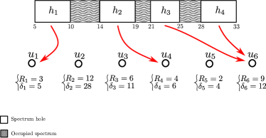
Figure 1: A depiction of an optimal solution to the tiny instance described in Example 1.

5 Computational Results

This section is devoted to evaluating the performance of the proposed B&P procedure against the best currently available ILP formulation of the problem, which is presented in [11], with respect to the CPU time. We implemented the B&P procedure in C++, and carried out the simulations on an Intel${}^{\text{\textregistered}}$ Core™ i7-9750H 2.60 GHz laptop with 16.00 GB of RAM, running Microsoft${}^{\text{\textregistered}}$ Windows${}^{\text{\textregistered}}$ 10 (64-bit) operating system. In our implementation of the B&P procedure, for solving the LP instances in the nodes of the search tree, we employed the IBM${}^{\text{\textregistered}}$ ILOG${}^{\text{\textregistered}}$ Concert CPLEX${}^{\text{\textregistered}}$ API.

As pointed out in the introduction, two 0-1 ILP formulations have been proposed in [11] for the problem. The (binary) integer linear programs obtained by using these formulations can be solved using the off-the-shelf ILP solvers like CPLEX and GUROBI. The second formulation, entitled “Linear Assignment Model (Type 2),” outperforms the first one, in terms of running time, and therefore, comparisons will be conducted against this formulation. Hereinafter we use the acronym LAM-T2 to refer to it. For the sake of self-containedness, we prsenet this formulation here. For every $j\in\{1,2,\ldots,N\}$ and every $i\in\{1,2,\ldots,M\}$, let the set $I_{j}(i)$ be defined by $I_{j}(i)=\{i^{\prime}\in\{i,i+1,\ldots,M\}\,|\,\beta_{i^{\prime}}-\alpha_{i}\leq\delta_{j}\}$. Moreover, for every $j\in\{1,2,\ldots,N\}$, let the set $T_{j}$ be defined as $T_{j}=\{i\in\{1,2,\ldots,M\}\,|\,\sum_{i^{\prime}\in I_{j}(i)}\mathrm{len}(h_{i^{\prime}})\geq R_{j}\}$. Finally, let the set $\Gamma$ be defined as $\Gamma=\{(j,i,i^{\prime})\,|\,j\in\{1,2,\ldots,N\},\,i\in T_{j},\,i^{\prime}\in I_{j}(i)\}$. Corresponding to each triple $(j,i,i^{\prime})\in\Gamma$, the formulation LAM-T2 contains a binary decision variable $\gamma^{j}_{ii^{\prime}}$. The formulation is as follows: l (LAM-T2) Maximize  ∑_j=1^N R_j ∑_i∈T_jγ^j_ii ,
subject to
∑_(j,i,i’)∈Γ γ_ii’^j≤1, for  i’=1,2,…,M,
∑_i∈T_j γ_ii^j≤1,  for j=1,2,…,N,
∑_i’∈I_j(i)len(h_i’)⋅γ^j_ii’≥R_j ⋅γ^j_ii , for  j= 1,2,…,N  and i∈T_j ,
γ_ii’^j∈{0,1}, for every (j,i,i’)∈Γ.

LAM-T2 consists of at most $NM^{2}$ binary decision variables and at most $M+N+NM$ linear constraints. In contrast to our formulation (BILP) which, due to its huge number of decision variables, cannot be fed directly to an ILP solver, the integer linear programs corresponding to LAM-T2, due to their compactness, can be solved by using an ILP solver. In our experiments, the CPLEX solver (Ver. 12.10.0.0) has been employed, both as an LP solver within the B&P routine and as an ILP solver for solving the integer linear programs corresponding to LAM-T2.

There are two remarks that should be made at this point. Firstly, the performance of the B&P search procedure can be improved by embedding a heuristic method for finding good integer-feasible solutions during the search process [23]. We didn’t employ such a heuristic method in the B&P process. However, by means of a powerful heuristic method for generating good integer-feasible solutions, the active nodes can more effectively be fathomed, which in turn makes the search process faster. Secondly, a decision has to be made as to which active node to visit first. Various node selection strategies have been described in the literature [23]. In our implementation of the B&P procedure, we employed the best-bound-first node selection rule. The unfathomed subproblems are maintained in a priority queue, and the one with the largest LP relaxation bound has the highest priority. For the case of two nodes with equal LP relaxation bounds, the one that is more likely to yield an integer-feasible solution is chosen.

To our knowledge, presently no benchmark dataset is available for the MC-HAP. We therefore created our own one, which contains more than 1000 randomly generated instances of the problem. The comparison has been made by the use of these instances. All the problem instances, and also their optimal solutions, are available online. As in [11], the TV band (470MHz – 862MHz) has been considered for the numerical simulations. In all the generated instances, the required bandwidth of a user is a random number (not necessarily integer) drawn uniformly from the range $[10,25]$ (in MHz). This is similar to that of [11], except that in our instances, the numbers are not necessarily integers. In the tables presented in this section, the parameter $q\in[0,1]$ determines the fraction of available spectrum in the frequency band, which is mainly determined by the geographical location. It has been shown that in urban areas, we have $q\approx 0.2$, whereas in suburban areas, $q\approx 0.8$ [11]. A time limit of 600 seconds has been set for each run. If the execution time for a run reaches this limit, the run halts and the best-so-far solution is reported.

A comparison of the average running times (in seconds) of B&P-SEP1 and B&P-SEP2 against those of the formulation LAM-T2, is tabulated in Table 2. The results (optimal objective values) of the three methods were entirely consistent with each other. For each row, we have considered 20 randomly generated instances of the problem. In the upper part of the table (first eight rows), as in [11, Table 1], for a user $u_{j}$, the parameter $\delta_{j}$ is drawn uniformly from the interval $[2R_{j},3R_{j}]$. Again, unlike the scenario described in [11], $\delta_{j}$s are not necessarily integers. In this part, $q$ is set to $0.5$. Moreover, the number of available holes for all the considered instances is equal to $25$, but for the number of users, we have $N\in\{25,50,\ldots,200\}$. In the lower part of the table (last six rows), we have $M=30$, $N\in\{30,60,\ldots,180\}$, and $q=0.25$. All $\delta_{j}$s are set equal to 45 $(1\leq j\leq N)$. As can be observed from the table, when the number of users is small, there is no major difference between the running times, but when the number of users is large, our approach has a much better performance.

Table 2: The effect of the ratio of the number of users to the number of holes on the time performance (in seconds) of the approaches. For each row, 20 random instances are used. The column labeled with “TL” reports the number of CPLEX runs stopped due to the time limit (for solving LAM-T2 models). None of the B&P-SEP1 and B&P-SEP2 runs reached the 600 seconds time limit.

$M$	$N$	$q$	$\delta$	B&P-SEP1	B&P-SEP2	LAM-T2	TL
25	25	0.5	As in [11, Table 1]	1.34	0.705	0.212	0
	50			1.30	0.670	0.795	0
	75			2.95	1.67	3.61	0
	100			1.22	1.06	12.0	0
	125			2.74	1.92	10.4	0
	150			2.22	1.70	47.7	1
	175			2.40	7.45	127	3
	200			3.04	3.58	162	4
30	30	0.25	45	1.50	0.525	0.240	0
	60			1.64	0.920	2.21	0
	90			1.01	1.14	4.26	0
	120			1.28	1.03	15.8	0
	150			0.910	0.730	6.30	0
	180			2.92	1.98	74.0	0

We empirically observed that when the ratio of the number of users to the number of holes is large, our method works much more effective than its counterpart LAM-T2. Table 3, in which a total of 600 instances of the problem are solved (60 instances per row), also provides a strong evidence for this fact. In this table, the parameter $\delta$ is set as in [11, Tables 1 and 2]. In the first five rows, we have $M\approx 30$, $N\in\{30,60,\ldots,150\}$, and $\delta_{j}\in[2R_{j},3R_{j}]$ ($1\leq j\leq N$). In the next five rows, we have $M\approx 50$, $N\in\{50,100,\ldots,250\}$, and $\delta_{j}\in[\max\{R_{j},15\},\min\{2R_{j},40\}]$ ($1\leq j\leq N$). For each row, 60 random instances are used.

Table 3: The effect of the ratio of the number of users to the number of holes on the time performance (in seconds) of the two approaches. For each row, 60 random instances are used. The column labeled with “TL” reports the number of CPLEX runs stopped due to the time limit (for solving LAM-T2 models). None of the B&P-SEP1 and B&P-SEP2 runs reached the 600 seconds time limit.

$M$	$N$	$\delta$	B&P-SEP1	B&P-SEP2	LAM-T2	TL
$\approx 30$	$30$	As in [11, Tab. 1]	1.17	2.67	0.293	0
	$60$		3.63	2.33	11.0	0
	$90$		3.98	1.49	32.2	2
	$120$		21.3	7.38	87.8	6
	$150$		32.7	11.8	90.8	8
$\approx 50$	$50$	As in [11, Tab. 2]	0.338	0.577	0.150	0
	$100$		0.773	0.493	1.04	0
	$150$		1.27	0.482	7.48	0
	$200$		0.802	0.715	27.8	1
	$250$		4.18	5.27	101	6

The superiority of the proposed B&P procedure stems from the strength (tightness) of the LP relaxation of the formulation (BILP). The LP relaxation of the formulation (BILP) can provide much tighter upper bounds than the LP relaxation of LAM-T2. To see this fact more clearly, we reported the optimal objective values of the LP relaxations of (BILP) and LAM-T2 for the 20 instances corresponding to the 8th row of Table 2, in which we have $M=25$, $N=200$, $q=0.5$, and $\delta_{j}\in[2R_{j},3R_{j}]$. Table 4 reports these values. The numbers in parentheses are the absolute integrality gaps. As can be seen, for a given instance, the LP relaxation of (BILP) can provide a much sharper upper-bound than the LP relaxation of LAM-T2. For example, for the 6th considered instance of the problem, the absolute integrality gap for (BILP) is 0.05, and for LAM-T2 is 24.435. These sharp upper-bounds allow for a much more effective pruning of the search tree, which is apparent in the performance of B&P-SEP1 and B&P-SEP2.

Table 4: The optimal objective values of the LP relaxations of (BILP) and LAM-T2 for the 20 instances corresponding to the 8th row of Table 2. For these instances, we have $M=25$, $N=200$, $q=0.5$, and $\delta_{j}\in[2R_{j},3R_{j}]$. The numbers in parentheses are the absolute integrality gaps.

	(BILP)	LAM-T2	Opt.		(BILP)	LAM-T2	Opt.
1	190.917 (0.117)	196.46 (5.66)	190.8	2	164.64 (0.04)	165.04 (0.44)	164.6
3	182.7 (0)	194.77 (12.07)	182.7	4	194.68 (0.08)	195.16 (0.56)	194.6
5	196.15 (0.05)	197.41 (1.31)	196.1	6	159.45 (0.05)	183.835 (24.435)	159.4
7	195.456 (0.056)	195.71 (0.31)	195.4	8	191.467 (0.067)	196.83 (5.43)	191.4
9	184.567 (0.067)	194.78 (10.28)	184.5	10	189.1 (0.1)	194.78 (5.78)	189
11	170.3 (0)	180.083 (9.783)	170.3	12	181.233 (0.33)	195.88 (14.68)	181.2
13	197.05 (0.05)	197.4 (0.4)	197	14	182.3 (0)	190.45 (8.15)	182.3
15	171.75 (0.05)	181.77 (10.07)	171.7	16	189.333 (0.033)	194.74 (5.44)	189.3
17	184.083 (0.083)	197.37 (13.37)	184	18	193.85 (0.05)	195.06 (1.26)	193.8
19	174.85 (0.05)	187.414 (12.614)	174.8	20	197.433 (0.033)	197.98 (0.58)	197.4

The parameter $\delta$ has a major impact on the behavior of LAM-T2. As has been stated in [11], as the value of $\delta$ grows, more variables and constraints need to be employed in LAM-T2, which increases the solution time. We observed that, as the value of $\delta$ increases, the execution time of our method increases as well. However, when the value of $\delta$ increases, our method shows a much better performance than its counterpart. In Table 5, we examine the effect of the value of $\delta$ on the performance of B&P-SEP1, B&P-SEP2, and LAM-T2. In this table, $\delta$ takes the values 30, 35, 40, and 45. In the first four rows, we have $M\approx 30$ and $N=120$, and in the next four rows $M\approx 30$ and $N=150$. For each row, 60 random instances are used. As can be observed from the table, as the value of $\delta$ increases, the performance difference becomes more pronounced. For example, for $M\approx 30$, $N=120$, and $\delta=45$, the average running time for B&P-SEP1 is 30, for B&P-SEP2 is 7.6, and for LAM-T2 is 302. Moreover, for 25 of the 60 runs corresponding to this row, CPLEX reached the time limit of 600 seconds when solving LAM-T2, and returned a feasible, and not necessarily optimal, solution.

Table 5: The effect of the value of $\delta$ on the time performance (in seconds) of the two approaches. For each row, 60 random instances are used. The column labeled with “TL” reports the number of CPLEX runs stopped due to the time limit (for solving LAM-T2 models). None of the B&P-SEP1 and B&P-SEP2 runs reached the 600 seconds time limit.

$M$	$N$	$\delta$	B&P-SEP1	B&P-SEP2	LAM-T2	TL
$\approx 30$	120	30	1.08	0.380	1.62	0
		35	2.43	2.60	27.2	2
		40	9.77	3.13	110	7
		45	30	7.60	302	25
$\approx 30$	150	30	1.64	0.972	1.34	0
		35	6.03	1.78	20.2	0
		40	15.6	9.03	111	9
		45	21.5	8.23	210	18

The integer-feasible but not necessarily optimal solutions that can be obtained during the B&B process are also valuable. When solving an instance of the ILP problem, sometimes we are satisfied with a solution that is integer-feasible, but not necessarily optimal. In these cases, we can set a time-limit for the solver. We are satisfied with the best solution that the solver has encountered during this period. This practice is more common for large instances for which obtaining the optimal solution may be very time consuming. Table 6 shows the B&P-SEP1 and B&P-SEP2 can obtain better feasible solutions than LAM-T2. In this table, only 90 seconds of time is given to the routines, and the best solution obtained is reported. In this table, we have considered 20 instances of the problem. For these instances, we have $M=70$, $N=70$, $q=0.25$, and $\delta_{j}\in[2R_{j},3R_{j}]$. As can be seen, the solutions obtained by B&P-SEP1 and B&P-SEP2 are of better quality than the solutions of LAM-T2.

We conclude this section by a brief comparison between the performance of B&P-SEP1 and B&P-SEP2. As can be observed from the Tables 2–6, both of these B&P procedures can provide a much better performance than LAM-T2. Generally, B&P-SEP2 performs better than B&P-SEP1. As can be seen from Table 6, the performance of the two routines in finding a good feasible solution as soon as possible was almost the same. However, we observed that, for some of the problem instances, B&P-SEP2 performed much better at proving the optimality. In fact, for B&P-SEP2, lowering the upper bound—so that it can be confirmed that the current incumbent is in fact optimal—was much better during the B&P process, for some of the considered problem instances. This can be regarded as the reason for its better performance.

Table 6: A comparison of the capability of the approaches to find feasible, and not necessarily optimal, solutions in 90 seconds. 20 instances of the problem have been considered. For these instances, we have $M=70$, $N=70$, $q=0.25$, and $\delta_{j}\in[2R_{j},3R_{j}]$.

	B&P-SEP1	B&P-SEP2	LAM-T2	Opt.		B&P-SEP1	B&P-SEP2	LAM-T2	Opt.
1	71.5	71.5	71.5	71.5	2	73.6	73.6	70.2	73.6
3	72.1	72.1	69.5	72.1	4	71.6	71.7	70.6	71.7
5	69.7	69.7	69.7	69.7	6	69.9	69.9	67.9	69.9
7	75.4	75.4	75.4	75.4	8	72.5	69.2	67.1	72.6
9	74.4	72.4	74.4	74.4	10	62.8	62.8	62.6	62.8
11	71.8	71.7	70.4	71.9	12	70.1	70.1	67.7	70.1
13	75.4	75.4	74.9	75.4	14	75.5	75.5	74.5	75.5
15	70.5	70.7	69.7	70.7	16	67.2	61.9	65.5	67.2
17	71.9	71.8	71	72.9	18	74.7	74.8	66.3	74.8
19	72.4	70.3	72.1	72.4	20	72.3	72.3	70.4	72.3

6 Conclusions

In this paper, we revisited the problem of spectrum hole assignment to cognitive secondary users with different hardware limitations. A novel 0-1 ILP formulation has been proposed, which provides very tight LP relaxation bounds. Moreover, we devised two different B&P procedures to overcome the problem of huge number of decision variables in the proposed formulation. Exhaustive numerical experiments demonstrate that the proposed approach can achieve a much better performance than the best currently available ILP formulation of the problem. Specifically, we reported some scenarios in which, the proposed approach was able to solve the problem instances in about 0.02 of the time required by its counterpart.

The work presented in this paper may be extended in different directions. Other user-specific parameters, rather than the MAR and the required bandwidth, may be taken into account in the problem formulation. For instance, the users may have different preferences about the spectrum holes, based on how much data-rate they can gain from each hole (due to their locations and/or technologies). Another direction is to take into consideration other metrics (objective functions) such as fairness, instead of considering only the spectrum utilization. Finally, incorporating learning mechanisms to predict the behavior of the PUs is a promising direction for future works. Based on analyzing the behavior of PUs, especially in scenarios where they may frequently change their spectrum usage pattern, we can seek for a more stable assignment. We may first rank the holes based on their availability probabilities, and then provide an acceptable hole assignment from the view point of stability.

7 Acknowledgements

This work was supported by by Iran’s National Elites Foundation (INEF).

References

- [1] D. Cabric, S. M. Mishra, R. W. Brodersen, Implementation issues in spectrum sensing for cognitive radios, in: Conference Record of the Thirty-Eighth Asilomar Conference on Signals, Systems and Computers, Vol. 1, 2004, pp. 772–776.
- [2] R. I. C. Chiang, G. B. Rowe, K. W. Sowerby, A quantitative analysis of spectral occupancy measurements for cognitive radio, in: IEEE 65th Vehicular Technology Conference - VTC2007 - Spring, 2007, pp. 3016–3020.
- [3] Federal Communications Commission (FCC), Spectrum policy task force – report of the spectrum efficiency working group, https://transition.fcc.gov/sptf/files/SEWGFinalReport_1.pdf (Nov. 2002).
- [4] The Office of Communications, Digital dividend : cognitive access – statement on licence-exempting cognitive devices using interleaved spectrum, https://www.ofcom.org.uk/__data/assets/pdf_file/0023/40838/statement.pdf (July 2009).
- [5] S. Haykin, Cognitive radio: brain-empowered wireless communications, IEEE J. Sel. Areas Commun. 23 (2) (2005) 201–220.
- [6] J. Mitola, G. Q. Maguire, Cognitive radio: making software radios more personal, IEEE Personal Communications 6 (4) (1999) 13–18.
- [7] Q. Zhao, B. M. Sadler, A survey of dynamic spectrum access, IEEE Signal Process. Mag. 24 (3) (2007) 79–89.
- [8] E. Z. Tragos, S. Zeadally, A. G. Fragkiadakis, V. A. Siris, Spectrum assignment in cognitive radio networks: A comprehensive survey, IEEE Commun. Surveys Tuts. 15 (3) (2013) 1108–1135.
- [9] F. Hu, B. Chen, K. Zhu, Full spectrum sharing in cognitive radio networks toward 5g: A survey, IEEE Access 6 (2018) 15754–15776.
- [10] A. Ahmad, S. Ahmad, M. H. Rehmani, N. U. Hassan, A survey on radio resource allocation in cognitive radio sensor networks, IEEE Commun. Surveys Tuts. 17 (2) (2015) 888–917.
- [11] J. Martinovic, E. Jorswieck, G. Scheithauer, A. Fischer, Integer linear programming formulations for cognitive radio resource allocation, IEEE Wireless Commun. Lett. 6 (4) (2017) 494–497.
- [12] J. Martinovic, E. Jorswieck, G. Scheithauer, The skiving stock problem and its application to cognitive radio networks, IFAC-PapersOnLine 49 (2016) 99–104.
- [13] Y. T. Hou, Y. Shi, H. D. Sherali, Spectrum sharing for multi-hop networking with cognitive radios, IEEE J. Sel. Areas Commun. 26 (1) (2008) 146–155.
- [14] P. Li, S. Guo, W. Zhuang, B. Ye, On efficient resource allocation for cognitive and cooperative communications, IEEE J. Sel. Areas Commun. 32 (2) (2014) 264–273.
- [15] D.-S. Chen, R. G. Batson, Y. Dang, Applied Integer Programming: Modeling and Solution, John Wiley & Sons, Ltd, Hoboken, NJ, 2011.
- [16] J. Desrosiers, M. E. Lübbecke, A primer in column generation, in: G. Desaulniers, J. Desrosiers, M. M. Solomon (Eds.), Column Generation, Springer US, Boston, MA, 2005, pp. 1–32.
- [17] F. Vanderbeck, Branching in branch-and-price: a generic scheme, Mathematical Programming 130 (2011) 249–294.
- [18] M. Dell’Amico, F. Furini, M. Iori, A branch-and-price algorithm for the temporal bin packing problem, Computers & Operations Research 114 (2020) 104825.
- [19] T. Öncan, A survey of the generalized assignment problem and its applications, INFOR: Information Systems and Operational Research 45 (3) (2007) 123–141.
- [20] M. Savelsbergh, A branch-and-price algorithm for the generalized assignment problem, Operations Research 45 (6) (1997) 831–841.
- [21] S. Elhedhli, L. Li, M. Gzara, J. Naoum-Sawaya, A branch-and-price algorithm for the bin packing problem with conflicts, INFORMS Journal on Computing 23 (3) (2011) 404–415.
- [22] R. Sadykov, F. Vanderbeck, Bin packing with conflicts: A generic branch-and-price algorithm, INFORMS Journal on Computing 25 (2) (2013) 244–255.
- [23] E. K. Lee, J. E. Mitchell, Integer programming: Branch and bound methods, in: C. A. Floudas, P. M. Pardalos (Eds.), Encyclopedia of Optimization, Springer US, Boston, MA, 2009, pp. 1634–1643.
- [24] J. M. Valério de Carvalho, Using extra dual cuts to accelerate column generation, INFORMS Journal on Computing 17 (2) (2005) 175–182.
- [25] F. Furini, E. Malaguti, A. Santini, An exact algorithm for the partition coloring problem, Computers & Operations Research 92 (2018) 170 – 181.
- [26] T. H. Cormen, C. E. Leiserson, R. L. Rivest, C. Stein, Introduction to Algorithms, 3rd Edition, The MIT Press, 2009.
- [27] H. Kellerer, U. Pferschy, D. Pisinger, Knapsack Problems, Springer-Verlag Berlin Heidelberg, 2004.