Run Time Analysis for Random Local Search
on Generalized Majority Functions

Abstract

Run time analysis of evolutionary algorithms recently makes significant progress in linking algorithm performance to algorithm parameters. However, settings that study the impact of problem parameters are rare. The recently proposed W-model provides a good framework for such analyses, generating pseudo-Boolean optimization problems with tunable properties.

We initiate theoretical research of the W-model by studying how one of its properties—neutrality—influences the run time of random local search. Neutrality creates plateaus in the search space by first performing a majority vote for subsets of the solution candidate and then evaluating the smaller-dimensional string via a low-level fitness function.

We prove upper bounds for the expected run time of random local search on this Majority problem for its entire parameter spectrum. To this end, we provide a theorem, applicable to many optimization algorithms, that links the run time of Majority with its symmetric version HasMajority, where a sufficient majority is needed to optimize the subset. We also introduce a generalized version of classic drift theorems as well as a generalized version of Wald’s equation, both of which we believe to be of independent interest.

I Introduction

Randomized search heuristics, such as evolutionary algorithms (EAs), have been applied with great success to real-world optimization problems for which the user is faced with limited information about the problem or limited resources to solve it. This is an impressive feat, since such problems are typically hard due to a combination of different challenging features. In order to better understand the reasons behind why EAs perform so well in such settings, theoretical results analyze benchmark functions that encapsulate specific features assumed to be also present in real-world problems. At present, these functions are typically unrelated to each other, and it is difficult to derive how they interact with one another. This makes it hard to translate such theoretical results to more realistic problems. An alternative approach for deriving theoretical results is to consider a class of different functions that can be combined in well-defined ways, allowing to provide guarantees for more complex problems. The recently introduced W-model [1] provides such function classes. Given a pseudo-Boolean function $f$, the W-model proposes a sequence of four independent steps that each change a different feature of $f$. The degree by which each feature is changed is regulated by parameters specific to each step. Thus, overall, the W-model allows to create a diverse set of functions, all based on $f$, that showcases various features in different intensities.

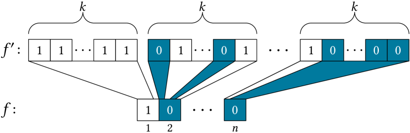
Figure 1: Given a pseudo-Boolean function $f$ defined over bit strings of length $n\in\mathds{N}_{>0}$ and a parameter $k\in\mathds{N}_{>0}$, neutrality creates a function $f^{\prime}$ defined over bit strings of length $nk$, consisting of $n$ blocks of length $k$ each. When evaluating $f^{\prime}$, first, for each of the $k$ blocks, the majority of its bits is determined. Then, $f$ is evaluated on the resulting bit string of length $n$ of the majority outcomes.

In this article, we initiate the run time analysis of the W-model. To this end, we focus on one of its features called neutrality. Given a function $f$ defined over bit strings of length $n$ as well as an integer parameter $k$, neutrality substitutes each bit of a length-$n$ bit string by $k$ bits. When evaluating a new bit string of length $nk$, each of the subsequent blocks of $k$ bits is reduced to the majority among its bit values, and the resulting bit string of length $n$ is evaluated by $f$ (see Figure 1). Overall, neutrality introduces a two-stage process into the optimization of $f$. On a high level, $f$ is optimized. On a low level, the correct majority value of each block is determined. Assuming that the different blocks are independent, analyzing the run times of the two stages separately and then combining these results leads to a run time result for $f$.

Doerr et al. [2] analyzed the high-level approach of the aforementioned two-stage process diligently for the class of separable functions, where a function is separable if its value is the sum of the values of $n$ independent sub-functions. The authors show that the run time of random local search (RLS) and of the $(1+1)~{}\textrm{EA}$ is, in expectation, bounded from above by the slowest expected run time of a sub-function times $\ln(n)$. The logarithmic overhead is a result of the classical coupon collector problem that accounts for optimizing all $n$ sub-functions correctly.

The second stage of the two-stage optimization process sketched above concerns analyzing the run time of a majority function. Since the value returned by such a function only changes if the majority of the bits in its input changes, this leads to analyzing the behavior of an algorithm in a landscape of equal fitness, called a plateau. Changing the number of bits to the optimal majority requires an EA to perform a random walk on the plateau until finding the optimal majority, at which point in time the block is optimized. We refer to this search behavior as crossing the plateau.

In order to better understand the impact of the plateau size on the optimization process, we extend the notion of majority for the W-model. To this end, we introduce the function $\textsc{HasMajority}_{r}$, defined over bit strings of length $n\in\mathds{N}^{+}$ (where $n$ is even), having a parameter $r\in[0,n/2]\cap\mathds{N}$ how strong the majority has to be in order to be counted. $\textsc{HasMajority}_{r}$ takes the two values $0$ and $1$. A bit string has a $\textsc{HasMajority}_{r}$-value of $1$ if its number of $0$s or its number of $1$s is at least $n/2+r$, and it has a value of $0$ otherwise. We also introduce the asymmetric version $\textsc{Majority}_{r}$, where a bit string only has a function value of $1$ if it has at least $n/2+r$ $1$s (and it is $0$ otherwise).

Our results

We analyze RLS, which iteratively constructs new solutions by flipping exactly one bit, chosen uniformly at random, in its currently best solution. We bound the expected run time of RLS, that is, the number of iterations until an optimal solution is found for the first time, on HasMajority and Majority from above for the entire range of $r$. Using the results by Doerr et al. [2], this implies run time bounds for OneMax with added neutrality (Corollary 13). We first analyze the symmetric case of HasMajority (similar to the result by Bian et al. [3]) and show with Theorem 6 the complex dependency of the run time of RLS on the parameter $r$, resulting in multiple different regimes (Figure 2). For values of $r$ constant in $n$, the run time is constant, and it grows quadratically in $r$ until $r=\mathrm{O}\mathopen{}\mathclose{{}\left({\sqrt{n}}}\right)$. For $r=\omega\mathopen{}\mathclose{{}\left({\sqrt{n}}}\right)\cap\mathrm{o}\mathopen{}\mathclose{{}\left({n}}\right)$, the expected run time is mainly given by an exponential in $r^{2}/n$. For the remaining regime of $r$, the expected run time is at least exponential. The behavior for Majority is similar, as Theorem 7 shows. The main difference is an overhead of $n\ln(r)$, which is caused by the larger size of the plateau. For the special case $r=n/2-1$, the Majority function reduces to the well-known Needle function, for which the run time of RLS, the $(1+1)~{}\textrm{EA}$ (EA), and a number of generalizations are very well understood [4, 5].

Our result for Majority is based on a restart argument applied to HasMajority. Since such restart arguments are not specific to the context of EAs or even optimization, we analyze the situation in a general setting (Theorem 8). Our result applies to any assortment of interleaved stopping times. We prove Theorem 8 via a generalized version of Wald’s equation (Theorem 5), which we could not find in this detail and generality in the literature. We prove the generalized version of Wald’s equation via a new general basic drift theorem (Theorem 4), which relates the expected progress of a random process more explicitly to the values at the start and at the end of the process than traditional drift theorems. As all of these theorems relate to scenarios commonly found in the analysis of EAs, we are confident that they are of independent interest.

With Corollary 9, we explicitly connect the expected run times of HasMajority and Majority for a large class of EAs, providing a general framework for our setting. This result comes with multiple conditions, due to its generality. However, we also provide additional statements (Lemmas 10 and 11) that show that many EAs satisfy the conditions of Corollary 9. In order to apply Corollary 9 to any EA we cover with this framework, it then remains to provide bounds on the expected run time of an EA on HasMajority. We note that this framework is also useful in the setting of deletion-robust optimization, as studied by Bian et al. [3], since Majority occurs as a subproblem there.

We complement our theoretical analyses with empirical investigations of the RLS variant RLS_ℓ, which flips exactly $\ell\in[1,n]\cap\mathds{N}$ bits (chosen uniformly among all $\ell$-cardinality subsets), on Majority. For $r=\lfloor\sqrt{n}\rfloor$, we consider the empirical run time for different values of $\ell$, and we find that a value around $n/2$ leads to the lowest run time (Figure 5), which is by orders of magnitude lower than the empirical run time of conventional RLS. Additional results, which look into the trajectory of the best solution so far over time, reveal that while instantiations of RLS_ℓ for different values of $\ell$ have qualitatively the same random-walk behavior, the larger step size for larger values of $\ell$ makes it easier to find a global optimum (Figure 6). However, we note that there is a limit to how many bits to flip during a single iteration makes sense, as, for example, inverting the bit string in each iteration makes RLS_n alternate between just two solutions. Nonetheless, a high mutation rate in the order of $n$ seems beneficial for our setting.

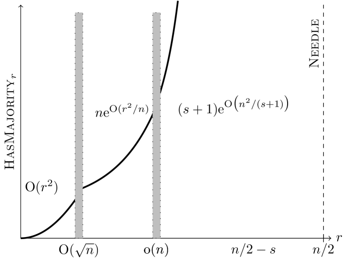
Figure 2: The dependency of the expected run time of RLS on $\textsc{HasMajority}_{r}$ with respect to the majority parameter $r$ as proven in Theorem 6. The gray boxes denote regions in which the asymptotics switch (sharply) from $\mathrm{O}\mathopen{}\mathclose{{}\left({\sqrt{n}}}\right)$ to $\omega\mathopen{}\mathclose{{}\left({\sqrt{n}}}\right)$ and from $\mathrm{o}\mathopen{}\mathclose{{}\left({n}}\right)$ to $\Theta\mathopen{}\mathclose{{}\left({n}}\right)$. The value $s\in\mathds{N}$ is any value such that there is a $c\in\Theta\mathopen{}\mathclose{{}\left({1}}\right)$ with $c<1/2$ such that $s\leq cn$. The dashed line at $n/2$ denotes the run time on Needle.

Related work

Analyzing the performance of EAs on plateaus by theoretical means is a well-established concept. The arguably most studied benchmark function with a plateau is Jump, existing in different variants, many of which were proposed recently [5, 6, 7, 8]. However, the problem posed by the plateau in Jump is typically different than from crossing a plateau, as we discuss in the following. In its classical variant, Jump consists of a slope toward the unique global optimum, which itself is surrounded by solutions with worse function values (called the valley). The plateau is the set of points with second-best function value. For Jump, the behavior of an EA on the plateau is typically not that important, but rather that the valley is overcome, oftentimes referred to as jumping over the valley. This is in contrast to crossing a plateau, where the behavior of an EA on the plateau is very important. The main importance of jumping remains true for Jump when shifting the global optimum [7] and/or increasing the number of global optima to jump to [6, 8]. However, the picture changes when considering EAs that apply crossover, that is, combining different solutions when creating new ones. Then, the random walk on the plateau becomes relevant for the expected run time on Jump [9, 10, 11]. Nonetheless, in such a setting, it is primarily important to create diverse solutions on the plateau, in order to leave it via crossover, instead of crossing the plateau (by finding a better solution next to it).

One variant of Jump, recently introduced by Antipov and Doerr [5], which removes the valley and increases the plateau, actually requires dealing with crossing the plateau. The authors analyze the $(1+1)~{}\textrm{EA}$ on this variant and determine an exact run time bound (up to lower-order terms) via arguments on Markov chains. In contrast to our setting, where the set of global optima is typically very large (in the order of $\binom{n}{n/2+r}$), their function has a unique global optimum.

In another recent paper, Bian et al. [3] analyzed the $(1+1)~{}\textrm{EA}$ on Majority as a side result when considering deletion-robust linear optimization. Using our notion of Majority, their result holds for values of $r=\mathrm{O}\mathopen{}\mathclose{{}\left({\sqrt{n\log n}}}\right)$, that is, not for the entire range of $r$ up to $n/2$. Further, their result does not seem to be tight, as for values of $r=\Theta\mathopen{}\mathclose{{}\left({1}}\right)$, their bound is $\mathrm{O}\mathopen{}\mathclose{{}\left({n^{2}}}\right)$, whereas we show a constant bound, albeit for RLS.

Outline

In Section II, we introduce our notation, formalize our problem, and provide the mathematical tools we use for our analysis. Especially, we prove Theorems 4 and 5, which we believe are of independent interest. In Section III, we analyze RLS on HasMajority (Theorem 6) and Majority (Theorem 7). Further, we provide the theorem for decomposing stopping times (Theorem 8), show how it can be used to relate the expected run times of EAs on HasMajority and Majority (Corollary 9), and put everything together to prove our main result, the run time bound for RLS optimizing OneMax with added neutrality from the W-model (Corollary 13). Section IV describes our empirical results. Last, we conclude with Section V and suggest ideas for future work.

II Preliminaries

Let $\mathds{N}$ denote the set of natural numbers, including $0$. For all $m,n\in\mathds{N}$, let $[m..n]\coloneqq[m,n]\cap\mathds{N}$, and let $[m]\coloneqq[1..m]$. Further, let $\mathds{R}$ denote the set of reals, and let $\overline{\mathds{R}}=\mathds{R}\cup\{-\infty,\infty\}$. For the sake of conciser notations, we define that $\infty\cdot 0=0=-\infty\cdot 0$. We say that a random variable $X$ over $\mathds{R}$ is integrable if and only if $\mathrm{E}\mathopen{}\mathclose{{}\left[{|X|}}\right]<\infty$. Note that integrability of $X$ implies that $X$ is almost surely finite. We extend this concept to random processes and say that $(X_{t})_{t\in\mathds{N}}$ is integrable if and only if for each $t\in\mathds{N}$, it holds that $X_{t}$ is integrable.

Let $n\in\mathds{N}_{>0}$. We call each $\bm{x}\in\{0,1\}^{n}$ an individual and its components bits. Further, for all $b\in\{0,1\}$, let $|\bm{x}|_{b}\coloneqq|\{i\in[n]\mid\bm{x}_{i}=b\}|$. We call any real-valued function over individuals a fitness function.

Let $n\in\mathds{N}_{>0}$ be even, and let $r\in[0..n/2]$. We consider the two fitness functions $\textsc{HasMajority}_{r}$ and $\textsc{Majority}_{r}$, where, for all $\bm{x}\in\{0,1\}^{n}$, it holds that

$$\textsc{HasMajority}_{r}(\bm{x}) =\mathds{1}{(\max\{|\bm{x}|_{0},|\bm{x}|_{1}\}\geq n/2+r)}\textrm{ and}$$

$$\textsc{Majority}_{r}(\bm{x}) =\mathds{1}{(|\bm{x}|_{1}\geq n/2+r)},$$

where $\mathds{1}{(\mathcal{E})}$ is the indicator function that evaluates to $1$ if event $\mathcal{E}$ occurs and that evaluates to $0$ otherwise. When we drop the index $r$ and only mention HasMajority or Majority, we mean that the respective statement holds for all $r\in[0..n/2]$.

We note that HasMajority and Majority are special cases of the functions mentioned in Section I with the target string $\bm{z}\in\{0,1\}^{n}$ being the all-$1$s string. Since we only consider algorithms that treat $0$s and $1$s symmetrically, analyzing HasMajority and Majority as defined above covers without loss of generality the more general function class discussed in Section I.

We consider evolutionary algorithms (EAs) to be (possibly random) sequences $(\bm{x}^{(t)})_{t\in\mathds{N}}$ over $\{0,1\}^{n}$. Typically, the sequence of an EA $A$ depends (among others) on a fitness function $f$, and is not well-defined otherwise. We refer to well-defined sequences by saying that $A$ optimizes $f$.

A specific EA that we are interested in and that optimizes a fitness function is random local search (RLS, Algorithm 1). Note that for RLS to optimize $f$ and the respective sequence to be well-defined, in addition to $f$, an initialization distribution needs to be specified. Typically, the uniform distribution is chosen. However, since we require for some of our results that RLS starts at a specific position in the search space, we consider general initialization distributions.

Given an EA $(\bm{x}^{(t)})_{t\in\mathds{N}}$ optimizing a fitness function $f$, we call $\inf\{t\in\mathds{N}\mid f\big{(}\bm{x}^{(t)}\big{)}=\max\mathrm{rng}\mathopen{}\mathclose{{}\left({f}}\right)\}$ the run time of the algorithm on $f$. Note that the set that the infimum is taken over may be empty. To this end, we define $\inf\emptyset=\infty$. Further note that the run time can be a random variable. We refer to the expectation of the run time as the expected run time.

1 $\bm{x}^{(0)}\sim D$;

2 for $t\in\mathds{N}$ do

3       $\bm{y}\leftarrow$ flip exactly one bit in $\bm{x}^{(t)}$, chosen uniformly at random;

4       if $f(\bm{y})\geq f\big{(}\bm{x}^{(t)}\big{)}$ then $\bm{x}^{(t+1)}\leftarrow\bm{y}$;

5       else $\bm{x}^{(t+1)}\leftarrow\bm{x}^{(t)}$;

6      

Algorithm 1 Random local search (RLS) with initialization distribution $D$, maximizing $f\colon\{0,1\}^{n}\to\mathds{R}$.

II-A Tools

Besides basic tools from probability theory, we apply drift analysis [12]. Most prominently, we use the additive-drift theorem, originally introduced by He and Yao [13], as well as the multiplicative-drift theorem, originally introduced by Doerr et al. [14]. We state the theorems in a general fashion, as provided by Kötzing and Krejca [15], removing some unnecessary assumptions.

Theorem 1 (Additive drift, upper bound [15, Theorem $7$]).

Let $(X_{t})_{t\in\mathds{N}}$ be an integrable random processes over $\mathds{R}_{\geq 0}$, adapted to a filtration $(\mathcal{F}_{t})_{t\in\mathds{N}}$, and let $T$ be a stopping time with respect to $\mathcal{F}$. Assume that there is a $\delta\in\mathds{R}_{>0}$ such that, for all $t\in\mathds{N}$, it holds that

$$\big{(}X_{t}-\mathrm{E}\mathopen{}\mathclose{{}\left[{X_{t+1}\ \mathopen{}\mathclose{{}\left|\ \vphantom{X_{t+1}}\mathcal{F}_{t}}\right.}}\right]\big{)}\cdot\mathds{1}{(t<T)}\geq\delta\cdot\mathds{1}{(t<T)}.$$ (1)

Then $\mathrm{E}\mathopen{}\mathclose{{}\left[{T\ \mathopen{}\mathclose{{}\left|\ \vphantom{T}\mathcal{F}_{0}}\right.}}\right]\leq(X_{0}-\mathrm{E}\mathopen{}\mathclose{{}\left[{X_{T}\ \mathopen{}\mathclose{{}\left|\ \vphantom{X_{T}}\mathcal{F}_{0}}\right.}}\right])/\delta$.

Theorem 2 (Multiplicative drift, upper bound [15, Corollary $16$]).

Let $(X_{t})_{t\in\mathds{N}}$ be an integrable random processes over $\mathds{R}$, adapted to a filtration $(\mathcal{F}_{t})_{t\in\mathds{N}}$, with $X_{0}\geq 1$, and let $T=\inf\{t\in\mathds{N}\mid X_{t}<1\}$. Assume that there is a $\delta\in\mathds{R}_{>0}$ such that, for all $t\in\mathds{N}$, it holds that

$$\big{(}X_{t}-\mathrm{E}\mathopen{}\mathclose{{}\left[{X_{t+1}\ \mathopen{}\mathclose{{}\left|\ \vphantom{X_{t+1}}\mathcal{F}_{t}}\right.}}\right]\big{)}\cdot\mathds{1}{(t<T)}\geq\delta\cdot X_{t}\cdot\mathds{1}{(t<T)}.$$ (2)

Then $\mathrm{E}\mathopen{}\mathclose{{}\left[{T\ \mathopen{}\mathclose{{}\left|\ \vphantom{T}\mathcal{F}_{0}}\right.}}\right]\leq\big{(}1+\ln(X_{0})\big{)}/\delta$.

In addition to these theorems, we apply a general version of Wald’s equation (Theorem 5), which we prove using a new general drift theorem (Theorem 4), as we could not find a statement this general in the literature. We prove Theorem 4 by using the optional-stopping theorem (Theorem 3), similar to how Kötzing and Krejca [15] derived their results.

Theorem 3 (Optional stopping [16, Theorems $4.8.4$ and $4.8.5$], [17, Slide $12$]).

Let $S$ be a stopping time with respect to a filtration $\mathopen{}\mathclose{{}\left(\mathcal{F}_{i}}\right)_{i\in\mathds{N}}$, and let $\mathopen{}\mathclose{{}\left(X_{i}}\right)_{i\in\mathds{N}}$ be a random process over $\overline{\mathds{R}}$, adapted to $\mathcal{F}$.

1. If $X$ is a non-negative supermartingale, then $\mathrm{E}\mathopen{}\mathclose{{}\left[{X_{S}\ \mathopen{}\mathclose{{}\left|\ \vphantom{X_{S}}\mathcal{F}_{0}}\right.}}\right]\leq X_{0}$.

2. If $\mathrm{E}\mathopen{}\mathclose{{}\left[{S}}\right]<\infty$ and if $X$ is a submartingale such that there is a $c\in\mathds{R}$ such that, for all $i\in\mathds{N}$, it holds that $\mathrm{E}\mathopen{}\mathclose{{}\left[{|X_{i}-X_{i+1}|\ \mathopen{}\mathclose{{}\left|\ \vphantom{|X_{i}-X_{i+1}|}\mathcal{F}_{i}}\right.}}\right]\cdot\mathds{1}{(i<S)}\leq c$, then $\mathrm{E}\mathopen{}\mathclose{{}\left[{X_{S}\ \mathopen{}\mathclose{{}\left|\ \vphantom{X_{S}}\mathcal{F}_{0}}\right.}}\right]\geq X_{0}$.

The basic-drift theorem below is a generalization of the most commonly used drift theorems. However, in contrast to those, it relates the accumulated drift to the overall change in potential instead of explicitly solving for the first-hitting time. It is thus more akin to the (deterministic) potential method [18, Chapter $17.3$], extending it to random variables. This allows to estimate the accumulated cost of operations rather than only the amount of operations.

Theorem 4 (Basic drift).

Let $S$ be a stopping time with respect to a filtration $\mathopen{}\mathclose{{}\left(\mathcal{F}_{i}}\right)_{i\in\mathds{N}}$, and let $\mathopen{}\mathclose{{}\left(X_{i}}\right)_{i\in\mathds{N}}$ and $\mathopen{}\mathclose{{}\left(\delta_{i}}\right)_{i\in\mathds{N}}$ be random processes over $\overline{\mathds{R}}$ such that $(X_{i}\cdot\mathds{1}{(i\leq S)})_{i\in\mathds{N}}$ and $(\delta_{i}\cdot\mathds{1}{(i<S)})_{i\in\mathds{N}}$ are integrable and adapted to $\mathcal{F}$ ​​.

1. Assume that $(X_{i}\cdot\mathds{1}{(i\leq S)})_{i\in\mathds{N}}$ and $(\delta_{i}\cdot\mathds{1}{(i<S)})_{i\in\mathds{N}}$ are non-negative and that for all $i\in\mathds{N}$, it holds that

   $$\Big{(}X_{i}-\mathrm{E}\big{[}{X_{i+1}\ \big{|}\ \vphantom{X_{i+1}}\mathcal{F}_{i}}\big{]}\Big{)}\cdot\mathds{1}{(i<S)}\geq\delta_{i}\cdot\mathds{1}{(i<S)}.$$ (DC-u)

   Then

   $$\mathrm{E}\mathopen{}\mathclose{{}\left[{\sum\nolimits_{i\in[S]}\delta_{i-1}\ \mathopen{}\mathclose{{}\left|\ \vphantom{\sum\nolimits_{i\in[S]}\delta_{i-1}}\mathcal{F}_{0}}\right.}}\right]\leq X_{0}-\mathrm{E}\big{[}{X_{S}\ \big{|}\ \vphantom{X_{S}}\mathcal{F}_{0}}\big{]}.$$ (3)

2. Assume that $\mathrm{E}\mathopen{}\mathclose{{}\left[{S}}\right]<\infty$, and that there is a $c\in\mathds{R}$ such that for all $i\in\mathds{N}$, it holds that $\mathrm{E}\mathopen{}\mathclose{{}\left[{|X_{i}-X_{i+1}-\delta_{i}|\ \mathopen{}\mathclose{{}\left|\ \vphantom{|X_{i}-X_{i+1}-\delta_{i}|}\mathcal{F}_{i}}\right.}}\right]\cdot\mathds{1}{(i<S)}\leq c$, and that for all $i\in\mathds{N}$, it holds that

   $$\Big{(}X_{i}-\mathrm{E}\big{[}{X_{i+1}\ \big{|}\ \vphantom{X_{i+1}}\mathcal{F}_{i}}\big{]}\Big{)}\cdot\mathds{1}{(i<S)}\leq\delta_{i}\cdot\mathds{1}{(i<S)}.$$ (DC-l)

   Then

   $$\mathrm{E}\mathopen{}\mathclose{{}\left[{\sum\nolimits_{i\in[S]}\delta_{i-1}\ \mathopen{}\mathclose{{}\left|\ \vphantom{\sum\nolimits_{i\in[S]}\delta_{i-1}}\mathcal{F}_{0}}\right.}}\right]\geq X_{0}-\mathrm{E}\big{[}{X_{S}\ \big{|}\ \vphantom{X_{S}}\mathcal{F}_{0}}\big{]}.$$

Proof.

Let $\mathopen{}\mathclose{{}\left(Z_{i}}\right)_{i\in\mathds{N}}$ be such that for all $i\in\mathds{N}$, it holds that $Z_{i}=X_{i}+\sum\nolimits_{k\in[i]}\delta_{k-1}$. We aim to apply Theorem 3 to the stopped process $\mathopen{}\mathclose{{}\left(Y_{i}}\right)_{i\in\mathds{N}}$ of $Z$, and to $S$ and $\mathcal{F}$. To this end, for all $i\in\mathds{N}$, let

$$Y_{i}=Z_{i}\cdot\mathds{1}{(i\leq S)}+Z_{S}\cdot\mathds{1}{(i>S)}.$$

Note that, all by assumption, $S$ is a stopping time with respect to $\mathcal{F}$, and $Y$ is integrable and adapted to $\mathcal{F}$, due to $(X_{i}\cdot\mathds{1}{(i\leq S)})_{i\in\mathds{N}}$ and $(\delta_{i}\cdot\mathds{1}{(i<S)})_{i\in\mathds{N}}$ having these properties.

We are left to show that $Y$ is a super- or a submartingale with additional properties. To this end, we first consider the expected change of $Y$. Let $i\in\mathds{N}$. Noting that $S$ is integer, observe that

$$Y_{i}-\mathrm{E}\mathopen{}\mathclose{{}\left[{Y_{i+1}\ \mathopen{}\mathclose{{}\left|\ \vphantom{Y_{i+1}}\mathcal{F}_{i}}\right.}}\right]$$

$$\quad=Z_{i}\cdot\overbrace{\mathds{1}{(i\leq S)}}^{\mathclap{=\mathds{1}{(i=S)}+\mathds{1}{(i<S)}}}+Z_{S}\cdot\mathds{1}{(i>S)}$$

$$\qquad-\mathrm{E}\big{[}{Z_{i+1}\cdot\overbrace{\mathds{1}{(i+1\leq S)}}^{\mathclap{=\mathds{1}{(i<S)}}}+Z_{S}\cdot\mathds{1}{(i+1>S)}\ \big{|}\ \vphantom{Z_{i+1}\cdot\overbrace{\mathds{1}{(i+1\leq S)}}^{\mathclap{=\mathds{1}{(i<S)}}}+Z_{S}\cdot\mathds{1}{(i+1>S)}}\mathcal{F}_{i}}\big{]}$$

$$\quad=\big{(}Z_{i}-\mathrm{E}\mathopen{}\mathclose{{}\left[{Z_{i+1}\ \mathopen{}\mathclose{{}\left|\ \vphantom{Z_{i+1}}\mathcal{F}_{i}}\right.}}\right]\big{)}\cdot\mathds{1}{(i<S)}+Z_{i}\cdot\mathds{1}{(i=S)}$$

$$\qquad+Z_{S}\cdot\mathrm{E}\big{[}{\overbrace{\mathds{1}{(i>S)}-\mathds{1}{(i+1>S)}}^{=-\mathds{1}{(i=S)}}\ \big{|}\ \vphantom{\overbrace{\mathds{1}{(i>S)}-\mathds{1}{(i+1>S)}}^{=-\mathds{1}{(i=S)}}}\mathcal{F}_{i}}\big{]}$$

$$\quad=\big{(}Z_{i}-\mathrm{E}\mathopen{}\mathclose{{}\left[{Z_{i+1}\ \mathopen{}\mathclose{{}\left|\ \vphantom{Z_{i+1}}\mathcal{F}_{i}}\right.}}\right]\big{)}\cdot\mathds{1}{(i<S)}$$

$$\quad=\big{(}X_{i}-\mathrm{E}\mathopen{}\mathclose{{}\left[{X_{i+1}\ \mathopen{}\mathclose{{}\left|\ \vphantom{X_{i+1}}\mathcal{F}_{i}}\right.}}\right]-\delta_{i}\big{)}\cdot\mathds{1}{(i<S)}.$$ (4)

Whether $Y$ is a super- or a submartingale is determined by the sign of eq. 4, noting that $\mathds{1}{(i<S)}\geq 0$. To this end, we consider the two cases of Theorem 4 separately.

Item a). By eq. DC-u, it follows that eq. 4 is greater or equal to zero. Thus, $Y$ is a supermartingale. Further, due to the assumptions of Theorem 4 item a), $Y$ is non-negative. Applying Theorem 3 item a), by the linearity of expectation and noting that $S\geq 0$, we get

$$\mathrm{E}\mathopen{}\mathclose{{}\left[{X_{S}\ \mathopen{}\mathclose{{}\left|\ \vphantom{X_{S}}\mathcal{F}_{0}}\right.}}\right]+\mathrm{E}\mathopen{}\mathclose{{}\left[{\sum\nolimits_{i\in[S]}\delta_{i-1}\ \mathopen{}\mathclose{{}\left|\ \vphantom{\sum\nolimits_{i\in[S]}\delta_{i-1}}\mathcal{F}_{0}}\right.}}\right] =\mathrm{E}\mathopen{}\mathclose{{}\left[{Y_{S}\ \mathopen{}\mathclose{{}\left|\ \vphantom{Y_{S}}\mathcal{F}_{0}}\right.}}\right]$$ (5)

$$\leq Y_{0}=X_{0}.$$

Subtracting by $\mathrm{E}\mathopen{}\mathclose{{}\left[{X_{S}\ \mathopen{}\mathclose{{}\left|\ \vphantom{X_{S}}\mathcal{F}_{0}}\right.}}\right]$ proves this case.

Item b). Similar to the previous case, by eq. DC-l, it follows that eq. 4 is less or equal to zero. Thus, $Y$ is a submartingale. By the assumptions of Theorem 4 item b), it follows that $Y$ has uniformly bounded expected differences. Recalling that, by assumption, $\mathrm{E}\mathopen{}\mathclose{{}\left[{S}}\right]<\infty$ in this case and by applying Theorem 3 item b), the same result as in eq. 5 follows but with the inequality sign flipped, concluding this case and thus the proof. ∎

An application of Theorem 4 is the generalization of Wald’s equation below. In contrast to more common statements of Wald’s equation, this version neither assumes that the individual summands follow the same law nor that they are independent. In the context of run time analysis, it is useful when aiming to split the run time into phases. Instead of having to calculate the entire expected run time all at once, the theorem states that it is sufficient to calculate the expected run time of each phase (and then add them). The latter is typically far easier, especially since the theorem allows to choose a filtration. This result was recently applied in the analysis of infection processes, where it was used in order to translate statements about discrete time to continuous time [19].

Theorem 5 (Generalized Wald’s equation).

Let $S$ be an integrable stopping time with respect to a filtration $\mathopen{}\mathclose{{}\left(\mathcal{F}_{i}}\right)_{i\in\mathds{N}}$. Further, let $\mathopen{}\mathclose{{}\left(X_{i}}\right)_{i\in\mathds{N}_{>0}}$ be a random process over $\overline{\mathds{R}}_{\geq 0}$ such that $\sum_{i\in[S]}X_{i}$ is integrable and such that there exists a $c\in\mathds{R}$ such that for all $i\in\mathds{N}$, it holds that $\mathrm{E}\mathopen{}\mathclose{{}\left[{\big{|}X_{i+1}-\mathrm{E}\mathopen{}\mathclose{{}\left[{X_{i+1}\ \mathopen{}\mathclose{{}\left|\ \vphantom{X_{i+1}}\mathcal{F}_{i}}\right.}}\right]\big{|}\ \mathopen{}\mathclose{{}\left|\ \vphantom{\big{|}X_{i+1}-\mathrm{E}\mathopen{}\mathclose{{}\left[{X_{i+1}\ \mathopen{}\mathclose{{}\left|\ \vphantom{X_{i+1}}\mathcal{F}_{i}}\right.}}\right]\big{|}}\mathcal{F}_{i}}\right.}}\right]\cdot\mathds{1}{(i<S)}\leq c$. Then $\mathrm{E}\mathopen{}\mathclose{{}\left[{\sum_{i\in[S]}X_{i}\ \mathopen{}\mathclose{{}\left|\ \vphantom{\sum_{i\in[S]}X_{i}}\mathcal{F}_{0}}\right.}}\right]=\mathrm{E}\mathopen{}\mathclose{{}\left[{\sum_{i\in[S]}\mathrm{E}\mathopen{}\mathclose{{}\left[{X_{i}\ \mathopen{}\mathclose{{}\left|\ \vphantom{X_{i}}\mathcal{F}_{i-1}}\right.}}\right]\ \mathopen{}\mathclose{{}\left|\ \vphantom{\sum_{i\in[S]}\mathrm{E}\mathopen{}\mathclose{{}\left[{X_{i}\ \mathopen{}\mathclose{{}\left|\ \vphantom{X_{i}}\mathcal{F}_{i-1}}\right.}}\right]missing}\mathcal{F}_{0}}\right.}}\right]$.

Checking that $\sum_{i\in[S]}X_{i}$ is integrable can prove challenging in certain cases. However, if this sum can be expressed as a single stopping time, Theorem 4 item a) might be used to show that the sum is integrable.

Proof of Theorem 5.

Let $\mathopen{}\mathclose{{}\left(Y_{i}}\right)_{i\in\mathds{N}}$ be such that for all $i\in\mathds{N}$, it holds that $Y_{i}=\mathrm{E}\mathopen{}\mathclose{{}\left[{\sum_{j=i+1}^{S}X_{j}\ \mathopen{}\mathclose{{}\left|\ \vphantom{\sum_{j=i+1}^{S}X_{j}}\mathcal{F}_{i}}\right.}}\right]$. Further, let $\mathopen{}\mathclose{{}\left(\delta_{i}}\right)_{i\in\mathds{N}}$ be such that for all $i\in\mathds{N}$, it holds that $\delta_{i}=\mathrm{E}\mathopen{}\mathclose{{}\left[{X_{i+1}\ \mathopen{}\mathclose{{}\left|\ \vphantom{X_{i+1}}\mathcal{F}_{i}}\right.}}\right]$. Note that $(Y_{i}\cdot\mathds{1}{(i\leq S)})_{i\in\mathds{N}}$ and $(\delta_{i}\cdot\mathds{1}{(i<S)})_{i\in\mathds{N}}$ are adapted to $\mathcal{F}$ due to the conditional expectation and that they are integrable since $\sum_{i\in[S]}X_{i}$ is integrable and $X$ is non-negative.

We aim to apply both cases of Theorem 4 to $Y$ and $\delta$ with $S$ and $\mathcal{F}$. To this end, we note that for all $i\in\mathds{N}$, by the tower rule and the linearity of the conditional expectation, we have

$$\big{(}Y_{i}-\mathrm{E}\mathopen{}\mathclose{{}\left[{Y_{i+1}\ \mathopen{}\mathclose{{}\left|\ \vphantom{Y_{i+1}}\mathcal{F}_{i}}\right.}}\right]\big{)}\cdot\mathds{1}{(i<S)}$$

$$\quad=\bigg{(}\mathrm{E}\mathopen{}\mathclose{{}\left[{\sum\nolimits_{j=i+1}^{S}X_{j}\ \mathopen{}\mathclose{{}\left|\ \vphantom{\sum\nolimits_{j=i+1}^{S}X_{j}}\mathcal{F}_{i}}\right.}}\right]$$

$$\qquad\quad-\mathrm{E}\bigg{[}{\mathrm{E}\mathopen{}\mathclose{{}\left[{\sum\nolimits_{j=i+2}^{S}X_{j}\ \mathopen{}\mathclose{{}\left|\ \vphantom{\sum\nolimits_{j=i+2}^{S}X_{j}}\mathcal{F}_{i+1}}\right.}}\right]\ \bigg{|}\ \vphantom{\mathrm{E}\mathopen{}\mathclose{{}\left[{\sum\nolimits_{j=i+2}^{S}X_{j}\ \mathopen{}\mathclose{{}\left|\ \vphantom{\sum\nolimits_{j=i+2}^{S}X_{j}}\mathcal{F}_{i+1}}\right.}}\right]missing}\mathcal{F}_{i}}\bigg{]}\bigg{)}\cdot\mathds{1}{(i<S)}$$

$$\quad=\bigg{(}\mathrm{E}\mathopen{}\mathclose{{}\left[{\sum\nolimits_{j=i+1}^{S}X_{j}\ \mathopen{}\mathclose{{}\left|\ \vphantom{\sum\nolimits_{j=i+1}^{S}X_{j}}\mathcal{F}_{i}}\right.}}\right]$$

$$\qquad\quad-\mathrm{E}\mathopen{}\mathclose{{}\left[{\sum\nolimits_{j=i+2}^{S}X_{j}\ \mathopen{}\mathclose{{}\left|\ \vphantom{\sum\nolimits_{j=i+2}^{S}X_{j}}\mathcal{F}_{i}}\right.}}\right]\bigg{)}\cdot\mathds{1}{(i<S)}$$

$$\quad=\mathrm{E}\mathopen{}\mathclose{{}\left[{X_{i+1}\ \mathopen{}\mathclose{{}\left|\ \vphantom{X_{i+1}}\mathcal{F}_{i}}\right.}}\right]\cdot\mathds{1}{(i<S)}=\delta_{i}\cdot\mathds{1}{(i<S)}\ ,$$

which shows that eqs. DC-l and DC-u are satisfied. We now apply both cases of Theorem 4 separately in order to show both directions of the equality of Theorem 5.

Case 1: Note that $(Y_{i}\cdot\mathds{1}{(i\leq S)})_{i\in\mathds{N}}$ is non-negative because $X$ is. By Theorem 4 item a),

$$\mathrm{E}\mathopen{}\mathclose{{}\left[{\sum\nolimits_{i\in[S]}\mathrm{E}\mathopen{}\mathclose{{}\left[{X_{i}\ \mathopen{}\mathclose{{}\left|\ \vphantom{X_{i}}\mathcal{F}_{i-1}}\right.}}\right]\ \mathopen{}\mathclose{{}\left|\ \vphantom{\sum\nolimits_{i\in[S]}\mathrm{E}\mathopen{}\mathclose{{}\left[{X_{i}\ \mathopen{}\mathclose{{}\left|\ \vphantom{X_{i}}\mathcal{F}_{i-1}}\right.}}\right]missing}\mathcal{F}_{0}}\right.}}\right]=\mathrm{E}\mathopen{}\mathclose{{}\left[{\sum\nolimits_{i\in[S]}\delta_{i-1}\ \mathopen{}\mathclose{{}\left|\ \vphantom{\sum\nolimits_{i\in[S]}\delta_{i-1}}\mathcal{F}_{0}}\right.}}\right]$$

$$\quad\leq Y_{0}-\mathrm{E}\big{[}{Y_{S}\ \big{|}\ \vphantom{Y_{S}}\mathcal{F}_{0}}\big{]}=\mathrm{E}\mathopen{}\mathclose{{}\left[{\sum\nolimits_{i\in[S]}X_{i}\ \mathopen{}\mathclose{{}\left|\ \vphantom{\sum\nolimits_{i\in[S]}X_{i}}\mathcal{F}_{0}}\right.}}\right].$$

Case 2: By assumption, $S$ is integrable, and there is a $c\in\mathds{R}$ such that for all $i\in\mathds{N}$, it holds that

$$\mathrm{E}\mathopen{}\mathclose{{}\left[{|Y_{i}-Y_{i+1}-\delta_{i}|\ \mathopen{}\mathclose{{}\left|\ \vphantom{|Y_{i}-Y_{i+1}-\delta_{i}|}\mathcal{F}_{i}}\right.}}\right]\cdot\mathds{1}{(i<S)}$$

$$\quad=\mathrm{E}\mathopen{}\mathclose{{}\left[{\mathopen{}\mathclose{{}\left|\sum\nolimits_{j=i+1}^{S}X_{j}-\sum\nolimits_{j=i+2}^{S}X_{j}-\mathrm{E}\mathopen{}\mathclose{{}\left[{X_{i+1}\ \mathopen{}\mathclose{{}\left|\ \vphantom{X_{i+1}}\mathcal{F}_{i}}\right.}}\right]}\right|\ \mathopen{}\mathclose{{}\left|\ \vphantom{\mathopen{}\mathclose{{}\left|\sum\nolimits_{j=i+1}^{S}X_{j}-\sum\nolimits_{j=i+2}^{S}X_{j}-\mathrm{E}\mathopen{}\mathclose{{}\left[{X_{i+1}\ \mathopen{}\mathclose{{}\left|\ \vphantom{X_{i+1}}\mathcal{F}_{i}}\right.}}\right]}\right|}\mathcal{F}_{i}}\right.}}\right]$$

$$\qquad\cdot\mathds{1}{(i<S)}$$

$$\quad=\mathrm{E}\mathopen{}\mathclose{{}\left[{\big{|}X_{i+1}-\mathrm{E}\mathopen{}\mathclose{{}\left[{X_{i+1}\ \mathopen{}\mathclose{{}\left|\ \vphantom{X_{i+1}}\mathcal{F}_{i}}\right.}}\right]\big{|}\ \mathopen{}\mathclose{{}\left|\ \vphantom{\big{|}X_{i+1}-\mathrm{E}\mathopen{}\mathclose{{}\left[{X_{i+1}\ \mathopen{}\mathclose{{}\left|\ \vphantom{X_{i+1}}\mathcal{F}_{i}}\right.}}\right]\big{|}}\mathcal{F}_{i}}\right.}}\right]\cdot\mathds{1}{(i<S)}\leq c.$$

By Theorem 4 item b) and the same calculations as at the end of the previous case but with an inverted inequality sign, we get a matching lower bound and conclude the proof. ∎

III Theoretical Results for RLS

We analyze the expected run time of RLS on HasMajority (Theorem 6) and on Majority (Theorem 7). We exploit the similarities between both functions, deriving the result for Majority based on the result for HasMajority. In fact, we prove a very general statement (Corollary 9), which shows how to derive the expected run time for a great range of algorithms optimizing Majority, given their expected run time on HasMajority and some additional, related expected run times. This result is a special case of an even more general theorem (Theorem 8), which decomposes an expected stopping time into smaller intervals, which are easier to analyze. Thus, overall, deriving a good bound on the expected run time on HasMajority is essential. Last, we show how our result on Majority implies run time bounds for the classical OneMax when transformed by neutrality of the W-model (Corollary 13).

When RLS optimizes HasMajority, before finding an optimal solution for the first time, it performs a random walk, as it always replaces the solution from the previous iteration with the new solution. This random walk is biased toward solutions with as many $0$s as $1$s (the center), since, in order to create a new solution, RLS flips one bit uniformly at random from the solution from the previous iteration and any imbalance in the number of $0$s and $1$s favors flipping those bits that occur in a higher quantity. Thus, the number of possible ways of an individual to get to the center compared to those toward an individual with all $1$s or all $0$s grows exponentially in the distance to the center. Since the optima of HasMajority are off-center, this results in the expected run time growing exponentially with respect to a basis that we call $\lambda\in\mathds{R}_{>1}$, which is not necessarily bounded away from $1$ by a constant.

Let $n\in\mathds{N}_{>0}$ be even, and let $r\in[n/2]$. The expected run time of RLS on $\textsc{HasMajority}_{r}$ majorly depends on

$$\lambda =\frac{3r\big{(}n+2(r-1)\big{)}}{3r\big{(}n-2(r-1)\big{)}-2n}=1+\frac{2\big{(}n+6r(r-1)\big{)}}{3r\big{(}n-2(r-1)\big{)}-2n}\ ,$$ (6)

which is greater than $1$. We discuss this term and its impact on the expected run time of RLS after stating our main results.

Theorem 6.

Let $n\in\mathds{N}_{>0}$ be even, $r\in[n/2]$, let $\lambda$ be as in eq. 6, and let $h\colon\{0,1\}^{n}\to\mathds{R}_{\geq 0}$ with

$$\bm{x}\mapsto\begin{cases}\lambda^{r}-\lambda^{\max\{|\bm{x}|_{0},|\bm{x}|_{1}\}-n/2}&:\max\{|\bm{x}|_{0},|\bm{x}|_{1}\}<\frac{n}{2}+r,\\ 0&:\textrm{otherwise.}\end{cases}$$

Let $\bm{x}^{(0)}$ denote the (possibly random) initial individual of RLS. The expected run time of RLS on $\textsc{HasMajority}_{r}$, conditional on $\bm{x}^{(0)}$, is at most $3r\cdot h(\bm{x}^{(0)})/(\lambda-1)$.

Theorem 7.

Let $n\in\mathds{N}_{>0}$ be even, $r\in[n/2]$, and let $\lambda$ be as in eq. 6. For sufficiently large $n$, the expected run time of RLS on $\textsc{Majority}_{r}$ with uniform initialization is at most $6r\cdot(\lambda^{r}-1)/(\lambda-1)+n\big{(}1+\ln(r)\big{)}/2$.

Theorem 6 shows that there is a drastic change in the expected run time of RLS on HasMajority with respect to $r$. In order to see this, recall eq. 6 and note that $h(\bm{x}^{(0)})\leq\lambda^{r}$. If $r=\Theta\mathopen{}\mathclose{{}\left({1}}\right)$, then $\lambda=1+\Theta\mathopen{}\mathclose{{}\left({1}}\right)$, and the expected run time is constant. If $r=\omega\mathopen{}\mathclose{{}\left({1}}\right)\cap\mathrm{O}\mathopen{}\mathclose{{}\left({\sqrt{n}}}\right)$, then $\lambda=1+\mathrm{O}\mathopen{}\mathclose{{}\left({1/r}}\right)$, and the expected run time is $\mathrm{O}\mathopen{}\mathclose{{}\left({r^{2}}}\right)$, as $\lambda^{r}\leq\mathrm{e}^{\mathrm{O}\mathopen{}\mathclose{{}\left({1}}\right)}$. Especially, if $r=\mathrm{O}\mathopen{}\mathclose{{}\left({\sqrt{n}}}\right)$, then the expected run time is at most linear in $n$. If $r=\omega\mathopen{}\mathclose{{}\left({\sqrt{n}}}\right)\cap\mathrm{o}\mathopen{}\mathclose{{}\left({n}}\right)$, then $\lambda=1+\mathrm{O}\mathopen{}\mathclose{{}\left({r/n}}\right)$, and the expected run time is $n\mathrm{e}^{\mathrm{O}\mathopen{}\mathclose{{}\left({r^{2}/n}}\right)}$, which is superlinear in $n$ and even superpolynomial in $n$ for $r=\omega\big{(}{\sqrt{n\log n}}\big{)}$. Last, if there is a $c=\Theta\mathopen{}\mathclose{{}\left({1}}\right)$ with $c<1/2$ and an $s\in\mathds{N}$ with $s\leq cn$ such that $r=n/2-s$, then $\lambda=1+\mathrm{O}\big{(}{n/(s+1)}\big{)}$, and the expected run time is $(s+1)\mathrm{e}^{\mathrm{O}\mathopen{}\mathclose{{}\left({n^{2}/(s+1)}}\right)}$, which is at least exponential in $n$.

This drastic increase in the expected run time carries over to Theorem 7, whose bound we compare to an empirically determined one, as depicted in Figure 3 for $n=10\,000$. Due to the steep growth of the run time in $r$, we only get empirical results up to $r=170=1.7\sqrt{n}$. Nonetheless, the empirical expected run time suggests an exponential growth in $r$. However, the growth does not seem to be as drastic as the theoretical upper bound of Theorem 7 suggests, which is larger than the empirical average by more than a constant factor.

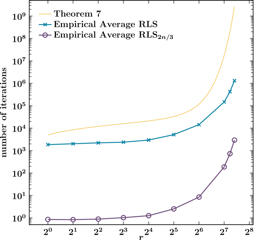
Figure 3: The theoretical (top, orange curve) and empirical expected run time of RLS (center, blue curve with $\times$) and RLS_2n/3 (bottom, purple curve with $\circ$) on $\textsc{Majority}_{r}$ for $n=10\,000$ and $r\in\{2^{i}\mid i\in\{0\}\cup[7]\}\cup\{150,170\}$. The theoretical run time is the upper bound from Theorem 7. For the empirical run times, for each value of $r$ stated above, the average of $1000$ independent runs of RLS and of RLS_2n/3 with uniform initialization is depicted. For more information regarding RLS_2n/3, please see Section IV-A; the value $2n/3$ is near-optimal, as shown in Figure 5, resulting in a drastically improved run time.

III-A Run Time Results on HasMajority

In our proof of Theorem 6, we aim to apply the additive-drift theorem (Theorem 1). To this end, letting $\bm{x}$ denote the currently best individual of RLS in each iteration, we consider the distance $n/2+r-\max\{|\bm{x}|_{0},|\bm{x}|_{1}\}$ of the majority of bits of $\bm{x}$ to the optimum value $n/2+r$ of $\textsc{HasMajority}_{r}$. Since it becomes less likely to decrease this distance the smaller it is, we choose a potential function that scales the space exponentially, counteracting this decline in probability.

Proof of Theorem 6.

For all $t\in\mathds{N}$, let $X_{t}=\max\{|\bm{x}^{(t)}|_{0},|\bm{x}^{(t)}|_{1}\}$, and let $(\mathcal{F}_{t})_{t\in\mathds{N}}$ denote the natural filtration of $X$. In addition, let $g\colon[n/2..n]\to\mathds{R}_{\geq 0}$ with

$$m\mapsto\begin{cases}\lambda^{r}-\lambda^{m-n/2}&:m<n/2+r\,,\\ 0&:\textrm{otherwise.}\end{cases}$$

Last, let $T=\inf\{t\in\mathds{N}\mid g(X_{t})=0\}$, and note that $T$ is a stopping time with respect to $\mathcal{F}$ and that it denotes the first point in time such that RLS found an optimum of $\textsc{HasMajority}_{r}$, as $X_{T}\geq n/2+r$. We show that $g(X)$ satisfies eq. 1 with $\mathcal{F}$ and $T$. Theorem 1 then yields the desired bound.

Let $t\in\mathds{N}$, and assume that $t<T$, as eq. 1 is trivially satisfied otherwise. Note that $X_{t}$ increases by $1$ if a bit that is not the strict majority in $\bm{x}^{(t)}$ is chosen to be flipped, which happens with probability $(n-X_{t})/n$ if $X_{t}>n/2$, and with probability $1$ if $X_{t}=n/2$. With the remaining probability, $X_{t}$ decreases by $1$.

For $X_{t}=n/2$, we get

$$g(X_{t})-\mathrm{E}\mathopen{}\mathclose{{}\left[{g(X_{t+1})\ \mathopen{}\mathclose{{}\left|\ \vphantom{g(X_{t+1})}\mathcal{F}_{t}}\right.}}\right] =\lambda^{r}-1-\mathopen{}\mathclose{{}\left(\lambda^{r}-\lambda}\right)=\lambda-1.$$ (7)

For the remaining case $X_{t}\in[n/2+1..n/2+r-1]$, we get

$$g(X_{t})-\mathrm{E}\mathopen{}\mathclose{{}\left[{g(X_{t+1})\ \mathopen{}\mathclose{{}\left|\ \vphantom{g(X_{t+1})}\mathcal{F}_{t}}\right.}}\right]$$

$$\quad=\lambda^{r}-\lambda^{X_{t}-n/2}-\mathopen{}\mathclose{{}\left(\lambda^{r}-\lambda^{X_{t}-1-n/2}}\right)\frac{X_{t}}{n}$$

$$\qquad-\mathopen{}\mathclose{{}\left(\lambda^{r}-\lambda^{X_{t}+1-n/2}}\right)\frac{n-X_{t}}{n}$$

$$\quad=\lambda^{X_{t}-n/2}\Big{(}\underbrace{\frac{1}{\lambda}\cdot\frac{X_{t}}{n}+\lambda\cdot\frac{n-X_{t}}{n}}_{\eqqcolon A}-1\Big{)}.$$ (8)

Let $b=2(r-1)$, $a=3r(n-b)(n+b)/\big{(}3r(n-b)-2n\big{)}$, and note that $\lambda=a/(n-b)$. Since $\lambda$ is greater than $1$, it follows that $A$ is decreasing in $X_{t}$ and thus minimal for $X_{t}=n/2+r-1=(n+b)/2$. Substituting $\lambda=a/(n-b)$, this yields

$$A \geq\frac{n-b}{a}\cdot\frac{n+b}{2n}+\frac{a}{n-b}\cdot\frac{n-b}{2n}$$ (9)

$$=\frac{(n-b)(n+b)+a^{2}}{2an}=\underbrace{\frac{n^{2}-b^{2}}{2an}}_{\eqqcolon B}+\frac{a}{2n}.$$

Noting that $a=3r(n^{2}-b^{2})/\big{(}3r(n-b)-2n\big{)}$, we get

$$B =\frac{3r(n-b)-2n}{2n\cdot 3r}=\frac{n-b}{2n}-\frac{1}{3r}.$$

Substituting this back into eq. 9 yields

$$A\geq\underbrace{\frac{a+n-b}{2n}}_{\eqqcolon C}-\frac{1}{3r}.$$ (10)

Again, by substituting $a=3r(n-b)(n+b)/(3r(n-b)-2n)$, we get

$$C =\frac{1}{2n}\mathopen{}\mathclose{{}\left(\frac{3r(n-b)(n+b)}{3r(n-b)-2n}+\frac{(n-b)\big{(}3r(n-b)-2n\big{)}}{3r(n-b)-2n}}\right)$$

$$=\frac{n-b}{2n}\cdot\frac{3r(n+b+n-b)-2n}{3r(n-b)-2n}=\frac{3r(n-b)-(n-b)}{3r(n-b)-2n}$$

$$=1+\frac{n+b}{3r(n-b)-2n}=1+\frac{1}{3r}\cdot\frac{3r(n+b)}{3r(n-b)-2n}$$

$$=1+\frac{a}{n-b}\cdot\frac{1}{3r}.$$

Substituting this back into eq. 10 and recalling that $\lambda=a/(n-b)$ yields $A\geq 1+(\lambda-1)/(3r)$. Substituting this bound into eq. 8 ultimately yields

$$g(X_{t})-\mathrm{E}\mathopen{}\mathclose{{}\left[{g(X_{t+1})\ \mathopen{}\mathclose{{}\left|\ \vphantom{g(X_{t+1})}\mathcal{F}_{t}}\right.}}\right]\geq\lambda^{X_{t}-n/2}\cdot(\lambda-1)\cdot\frac{1}{3r}.$$ (11)

Applying Theorem 1 with $\delta=(\lambda-1)/(3r)$ being the minimum of eqs. 7 and 11 and noting that $\mathrm{E}\mathopen{}\mathclose{{}\left[{g(X_{T})\ \mathopen{}\mathclose{{}\left|\ \vphantom{g(X_{T})}\mathcal{F}_{0}}\right.}}\right]=0$ concludes the proof. ∎

III-B Run Time Results on Majority

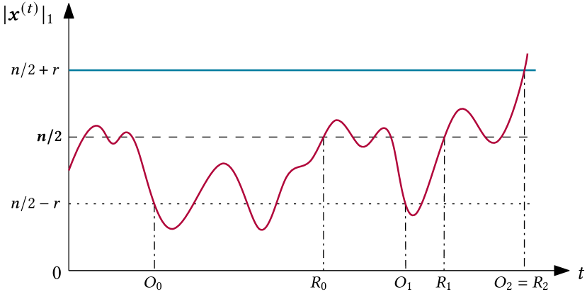
Figure 4: A visualization of the definitions of the random variables $(O_{i})_{i\in\mathds{N}}$ and $(R_{i})_{i\in\mathds{N}}$ as defined in eq. 12, needed for Corollary 9. The red wavy line depicts an example of how the number of $1$s in the best solution of an EA (given by the sequence $(\bm{x}^{(t)})_{t\in\mathds{N}}$) changes over time ($t$). For the sake of readability, we depict this line as continuous although it is discrete and can have jumps. The stopping times $(O_{i})_{i\in\mathds{N}}$ and $(R_{i})_{i\in\mathds{N}}$ always alternate, by definition.

We show how to derive a run time bound of an EA $A$ for Majority based on a run time bound for HasMajority (Corollary 9). The argument is based on the observation that whenever $A$ finds an optimum of HasMajority, this solution can also be an optimum of Majority. If this is not the case, that is, if the current solution has a majority of $0$s, we wait until $A$ gets back to a solution of at least $n/2$ $1$s. Then, we wait again until it finds an optimum of HasMajority, repeating this argument until $A$ finds an optimum of Majority.

More formally, we define the following two interleaving sequences of stopping times, which we also visualize in Figure 4:

$$O_{0} =\inf\{t\in\mathds{N}\mid\textsc{HasMajority}_{r}(\bm{x}^{(t)})=1\}\ ,$$ (12)

as well as, for all $$i\in\mathds{N}$$,

$$R_{i} =\inf\{t\in\mathds{N}\mid t\geq O_{i}\land|\bm{x}^{(t)}|_{1}\geq n/2\}\ \textrm{, and}$$

$$O_{i+1} =\inf\{t\in\mathds{N}\mid t>R_{i}\land\textsc{HasMajority}_{r}(\bm{x}^{(t)})=1\}.$$

The sequence $O$ denotes the points in time (interleaved by $R$) where $A$ can have found an optimum of Majority, as it found an optimum of HasMajority. In the context of proving a run time bound for Majority, $O$ denotes the points in time from where we wait until $A$ returns to an individual with at least as many $1$s as $0$s in order to repeat our argument. The sequence $R$ denotes those points in time where we repeat our argument. Theorem 5 formalizes this argument and yields a bound on the overall expected run time on Majority.

Since the idea of this argument holds for any interleaved assortment of stopping times, we first prove a more general theorem (Theorem 8) before we state the result specific to our setting (Corollary 9). This theorem generalizes the idea of the stopping times from eq. 12, but it does not specify their interpretation.

Theorem 8 (Decomposition argument).

Let $\mathopen{}\mathclose{{}\left(\mathcal{F}_{i}}\right)_{i\in\mathds{N}}$ be a filtration, let $S$ be a stopping time with respect to $\mathcal{F}$, and let $(O_{i})_{i\in\mathds{N}}$ and $(R_{i})_{i\in\mathds{N}}$ be stopping times with respect to $\mathcal{F}$ such that for all $i\in\mathds{N}$, it holds that $O_{i}\leq R_{i}<O_{i+1}$. Moreover, let $U=\sup\{i\in\mathds{N}\mid O_{i}\leq S\}$, and assume that there is a $p_{0}\in(0,1]$ such that $\mathrm{Pr}\mathopen{}\mathclose{{}\left[{O_{0}=S}}\right]=p_{0}$.

Assume that $\sum_{i\in[U]}(O_{i}-O_{i-1})$ and $U$ are integrable as well as that there is a $c\in\mathds{R}$ such that for all $i\in\mathds{N}_{>0}$, it holds that $\mathrm{E}\mathopen{}\mathclose{{}\left[{|O_{i}-\mathrm{E}\mathopen{}\mathclose{{}\left[{O_{i}\ \mathopen{}\mathclose{{}\left|\ \vphantom{O_{i}}\mathcal{F}_{R_{i-1}}}\right.}}\right]|\ \mathopen{}\mathclose{{}\left|\ \vphantom{|O_{i}-\mathrm{E}\mathopen{}\mathclose{{}\left[{O_{i}\ \mathopen{}\mathclose{{}\left|\ \vphantom{O_{i}}\mathcal{F}_{R_{i-1}}}\right.}}\right]|}\mathcal{F}_{R_{i-1}}}\right.}}\right]\leq c$ and $\mathrm{E}\mathopen{}\mathclose{{}\left[{|R_{i-1}-\mathrm{E}\mathopen{}\mathclose{{}\left[{R_{i-1}\ \mathopen{}\mathclose{{}\left|\ \vphantom{R_{i-1}}\mathcal{F}_{O_{i-1}}}\right.}}\right]|\ \mathopen{}\mathclose{{}\left|\ \vphantom{|R_{i-1}-\mathrm{E}\mathopen{}\mathclose{{}\left[{R_{i-1}\ \mathopen{}\mathclose{{}\left|\ \vphantom{R_{i-1}}\mathcal{F}_{O_{i-1}}}\right.}}\right]|}\mathcal{F}_{O_{i-1}}}\right.}}\right]\leq c$.

Last, let $L$ denote the event that $U\geq 1$. Then

$$\mathrm{E}\mathopen{}\mathclose{{}\left[{S}}\right] =\mathrm{E}\mathopen{}\mathclose{{}\left[{O_{0}}}\right]+(1-p_{0})\mathrm{E}\Big{[}\sum\nolimits_{i\in[U]}\big{(}\mathrm{E}\mathopen{}\mathclose{{}\left[{O_{i}-R_{i-1}\ \mathopen{}\mathclose{{}\left|\ \vphantom{O_{i}-R_{i-1}}\mathcal{F}_{R_{i-1}}}\right.}}\right]$$

$$\hskip 88.2037pt+\mathrm{E}\mathopen{}\mathclose{{}\left[{R_{i-1}-O_{i-1}\ \mathopen{}\mathclose{{}\left|\ \vphantom{R_{i-1}-O_{i-1}}\mathcal{F}_{O_{i-1}}}\right.}}\right]\big{)}\,\Big{|}\,L\Big{]}\,,$$

where we interpret the second summand to be $0$ if $1-p_{0}=0$.

Proof.

We aim to express $S$ as a sum of time intervals that reflect the repeats as outlined at the beginning of Section III-B. To this end, for all $i\in\mathds{N}_{>0}$, let $\Delta_{i}=O_{i}-O_{i-1}$. Note that this implies that $S=T+\sum_{i\in[U]}\Delta_{i}$, since $T=O_{0}$, $S=O_{U}$, and the sum is telescoping.

By the linearity of expectation, it follows that $\mathrm{E}\mathopen{}\mathclose{{}\left[{S}}\right]=\mathrm{E}\mathopen{}\mathclose{{}\left[{T}}\right]+\mathrm{E}\mathopen{}\mathclose{{}\left[{\sum_{i\in[U]}\Delta_{i}}}\right]$. Note that $\mathrm{E}\big{[}{\sum_{i\in[U]}\Delta_{i}\ \big{|}\ \vphantom{\sum_{i\in[U]}\Delta_{i}}\overline{L}}\big{]}=0$ as well as $\mathrm{Pr}\mathopen{}\mathclose{{}\left[{L}}\right]=1-p_{0}$. Thus, $\mathrm{E}\mathopen{}\mathclose{{}\left[{\sum_{i\in[U]}\Delta_{i}}}\right]=(1-p_{0})\mathrm{E}\mathopen{}\mathclose{{}\left[{\sum_{i\in[U]}\Delta_{i}\ \mathopen{}\mathclose{{}\left|\ \vphantom{\sum_{i\in[U]}\Delta_{i}}L}\right.}}\right]$, which is $0$ if $\mathrm{Pr}\mathopen{}\mathclose{{}\left[{L}}\right]=0$.

Let $i\in\mathds{N}_{>0}$, and note that, $\Delta_{i}=O_{i}-O_{i-1}=(O_{i}-R_{i-1})+(R_{i-1}-O_{i-1})$. Thus, by the linearity of expectation,

$$\mathrm{E}\mathopen{}\mathclose{{}\left[{\sum\nolimits_{i\in[U]}\Delta_{i}\ \mathopen{}\mathclose{{}\left|\ \vphantom{\sum\nolimits_{i\in[U]}\Delta_{i}}L}\right.}}\right] =\mathrm{E}\mathopen{}\mathclose{{}\left[{\sum\nolimits_{i\in[U]}(O_{i}-R_{i-1})\ \mathopen{}\mathclose{{}\left|\ \vphantom{\sum\nolimits_{i\in[U]}(O_{i}-R_{i-1})}L}\right.}}\right]$$

$$\quad+\mathrm{E}\mathopen{}\mathclose{{}\left[{\sum\nolimits_{i\in[U]}(R_{i-1}-O_{i-1})\ \mathopen{}\mathclose{{}\left|\ \vphantom{\sum\nolimits_{i\in[U]}(R_{i-1}-O_{i-1})}L}\right.}}\right].$$

We aim to apply Theorem 5 to both expected values on the right-hand side with $U$ and a suitable filtration. To this end, let

$$(M_{\textrm{$i$}})_{i\in\mathds{N}_{>0}}=(O_{i+1}-R_{i})_{i\in\mathds{N}}\textrm{\,and\,}(N_{\textrm{$i$}})_{i\in\mathds{N}_{>0}}=(R_{i}-O_{i})_{i\in\mathds{N}},$$

and note that the indices of the new sequences start at $1$ whereas they start at $0$ for the old ones. Note that $U$ is integrable by assumption.

Considering $M_{\textrm{}}$: Let $(\mathcal{G}_{i})_{i\in\mathds{N}}=(\mathcal{F}_{\inf\{R_{i},S\}})_{i\in\mathds{N}}$. Note that $(M_{\textrm{$i$}}\cdot\mathds{1}{(i\leq U)})_{i\in\mathds{N}_{>0}}$ is adapted to $\mathcal{G}$, as for all $i\in\mathds{N}_{>0}$, it holds that $R_{i-1}\cdot\mathds{1}{(i\leq U)}<O_{i}\cdot\mathds{1}{(i\leq U)}\leq\inf\{R_{i},S\}$ and thus that $M_{\textrm{$i$}}\cdot\mathds{1}{(i\leq U)}$ is $\mathcal{G}_{i}$-measurable.

Since $\sum_{i\in[U]}(O_{i}-O_{i-1})=\sum_{i\in[U]}M_{\textrm{$i$}}+\sum_{i\in[U]}N_{\textrm{$i$}}$ is integrable by assumption, and since $M_{\textrm{}}$ and $N_{\textrm{}}$ are non-negative by the definition of $O$ and $R$, it follows that $\sum_{i\in[U]}M_{\textrm{$i$}}$ is integrable. Further, since $(1)$ $R_{i-1}$ is $\mathcal{F}_{R_{i-1}}$-measurable, and $(2)$ by the assumption that there is a $c\in\mathds{R}$ such that for all $i\in\mathds{N}_{>0}$, we have $\mathrm{E}\mathopen{}\mathclose{{}\left[{|O_{i}-\mathrm{E}\mathopen{}\mathclose{{}\left[{O_{i}\ \mathopen{}\mathclose{{}\left|\ \vphantom{O_{i}}\mathcal{F}_{R_{i-1}}}\right.}}\right]|\ \mathopen{}\mathclose{{}\left|\ \vphantom{|O_{i}-\mathrm{E}\mathopen{}\mathclose{{}\left[{O_{i}\ \mathopen{}\mathclose{{}\left|\ \vphantom{O_{i}}\mathcal{F}_{R_{i-1}}}\right.}}\right]|}\mathcal{F}_{R_{i-1}}}\right.}}\right]\leq c$,

$$\mathrm{E}\mathopen{}\mathclose{{}\left[{|M_{\textrm{$i$}}-\mathrm{E}\mathopen{}\mathclose{{}\left[{M_{\textrm{$i$}}\ \mathopen{}\mathclose{{}\left|\ \vphantom{M_{\textrm{$i$}}}\mathcal{F}_{R_{i-1}}}\right.}}\right]|\ \mathopen{}\mathclose{{}\left|\ \vphantom{|M_{\textrm{$i$}}-\mathrm{E}\mathopen{}\mathclose{{}\left[{M_{\textrm{$i$}}\ \mathopen{}\mathclose{{}\left|\ \vphantom{M_{\textrm{$i$}}}\mathcal{F}_{R_{i-1}}}\right.}}\right]|}\mathcal{F}_{R_{i-1}}}\right.}}\right]$$

$$=\mathrm{E}\mathopen{}\mathclose{{}\left[{|O_{i}-R_{i-1}-\mathrm{E}\mathopen{}\mathclose{{}\left[{O_{i}-R_{i-1}\ \mathopen{}\mathclose{{}\left|\ \vphantom{O_{i}-R_{i-1}}\mathcal{F}_{R_{i-1}}}\right.}}\right]|\ \mathopen{}\mathclose{{}\left|\ \vphantom{|O_{i}-R_{i-1}-\mathrm{E}\mathopen{}\mathclose{{}\left[{O_{i}-R_{i-1}\ \mathopen{}\mathclose{{}\left|\ \vphantom{O_{i}-R_{i-1}}\mathcal{F}_{R_{i-1}}}\right.}}\right]|}\mathcal{F}_{R_{i-1}}}\right.}}\right]$$

$$\overset{(1)}{=}\mathrm{E}\mathopen{}\mathclose{{}\left[{|O_{i}-\mathrm{E}\mathopen{}\mathclose{{}\left[{O_{i}\ \mathopen{}\mathclose{{}\left|\ \vphantom{O_{i}}\mathcal{F}_{R_{i-1}}}\right.}}\right]|\ \mathopen{}\mathclose{{}\left|\ \vphantom{|O_{i}-\mathrm{E}\mathopen{}\mathclose{{}\left[{O_{i}\ \mathopen{}\mathclose{{}\left|\ \vphantom{O_{i}}\mathcal{F}_{R_{i-1}}}\right.}}\right]|}\mathcal{F}_{R_{i-1}}}\right.}}\right]\overset{(2)}{\leq}c.$$

Since, for all $i\in\mathds{N}_{>0}$ such that $i\leq U$, it holds that $R_{i-1}<S$, it follows for all $i\in\mathds{N}_{>0}$ that

$$\mathrm{E}\mathopen{}\mathclose{{}\left[{|M_{\textrm{$i$}}-\mathrm{E}\mathopen{}\mathclose{{}\left[{M_{\textrm{$i$}}\ \mathopen{}\mathclose{{}\left|\ \vphantom{M_{\textrm{$i$}}}\mathcal{G}_{i-1}}\right.}}\right]|\ \mathopen{}\mathclose{{}\left|\ \vphantom{|M_{\textrm{$i$}}-\mathrm{E}\mathopen{}\mathclose{{}\left[{M_{\textrm{$i$}}\ \mathopen{}\mathclose{{}\left|\ \vphantom{M_{\textrm{$i$}}}\mathcal{G}_{i-1}}\right.}}\right]|}\mathcal{G}_{i-1}}\right.}}\right]\cdot\mathds{1}{(i-1<U)}\leq c.$$

Applying Theorem 5 and taking the expectations on both sides yields $\mathrm{E}\Big{[}{\sum\nolimits_{i\in[U]}M_{\textrm{$i$}}\ \Big{|}\ \vphantom{\sum\nolimits_{i\in[U]}M_{\textrm{$i$}}}L}\Big{]}=\mathrm{E}\Big{[}{\sum\nolimits_{i\in[U]}\mathrm{E}\mathopen{}\mathclose{{}\left[{M_{\textrm{$i$}}\ \mathopen{}\mathclose{{}\left|\ \vphantom{M_{\textrm{$i$}}}\mathcal{G}_{i-1}}\right.}}\right]\ \Big{|}\ \vphantom{\sum\nolimits_{i\in[U]}\mathrm{E}\mathopen{}\mathclose{{}\left[{M_{\textrm{$i$}}\ \mathopen{}\mathclose{{}\left|\ \vphantom{M_{\textrm{$i$}}}\mathcal{G}_{i-1}}\right.}}\right]missing}L}\Big{]}$.

Considering $N_{\textrm{}}$: This case is very similar to the previous one. Let $(\mathcal{G}_{i})_{i\in\mathds{N}}=(\mathcal{F}_{\inf\{O_{i},S\}})_{i\in\mathds{N}}$. Note that $(N_{\textrm{$i$}}\cdot\mathds{1}{(i\leq U)})_{i\in\mathds{N}_{>0}}$ is adapted to $\mathcal{G}$, as for all $i\in\mathds{N}_{>0}$, it holds that $O_{i-1}\cdot\mathds{1}{(i\leq U)}\leq R_{i-1}\cdot\mathds{1}{(i\leq U)}<\inf\{O_{i},S\}$. Further, as in the previous case, since $\sum_{i\in[U]}(O_{i}-O_{i-1})$ is integrable by assumption, so is $\sum_{i\in[U]}N_{\textrm{$i$}}$. Last, by the assumption that there is a $c\in\mathds{R}$ such that for all $i\in\mathds{N}_{>0}$, it holds that $\mathrm{E}\mathopen{}\mathclose{{}\left[{|R_{i-1}-\mathrm{E}\mathopen{}\mathclose{{}\left[{R_{i-1}\ \mathopen{}\mathclose{{}\left|\ \vphantom{R_{i-1}}\mathcal{F}_{O_{i-1}}}\right.}}\right]|\ \mathopen{}\mathclose{{}\left|\ \vphantom{|R_{i-1}-\mathrm{E}\mathopen{}\mathclose{{}\left[{R_{i-1}\ \mathopen{}\mathclose{{}\left|\ \vphantom{R_{i-1}}\mathcal{F}_{O_{i-1}}}\right.}}\right]|}\mathcal{F}_{O_{i-1}}}\right.}}\right]\leq c$, and since for all $i\in\mathds{N}_{>0}$ such that $i\leq U$ it holds that $O_{i-1}<S$, it follows for all $i\in\mathds{N}_{>0}$, by adding $O_{i-1}-O_{i-1}$ inside the expectation, that $\mathrm{E}\mathopen{}\mathclose{{}\left[{|N_{\textrm{$i$}}-\mathrm{E}\mathopen{}\mathclose{{}\left[{N_{\textrm{$i$}}\ \mathopen{}\mathclose{{}\left|\ \vphantom{N_{\textrm{$i$}}}\mathcal{G}_{i-1}}\right.}}\right]|\ \mathopen{}\mathclose{{}\left|\ \vphantom{|N_{\textrm{$i$}}-\mathrm{E}\mathopen{}\mathclose{{}\left[{N_{\textrm{$i$}}\ \mathopen{}\mathclose{{}\left|\ \vphantom{N_{\textrm{$i$}}}\mathcal{G}_{i-1}}\right.}}\right]|}\mathcal{G}_{i-1}}\right.}}\right]\cdot\mathds{1}{(i-1<U)}\leq c$. Applying Theorem 5 and taking the expectations on both sides yields $\mathrm{E}\mathopen{}\mathclose{{}\left[{\sum_{i\in[U]}N_{\textrm{$i$}}\ \mathopen{}\mathclose{{}\left|\ \vphantom{\sum_{i\in[U]}N_{\textrm{$i$}}}L}\right.}}\right]=\mathrm{E}\mathopen{}\mathclose{{}\left[{\sum\nolimits_{i\in[U]}\mathrm{E}\mathopen{}\mathclose{{}\left[{N_{\textrm{$i$}}\ \mathopen{}\mathclose{{}\left|\ \vphantom{N_{\textrm{$i$}}}\mathcal{G}_{i-1}}\right.}}\right]\ \mathopen{}\mathclose{{}\left|\ \vphantom{\sum\nolimits_{i\in[U]}\mathrm{E}\mathopen{}\mathclose{{}\left[{N_{\textrm{$i$}}\ \mathopen{}\mathclose{{}\left|\ \vphantom{N_{\textrm{$i$}}}\mathcal{G}_{i-1}}\right.}}\right]missing}L}\right.}}\right]$.

Concluding: Taking everything together and noting that for all $i\in\mathds{N}_{>0}$ such that $i\leq U$ it holds that $R_{i-1}<S$ and that $O_{i-1}<S$ concludes the proof. ∎

With respect to our setting, utilizing the definitions from eq. 12, we get the following result.

Corollary 9 (Translating results from HasMajority to Majority).

Let $n\in\mathds{N}_{>0}$ be even, let $r\in[n/2]$, and let $D$ be a distribution over $\{0,1\}^{n}$. Consider an EA $A$, respresented by the sequence $(\bm{x}^{(t)})_{t\in\mathds{N}}$ with initialization distribution $D$, adapted to a filtration $\mathopen{}\mathclose{{}\left(\mathcal{F}_{i}}\right)_{i\in\mathds{N}}$.

Assume that when $A$ optimizes $\textsc{HasMajority}_{r}$, there is a probability $p_{0}\in(0,1]$ that this solution is also an optimum of Majority. Furthermore, assume the definitions of eq. 12.

Let $S$ denote the run time of $A$ on $\textsc{Majority}_{r}$, and let $U=\sup\{i\in\mathds{N}\mid O_{i}\leq S\}$. Assume that $\sum_{i\in[U]}(O_{i}-O_{i-1})$ and $U$ are integrable as well as that there is a $c\in\mathds{R}$ such that for all $i\in\mathds{N}_{>0}$, it holds that $\mathrm{E}\mathopen{}\mathclose{{}\left[{|O_{i}-\mathrm{E}\mathopen{}\mathclose{{}\left[{O_{i}\ \mathopen{}\mathclose{{}\left|\ \vphantom{O_{i}}\mathcal{F}_{R_{i-1}}}\right.}}\right]|\ \mathopen{}\mathclose{{}\left|\ \vphantom{|O_{i}-\mathrm{E}\mathopen{}\mathclose{{}\left[{O_{i}\ \mathopen{}\mathclose{{}\left|\ \vphantom{O_{i}}\mathcal{F}_{R_{i-1}}}\right.}}\right]|}\mathcal{F}_{R_{i-1}}}\right.}}\right]\leq c$ and $\mathrm{E}\mathopen{}\mathclose{{}\left[{|R_{i-1}-\mathrm{E}\mathopen{}\mathclose{{}\left[{R_{i-1}\ \mathopen{}\mathclose{{}\left|\ \vphantom{R_{i-1}}\mathcal{F}_{O_{i-1}}}\right.}}\right]|\ \mathopen{}\mathclose{{}\left|\ \vphantom{|R_{i-1}-\mathrm{E}\mathopen{}\mathclose{{}\left[{R_{i-1}\ \mathopen{}\mathclose{{}\left|\ \vphantom{R_{i-1}}\mathcal{F}_{O_{i-1}}}\right.}}\right]|}\mathcal{F}_{O_{i-1}}}\right.}}\right]\leq c$.

Last, let $L$ denote the event that $U\geq 1$, and let $T$ denote the run time of $A$ on $\textsc{HasMajority}_{r}$. Then

$$\mathrm{E}\mathopen{}\mathclose{{}\left[{S}}\right] =\mathrm{E}\mathopen{}\mathclose{{}\left[{T}}\right]+(1-p_{0})\mathrm{E}\Big{[}\sum\nolimits_{i\in[U]}\big{(}\mathrm{E}\mathopen{}\mathclose{{}\left[{O_{i}-R_{i-1}\ \mathopen{}\mathclose{{}\left|\ \vphantom{O_{i}-R_{i-1}}\mathcal{F}_{R_{i-1}}}\right.}}\right]$$

$$\hskip 88.2037pt+\mathrm{E}\mathopen{}\mathclose{{}\left[{R_{i-1}-O_{i-1}\ \mathopen{}\mathclose{{}\left|\ \vphantom{R_{i-1}-O_{i-1}}\mathcal{F}_{O_{i-1}}}\right.}}\right]\big{)}\,\Big{|}\,L\Big{]}\,,$$

where we interpret the second summand to be $0$ if $1-p_{0}=0$.

Corollary 9 states an equality for the expected run time of an EA on Majority. Although calculating the exact expectations of the right-hand side generally seems implausible, the theorem can still be used in order to derive upper and lower bounds for expected run times on Majority by deriving corresponding bounds for all of the expected values in question. Using the notation of the theorem, an easy way for getting a bound on the expectation conditional on $L$ is to derive worst-case bounds for both of the conditional expectations in the sum. If these worst-case bounds are constants, then they can be pulled out of the expectation, and it remains to bound $\mathrm{E}\mathopen{}\mathclose{{}\left[{U\ \mathopen{}\mathclose{{}\left|\ \vphantom{U}L}\right.}}\right]$, which requires to only reason about the number of times of attempting to find an optimum of Majority when optimizing HasMajority. It is worth noting that the second of the conditional expectations in the sum considers the run time of $A$ optimizing HasMajority when starting with a solution with a majority of $1$s. Since this is typically very similar to how $T$ is defined, as only the initialization (and the history of $A$) differs between both scenarios, this expectation may already follow from a bound on $\mathrm{E}\mathopen{}\mathclose{{}\left[{T}}\right]$. Overall, the complexity of the run time analysis for Majority is drastically reduced.

In the following, we apply the technique above in order to derive run time bounds for RLS on Majority. Note that we already have an upper bound on the expected run time on HasMajority for arbitrary initializations, due to Theorem 6. Thus, we are only concerned with how often the algorithms find an optimum $\bm{x}$ of HasMajority with a majority of $0$s before optimizing Majority, and with how long it takes to get from $\bm{x}$ to a solution with a majority of $1$s. While the latter question is specific to each algorithm, we answer the former for all unbiased algorithms.

III-B1 Number of Retries

Using the notation of Corollary 9, we bound $\mathrm{E}\mathopen{}\mathclose{{}\left[{U\ \mathopen{}\mathclose{{}\left|\ \vphantom{U}D}\right.}}\right]$ from above for $(1+1)$-unary unbiased elitist algorithms with memory-restriction, as detailed in Algorithm 2. Further, we require the sequence of mutation operator $(\phi_{t})_{t\in\mathds{N}}$ of such an algorithm to be OneMax-compliant, which means that each mutation operator satisfies that results of individuals with many $1$s are at least as likely to have as many $1$s as results of individuals with fewer $1$s. Formally, we say that $\phi$ is OneMax-compliant if and only if, for all $t_{1},t_{2}\in\mathds{N}$, all $\bm{y},\bm{z}\in\{0,1\}^{n}$ with $\bm{y}=\bm{x}^{(t_{1})}$, $\bm{z}=\bm{x}^{(t_{2})}$, and $|\bm{y}|_{1}\leq|\bm{z}|_{1}$, and all $i\in[0..n]$, it holds that $\mathrm{Pr}\mathopen{}\mathclose{{}\left[{|\phi_{t_{1}}(\bm{y})|_{1}\geq i\ \mathopen{}\mathclose{{}\left|\ \vphantom{|\phi_{t_{1}}(\bm{y})|_{1}\geq i}\bm{y}}\right.}}\right]\leq\mathrm{Pr}\mathopen{}\mathclose{{}\left[{|\phi_{t_{2}}(\bm{z})|_{1}\geq i\ \mathopen{}\mathclose{{}\left|\ \vphantom{|\phi_{t_{2}}(\bm{z})|_{1}\geq i}\bm{z}}\right.}}\right]$. Note that while typical mutation operators are OneMax-compliant, operations such as the inversion of a bit string are not. This definition leads to the following result.

1 $\bm{x}^{(0)}\sim D$;

2 for $t\in\mathds{N}$ do

3       $\bm{y}\leftarrow\phi_{t}(\bm{x}^{(t)})$;

4       if $f(\bm{y})\geq f(\bm{x}^{(t)})$ then  $\bm{x}^{(t+1)}\leftarrow\bm{y}$;

5       else  $\bm{x}^{(t+1)}\leftarrow\bm{x}^{(t)}$;

6      

Algorithm 2 The $(1+1)$-unary unbiased algorithm framework with unbiased and memory-restricted mutation operators $(\phi_{t})_{t\in\mathds{N}}$ over $\{0,1\}^{n}$ and initial distribution $D$, maximizing function $f\colon\{0,1\}^{n}\to\mathds{R}$. Note for all $t\in\mathds{N}$ that $\phi_{t}$ only has access to a single individual, resulting in a heavy memory restriction.

Lemma 10.

Assume the setting of Corollary 9 and that $\mathcal{R}\coloneqq\{O_{i+1}-R_{i}\mid i\in\mathds{N}\land O_{i+1}\leq S\}$ is independent. If $A$ is an instance of Algorithm 2 with OneMax-compliant mutation $\phi$, then, conditional on $L$, it holds that $U$ is stochastically dominated by a geometrically distributed random variable with expectation $2$.

Proof.

Note that $|\mathcal{R}|=U$, and recall that $U\geq 1$, as we condition on $L$.

Let $i\in\mathds{N}$ such that $M_{i}\coloneqq O_{i+1}-R_{i}$ and $O_{i+1}\leq S$, that is, $M_{i}\in\mathcal{R}$. We call such an element a retry. We say that $M_{i}$ is a success if $O_{i+1}=S$, and a failure otherwise. Note that $U$ is the number of retries until the first success and that, by assumption, the retries are mutually independent.

It remains to show that each retry has a probability of at least $1/2$ of being a success. To this end, let $i\in\mathds{N}$ such that $M_{i}$ is a retry. First, assume that $|\bm{x}^{(R_{i})}|_{1}=n/2$. Recall that the retry ends once $A$ finds an optimum of $\textsc{HasMajority}_{r}$. Since $A$ is unbiased, each trajectory of $\bm{x}$ that ends with a solution with a majority of $0$s has a symmetric trajectory (in the sense of swapping $0$s and $1$s) with equal probability that ends with a solution with a majority of $1$s. Thus, the probability of $M_{i}$ being a success is $1/2$.

Now, assume that $|\bm{x}^{(R_{i})}|_{1}>n/2$. Let $\bm{y}^{(0)}\in\{0,1\}^{n}$ such that $|\bm{y}^{(0)}|_{1}=n/2$, and, for all $t\in\mathds{N}$, let $\bm{y}^{(t+1)}=\phi_{t}(\bm{y}^{(t)})$. Since $\phi$ is OneMax-compliant, it holds for all $t\in\mathds{N}$ that $|\bm{x}^{(R_{i}+t)}|_{1}$ stochastically dominates $|\bm{y}^{(t)}|_{1}$. Thus, there exists a coupling such that for all $t\in\mathds{N}$, it holds that $|\bm{x}^{(R_{i}+t)}|_{1}\geq|\bm{y}^{(t)}|_{1}$ [20, Theorem $1.8.10$]. Thus, the probability of $M_{i}$ being a success is at least as large as the probability of the process $\bm{y}$ finding a solution with at least $n/2+r$ $1$s before finding a solution with at least that many $0$s. By the first case above, the probability of this event is $1/2$. This concludes the proof. ∎

We note that RLS uses OneMax-compliant mutation.

III-B2 Integrability of the Stopping Time

An important property to check in Corollary 9 is that $\sum_{i\in[U]}(O_{i}-O_{i-1})$ is integrable. To this end, it suffices to show that this random variable has some finite expectation, as the sum is non-negative. We do so by applying Theorem 1.

Lemma 11.

Assume the setting of Corollary 9. Let $(\mathcal{F}_{t})_{t\in\mathds{N}}$ denote the natural filtration of $\bm{x}$, and assume that there is a $p\in(0,1]$ such that, for all $t\in\mathds{N}$, it holds that

$$\mathrm{Pr}\big{[}{|\bm{x}^{(t+1)}|_{1}>|\bm{x}^{(t)}|_{1}\ \big{|}\ \vphantom{|\bm{x}^{(t+1)}|_{1}>|\bm{x}^{(t)}|_{1}}\mathcal{F}_{t}}\big{]}\cdot\mathds{1}{(t<S)}\geq p\!\cdot\!\mathds{1}{(t<S)}.$$ (13)

Then $\sum_{i\in[U]}(O_{i}-O_{i-1})$ is integrable.

Proof.

We aim to prove that $\mathrm{E}\mathopen{}\mathclose{{}\left[{S}}\right]$ is integrable via Theorem 1. Since $\sum_{i\in[U]}(O_{i}-O_{i-1})\leq S$ and the terms of the sum are non-negative, the claim then follows. Recall that we assume that $n\geq 2$.

Let $(X_{t})_{t\in\mathds{N}}=\big{(}(n/p)^{n}-(n/p)^{|\bm{x}^{(t)}|_{1}}\big{)}$, and note that $X$ is non-negative and adapted to $\mathcal{F}$. Further note that eq. 1 is satisfied for all $t\in\mathds{N}$, since, using eq. 13, $n\geq 2$, and $p\leq 1$, it follows that

$$\big{(}X_{t}-\mathrm{E}\mathopen{}\mathclose{{}\left[{X_{t+1}\ \mathopen{}\mathclose{{}\left|\ \vphantom{X_{t+1}}\mathcal{F}_{t}}\right.}}\right]\big{)}\cdot\mathds{1}{(t<T)}$$

$$\quad=\Bigg{(}\mathopen{}\mathclose{{}\left(\frac{n}{p}}\right)^{|\bm{x}^{(t+1)}|_{1}}-\mathopen{}\mathclose{{}\left(\frac{n}{p}}\right)^{|\bm{x}^{(t)}|_{1}}\Bigg{)}$$

$$\qquad\cdot\mathrm{Pr}\big{[}{|\bm{x}^{(t+1)}|_{1}<|\bm{x}^{(t)}|_{1}\ \big{|}\ \vphantom{|\bm{x}^{(t+1)}|_{1}<|\bm{x}^{(t)}|_{1}}\mathcal{F}_{t}}\big{]}\cdot\mathds{1}{(t<S)}$$

$$\qquad+\Bigg{(}\mathopen{}\mathclose{{}\left(\frac{n}{p}}\right)^{|\bm{x}^{(t+1)}|_{1}}-\mathopen{}\mathclose{{}\left(\frac{n}{p}}\right)^{|\bm{x}^{(t)}|_{1}}\Bigg{)}$$

$$\qquad\quad\cdot\mathrm{Pr}\big{[}{|\bm{x}^{(t+1)}|_{1}>|\bm{x}^{(t)}|_{1}\ \big{|}\ \vphantom{|\bm{x}^{(t+1)}|_{1}>|\bm{x}^{(t)}|_{1}}\mathcal{F}_{t}}\big{]}\cdot\mathds{1}{(t<S)}$$

$$\quad\geq\Bigg{(}1-\mathopen{}\mathclose{{}\left(\frac{n}{p}}\right)^{|\bm{x}^{(t)}|_{1}}\Bigg{)}\cdot\mathds{1}{(t<S)}$$

$$\qquad+\mathopen{}\mathclose{{}\left(\frac{n}{p}}\right)^{|\bm{x}^{(t)}|_{1}}\cdot\mathopen{}\mathclose{{}\left(\frac{n}{p}-1}\right)\cdot p\cdot\mathds{1}{(t<S)}$$

$$\quad=\Bigg{(}1+\mathopen{}\mathclose{{}\left(\frac{n}{p}}\right)^{|\bm{x}^{(t)}|_{1}}\cdot\mathopen{}\mathclose{{}\left(\frac{n}{p}-2}\right)\Bigg{)}\cdot\mathds{1}{(t<S)}$$

$$\quad\geq\mathds{1}{(t<S)}.$$

Applying Theorem 1 with $\delta=1$, noting that $\mathrm{E}\mathopen{}\mathclose{{}\left[{X_{S}}}\right]\geq 0$, and then taking the expectation yields a finite bound for $\mathrm{E}\mathopen{}\mathclose{{}\left[{S}}\right]$, concluding the proof. ∎

III-B3 Reaching a Majority of Ones

The only thing left in order to apply Corollary 9 is to bound the expected time it takes an algorithm to get from a solution with a majority of $0$s to one with a majority of $1$s.

Theorem 12.

Consider RLS optimizing $\textsc{Majority}_{0}$, and assume that the initial individual $\bm{x}^{(0)}$ has at least $n/2+1$ $0$s. Then the expected run time of RLS is at most $n\big{(}1+\ln(|\bm{x}^{(0)}|_{0}-n/2)\big{)}/2$.

Proof.

We aim to apply Theorem 2. To this end, let $(\bm{x}^{(t)})_{t\in\mathds{N}}$ denote the best individual of RLS after each iteration, and let $(X_{t})_{t\in\mathds{N}}$ be such that for all $t\in\mathds{N}$, it holds that $X_{t}=|\bm{x}^{(t)}|_{0}-n/2$. Further, let $\mathcal{F}$ be the natural filtration of $\bm{x}$, and let $T=\inf\{t\mid X_{t}<1\}$. Note that $T$ denotes the run time of RLS on $\textsc{Majority}^{(1)}_{0}$.

Since $X_{0}\geq 1$ by assumption, we are left to check eq. 2. Let $t\in\mathds{N}$, and assume that $t<T$. Note that then

$$X_{t}-\mathrm{E}\mathopen{}\mathclose{{}\left[{X_{t+1}\ \mathopen{}\mathclose{{}\left|\ \vphantom{X_{t+1}}\mathcal{F}_{t}}\right.}}\right] =-1\cdot\frac{n-|\bm{x}^{(t)}|_{0}}{n}+1\cdot\frac{|\bm{x}^{(t)}|_{0}}{n}$$

$$=\frac{2|\bm{x}^{(t)}|_{0}-n}{n}=\frac{2}{n}X_{t}.$$

Applying Theorem 2 with $\delta=2/n$ concludes the proof. ∎

III-B4 Deriving the Run Time Result

By combining the results from the previous sections, the run time bound on Majority follows straightforwardly.

Proof of Theorem 7.

We aim to apply Corollary 9. To this end, we check the assumptions of the theorem and use its notation.

Due to the uniform initialization and the symmetry of the mutation of RLS (with respect to the number of $0$s and $1$s), it holds that $p_{0}=1/2$. By Lemma 11, $\sum_{i\in[U]}(O_{i}-O_{i-1})$ is integrable, and by Lemma 10, using that $\mathrm{E}\mathopen{}\mathclose{{}\left[{U}}\right]\leq\mathrm{E}\mathopen{}\mathclose{{}\left[{U\ \mathopen{}\mathclose{{}\left|\ \vphantom{U}L}\right.}}\right]+\mathrm{E}\big{[}{U\ \big{|}\ \vphantom{U}\overline{L}}\big{]}$ and, by definition of $L$, that $\mathrm{E}\big{[}{U\ \big{|}\ \vphantom{U}\overline{L}}\big{]}=0$, it follows that $U$ is integrable. The last condition to check is that there is a $c\in\mathds{R}$ such that for all $i\in\mathds{N}_{>0}$, it holds that $\mathrm{E}\mathopen{}\mathclose{{}\left[{|O_{i}-\mathrm{E}\mathopen{}\mathclose{{}\left[{O_{i}\ \mathopen{}\mathclose{{}\left|\ \vphantom{O_{i}}\mathcal{F}_{R_{i-1}}}\right.}}\right]|\ \mathopen{}\mathclose{{}\left|\ \vphantom{|O_{i}-\mathrm{E}\mathopen{}\mathclose{{}\left[{O_{i}\ \mathopen{}\mathclose{{}\left|\ \vphantom{O_{i}}\mathcal{F}_{R_{i-1}}}\right.}}\right]|}\mathcal{F}_{R_{i-1}}}\right.}}\right]\leq c$ and $\mathrm{E}\mathopen{}\mathclose{{}\left[{|R_{i-1}-\mathrm{E}\mathopen{}\mathclose{{}\left[{R_{i-1}\ \mathopen{}\mathclose{{}\left|\ \vphantom{R_{i-1}}\mathcal{F}_{O_{i-1}}}\right.}}\right]|\ \mathopen{}\mathclose{{}\left|\ \vphantom{|R_{i-1}-\mathrm{E}\mathopen{}\mathclose{{}\left[{R_{i-1}\ \mathopen{}\mathclose{{}\left|\ \vphantom{R_{i-1}}\mathcal{F}_{O_{i-1}}}\right.}}\right]|}\mathcal{F}_{O_{i-1}}}\right.}}\right]\leq c$. Let $i\in\mathds{N}_{>0}$. For the first inequality, we note that, by the triangle inequality and Jensen’s inequality,

$$\mathrm{E}\mathopen{}\mathclose{{}\left[{|O_{i}-\mathrm{E}\mathopen{}\mathclose{{}\left[{O_{i}\ \mathopen{}\mathclose{{}\left|\ \vphantom{O_{i}}\mathcal{F}_{R_{i-1}}}\right.}}\right]|\ \mathopen{}\mathclose{{}\left|\ \vphantom{|O_{i}-\mathrm{E}\mathopen{}\mathclose{{}\left[{O_{i}\ \mathopen{}\mathclose{{}\left|\ \vphantom{O_{i}}\mathcal{F}_{R_{i-1}}}\right.}}\right]|}\mathcal{F}_{R_{i-1}}}\right.}}\right]$$

$$=\mathrm{E}\mathopen{}\mathclose{{}\left[{|O_{i}-R_{i-1}-\mathrm{E}\mathopen{}\mathclose{{}\left[{O_{i}-R_{i-1}\ \mathopen{}\mathclose{{}\left|\ \vphantom{O_{i}-R_{i-1}}\mathcal{F}_{R_{i-1}}}\right.}}\right]|\ \mathopen{}\mathclose{{}\left|\ \vphantom{|O_{i}-R_{i-1}-\mathrm{E}\mathopen{}\mathclose{{}\left[{O_{i}-R_{i-1}\ \mathopen{}\mathclose{{}\left|\ \vphantom{O_{i}-R_{i-1}}\mathcal{F}_{R_{i-1}}}\right.}}\right]|}\mathcal{F}_{R_{i-1}}}\right.}}\right]$$

$$\leq 2\mathrm{E}\mathopen{}\mathclose{{}\left[{|O_{i}-R_{i-1}|\ \mathopen{}\mathclose{{}\left|\ \vphantom{|O_{i}-R_{i-1}|}\mathcal{F}_{R_{i-1}}}\right.}}\right].$$

By Theorem 6, using its notation, it holds that

$$\mathrm{E}\mathopen{}\mathclose{{}\left[{|O_{i}-R_{i-1}|\ \mathopen{}\mathclose{{}\left|\ \vphantom{|O_{i}-R_{i-1}|}\mathcal{F}_{R_{i-1}}}\right.}}\right]\leq 3r\cdot h\big{(}\bm{x}^{(R_{i-1})}\big{)}/(\lambda-1).$$

Since, for all $\bm{x}\in\{0,1\}^{n}$, it holds that $h(\bm{x})\leq\lambda^{r}-1$, it follows overall that $\mathrm{E}\mathopen{}\mathclose{{}\left[{|O_{i}-\mathrm{E}\mathopen{}\mathclose{{}\left[{O_{i}\ \mathopen{}\mathclose{{}\left|\ \vphantom{O_{i}}\mathcal{F}_{R_{i-1}}}\right.}}\right]|\ \mathopen{}\mathclose{{}\left|\ \vphantom{|O_{i}-\mathrm{E}\mathopen{}\mathclose{{}\left[{O_{i}\ \mathopen{}\mathclose{{}\left|\ \vphantom{O_{i}}\mathcal{F}_{R_{i-1}}}\right.}}\right]|}\mathcal{F}_{R_{i-1}}}\right.}}\right]\leq 6r\cdot(\lambda^{r}-1)/(\lambda-1)\eqqcolon c_{1}$. Similarly, we see that

$$\mathrm{E}\mathopen{}\mathclose{{}\left[{|R_{i-1}-\mathrm{E}\mathopen{}\mathclose{{}\left[{R_{i-1}\ \mathopen{}\mathclose{{}\left|\ \vphantom{R_{i-1}}\mathcal{F}_{O_{i-1}}}\right.}}\right]|\ \mathopen{}\mathclose{{}\left|\ \vphantom{|R_{i-1}-\mathrm{E}\mathopen{}\mathclose{{}\left[{R_{i-1}\ \mathopen{}\mathclose{{}\left|\ \vphantom{R_{i-1}}\mathcal{F}_{O_{i-1}}}\right.}}\right]|}\mathcal{F}_{O_{i-1}}}\right.}}\right]$$

$$=\mathrm{E}\mathopen{}\mathclose{{}\left[{|R_{i-1}-O_{i-1}-\mathrm{E}\mathopen{}\mathclose{{}\left[{R_{i-1}-O_{i-1}\ \mathopen{}\mathclose{{}\left|\ \vphantom{R_{i-1}-O_{i-1}}\mathcal{F}_{O_{i-1}}}\right.}}\right]|\ \mathopen{}\mathclose{{}\left|\ \vphantom{|R_{i-1}-O_{i-1}-\mathrm{E}\mathopen{}\mathclose{{}\left[{R_{i-1}-O_{i-1}\ \mathopen{}\mathclose{{}\left|\ \vphantom{R_{i-1}-O_{i-1}}\mathcal{F}_{O_{i-1}}}\right.}}\right]|}\mathcal{F}_{O_{i-1}}}\right.}}\right]$$

$$\leq 2\mathrm{E}\mathopen{}\mathclose{{}\left[{|R_{i-1}-O_{i-1}|\ \mathopen{}\mathclose{{}\left|\ \vphantom{|R_{i-1}-O_{i-1}|}\mathcal{F}_{O_{i-1}}}\right.}}\right].$$

By Theorem 12, it holds that

$$\mathrm{E}\mathopen{}\mathclose{{}\left[{|R_{i-1}-O_{i-1}|\ \mathopen{}\mathclose{{}\left|\ \vphantom{|R_{i-1}-O_{i-1}|}\mathcal{F}_{O_{i-1}}}\right.}}\right]\leq\tfrac{n}{2}\big{(}1+\ln(|\bm{x}^{(O_{i-1})}|_{0}-n/2)\big{)}.$$

Noting that $|\bm{x}^{(O_{i-1})}|_{0}=n/2+r$, since RLS cannot get to a solution with strictly more than $n/2+r$ $0$s before getting exactly $n/2+r$ $0$s, we get $\mathrm{E}\mathopen{}\mathclose{{}\left[{|R_{i-1}-\mathrm{E}\mathopen{}\mathclose{{}\left[{R_{i-1}\ \mathopen{}\mathclose{{}\left|\ \vphantom{R_{i-1}}\mathcal{F}_{O_{i-1}}}\right.}}\right]|\ \mathopen{}\mathclose{{}\left|\ \vphantom{|R_{i-1}-\mathrm{E}\mathopen{}\mathclose{{}\left[{R_{i-1}\ \mathopen{}\mathclose{{}\left|\ \vphantom{R_{i-1}}\mathcal{F}_{O_{i-1}}}\right.}}\right]|}\mathcal{F}_{O_{i-1}}}\right.}}\right]\leq n\big{(}1+\ln(r)\big{)}\eqqcolon c_{2}$. Thus, choosing $c=\max\{c_{1},c_{2}\}$ satisfies the remaining condition of Corollary 9.

We continue with bounding $\mathrm{E}\mathopen{}\mathclose{{}\left[{T}}\right]$, noting that for all $i\in\mathds{N}_{>0}$ such that $i\in[U]$, we bounded the expectations $\mathrm{E}\mathopen{}\mathclose{{}\left[{O_{i}-R_{i-1}\ \mathopen{}\mathclose{{}\left|\ \vphantom{O_{i}-R_{i-1}}\mathcal{F}_{R_{i-1}}}\right.}}\right]$ and $\mathrm{E}\mathopen{}\mathclose{{}\left[{R_{i-1}-O_{i-1}\ \mathopen{}\mathclose{{}\left|\ \vphantom{R_{i-1}-O_{i-1}}\mathcal{F}_{O_{i-1}}}\right.}}\right]$ already above, as the differences are non-negative and the absolute value thus does not change anything.

Let $i\in\mathds{N}_{>0}$ such that $i\in[U]$. Note that $O_{i}-R_{i-1}$ and $T$ have the same distribution conditional on the same initial individual for the respective time interval, since RLS is Markovian and since both stopping times stop once an optimum of $\textsc{HasMajority}_{r}$ is found. Thus, their conditional expectations (on the same initial individual) are the same, and Theorem 6 yields a bound for $\mathrm{E}\mathopen{}\mathclose{{}\left[{T}}\right]$, too.

Combining all bounds, by the tower rule for expectation, Corollary 9 yields

$$\mathrm{E}\mathopen{}\mathclose{{}\left[{S}}\right] \leq 3r\cdot\frac{\lambda^{r}-1}{\lambda-1}$$

$$\quad+\frac{1}{2}\mathrm{E}\mathopen{}\mathclose{{}\left[{\sum\nolimits_{i\in[U]}\mathopen{}\mathclose{{}\left(n\frac{1+\ln(r)}{2}+3r\cdot\frac{\lambda^{r}-1}{\lambda-1}}\right)\ \mathopen{}\mathclose{{}\left|\ \vphantom{\sum\nolimits_{i\in[U]}\mathopen{}\mathclose{{}\left(n\frac{1+\ln(r)}{2}+3r\cdot\frac{\lambda^{r}-1}{\lambda-1}}\right)}L}\right.}}\right]$$

$$=3r\cdot\frac{\lambda^{r}-1}{\lambda-1}+\frac{1}{2}\mathopen{}\mathclose{{}\left(n\frac{1+\ln(r)}{2}+3r\cdot\frac{\lambda^{r}-1}{\lambda-1}}\right)\mathrm{E}\mathopen{}\mathclose{{}\left[{U\ \mathopen{}\mathclose{{}\left|\ \vphantom{U}L}\right.}}\right].$$

Applying Lemma 10 yields $\mathrm{E}\mathopen{}\mathclose{{}\left[{U\ \mathopen{}\mathclose{{}\left|\ \vphantom{U}L}\right.}}\right]\leq 2$, thus concluding the proof. ∎

III-C Results for Neutrality in the W-Model

For all $n\in\mathds{N}_{>0}$, all $\bm{x}\in\{0,1\}^{n}$, and all $S\subseteq[n]$, let $\bm{x}_{S}$ denote the bit string of length $|S|$ that consists only of those entries in $\bm{x}$ with an index in $S$, that is, $\bm{x}_{S}=(\bm{x}_{i})_{i\in S}$.

Let $n\in\mathds{N}_{>0}$. Given a pseudo-Boolean function $f\colon\{0,1\}^{n}\to\mathds{R}$ as well as $k\in\mathds{N}_{>0}$, the property of neutrality in the W-model [1] constructs a new function $f^{\prime}\colon\{0,1\}^{nk}\to\mathds{R}$ with

$$\bm{x}\mapsto f\big{(}\textsc{Majority}_{1}(\bm{x}_{[(i-1)k+1..ik]})_{i\in[n]}\big{)}.$$

In other words, each bit of $f$ is exchanged for a block of $k$ bits. When evaluating $f^{\prime}$, for each block, the majority of bits is determined, and then $f$ is evaluated on the string of the $n$ majority bits. We refer to $f^{\prime}$ as $d$ with added neutrality of degree $k$.

Applying the results by Doerr et al. [2], we get the following bound for the expected run time of RLS on the pseudo-Boolean function $\textsc{OneMax}\colon\bm{x}\mapsto|\bm{x}|_{1}$ with added neutrality.

Corollary 13.

Let $n,k\in\mathds{N}_{>0}$ such that $n$ is even. For sufficiently large $n$, the expected run time of RLS on OneMax with added neutrality of degree $k$ is at most $\mathrm{O}\mathopen{}\mathclose{{}\left({nk\log(n)}}\right)$.

Before we state the result by Doerr et al. [2] and prove Corollary 13, we introduce some notation of their paper to the degree that it is necessary for our result. Let $n,k\in\mathds{N}_{>0}$ and $i\in[n]$, we say that a function $g\colon\{0,1\}^{nk}\to\mathds{R}$ acts only on block $i$ if and only if for all $\bm{x}\in\{0,1\}^{nk}$, it holds that $g(\bm{x})=g(\bm{x}_{[(i-1)k+1..ik]})$. We say that a function $f\colon\{0,1\}^{nk}$ is a consecutively separable function composed of $n$ sub-functions if and only if there exists a collection $(g_{i})_{i\in[n]}$ of $n$ pseudo-Boolean functions, each of dimension $nk$, such that for all $\bm{x}\in\{0,1\}^{nk}$, it holds that $f(\bm{x})=\sum_{i\in[n]}g_{i}(\bm{x})$, and for all $i\in[n]$, it holds that $g_{i}$ acts only on block $i$.

Theorem 14 (Simplification of [2, Theorem $2$]).

Let $n,k\in\mathds{N}_{>0}$, and let $f\colon\{0,1\}^{nk}\to\mathds{R}$ be a consecutively separable function composed of $n$ sub-functions. Further, let $T^{*}$ denote the maximum expected run time of RLS with uniform initialization over all sub-functions. Then the expected run time of RLS with uniform initialization on $f$ is $\mathrm{O}\big{(}{T^{*}\log(n)}\big{)}$.

Proof of Corollary 13.

Note that OneMax with added neutrality of degree $k$ is a consecutively separable function composed of $n$ sub-functions, each of which acts only on a single block of length $k$ as $\textsc{Majority}_{1}$. Thus, we aim to apply Theorem 14 and determine $T^{*}$ by Theorem 7, noting that each block has the same sub-function. However, note that Theorem 7 is not directly applicable, since it considers $\textsc{Majority}_{1}$ to be defined over the entire search space (that is, for all bits), whereas in the setting of Corollary 13, $\textsc{Majority}_{1}$ is a sub-function that only acts on a block of length $k$. Hence, we translate the result from Theorem 7 to our setting. We do so by only counting those mutations that change a bit in block $i$ and adding waiting time due to iterations that change other (irrelevant) bits for a specific sub-function.

Formally, let $i\in[n]$, and consider the $\textsc{Majority}_{1}$ sub-function $g_{i}$ acting only on block $i$. Further, let $S$ denote the expected run time of RLS with uniform initialization on $\textsc{Majority}_{1}$ defined over bit strings of length $k$, and let $T$ denote the expected run time of RLS with uniform initialization on $g_{i}$. We note that, similar to the proof of Lemma 11, $T$ is integrable, allowing us to reorder terms when calculating $\mathrm{E}\mathopen{}\mathclose{{}\left[{T}}\right]$. Last, let $(\bm{x}^{(t)})_{t\in\mathds{N}}$ denote the trajectory of RLS with uniform initialization on $g_{i}$, and for all $t\in\mathds{N}_{>0}$, let $M_{t}$ denote the event that $\bm{x}^{(t)}$ is a result of a mutation that changes a bit in block $i$. We couple $S$ and $T$ such that

$$\sum\nolimits_{t\in[T]}\mathds{1}{(M_{t})}=S\ ,$$ (14)

that is, only considering changes in block $i$, the optimization behaves as if considering the optimization of $\textsc{Majority}_{1}$ defined of bit strings of length $k$. Further, let $I=\{t\in[T]\mid\mathds{1}{(M_{t})}=1\}$.

Since it trivially holds that $T=\sum_{t\in[T]}(\mathds{1}{(M_{t})}+\mathds{1}{(\overline{M_{t}})})$, by the definition of $I$, it follows that $T=\sum_{t\in I}\mathds{1}{(M_{t})}+\sum_{[T]\smallsetminus I}\mathds{1}{(\overline{M_{t}})}$. We aim to connect the second sum to the first, since we know how to bound the first sum by Equation 14. To this end, for all $t\in I$, let $J_{t}=\{t^{\prime}\in[T]\mid t^{\prime}\leq t\land\forall s\in I,s<t\colon s<t^{\prime}\}$, that is, the set of all time points that are in between the time points in $I$. Note that $\mathds{1}{(M_{T})}=1$ and, thus, $T\in I$, since the final mutation has to change a bit in block $i$. Thus, $[T]=\bigcup_{t\in I}J_{t}$. Further note for all $t\in I$ that $|J_{t}|$ follows a geometric distribution with support $\mathds{N}_{>0}$ and with success probability $k/(nk)=1/n$, since the mutation of RLS chooses uniformly at random which bit to flip. In addition, the $\{|J_{t}|\}_{t\in I}$ are independently and identically distributed. Let $J$ denote their common distribution.

Using the definitions of $\{|J_{t}|\}_{t\in I}$ and $J$ as well as eq. 14, we see that $T=\sum_{t\in I}|J_{t}|\cdot\mathds{1}{(M_{t})}=J\cdot S$. Since $J$ and $S$ are independent, as the mutation of RLS is independent of any random choice besides which bit it flips, it follows that $\mathrm{E}\mathopen{}\mathclose{{}\left[{J\cdot S}}\right]=\mathrm{E}\mathopen{}\mathclose{{}\left[{J}}\right]\cdot\mathrm{E}\mathopen{}\mathclose{{}\left[{S}}\right]$. By definition, it follows that $\mathrm{E}\mathopen{}\mathclose{{}\left[{J}}\right]=n$, and by Theorem 7, it follows that $\mathrm{E}\mathopen{}\mathclose{{}\left[{S}}\right]\leq 6+k/2$. Thus, $\mathrm{E}\mathopen{}\mathclose{{}\left[{T}}\right]=\mathrm{O}\mathopen{}\mathclose{{}\left({nk}}\right)$.

Overall, if follows that $T^{*}=\mathrm{O}\mathopen{}\mathclose{{}\left({nk}}\right)$. Applying Theorem 14 concludes the proof. ∎

IV Empirical Results for RLS_ℓ

(a) $n=100$

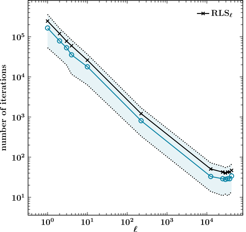
(b) $n=50\,000$

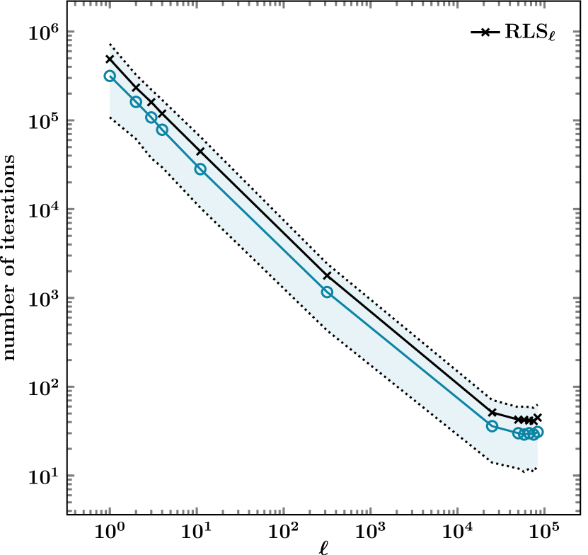
(c) $n=100\,000$

Figure 5: The empirical run time (number of iterations until an optimum was found) of RLS_ℓ on $\textsc{Majority}_{\lfloor\sqrt{n}\rfloor}$ for $n\in\{100,50\,000,100\,000\}$, each with varying values of $\ell$, as discussed at the beginning of Section IV-A. Note the doubly logarithmic scale. For each combination of $n$ and $\ell$, $1000$ independent runs with uniform initialization were started. The solid black line (points represented by $\times$) depicts the average of the runs. The solid blue line (points represented by $\circ$) depicts the median of the runs, and the surrounding shaded area depicts the range from the $25$th percentile to the $75$th percentile.

We complement our theoretical results on Majority with empirical investigations on a generalization of RLS called RLS_ℓ, which flips exactly $\ell$ bits each iteration. In more detail, RLS_ℓ follows Algorithm 2 and uses a time-homogeneous mutation operator, that is, it uses the same mutation operator in each iteration. Let $n\in\mathds{N}_{>0}$, and let $\bm{x}\in\{0,1\}^{n}$. Given an $\ell\in[n]$, for all $t\in\mathds{N}$, RLS_ℓ computes the result of $\phi_{t}(\bm{x})$ by first choosing a subset $I\subseteq[n]$ of cardinality $\ell$ uniformly at random among all $\ell$-size subsets of $[n]$ and then flipping exactly the bits at the positions in $I$. Note that RLS is a special case of RLS_ℓ for $\ell=1$.

In our experiments, we analyze the impact of the parameter $\ell$ of RLS_ℓ on the run time for Majority when using the uniform distribution as initialization distribution. To this end, given a problem size of $n\in\mathds{N}_{>0}$, with even $n$, we fix the parameter $r$ of $\textsc{Majority}_{r}$ to $\lfloor\sqrt{n}\rfloor$. Recalling our discussion of $r$ after Theorem 7, this results in an expected run time linear in $n$ for $\textsc{HasMajority}_{r}$, which is a lower bound for the run time for Majority (see Corollary 9). For larger values of $r$, the expected run time increases drastically. Thus, $r=\lfloor\sqrt{n}\rfloor$ results in an easily-solvable problem that is not yet trivial. We note though that, due to the uniform initialization, there is a constant probability of the initial solution being already optimal.

IV-A Near-optimal Value of $\ell$

We determine the value $\ell$ of RLS_ℓ that has the best average empirical run time among a variety of different values of $\ell$. For each each problem size $n\in\{10^{i}\mid i\in[2..5]\}\cup\{5\cdot 10^{i}\mid i\in[2..4]\}$, we consider $\ell\in\{1,2,3,4,\lfloor\ln n\rfloor,\lfloor\sqrt{n}\rfloor\}\cup\{\lfloor an/12\rfloor\mid a\in\{3\}\cup[6..10]\}$. For each parameter combination of $n$ and $\ell$, we start $1000$ independent runs of RLS_ℓ (on $\textsc{Majority}_{\lfloor\sqrt{n}\rfloor}$) and store its empirical run time, that is, the number of iterations $t$ from Algorithm 2 until an optimal solution was found for the first time. Afterward, we compute the average, median, and the $25$th as well as $75$th percentile. Figure 5 shows the results for $n\in\{100,50\,000,100\,000\}$.

The results for our values of $n$ look qualitatively similarly, that is, the run time drastically decreases by several orders of magnitude with increasing $\ell$ until $\ell\in\Theta\mathopen{}\mathclose{{}\left({n}}\right)$. The median is always below the mean, and the area between the $25$th percentile and the mean is larger than the one between the mean and the $75$th percentile. This is likely due to the initialization creating an optimal solution or one that is close to an optimal one with respect to its number of $1$s. Such runs result in a low run time. The mean being larger than the median suggests that initial solutions that are further away from optimal solutions in terms of their number of $1$s result in a far larger run time.

In the regime of $\ell\in\{\lfloor an/12\rfloor\mid a\in\{3\}\cup[6..10]\}$, the minimum average empirical run time is always taken for one of the values $\ell\in\{\lfloor an/12\rfloor\mid a\in[6..9]\}$. For these values of $\ell$, the difference of the smallest average to the second smallest is typically less than $1$. This suggests that, in this regime, the run time of RLS_ℓ does not dependent heavily on $\ell$. However, overall, a linear dependence of $\ell$ on $n$ seems best.

IV-B Trajectories for Different Values of $\ell$

The results in Figure 5 show that the value of $\ell$ has a drastic impact on the run time of RLS_ℓ on $\textsc{Majority}_{\lfloor\sqrt{n}\rfloor}$. Since $\ell$ only influences how largely the mutation changes the current solution but does not influence the selection of which solution to use for the next iteration, we compare the trajectories of RLS_ℓ for different values of $\ell$. We choose $n=10\,000$ and $\ell\in\{1,\lfloor\ln n\rfloor,\lfloor n/2\rfloor\}$, and we log at each iteration the number of $1$s of the currently best solution (the fitness level). Note that all optimal solutions are at fitness levels at least $5100$.

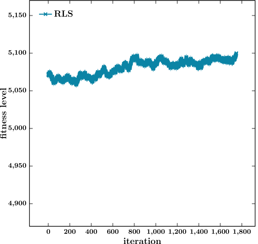
(a) $\ell=1$

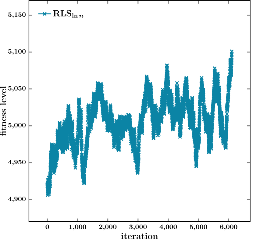
(b) $\ell=\lfloor\ln n\rfloor$

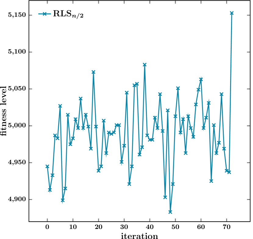
(c) $\ell=\lfloor n/2\rfloor$

Figure 6: The number of $1$s (fitness level) of the best solution of RLS_ℓ on $\textsc{Majority}_{\lfloor\sqrt{n}\rfloor}$ for $n=10\,000$ and for different values of $\ell$. Each plot depicts a single run that was stopped once an optimal solution was found (fitness level of at least $5100$). Note that we show runs that started from a non-optimal solution, chosen uniformly at random among all possible $2^{n}$ solutions.

Figure 6 depicts our results. Note that there is a huge difference in run time between $\ell=1$ and $\ell=\lfloor\ln n\rfloor$, which is most likely due to the former starting with a solution of more than $5000=n/2$ $1$s, whereas the latter starts at a position almost at $n/2-\sqrt{n}$. This highlights the impact of the initialization on the run time. Interestingly, the case $\ell=\lfloor n/2\rfloor$ also starts with a rather bad solution of about $n/2-\sqrt{n}/2$ $1$s but manages to quickly find an optimum. In fact, the last mutation increases the number of $1$s by about $200$. This suggests that RLS_ℓ has far better capabilities of exploring the plateau with $\ell\in\Theta\mathopen{}\mathclose{{}\left({n}}\right)$ than with smaller values of $\ell$.

V Conclusion

We analyzed the expected run time that RLS, started on a plateau, requires until it leaves the plateau for the first time. We considered a symmetric (HasMajority) and an asymmetric (Majority) setting, and we showed, for general EAs, how to derive a result for Majority from a result on HasMajority (Corollary 9), based on a more general result for a random process to reach a certain offset (Theorem 8). A fair amount of conditions of Corollary 9 follow directly from Lemmas 10 and 11, which apply to many EAs. Lemma 11 is so general that it holds for any EA that has, for each individual, a positive probability generating it. And although Lemma 10 is not as easy to check, we note that it holds for the $(1+1)~{}\textrm{EA}$ [21, Lemma $6.1$].

Theorem 8 provides a tool for analyzing general plateaus by considering phases in which the algorithm tries to cross the plateau. In order to bound the expected number of restarts, one determines the probability of crossing the plateau and not returning to its start. This can be done by defining a drift potential that decreases toward the end of the plateau (as done in the proof of Theorem 6) but is also $0$ at the start. The optional-stopping theorem allows then to determine the desired probability. However, we note that simply using the potential from the proof of Theorem 6 is typically a too coarse estimate since the bound always assumes the worst case of crossing the plateau. It remains an interesting open problem to derive tighter bounds for such a setting.

Further possible future work includes deriving a lower bound for RLS on HasMajority, as well as analyzing the expected run time of more algorithms on HasMajority, such as the $(1+1)~{}\textrm{EA}$, RLS_ℓ, or non-elitist EAs. Any such bound translates almost directly into a bound for Majority. Similarly, combining our results with those of Doerr et al. [2] on separable functions provides good bounds for RLS and the $(1+1)~{}\textrm{EA}$ on OneMax functions with any degree of neutrality from the W-model. Extending the results of Doerr et al. [2] to other algorithms or to functions other than OneMax also helps extend the picture about how well EAs cope with neutrality. Last, the current definitions of HasMajority and Majority let the algorithm either start on a plateau or in a global optimum. A potential generalization is to place the plateau somewhere else in the search space and introduce an easy slope toward the plateau. This follows the same idea as the function Plateau by Antipov and Doerr [5] but generalizing it even further such that the function has more than a single optimum.

Our long-term objective is to analyze the impact of the other components of the W-model problem generator proposed by Weise et al. [1] and extended by Doerr et al. [22]—first individually for each module (as done here for neutrality) and then for combinations of the four layers (neutrality, dummy variables, epistasis, and ruggedness). We see this as an important step towards run time results that more explicitly link algorithms’ performance to problem characteristics.

Carola Doerr, formerly Winzen, is since 2013 a permanent researcher at Sorbonne Unversité in Paris, France. Carola obtained her PhD in Computer Science from Saarland University and the Max Planck Institute for Informatics in 2011, and she successfully defender her habilitation (HDR) at Sorbonne Université in 2020. She works on theoretical analysis, benchmarking, and practical applications of black-box optimization heuristics.

Martin S. Krejca obtained his PhD from the Hasso Plattner Institute, University of Potsdam, Germany, in 2019. Since 2022, he is an assistant professor at Ecole Polytechnique, Palaiseau, France. His research interests are the theoretical analysis of random processes, especially black-box optimization heuristics.

References

• [1] T. Weise, Y. Chen, X. Li, and Z. Wu, “Selecting a diverse set of benchmark instances from a tunable model problem for black-box discrete optimization algorithms,” Applied Soft Computing, vol. 92, p. 106269, 2020.
• [2] B. Doerr, D. Sudholt, and C. Witt, “When do evolutionary algorithms optimize separable functions in parallel?” in Proc. of FOGA’13, 2013, pp. 51–64.
• [3] C. Bian, C. Qian, K. Tang, and Y. Yu, “Running time analysis of the (1+1)-EA for robust linear optimization,” Theoretical Computer Science, vol. 843, pp. 57–72, 2020.
• [4] J. Garnier, L. Kallel, and M. Schoenauer, “Rigorous hitting times for binary mutations,” Evol. Comput., vol. 7, no. 2, pp. 173–203, 1999.
• [5] D. Antipov and B. Doerr, “Precise runtime analysis for plateau functions,” ACM Trans. Evol. Learn. Optim., vol. 1, pp. 13:1–13:28, 2021.
• [6] H. Bambury, A. Bultel, and B. Doerr, “Generalized jump functions,” in Proc. of GECCO’21, 2021, pp. 1124–1132.
• [7] D. Antipov and S. Naumov, “The effect of non-symmetric fitness: the analysis of crossover-based algorithms on RealJump functions,” in Proc. of FOGA’21, 2021, pp. 10:1–10:15.
• [8] C. Witt, “On crossing fitness valleys with majority-vote crossover and estimation-of-distribution algorithms,” in Proc. of FOGA’21, 2021, pp. 2:1–2:15.
• [9] D.-C. Dang, T. Friedrich, T. Kötzing, M. S. Krejca, P. K. Lehre, P. S. Oliveto, D. Sudholt, and A. M. Sutton, “Escaping local optima with diversity mechanisms and crossover,” in Proc. of GECCO’16, 2016, pp. 645–652.
• [10] ——, “Escaping local optima using crossover with emergent diversity,” IEEE Transactions on Evolutionary Computation, vol. 22, no. 3, pp. 484–497, 2018.
• [11] L. D. Whitley, S. Varadarajan, R. Hirsch, and A. Mukhopadhyay, “Exploration and exploitation without mutation: Solving the jump function in \vartheta (n) time,” in Proc. of PPSN XV, 2018, pp. 55–66.
• [12] J. Lengler, “Drift analysis,” in [23].   Springer, 2020, pp. 89–131, also available at https://arxiv.org/abs/1712.00964.
• [13] J. He and X. Yao, “Drift analysis and average time complexity of evolutionary algorithms,” Artificial Intelligence, vol. 127, pp. 57–85, 2001.
• [14] B. Doerr, D. Johannsen, and C. Winzen, “Multiplicative drift analysis,” Algorithmica, vol. 64, no. 4, pp. 673–697, 2012.
• [15] T. Kötzing and M. S. Krejca, “First-hitting times under drift,” Theoretical Computer Science, vol. 796, pp. 51–69, 2019.
• [16] R. Durrett, Probability: theory and examples.   Cambridge University Press, 2019.
• [17] Y. Kovchegov. Mth 664: Lectures 24 - 27. Accessed 2021-10-28. [Online]. Available: http://sites.science.oregonstate.edu/~kovchegy/math664winter2013/664_lectures24-27.pdf
• [18] T. H. Cormen, C. E. Leiserson, R. L. Rivest, and C. Stein, Introduction to Algorithms, 3rd ed.   MIT Press, 2009.
• [19] T. Friedrich, A. Göbel, N. Klodt, M. S. Krejca, and M. Pappik, “Analysis of the survival time of the SIS and SIRS process on stars and cliques,” CoRR, vol. abs/2205.02653, 2022. [Online]. Available: http://arxiv.org/abs/2205.02653
• [20] B. Doerr, “Probabilistic tools for the analysis of randomized optimization heuristics,” in [23].   Springer, 2020, pp. 1–87, also available at https://arxiv.org/abs/1801.06733.
• [21] C. Witt, “Tight bounds on the optimization time of a randomized search heuristic on linear functions,” Combinatorics, Probability and Computing, vol. 22, no. 2, pp. 294–318, 2013.
• [22] C. Doerr, F. Ye, N. Horesh, H. Wang, O. M. Shir, and T. Bäck, “Benchmarking discrete optimization heuristics with iohprofiler,” Applied Soft Computing, vol. 88, p. 106027, 2020.
• [23] B. Doerr and F. Neumann, Eds., Theory of Evolutionary Computation: Recent Developments in Discrete Optimization, 1st ed.   Springer, 2020.