Conductivity of Two-dimensional Dirac Electrons Close to Merging in Organic Conductor $\alpha$-STF₂I₃ at Ambient Pressure

Abstract

The electric conductivity of Dirac electrons in the organic conductor $\alpha$-STF₂I₃ (STF = bis(ethylenedithio)diselenadithiafulvalene), which has an isostructure of $\alpha$-(BEDT-TTF)₂I₃, has been theoretically studied using a two-dimensional tight-binding model in the presence of both impurity and electron–phonon (e–p) scatterings. In contrast to $\alpha$-(BEDT-TTF)₂I₃, which has a Dirac cone with almost isotropic velocity, $\alpha$-STF₂I₃ provides a large anisotropy owing to a Dirac point that is close to merging. As a result, $\sigma_{x}$ becomes much larger than $\sigma_{y}$, where $\sigma_{y}$ and $\sigma_{x}$ are diagonal conductivities parallel and perpendicular to a stacking axis of molecules, respectively. With increasing temperature ($T$), $\sigma_{x}$ takes a broad maximum because of e–p scattering and $\sigma_{y}$ remains almost constant. The ratio $\sigma_{x}/\sigma_{y}$ is analyzed in terms of the band structure. Such an exotic conductivity of $\alpha$-STF₂I₃ is compared with that of an experiment showing a good correspondence. Finally, $\sigma_{x}/\sigma_{y}$ values of $\alpha$-ET₂I₃ and $\alpha$-BETS₂I₃ are shown to demonstrate the dissimilarity with $\alpha$-STF₂I₃.

1 Introduction

Since the discovery of two-dimensional massless Dirac fermions, [1] extensive studies have been explored in relevant materials. In particular, Dirac electrons have been found in the organic conductor [2, 3] $\alpha$-(BEDT-TTF)₂I₃  (BEDT-TTF=bis(ethylenedithio)tetrathiafulvalene) under uniaxial pressures. Using a tight-binding (TB) model, where transfer energies are estimated by the extended Hückel method,  [4, 5] we found that the density of states (DOS) vanishes linearly at the Fermi energy, [6] and the two-dimensional Dirac cone gives a zero-gap state (ZGS). [2] Such a Dirac cone was verified by first-principles DFT calculation, [7] which has been utilized for studying the electronic properties of $\alpha$-(BEDT-TTF)₂I₃  under hydrostatic pressures.[8]

There are several salts with an isostructure in organic conductors, [9, 10] $\alpha$-D₂I₃ (D = ET, STF, and BETS), where ET = BEDT-TTF; STF = bis(ethylenedithio)diselenadithiafulvalene, and BETS = bis(ethylenedithio)tetraselenafulvalene. These salts show an energy band with a Dirac cone [2, 11, 12, 13, 14, 15] and a nearly constant resistivity at high temperatures.[9, 10, 16, 17, 18, 19, 20]

The conductivity (or resistivity) of Dirac electrons has been studied theoretically using a two-band model with the conduction and valence bands. For a zero-doping, the static conductivity in the limit of absolute zero temperature remains finite with a universal value owing to a quantum effect.[21] The tilting of the Dirac cone provides the anisotropic conductivity, which results in the deviation of the current from the applied electric field. [22] At finite temperatures ($T$), the conductivity remains unchanged for $T<\Gamma$, where $\Gamma$ corresponds to the inverse of the lifetime determined from the impurity scattering. On the other hand, for $\Gamma\ll T$ the conductivity increases in proportion to $T$.[23] Since $\Gamma\sim$ 0.0003 eV for organic conductors,[3] a monotonic increase in the conductivity at high temperature ($T>0.0005$ eV) is theoretically expected. However, the measurement of the resistivity on the organic conductor shows an almost constant behavior at high temperatures. As a possible mechanism for such an exotic phenomenon, acoustic phonon scatterings have been proposed using the two-band model of the Dirac cone without tilting.  [24] Thus, it is necessary to clarify if such a mechanism reasonably explains the $T$ dependence of the conductivity of the actual organic conductor with the Dirac cone. In fact, the $T$ dependence of the conductivity in the presence of electron–phonon (e–p) scattering has been calculated for $\alpha$-ET₂I₃ [25] and $\alpha$-BETS₂I₃ [26]. As common features, they exhibit a small anisotropy at low temperatures and a nearly constant behavior at high temperatures. However, it is unclear if a similar behavior can be expected for $\alpha$-STF₂I₃, which contains disordered Se and S atoms with equal probabilities (50%:50%) for inner four chalcogen atoms [Fig. 1(a)]. Note that many of the STF salts exhibit electrical properties that indicate intermediate behavior between the isostructural ET and BETS salts, as if the solids do not contain any disorder but consist of a symmetrical donor containing imaginary atoms between selenium and sulfur at the inner chalcogen atoms[27, 28, 10, 29].

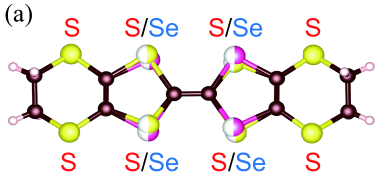
Figure 1: (Color online) (a) Molecular structure of STF, where STF = bis(ethylenedithio)diselenadithiafulvalene. The small and open circles designate carbon and hydrogen atoms, respectively. For sulfur (S) and selenium (Se), S/Se denotes that the site occupancy is given by S:Se = 50%:50%. [15] (b) TB model of $\alpha$-D₂I₃ (symbols) on the $x$–$y$ (crystallographic $b$–$a$) plane. A unit cell (dot-dashed line), which forms a square lattice, consists of four molecules A, A’, B, and C. The cross denotes an inversion center located in the middle of A and A’. The stacking direction corresponds to the $y$-axis (i.e., $a$-axis). Transfer energies between the nearest neighbor (NN) sites are shown by $g_{1},\cdots,h_{4}$.

In this paper, we examine the conductivity of $\alpha$-STF₂I₃ using a TB model with transfer energies, which are improved from a previous work. [15] The model [30] provides an electronic state with Dirac points close to merging, which has been theoretically shown in terms of the effective Hamiltonian.  [31, 32, 33] This paper is organized as follows. In Sect. 2, we briefly mention the difference in the estimation of transfer energies between our previous model [15] and the present one. [30] Our Hamiltonian consists of a TB model, impurity scattering, and e–p interaction with a reasonable coupling constant ($\lambda$) taken for an organic conductor. In Sect. 3, first, Dirac electrons are examined using the energy band and density of states. Next, the $T$ dependence of anisotropic conductivity, $\sigma_{x}$ ($\sigma_{y}$) being perpendicular (parallel) to the stacking axis, is calculated both in the absence and presence of e–p interaction. The ratio of $\sigma_{x}/\sigma_{y}$ is examined with several choices of $\lambda$. In Sect. 4, our calculation is compared with experimental results, [34, 35] by choosing a reasonable magnitude of $\lambda$. Section 5 is devoted to a summary and comparison of the $\sigma_{x}/\sigma_{y}$ of $\alpha$-STF₂I₃ with those of $\alpha$-ET₂I₃ and $\alpha$-BETS₂I₃.

2 Model and Formulation

2.1 Transfer energies of $\alpha$-STF₂I₃

Figure 1(a) shows the molecular structure and Fig. 1(b) shows the model describing crystal structures. The choice in the assignment of S or Se atoms for the inner chalcogen atoms in Fig. 1(a) produces randomness, which is given by the atom S/Se or Se/S around the central C=C bond, i.e., atoms on the left-hand side are given by S (pattern 1) or Se (pattern 2). The probabilities of these two patterns are exactly equal, forming a disordered crystal. In a previous model, [15] the transfer integral between nearest neighbor sites in Fig. 1(b) was calculated assuming statistically averaged structures between all the possible molecular arrangements coming from patterns 1 and 2. The present model was obtained by averaging the transfer energies of two extreme cases, which were deduced from the following consideration. [30] Note that single-crystal X-ray structural analyses revealed that all the inner four chalcogen atoms in Fig. 1(a) possess equal electron densities; [28, 35] thus, all the electron densities are obtained by averaging all the inner chalcogen atoms, suggesting a delocalized wave function. Instead of the previous localized wave functions of patterns 1 and 2, our new method provides a delocalized wave function, which is given by a linear combination of the patterns 1 and 2. [30] Such a delocalized wave function originates in a quantum interference between the two patterns. Expressing the wave function in terms of atomic orbitals and discarding the off-diagonal elements between S and Se, we obtain the following transfer energies. By rewriting the linear combination in terms of orbitals consisting of only S or Se, they are given by [30] $g_{1}$= 0.0535, $g_{2}$= 0.132, $g_{3}$= 0.0475, $h_{1}$=-0.0295, $h_{2}$= 0.295, $h_{3}$=0.1415, and $h_{4}$ =0.009.

2.2 Hamiltonian

We consider a two-dimensional Dirac electron system given by

$$H_{\rm total}=H_{0}+H_{\rm p}+H_{\rm e-p}+H_{imp}\;.$$ (1)

The spin is discarded. $H_{0}$ describes a TB model of $\alpha$-STF₂I₃ consisting of four molecules per unit cell (Fig. 1(b)). $H_{\rm p}$ and $H_{\rm e-p}$ denote an acoustic phonon and an e–p interaction, respectively. $H_{\rm imp}$ is the impurity potential. The terms $H_{0}+H_{\rm p}+H_{\rm e-p}$ provide the Fröhlich Hamiltonian [36] applied to the present Dirac electron system. The unit of energy is eV.

The TB Hamiltonian is expressed as

$$H_{0} = \sum_{i,j=1}^{N}\sum_{\alpha,\beta=1}^{4}t_{i,j;\alpha,\beta}a^{\dagger}_{i,\alpha}a_{j,\beta}$$ (2)

$$= \sum_{\bm{k}}\sum_{\alpha,\beta=1}^{4}t_{\alpha,\beta}(\bm{k})a^{\dagger}_{\alpha}(\bm{k})a_{\beta}(\bm{k})\;,$$

where $a^{\dagger}_{i,\alpha}$ denotes a creation operator of the electron with molecule $\alpha$ [ = A, A’, B, and C] at the $i$-th site. $a_{j}=1/N^{1/2}\sum_{\bm{k}}a_{\alpha}(\bm{k})\exp[i\bm{k}\cdot\bm{r}_{j}]$ with $\bm{k}=(k_{x},k_{y})$, and $N$ denotes the total number of lattices. The lattice constant is taken as unity. The transfer energies $t_{i,j;\alpha,\beta}$ are expressed in terms of $g_{1},\cdots,h_{4}$. The matrix elements $t_{\alpha,\beta}(\bm{k})$ $(\alpha,\beta=1,\cdots 4)$ in Eq. (2) are given by $t_{12}(\bm{k})=g_{3}+g_{2}Y$, $t_{13}(\bm{k})=h_{3}+h_{2}X$, $t_{14}(\bm{k})=h_{4}Y+h_{1}XY$, $t_{23}(\bm{k})=h_{2}+h_{3}X$, $t_{24}(\bm{k})=h_{1}+h_{4}X$, $t_{34}(\bm{k})=g_{1}+g_{1}Y$, and $t_{ij}(\bm{k})=t_{ji}^{*}(\bm{k})$ with $t_{ii}(\bm{k})=0$, where $X=\exp[ik_{x}]$ and $Y=\exp[ik_{y}]$.

Equation (2) is diagonalized as

$$\sum_{\beta=1}^{4}t_{\alpha,\beta}(\bm{k})d_{\beta\gamma(\bm{k})} = E_{\gamma}(\bm{k})d_{\alpha\gamma}(\bm{k})\;,$$ (3)

where $E_{1}(\bm{k})>E_{2}(\bm{k})>E_{3}(\bm{k})>E_{4}(\bm{k})$. The Dirac point ($\bm{k}_{\rm D}$) is calculated from

$$E_{1}(\bm{k}_{\rm D})=E_{2}(\bm{k}_{\rm D})=\epsilon_{\rm D}\;.$$ (4)

The ZGS is obtained when $\epsilon_{\rm D}$ becomes equal to the chemical potential at $T$=0.

The chemical potential $\mu$ is determined under the three-quarter-filled condition, which is given by

$$\frac{1}{N}\sum_{\bm{k}}\sum_{\gamma=1}^{4}f(E_{\gamma}(\bm{k})-\mu)$$

$$=\int_{-\infty}^{\infty}{\rm d}\omega D(\omega)f(\omega-\mu)=3\;,$$ (5)

where $f(\epsilon)=1/(\exp[\epsilon/T]+1)$ with $T$ being temperature in eV and $k_{\rm B}=1$ and

$$D(\omega) = \frac{1}{N}\sum_{\bm{k}}\sum_{\gamma}\delta(\omega-E_{\gamma}(\bm{k}))\;.$$ (6)

$D(\omega)$ denotes the density of states (DOS) per unit cell, which satisfies $\int{\rm d}\omega D(\omega)=4$.

In Eq. (1), the third term denotes the harmonic phonon given by $H_{\rm p}=\sum_{\bm{q}}\omega_{\bm{q}}b_{\bm{q}}^{\dagger}b_{\bm{q}}$ with $\omega_{\bm{q}}=v_{s}|\bm{q}|$ and $\hbar$ =1, whereas the fourth term is the e–p interaction expressed as [36]

$$H_{\rm e-p}=\sum_{\bm{k},\gamma}\sum_{\bm{q}}\alpha_{\bm{q}}c_{\gamma}(\bm{k}+\bm{q})^{\dagger}c_{\gamma}(\bm{k})\phi_{\bm{q}}\;,$$ (7)

with $\phi_{\bm{q}}=b_{\bm{q}}+b_{-\bm{q}}^{\dagger}$. The e–p scattering is considered within the same band (i.e., intraband) due to the energy conservation with $v\gg v_{s}$, where $v\simeq 0.05$ [8] denotes the average velocity of the Dirac cone. The last term of Eq. (1), $H_{\rm imp}$, denotes a normal impurity scattering, which gives a finite conductivity at low temperatures.

2.3 Conductivity

To study the anisotropic conductivity with damping by the impurity and e–p scatterings, we apply the following formula obtained from the linear response theory. Using $d_{\alpha\gamma}$ in Eq. (3), we calculate the conductivity per spin and per site as[37]

$$\sigma_{\nu\nu^{\prime}}(T) = \frac{e^{2}}{\pi\hbar N}\sum_{\bm{k}}\sum_{\gamma,\gamma^{\prime}=1}^{4}v^{\nu}_{\gamma\gamma^{\prime}}(\bm{k})^{*}v^{\nu^{\prime}}_{\gamma^{\prime}\gamma}(\bm{k})$$

$$\int_{-\infty}^{\infty}d\epsilon\left(-\frac{\partial f(\epsilon)}{\partial\epsilon}\right)$$

$$\times \frac{\Gamma_{\gamma}}{(\epsilon-\xi_{\gamma,\bm{k}})^{2}+\Gamma_{\gamma}^{2}}\times\frac{\Gamma_{\gamma^{\prime}}}{(\epsilon-\xi_{\gamma^{\prime},\bm{k}})^{2}+\Gamma_{\gamma^{\prime}}^{2}}\;,$$

$$v^{\nu}_{\gamma\gamma^{\prime}}(\bm{k}) = \sum_{\alpha,\beta}d_{\alpha\gamma}(\bm{k})^{*}\frac{\partial\tilde{H}_{\alpha\beta}}{\partial k_{\nu}}d_{\beta\gamma^{\prime}}(\bm{k})\;.$$ (9)

$\xi_{\gamma,\bm{k}}=E_{\gamma}(\bm{k})-\mu.$ $\nu=x$ and $y$. $h=2\pi\hbar$ and $e$ denote Planck’s constant and electric charge, respectively. The quantity $\Gamma_{\gamma}$ denotes the damping of the electron of the $\gamma$ band given by

$$\Gamma_{\gamma}=\Gamma+\Gamma_{\rm ph}^{\gamma}\;,$$ (10)

where the first term comes from the impurity scattering and the second term corresponding to the phonon scattering is given by [24]

$$\Gamma_{\rm ph}^{\gamma} = \frac{25\lambda}{2\pi v_{x}v_{y}}\times T|\xi_{\gamma,\bm{k}}|$$ (11a)

$$= C_{0}R\times T|\xi_{\gamma,\bm{k}}|\;,$$

$$R = \frac{\lambda}{\lambda_{0}}\;.$$ (11b)

$\lambda$ is given by $\lambda=|\alpha_{\bm{q}}|^{2}/\omega_{\bm{q}}$ and becomes independent of $|\bm{q}|$ for small $|\bm{q}|$. $v_{x}$ ($v_{y}$) denotes the velocity of the Dirac cone along the $x$ ($y$) axis. Since the estimation of $\lambda$ is complicated for organic conductors, we use an experimentally and theoretically deduced value $\lambda_{0}$ for one-dimensional conductor TCNQ salts, which gives $\lambda_{\rm 0}N(0)\sim 0.4$. [38, 39] The quantity $N(0)$ is the density of states given by $2/\pi v_{\rm F}$. For simplicity, the Fermi velocity $v_{\rm F}$ is replaced by the average velocity $(v_{x}v_{y})^{1/2}=v$. In the present calculation, we take $\lambda_{0}/2\pi v=0.1$, which is the same order as that of TCNQ. Thus, we introduce $R=\lambda/\lambda_{\rm 0}$ instead of $\lambda$, where $C_{0}=25\lambda_{\rm 0}/(2\pi v^{2})\simeq$ 50 (eV)^-1 with $v\simeq 0.05$ [8]. Note that $R=1$ corresponds to $\lambda=\lambda_{\rm 0}$. Compared with Ref. Suzumura_PRB_2018, Eq. (11a) is multiplied by 4 owing to the freedom of spin and valley.

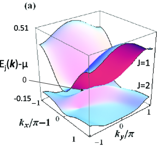
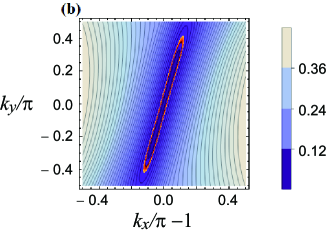
Figure 2: (Color online) (a) Conduction and valence bands given by $E_{1}(\bm{k})$ (upper band) and $E_{2}(\bm{k})$ (lower band), respectively, on the plane of $(k_{x}/\pi-1,k_{y})$, [30] measured from the chemical potential $\mu$=0.173. These two bands contact at Dirac points, $\bm{k}_{\rm D}/\pi-(1,0)=\pm(0.06,0.21)$ with an energy $\epsilon_{\rm D}$, which are obtained from $E_{1}(\bm{k}_{\rm D})=E_{2}(\bm{k}_{\rm D})=\epsilon_{\rm D}$. (b) Contour plots of $E_{1}(\bm{k})-E_{2}(\bm{k})$, where a scale is shown by a color bar. The yellow line denotes $E_{1}(\bm{k})-E_{2}(\bm{k})$ = 0.03, and the inside region represents the main contribution of the present calculation. The Dirac point $\pm\bm{k}_{\rm D}$ exists in the darkest region. (c) DOS as a function of $\omega-\mu$. The large peaks come from the van Hove singularity of the bands at time reversal invariant momonta (TRIMs) $E_{1}(\rm M)$ and $E_{2}(\rm Y)$, where M=$(\pi,\pi)$ and Y=$(0,\pi)$. Two peaks around $\omega-\mu=0$ correspond to the singularity at a TRIM X=$(\pi,0)$

3 Conductivity of $\alpha$-STF₂I₃  close to merging

3.1 Energy band

Dirac electrons close to the merging point are examined by calculating the energy band and DOS using Eq. (2). Figure 2(a) shows the conduction and valence bands, $E_{1}(\bm{k})$ and $E_{2}(\bm{k})$, respectively, measured from the chemical potential ($\mu$) on the plane of the 1st Brillouin zone. Note that the $k_{x}$ axis of the present choice [30] corresponds to $-k_{x}$ in Ref. Naito15 due to a different choice of a unit cell. These two bands contact at the Dirac points given by $\pm\bm{k}_{\rm D}=\pm(0.06,0.21)\pi$, which are close to a merging point given by a time reversal invariant momentum (TRIM) X [= $(\pi,0)$]. The origin of the energy is taken as the chemical potential of the 3/4-filled band. A pair of Dirac points are close to a merging point, X = $(\pi,0)$, since $E_{1}(\bm{k})-E_{2}(\bm{k})$ at $\bm{k}=(\pi,0)$ is much smaller than those at $\bm{k}=(0,\pi)$ and $(\pi,\pi)$. Figure 2(b) shows a contour plot of the energy difference $E_{1}(\bm{k})-E_{2}(\bm{k})$. The Dirac point is found at the darkest region inside the yellow line [$E_{1}(\bm{k})-E_{2}(\bm{k})=0.03$], which is elongated toward the X point. The contour close to the Dirac point shows the ellipse, where the ratio of the major axis to the minor axis is $\sim 12$ and the major axis is declined clockwise from the $k_{y}$ axis by an angle $\simeq\cos^{-1}(0.96)$. Note that the Dirac point is close to merging at the X point (TRIM), since the contour shows the ellipse elongated in the direction toward the X point and the velocity in this direction is much reduced.  [31, 32, 33] In Fig. 2(c), we show DOS corresponding to Fig. 2(a), which is obtained from the conduction ($E_{1}$) and valence ($E_{2}$) bands. The energy region relevant to the conductivity at low temperatures is within the interval range between two small peaks around $\omega-\mu=0$. In this region, DOS exhibits a linear dependence because of a Dirac cone. The cusp comes from an anomaly at $E_{1}(\rm X)$ and $E_{2}(\rm X)$

3.2 Anisotropic conductivity

We study the anisotropic conductivity by focusing on the diagonal $\sigma_{x}(=\sigma_{xx})$ and $\sigma_{y}(=\sigma_{yy})$ (i.e., $\sigma_{xy}<0$ is not shown) for the comparison with the experimental results. The conductivity calculated from Eq. (LABEL:eq:sigma) is normalized by $e^{2}/\hbar$. Impurity scattering is taken as $\Gamma$ = 0.0005. [25, 26]

Figure 3: $T$ dependence of conductivity $\sigma_{x}$ and $\sigma_{y}$ for $R$=0 (dotted line) and 0.5 (solid line), where $\Gamma$ = 0.0005. The inset shows the $T$ dependence of the chemical potential.

We examine the conductivity $\sigma_{x}$, which exhibits a dominant contribution to the conductivity. As shown later, the conductivity shows a large anisotropy, i.e., $\sigma_{y}\ll\sigma_{x}$, owing to the large anisotropy of the velocity of the Dirac cone. [22] Figure 3 shows the $T$ dependence of the conductivity $\sigma_{x}$ for R=0 and 0.5, where $R=0.5$ is a suitable choice of the e–p coupling constant. The $R$ dependence of $\sigma_{x}$ is also examined in Fig. 4. The inset of Fig. 3 denotes the corresponding chemical potential $\mu$, which is calculated from Eq. (5). $\mu$ decreases slightly at low temperatures but increases with increasing $T$ due to DOS, where a peak of the valence band ($E_{2}$) is larger than that of the conduction band ($E_{1}$).

First, we show the $T$ dependence of the conductivity for $R=0$. The conductivity of a simple Dirac cone with the isotropic and linear dispersion increases linearly with respect to $T$ owing to the linear increase in DOS. [24] A monotonic increase in the conductivity is also found for the energy band of the actual organic conductor with anisotropic velocity, although a slight deviation of the linear increase exists.  [25, 26] Since the conductivity remains constant at low temperatures, the transport of the Dirac electrons is well understood by the impurity scattering. However another scattering is needed to understand the almost constant behavior of $\sigma_{x}$ with increasing temperature.[24]

We next show the effect of e–p scattering on $\sigma_{\nu}$ ($\nu=x$ and $y$) using $R=0.5$. Compared with $\sigma_{\nu}$ with $R$ = 0, the conductivity for $R\not=0$ at high temperatures is noticeably reduced owing to the increase in $\Gamma_{\rm ph}^{\gamma}$ in the denominator of Eq. (LABEL:eq:sigma). It turns out that $\sigma_{x}$ shows a broad peak but $\sigma_{y}$ shows an almost constant behavior. With increasing $R$, $\sigma_{x}$ decreases noticeably at high temperatures ($0.08<T$), whereas the decrease in $\sigma_{y}$ is small. Note that such a large reduction in $\sigma_{x}$ by $R$ comes from $\sigma_{x}$ being much larger than $\sigma_{y}$, which magnifies the behavior of $\sigma_{x}$ on a visible scale. The large anisotropy of the conductivity originates from the anisotropy of the velocity $v_{x}$ being larger than $v_{y}$, since $\sigma_{x}\propto v_{x}/v_{y}$ and $\sigma_{y}\propto v_{y}/v_{x}$. [22] As shown in Figs. 2(a) and 2(b), the large anisotropy of the velocity is a characteristic of the Dirac cone close to merging. The difference in $\sigma_{\nu}$ between $R$ = 0 and 0.5 becomes negligibly small for $T<0.003$, since the e–p interaction becomes ineffective at low temperatures.

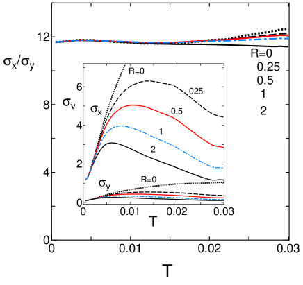
Figure 4: (Color online) $T$ dependence of $\sigma_{x}/\sigma_{y}$ for several choices of e–p coupling; $R$=0 (dotted line), 0.25 (dashed line), 0.5 (solid line), 1 (dot-dashed line), and 2 (solid line), where $\Gamma$ = 0.0005. The inset shows the $T$ dependence of the corresponding $\sigma_{x}$ and $\sigma_{y}$.

The conductivity of $\sigma_{\nu}(T)$ for $R$ = 0, 0.25, 0.5, 1, and 2 is shown in the inset of Fig. 4. With increasing $R(\propto\lambda)$, $\sigma_{\nu}$ with a fixed $T$ decreases rapidly owing to the increase of the e–p interaction ($\lambda$), which appears in the denominator of Eq. (LABEL:eq:sigma). Since $\Gamma_{\rm ph}^{\gamma}\propto\lambda T$, the peak of $\sigma_{x}$ at $T=T_{\rm max}$ decreases and $T_{\rm max}$ also decreases.

In Fig. 4, the $T$ dependence of $\sigma_{x}/\sigma_{y}$ is shown to comprehend an anisotropy of the conductivity. At low temperatures, $\sigma_{x}/\sigma_{y}(\simeq 12)$ is almost independent of $T$ and $R$. At high temperatures ($0.02<T$), $\sigma_{x}/\sigma_{y}$ for $R=0$, 0.25, 0.5, and 1 (2) increases (decreases) slightly. Such behavior of $\sigma_{x}/\sigma_{y}$ with respect to $T$ suggests that $\sigma_{x}/\sigma_{y}$ is determined by $v_{x}/v_{y}$ but is almost independent of the scattering by impurities and phonons. Here, we analyze $\sigma_{x}/\sigma_{y}$ using Fig. 2(b). The contour of $E_{1}(\bm{k})-E_{2}(\bm{k})$ encircling the Dirac point shows the ellipse with a focus at the Dirac point, and the axis rotated clockwise from the $k_{y}$ axis with an angle $\theta$. The principal values of the conductivity, $\sigma_{+}$ and $\sigma_{-}$, show $\sigma_{+}/\sigma_{-}\simeq(v_{+}/v_{-})^{2}$. $v_{+}$ and $v_{-}$ are velocities of the Dirac cone corresponding to the minor axis and the major axis of the ellipse, respectively. [22] In terms of $\theta$, $\sigma_{+}$, and $\sigma_{-}$, the ratio of $\sigma_{x}$ to $\sigma_{y}$ is given by

$$\frac{\sigma_{x}}{\sigma_{y}} = \frac{(\sigma_{+}/\sigma_{-})^{2}+\tan^{2}\theta}{(\sigma_{+}/\sigma_{-})^{2}\tan^{2}\theta+1}\;.$$ (12)

Substituting $\sigma_{+}/\sigma_{-}\simeq 12$ and $\tan\theta\simeq 0.28$ into Eq. (12), we obtain $\sigma_{x}/\sigma_{y}\simeq 11.7$, which is almost equal to the numerical value in Fig. 4. Note that $\sigma_{x}/\sigma_{y}$ is mainly determined by $\theta$ for large $\sigma_{+}/\sigma_{-}$, i.e., for the case of an extremely elongated ellipse.

4 Comparison with Experiment

Figure 5: (Color online) Theoretical results (lines) and those of experiment (symbols), [34] where $\sigma_{x}$ ($\sigma_{y}$) corresponds to $\sigma_{b}^{\rm exp}$ ($\sigma_{a}^{\rm exp}$). $\sigma_{x}$ and $\sigma_{y}$ are compared with $\sigma_{b}^{\rm exp}$ and $\sigma_{a}^{\rm exp}$, respectively.

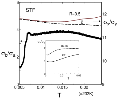
Figure 6: $T$ dependence of $\sigma_{b}^{\rm exp}/\sigma_{a}^{\rm exp}$ (symbols) from Ref. Naito2020b and $\sigma_{x}/\sigma_{y}$ from the present calculation with $R$ = 0.5 (solid line) and 2 (dashed line). The inset is discussed in Sect. 5, where $\sigma_{x}/\sigma_{y}$ values for ET ($R$=0.5) and BETS ($R$=1) were obtained from Refs. Suzumura2021 and Suzumura2021b, respectively.

Finally, we compare the present theoretical result with that of the experiment, [34] where $\sigma_{b}^{\rm exp}$ and $\sigma_{a}^{\rm exp}$ (symbols) correspond to $\sigma_{x}$ and $\sigma_{y}$, respectively. In Fig. 5, $\sigma_{x}$ and $\sigma_{y}$ are compared with $\sigma_{b}^{\rm exp}$ and $\sigma_{a}^{\rm exp}$. The experimental (theoretical) result is shown using the left (right) axis. The e–p coupling constant $\lambda$ is taken as $R$=0.5 to obtain $T_{\rm max}$ of $\sigma_{x}$ equal to that of $\sigma_{b}^{\rm exp}$, where the conductivity becomes maximum at $T$ = $T_{\rm max}$. The scale of $\sigma_{x}$ is taken such that the maximum $\sigma_{b}^{\rm exp}$ becomes equal to the maximum $\sigma_{x}$. A good coincidence between $\sigma_{b}^{\rm exp}$ and $\sigma_{x}$ is obtained in the region of $0.006<T<0.024$. Moreover, a comparison of $\sigma_{a}^{\rm exp}$ and $\sigma_{y}$ gives $\sigma_{a}^{\rm exp}\simeq 4\sigma_{y}$ for $0.008<T$, where both show nearly constant behaviors. The rapid decrease in both $\sigma_{b}^{\rm exp}$ and $\sigma_{a}^{\rm exp}$ for $T\simeq 0.006$ suggests the reduction of the Fermi surface. In fact, the $T$ dependence of the resistivity of $\alpha$-STF₂I₃ shows a behavior between those of $\alpha$-ET₂I₃ and $\alpha$-BETS₂I₃, [28, 10] where the former becomes the insulating state due to charge ordering [3] and the latter remains in a metallic state. [13, 14] Thus, the reduction of the conductivity at low temperature may be ascribed to the charge fluctuation. Namely, the comparison of the present TB model with the experiment may be justified for $0.006<T$.

In Fig. 6, the $T$ dependence of $\sigma_{x}/\sigma_{y}$ ($R$=0.5) is compared with that of $\sigma_{b}^{\rm exp}/\sigma_{a}^{\rm exp}$. The temperature variations of $\sigma_{x}/\sigma_{y}$ for $0.005<T$ and $\sigma_{b}^{\rm exp}/\sigma_{a}^{\rm exp}$ for $0.008<T$ are small. At higher temperatures, $\sigma_{x}/\sigma_{y}$ shows a slight increase (decrease) for $R$ = 0.5 ($R$=2), whereas $\sigma_{b}^{\rm exp}/\sigma_{a}^{\rm exp}$ decreases. The broad maximum of $\sigma_{b}^{\rm exp}/\sigma_{a}^{\rm exp}$ around $T\simeq$ 0.015 comes from the fact that $\sigma_{b}^{\rm exp}$ takes a broad maximum at $T\simeq 0.012$, whereas $\sigma_{a}^{\rm exp}$ for $0.01<T$ decreases linearly and slowly. The almost constant behavior of $\sigma_{x}/\sigma_{y}$ suggesting the same $T$ dependence is understood from the magnified scale of $\sigma_{x}$ and $\sigma_{y}$, which show a common behavior of a broad maximum at $T\simeq 0.01$. However, the linear dependence in $\sigma_{a}^{\rm exp}$ is not yet clear and a further consideration beyond Eq. (11a) may be needed.

5 Summary and Discussion

In summary, we examined the $T$ dependence of the conductivity of Dirac electrons in the organic conductor $\alpha$-STF₂I₃ at ambient pressure. A large anisotropy, which comes from the Dirac point close to merging, gives rise to the characteristics of $\sigma_{\nu}$, where $\sigma_{x}$ takes a broad maximum owing to e–p scattering with increasing temperature. The ratio of $\sigma_{x}/\sigma_{y}$ is almost independent of $T$ owing to the large anisotropy of the velocity and the axes of the ellipse rotated from the $k_{y}$ and $k_{x}$ directions. We compared the conductivity in the present calculation with that in the experiment. To our best knowledge, this is the first experimental demonstration of the $T$ dependence of the anisotropic conductivity in organic Dirac electrons. The experimental result of $\alpha$-STF₂I₃ was reasonably explained by the present calculation of the TB model with e–p interaction. It will be interesting to examine the current deviation from the electric field due to $\sigma_{xy}\not=0$.

Here, we compare the present $\sigma_{x}/\sigma_{y}$ of $\alpha$-STF₂I₃ (Fig. 4) with those of other organic conductors, $\alpha$-(BEDT-TTF)₂I₃  and $\alpha$-BETS₂I₃, which show band structures with almost isotropic velocities owing to Dirac points being away from TRIM. In the inset of Fig. 6, the $T$ dependences of $\sigma_{x}/\sigma_{y}$ for $\alpha$-(BEDT-TTF)₂I₃  and $\alpha$-BETS₂I₃ are shown, which display the visible increase with increasing $T$ in contrast to $\sigma_{x}/\sigma_{y}$ of $\alpha$-STF₂I₃. For ET (under hydropressures), [25] a small anisotropy of the velocity ($v_{x}/v_{y}\simeq 1.2$) shows $\sigma_{x}/\sigma_{y}\simeq 1.4$, which is compensated by the tilting of the Dirac cone ($\eta=v_{t}/V\simeq 0.8$ with $v_{t}$ and $V$ being the tilting and averaged velocities of the Dirac cone, respectively). As a result, $\sigma_{x}/\sigma_{y}\simeq 1$ at low temperatures and increases with increasing $T$. For BETS, [26] the anisotropy of the velocity ($v_{x}/v_{y}\simeq 1.4$) is slightly larger and dominates the effect of tilting ($\eta\simeq 0.8$). Therefore, anisotropic conductivity shows $\sigma_{x}/\sigma_{y}\simeq 1.4$ at low temperatures and increases to a finite value with increasing $T$. Note that $\sigma_{x}/\sigma_{y}$ of $\alpha$-ET₂I₃ and $\alpha$-BETS₂I₃ clearly increases with increasing $T$ owing to almost isotropic velocities. Thus, as shown in Eq. (12), the almost $T$-independent behavior of $\sigma_{x}/\sigma_{y}(\gg 1)$ in $\alpha$-STF₂I₃ is ascribed to the large anisotropy of the velocity ($v_{x}/v_{y}\gg 1$), which originates from the Dirac point close to merging.

- [1] K. S. Novoselov, A. K. Geim, S. V. Morozov, D. Jiang, M. I. Katsnelson, I. V. Grigorieva, S. V. Dubonos, and A. A. Firsov, Nature 438, 197 (2005).
- [2] S. Katayama, A. Kobayashi, and Y. Suzumura, J. Phys. Soc. Jpn. 75, 054705 (2006).
- [3] K. Kajita, Y. Nishio, N. Tajima, Y. Suzumura, and A. Kobayashi, J. Phys. Soc. Jpn. 83, 072002 (2014).
- [4] T. Mori, A. Kobayashi, Y. Sasaki, H. Kobayashi, G. Saito, and H. Inokuchi, Chem. Lett. 13, 957 (1984).
- [5] R. Kondo, S. Kagoshima, and J. Harada, Rev. Sci. Instrum. 76, 093902 (2005).
- [6] A. Kobayashi, S. Katayama, K. Noguchi, and Y. Suzumura, J. Phys. Soc. Jpn. 73, 3135 (2004).
- [7] H. Kino and T. Miyazaki, J. Phys. Soc. Jpn. 75, 034704 (2006).
- [8] S. Katayama, A. Kobayashi, and Y. Suzumura, Eur. Phys. J. B 67, 139 (2009).
- [9] M. Inokuchi, H. Tajima, A. Kobayashi, H. Kuroda, R. Kato, T. Naito, and H. Kobayashi, Synth. Met. 56, 2495 (1993).
- [10] M. Inokuchi, H. Tajima, A. Kobayashi, T. Ohta, H. Kuroda, R. Kato, T. Naito, and H. Kobayashi, Bull. Chem. Soc. Jpn. 68, 547 (1995)
- [11] R. Kondo, S. Kagoshima, N. Tajima, and R. Kato, J. Phys. Soc. Jpn. 78, 114714 (2009).
- [12] T. Morinari and Y. Suzumura, J. Phys. Soc. Jpn. 83, 094701 (2014).
- [13] S. Kitou, T. Tsumuraya, H. Sawahata, F. Ishii, K. Hiraki, T. Nakamura, N. Katayama, and H. Sawa, Phys. Rev. B 103, 035135 (2021).
- [14] T. Tsumuraya and Y. Suzumura, Eur. Phys. J. B 94, 17 (2021).
- [15] T. Naito, R. Doi, and Y. Suzumura, J. Phys. Soc. Jpn. 89, 023701 (2020).
- [16] K. Kajita, T. Ojiro, H. Fujii, Y. Nishio, H. Kobayashi, A. Kobayashi, and R. Kato, J. Phys. Soc. Jpn. 61, 23 (1992).
- [17] N. Tajima, M. Tamura, Y. Nishio, K. Kajita, and Y. Iye, J. Phys. Soc. Jpn. 69, 543 (2000).
- [18] N. Tajima, A. Ebina-Tajima, M. Tamura, Y. Nishio, and K. Kajita, J. Phys. Soc. Jpn. 71, 1832 (2002).
- [19] N. Tajima, S. Sugawara, M. Tamura, R. Kato, Y. Nishio, and K. Kajita, Europhys. Lett. 80, 47002 (2007).
- [20] D. Liu, K. Ishikawa, R. Takehara, K. Miyagawa, M. Tanuma, and K. Kanoda, Phys. Rev. Lett. 116, 226401 (2016).
- [21] N. H. Shon and T. Ando, J. Phys. Soc. Jpn. 67, 2421 (1998).
- [22] Y. Suzumura, I. Proskurin, and M. Ogata, J. Phys. Soc. Jpn. 83, 023701 (2014).
- [23] N. M. R. Peres, F. Guinea, and A. H. Castro Neto, Phys. Rev. B 73, 125411 (2006).
- [24] Y. Suzumura and M. Ogata, Phys. Rev. B 98, 161205 (2018).
- [25] Y. Suzumura and M. Ogata, J. Phys. Soc. Jpn. 90, 044709 (2021).
- [26] Y. Suzumura and T. Tsumuraya, J. Phys. Soc. Jpn. 90, 124707 (2021).
- [27] T. Naito, A. Miyamoto, H. Kobayashi, R. Kato, and A. Kobayashi, Chem. Lett. 21, 119 (1992).
- [28] T. Naito, Dr. Thesis, Graduate School of Science, The University of Tokyo, Tokyo (1995).
- [29] T. Naito, H. Kobayashi, and A. Kobayashi, Bull. Chem. Soc. Jpn. 70, 107 (1997).
- [30] T. Naito and Y. Suzumura, Crystals 12, 346 (2022).
- [31] G. Montambaux, F. Piechon, J. -N. Fuchs, and M. O. Goerbig, Eur. Phys. J. B 72, 509 (2009).
- [32] G. Montambaux, F. Piechon, J. -N. Fuchs, and M. O. Goerbig, Phys. Rev. B 80, 153412 (2009).
- [33] A. Kobayashi, Y. Suzumura, F. Piechon, and G. Montambaux, Phys. Rev. B 84, 075450 (2011).
- [34] T. Naito and R. Doi, Crystals 10, 270 (2020).
- [35] T. Naito, Crystals 11, 838 (2021).
- [36] H. Fröhlich, Proc. Phys. Soc. A223, 296 (1954).
- [37] S. Katayama, A. Kobayashi, and Y. Suzumura, J. Phys. Soc. Jpn. 75, 023708 (2006).
- [38] M. J. Rice, L. Pietronero, and P. Brüesh, Solid State Commun. 21, 757 (1977).
- [39] H. Gutfreund, C. Hartzstein, and M. Weger, Solid State Commun. 36, 647 (1980).