Analysis of lowest-order characteristics-mixed FEMs for incompressible miscible flow in porous media

Abstract

The time discrete scheme of characteristics type is especially effective for convection-dominated diffusion problems. The scheme has been used in various engineering areas with different approximations in spatial direction. The lowest-order mixed method is the most popular one for miscible flow in porous media. The method is based on a linear Lagrange approximation to the concentration and the zero-order Raviart-Thomas approximation to the pressure/velocity. However, the optimal error estimate for the lowest-order characteristics-mixed FEM has not been presented although numerous effort has been made in last several decades. In all previous works, only first-order accuracy in spatial direction was proved under certain time-step and mesh size restrictions. The main purpose of this paper is to establish optimal error estimates, $i.e.$, the second-order in $L^{2}$-norm for the concentration and the first-order for the pressure/velocity, while the concentration is more important physical component for the underlying model. For this purpose, an elliptic quasi-projection is introduced in our analysis to clean up the pollution of the numerical velocity through the nonlinear dispersion-diffusion tensor and the concentration-dependent viscosity. Moreover, the numerical pressure/velocity of the second-order accuracy can be obtained by re-solving the (elliptic) pressure equation at a given time level with a higher-order approximation. Numerical results are presented to confirm our theoretical analysis.

Key words: Modified method of characteristics, mixed finite element method, incompressible miscible flow.

1 Introduction

In many engineering areas, one often solves the following miscible displacement system modeling an incompressible flow in a porous medium $\Omega$

$$\Phi\frac{\partial c}{\partial t}-\nabla\cdot(D(\mathbf{u})\nabla c)+\mathbf{u}\cdot\nabla c=c_{1}q^{I}-cq^{P},$$ (1.1)

$$\nabla\cdot\mathbf{u}=q^{I}-q^{P},$$ (1.2)

$$\mathbf{u}=-\frac{k(x)}{\mu(c)}\nabla p,$$ (1.3)

for $t\in[0,T]$, with the initial condition

$$c(x,0)=c_{0}(x),\qquad\textrm{for }x\in\Omega,$$ (1.4)

where we assume that the domain $\Omega\in{\bf R}^{d}$, $d=2,3$, is bounded and the condition $\int_{\Omega}pdx=0$ is enforced for the uniqueness of the solution. In the above system, $c$ represents the concentration of one of the fluids, $\mathbf{u}$ the Darcy velocity and $p$ the pressure of the fluid mixture. $\Phi$ denotes the porosity of the medium, $q^{I}$ and $q^{P}$ are given injection and production sources, $c_{1}$ is the concentration of the first component in the injection source, $D(\mathbf{u})=[D_{ij}(\mathbf{u})]_{d\times d}$ is the diffusion-dispersion tensor (see [3] for details), $k(x)$ is the permeability of the medium and $\mu(c)$ is the concentration-dependent viscosity of the fluid mixture.

In the last several decades, numerical methods and analyses for the miscible displacement system (1.1)-(1.3) have been studied extensively, $e.g.$, see [19, 22, 37, 42] and references therein. Two review articles were written by Ewing and Wang [24] and Scovazzi et. al. [45], respectively. In particular, Ewing and Wheeler [25] proposed a fully discrete Galerkin-Galerkin finite element method for the miscible displacement problem in two dimensional space. Later, Douglas et al. [16] introduced a Galerkin-mixed finite element method for solving the system (1.1)-(1.3). In both [16] and [25], a linearized semi-implicit Euler scheme was applied for the time discretization, and a time step condition $\tau=o(h)$ was required to obtain optimal error estimates. Since the concentration equation (1.1) is often convection-dominated, $i.e.$, the diffusion coefficient $D$ is small in many applications, the characteristics time discretization is more effective for solving this system. A modified method of characteristics (MMOC) with both finite difference and finite element approximations was proposed by Douglas and Russell [17] for linear convection-dominated diffusion problems. The method is based on the backward Euler scheme in the characteristic time direction and classical Galerkin FE approximations in spatial direction. The method was extended to the nonlinear miscible displacement equations in [23] with a Galerkin-mixed approximation, where the error estimate

$$\|c^{n}-c_{h}^{n}\|_{L^{2}}+\|p^{n}-p_{h}^{n}\|_{L^{2}}+\|{\bf u}^{n}-{\bf u}_{h}^{n}\|_{H(div)}\leq C(\tau+h_{c}^{r+1}+h_{p}^{k+1})\,$$ (1.5)

was established for $d=2$ under the time step restriction $\tau=o(h_{p})$ and some mesh size conditions, where $D({\bf u})$ is assumed to be global Lipschitz satisfying

$$\frac{\partial D(x,{\bf v})}{\partial{\bf v}}\leq K^{*}$$ (1.6)

and $h_{c}$ and $h_{p}$ denotes the mesh size of the partition for the concentration equation and the pressure equation, respectively.

The most commonly-used Galerkin-mixed method in practical computation is the lowest order one (k = 0,r = 1) [9, 10, 16, 20, 25, 29, 45, 48]. For the lowest-order mixed method, the error estimate (1.5) reduces to

$$\|c^{n}-c_{h}^{n}\|_{L^{2}}+\|p^{n}-p_{h}^{n}\|_{L^{2}}+\|{\bf u}^{n}-{\bf u}_{h}^{n}\|_{H(div)}\leq C(\tau+h_{p}+h_{c}^{2})$$ (1.7)

under the more tightened restriction

$$\tau\leq O(h_{p}^{2})\,,$$ (1.8)

for $d=3$ (see (4.42) in [23]). Numerous effort has been devoted to weakening the time step restriction and mesh size condition [12, 20, 44, 47, 51]. Amongst them, Duran [20] showed the error estimate (1.5) under a weaker time-step restriction $\tau=o(h_{c})$ for $d=3$, the Lipschitz condition (1.6) for $D({\bf u})$ and $k\geq 1$. Analysis can be extended to the case $k=0$ as pointed out by the author. Further improvement was given recently in [51], where in terms of an error splitting technique the above error estimate was proved almost unconditionally, i.e., under the condition $\tau\leq o(1)$ and without the Lipschitz condition (1.6) for $D({\bf u})$. However, the analysis was limited to $k=r\geq 1$ which exclude the popular lowest-order mixed method. Moreover the modified method of characteristics combined with many other approximations in spatial direction has also been studied extensively [12, 14, 27, 32, 33, 38, 39, 47]. To maintain the conservation of the mass, a related Eulerian-Lagrangian localized adjoint method (ELLAM) was studied in [8, 49] for advective-diffusive equations, in which an ELLAM scheme was used in time direction. Analysis of an ELLAM-MFEM for (1.1)-(1.3) was presented in [49, 50]. A more general ELLAM scheme was proposed and investigated in the recent work [11]. The convergence rate of the method in spatial direction is similar to those in (1.5) and (1.7). Some other type methods of characteristics can be found in [2, 31, 40]. In addition, the characteristics type methods have been applied and analyzed for many other linear and nonlinear parabolic PDEs from various engineering applications [2, 4, 19, 27, 28, 38, 46]. Numerical simulations show that the time-truncation errors of the MMOC are much smaller than those of standard schemes for convection-dominated models.

There are still several issues to be further addressed for the popular lowest-order characteristics-mixed FEM. (i). In the lowest-order characteristics-mixed method, a linear Lagrange approximation and a zero-order Raviart-Thomas approximation are used for the concentration and the pressure/velocity, respectively. Clearly, the error estimate presented in (1.7) is not optimal for the concentration in $L^{2}$-norm, while the concentration is a more important physical component in practical applications. (ii). The modified method of characteristics is based on characteristic tracking, along which the method may greatly reduce the temporal error and allow one to use a large time step in computations. However, certain tightened time-step condition was always required in previous analysis. (iii). The Lipschitz condition (1.6) for the diffusion-disperson tensor $D({\bf u})$ may not be realistic in practice. Analysis of Galerkin-mixed FEMs for (1.1)-(1.3) under a weaker assumption of $D({\bf u})$ being smooth (without the global Lipschitz condition (1.6)) was done in [9, 16], which, however, leads to some more serious mesh condition for the lowest-order mixed method.

This paper focuses on a new analysis of the lowest-order characteristics-mixed finite element method for the nonlinear and coupled system (1.1)-(1.3). We shall establish the optimal $L^{2}$-norm error estimates

$$\|c^{n}-c_{h}^{n}\|_{L^{2}}\leq C(\tau+h^{2})$$ (1.9)

$$\|p^{n}-p_{h}^{n}\|_{L^{2}}+\|{\bf u}^{n}-{\bf u}_{h}^{n}\|_{H(div)}\leq C(\tau+h)$$ (1.10)

only under the condition

$$\tau=o\left(\frac{1}{|\log h|}\right)$$ (1.11)

and the weak assumption of $D({\bf u})$ being smooth (without the global Lipschitz condition (1.6)). The new analysis shows that the method provides a second-order accuracy for the concentration, while only first-order accuracy was proved in previous works. Moreover, with the numerical concentration of second-order accuracy, a second-order pressure/velocity at a given time level can be obtained by re-solving the elliptic pressure equation with a first-order RT approximation. The extension to more general cases with higher-order approximations and different mesh partitions can be made analogously. The analysis presented in this paper is based on an elliptic quasi-projection proposed in [48], an error splitting technique presented in [35] and negative-norm estimate of the numerical velocity. With the quasi-projection and some more precise estimates in the characteristic direction, the lower-order approximation to the pressure/velocity does not pollute the accuracy of numerical concentration in our analysis. The optimal analysis under the weaker time step condition (2.8) is given in terms of the error splitting technique.

The paper is organized as follows. In Section 2, we present our notations and our main results. A new re-covering technique is introduced, with which the second-order accuracy of numerical velocity/pressure can be obtained by re-solving the elliptic pressure equation with a higher-order approximation and the obtained numerical concentration. In section 3, we first present several useful lemmas and more precise estimates in the characteristic direction. In terms of the error splitting argument, we analyze the temporal and spatial errors, respectively and the boundedness of numerical solutions. Then, we present optimal error estimates of the numerical scheme. In Section 4, numerical results are given to confirm our theoretical analysis.

2 Main results

We at first define some notations used in this paper. For any integer $m\geq 0$ and $1\leq p\leq\infty$, let $W^{m,p}(\Omega)$ be the Sobolev space of functions with the norm

$$\|f\|_{W^{m,p}}=\left\{\begin{array}[]{ll}\Big{(}\displaystyle\sum\limits_{|\beta|\leq m}\int_{\Omega}|D^{\beta}f|^{p}dx\Big{)}^{\frac{1}{p}},&\textrm{for }1\leq p<\infty,\\ \displaystyle\sum\limits_{|\beta|\leq m}\textrm{ess}\sup_{\Omega}|D^{\beta}f|,&\textrm{for }p=\infty,\end{array}\right.$$

where

$$D^{\beta}=\frac{\partial^{|\beta|}}{\partial x_{1}^{\beta_{1}}\cdots\partial x_{d}^{\beta_{d}}},$$

for the multi-index $\beta=(\beta_{1},\cdots,\beta_{d})$, $\beta_{1}\geq 0,\cdots,\beta_{d}\geq 0$, and $|\beta|=\beta_{1}+\cdots+\beta_{d}$. When $p=2$, we denote $W^{m,2}(\Omega)$ by $H^{m}(\Omega)$. We define $L_{0}^{k}(\Omega)=\{f\in L^{k}(\Omega):\int_{\Omega}fdx=0\}$ and $H(\textrm{div};\Omega)=\{\mathbf{f}=(f_{1},\cdots,f_{d}):f_{i},\nabla\cdot\mathbf{f}\in L^{2}(\Omega),1\leq i\leq d\}$. For simiplicity, we write ${\bf f}\in W^{m,p}$ if $f_{i}\in W^{m,p}$. To avoid technical difficulties on boundary, we assume that $\Omega$ is a rectangle in $\mathbb{R}^{2}$ (or cuboid in $\mathbb{R}^{3}$) and the problem (1.1)-(1.3) and the corresponding FE spaces are $\Omega$-periodic as usual [23, 39, 44, 51].

Let $\pi_{h}$ be a quasi-uniform partition of $\Omega$ into triangles $T_{j}$, $j=1,\cdots,M$, in $\mathbb{R}^{2}$ (or tetrahedra in $\mathbb{R}^{3}$) of diameter less than $h$. We denote by $(S_{h}^{k},H_{h}^{k})$ $k$-order Raviart-Thomas finite element space [43]

$$S_{h}^{k}:=\{w\in L^{2}_{0}(\Omega):w|_{T_{j}}\in P_{k}\}$$

$$H_{h}^{k}:=\{{\bf v}\in H(\textrm{div};\Omega):{\bf v}|_{T_{j}}\in P_{k}\otimes xP_{k}\}$$

and by $V_{h}^{1}$ the standard linear Lagrange FE space on the partition $\pi_{h}$ where $P_{k}$ denotes the polynomial space of degree $\leq k$.

Let $\{t_{n}|t_{n}=n\tau;0\leq n\leq N\}$ be a uniform partition of $[0,T]$ with the time step $\tau=T/N$, and we denote

$$c^{n}(x)=c(x,t_{n}),\quad\mathbf{u}^{n}(x)=\mathbf{u}(x,t_{n}),\quad p^{n}(x)=p(x,t_{n}).$$

For a sequence of functions $\{\omega^{n}\}_{n=0}^{N}$, we define

$$D_{\tau}\omega^{n+1}=\frac{\omega^{n+1}-\omega^{n}}{\tau}.$$

Here we assume that the permeability $k(\cdot)$ is in the space $H^{2}(\Omega)$ satisfying

$$k_{0}^{-1}\leq k(x)\leq k_{0}\quad\textrm{for }x\in\Omega$$

and the concentration-dependent viscosity $\mu(\cdot)\in H^{2}(\mathbb{R})$ is globally Lipschitz, satisfying

$$\mu_{0}^{-1}\leq\mu(x)\leq\mu_{0}\quad\textrm{for }x\in\Omega$$ (2.1)

for some positive constants $k_{0}$ and $\mu_{0}$. Moreover, the injection and production sources satisfy

$$\|q^{I}\|_{W^{1,4}},\|q^{P}\|_{W^{1,4}}\leq K_{1}.$$ (2.2)

The diffusion-dispersion tensor $D({\bf u})=\Phi(d_{mt}(|{\bf u}|)I+d_{lt}(|{\bf u}|){\bf u}\otimes{\bf u})$ is a $d\times d$ matrix, where $d_{mt}(z)>d_{m}>0$, $d_{lt}(z)>0$ for $z>0$ and ${\bf u}\otimes{\bf u}={\bf u}{\bf u}^{T}$. We further assume that $d_{mt}(z),d_{lt}(z)\in H^{3}(R)$. But $D({\bf u})$ may not be globally Lipschitz. For the system (1.1)-(1.3) being well-posed, we add

$$\int_{\Omega}q^{I}dx=\int_{\Omega}q^{P}dx.$$ (2.3)

For simplicity, we assume that $\Phi=1$. These assumptions have been made in those previous analysis as usual [20, 23, 25, 35, 36, 51].

With the above notations, the modified method of characteristics with the lowest-order mixed FE approximation is to find $(c_{h}^{n},p_{h}^{n},{\bf u}_{h}^{n})\in(V^{1}_{h},S_{h}^{0},H_{h}^{0})$ such that

$$\left(\frac{c_{h}^{n+1}-c_{h}^{n}(x_{{\bf u}_{h}^{n}})}{\tau},\phi_{h}\right)+\Big{(}D({\bf u}_{h}^{n})\nabla c_{h}^{n+1},\nabla\phi_{h}\Big{)}=\Big{(}c_{1}q^{I}-c_{h}^{n+1}q^{P},\phi_{h}\Big{)},$$ (2.4)

$$\left(\frac{\mu(c_{h}^{n}))}{k(x)}{\bf u}_{h}^{n},{\bf v}_{h}\right)=\Big{(}p_{h}^{n},\nabla\cdot{\bf v}_{h}\Big{)},$$ (2.5)

$$\Big{(}\nabla\cdot{\bf u}_{h}^{n},\varphi_{h}\Big{)}=\Big{(}q^{I}-q^{P},\varphi_{h}\Big{)},$$ (2.6)

for all $(\phi_{h},\varphi_{h},{\bf v}_{h})\in(V^{1}_{h},S_{h}^{0},H_{h}^{0})$, where

$$x_{{\bf u}_{h}^{n}}(x):=x-{\bf u}_{h}^{n}(x)\tau,\qquad\mbox{ for $x\in\Omega$}$$

and $c_{h}^{0}=I_{h}c_{0}$ with $I_{h}$ being the Lagrangian interpolation operator. Some slightly different schemes were investigated by many authors [12, 20, 23, 44, 51]. Error estimates of all these schemes were obtained with some restrictions on time step and spatial mesh size and under certain assumptions for the diffusion-dispersion tensor $D({\bf u})$. It is easy to extend our analysis to these schemes.

For simplicity, here we assume that the system (1.1)-(1.3) admits a unique solution satisfying

$$\|c_{0}\|_{H^{2}}+\|c\|_{L^{\infty}(I;H^{2})}+\|c_{t}\|_{L^{\infty}(I;H^{2})}+\|c\|_{L^{\infty}(I;W^{2,4})}+\|c_{tt}\|_{L^{2}(I;L^{2})}$$

$$+\|\mathbf{u}\|_{L^{\infty}(I;W^{2,4})}+\|\mathbf{u}_{t}\|_{L^{\infty}(I;L^{2})}+\|\mathbf{u}_{t}\|_{L^{2}(I;H^{1})}+\|p\|_{L^{\infty}(I;H^{2})} \leq K_{2}.$$ (2.7)

Theoretical analysis for the underlying system can be found in [26]. The present paper focuses on the optimal error estimates of the lowest-order characteristics-mixed FEM, while the above regularity assumptions may be weakened slightly.

Next we present our main results in the following theorem.

Theorem 2.1

Suppose that the system (1.1)-(1.4) has a unique solution $(c,\mathbf{u},p)$ satisfying (2.7). Then, there exists a positive constant $h_{0}$ such that when $h<h_{0}$, the finite element system (2.4)-(2.6) admits a unique solution $(c_{h}^{m},{\bf u}_{h}^{m},p_{h}^{m})\in(V^{1}_{h},S_{h}^{0},H_{h}^{0})$, $m=0,1,\cdots,N$. Moreover, under the condition

$$\tau=o\left(\frac{1}{|logh|}\right),$$ (2.8)

the FE solution satisfies

$$\max_{0\leq m\leq N}\|c_{h}^{m}-c^{m}\|_{L^{2}}\leq C_{0}(\tau+h^{2})$$ (2.9)

$$\max_{0\leq m\leq N}\left(\|{\bf u}_{h}^{m}-{\bf u}^{m}\|_{H(\textrm{div})}+\|p_{h}^{m}-p^{m}\|_{L^{2}}\right)\leq C_{0}(\tau+h)$$ (2.10)

where $C_{0}$ is a positive constant independent of $m$, $\tau$ and $h$ and may be dependent upon $K_{2}$ and the physical constants, $K_{1}$, $k_{0}$ and $\mu_{0}$.

With the obtained numerical solution $(c_{h}^{n},{\bf u}_{h}^{n},p_{h}^{n})\in(V^{1}_{h},S_{h}^{0},H_{h}^{0})$, a new numerical velocity/pressure of a second-order accuracy can be obtained by re-solving the pressure equation

$$\left(\frac{\mu(c_{h}^{n})}{k(x)}\widehat{\bf u}_{h}^{n},{\bf v}_{h}\right)=\Big{(}\widehat{p}_{h}^{n},\nabla\cdot{\bf v}_{h}\Big{)},\qquad{\bf v}_{h}\in H_{h}^{1}$$ (2.11)

$$\Big{(}\nabla\cdot\widehat{\bf u}_{h}^{n},\varphi_{h}\Big{)}=\Big{(}q^{I}-q^{P},\varphi_{h}\Big{)},\qquad\varphi_{h}\in S_{h}^{1},$$ (2.12)

with the first-order mixed FE approximation $(\widehat{p}_{h}^{n},\widehat{\bf u}_{h}^{n})\in(S_{h}^{1},H_{h}^{1})$ at a given time level $t_{n}$.

Corollary 2.1

Suppose that the system (1.1)-(1.4) has a unique solution $(c,\mathbf{u},p)$ satisfying (2.7) . The FE solution $(\widehat{p}_{h}^{n},\widehat{\bf u}_{h}^{n})\in(S_{h}^{1},H_{h}^{1})$ of the system (2.11)-(2.12) satisifies

$$\|\widehat{\bf u}^{n}_{h}-{\bf u}^{n}\|_{L^{2}}+\|\widehat{p}_{h}^{n}-p^{n}\|_{L^{2}}\leq\widehat{C}_{0}(\tau+h^{2}),$$ (2.13)

where $\widehat{C}_{0}$ is a constant independent of $n$, $h$ and $\tau$ and may be dependent upon $K_{2}$, $C_{0}$ and the physical constants, $K_{1}$, $k_{0}$ and $\mu_{0}$.

In the rest of this paper, we denote by $C$ a generic positive constant and by $\epsilon$ a generic small positive constant, which are independent of $n,h,\tau,C_{0}$ and $\widehat{C}_{0}$. The following classical Gagliardo-Nirenberg inequality [41] will be frequently used in our proof,

$$\|\partial^{j}u\|_{L^{p}}\leq C\|\partial^{m}u\|_{L^{r}}^{\alpha}\|u\|_{L^{q}}^{1-\alpha}+C\|u\|_{L^{q}},$$ (2.14)

for $0\leq j<m$ and $\frac{j}{m}\leq\alpha\leq 1$ with

$$\frac{1}{p}=\frac{j}{d}+\alpha\left(\frac{1}{r}-\frac{m}{d}\right)+(1-\alpha)\frac{1}{q},$$

except $1<r<\infty$ and $m-j-\frac{d}{r}$ is a non-negative integer, in which case the above estimate holds only for $\frac{j}{m}\leq\alpha<1$. Moreover, we present a classical discrete Gronwall’s inequality in the following lemma.

Lemma 2.1

Let $\tau$, $B$ and $a_{k}$, $b_{k}$, $c_{k}$, $\gamma_{k}$, for integers $k\geq 0$, be non-negative numbers such that

$$a_{n}+\tau\sum_{k=0}^{n}b_{k}\leq\tau\sum_{k=0}^{n}\gamma_{k}a_{k}+\tau\sum_{k=0}^{n}c_{k}+B\,,\quad\mathrm{for}\quad n\geq 0\,,$$

suppose that $\tau\gamma_{k}<1$, for all $k$, and set $\sigma_{k}=(1-\tau\gamma_{k})^{-1}$. Then

$$a_{n}+\tau\sum_{k=0}^{n}b_{k}\leq\exp(\tau\sum_{k=0}^{n}\gamma_{k}\sigma_{k})(\tau\sum_{k=0}^{n}c_{k}+B)\,,\quad\mathrm{for}\quad n\geq 0\,.$$

3 Analysis

Before proving our main theorem, we present several lemmas in the following subsection, which are useful in the proof of the main theorem.

3.1 Prelimaries

Lemma 3.1

Assume that $f\in L^{p}(\Omega)$ is $\Omega$-periodic and $g$ is a piecewise smooth function satisfying

$$\tau|g(x_{a})-g(x_{b})|\leq\frac{1}{2}(|x_{a}-x_{b}|+h),\qquad\mbox{ for any }x_{a},x_{b}\in\Omega.$$ (3.1)

Then

$$\|f(x+\tau g(x))\|_{L^{p}}\leq C\|f(x)\|_{L^{p}}\,.$$ (3.2)

Proof. A special case of 3.2 was studied in [23]. Letting $z_{g}(x)=x+\tau g(x)$, by (3.1) we have

$$|z_{g}(x_{a})-z_{g}(x_{b})|=|(x_{a}-x_{b})+\tau(g(x_{a})-g(x_{b}))|\geq\frac{1}{2}(|x_{a}-x_{b}|-h)$$

which shows that $z_{g}(x_{a})$ and $z_{g}(x_{b})$ are not in one element when $|x_{a}-x_{b}|>3h$. Hence $z_{g}(x)$ is globally at most finitely-many-to-one and maps $\Omega$ into itself and its immediate-neighbor periodic copies. By noting

$$\|f(x+\tau g(x)\|_{L^{p}}^{p}=\sum_{j=1}^{M}\int_{T_{j}}|f(z_{g})|^{p}dx\,,$$

we see that the sum above is bounded by finitely many multiples of the integral $\int_{\Omega}|f(x)|^{p}dx$ [23]. (3.2) follows immediately.   

Clearly, (3.1) holds if $g\in W^{1,\infty}(\Omega)$ or $\tau\|g\|_{L^{\infty}}\leq h/4$. Analysis for the method of characteristics type relies on the approximation in the characteristic direction. Several estimates along the characteristic direction were presented in [20, 23, 51]. In the following lemma we present some more precise estimates, which play an important role in our analysis.

Lemma 3.2

Assume that $v,\rho\in C^{0}(\Omega)\cap H^{1}(\Omega)$, $g_{1},g_{2}$ are $\Omega$-periodic and piecewise smooth and $g_{2},(g_{1}-g_{2})$ satisfy the condition (3.1). Then (i) we have

$$|\left(\rho(x-g_{1}\tau)-\rho(x-g_{2}\tau),\,v\right)|\leq C\tau\|\rho\|_{W^{1,p}}\|g_{1}-g_{2}\|_{L^{q}}\|v\|_{L^{6}}$$ (3.3)

where $1/p+1/q=5/6$; (ii) if $g_{1},g_{2}\in W^{2,3}(\Omega)\cap C^{1}(\Omega)$,

$$|\left(\rho(x-g_{1}\tau)-\rho(x-g_{2}\tau),v\right)|\leq C\tau\|\rho\|_{L^{p}}\|g_{1}-g_{2}\|_{W^{1,q}}\|v\|_{H^{1}}$$ (3.4)

where $1/p+1/q=1/2$ for $2\leq p<6$ and (iii) if $\rho\in W^{2,4}(\Omega)$, we have

$$|(\rho(x-g_{1}\tau)-\rho(x-g_{2}\tau),\,v))|\leq\tau C\|\rho\|_{W^{2,4}}(\|g_{1}-g_{2}\|_{H^{-1}}+\tau\|g_{1}-g_{2}\|_{L^{4}}^{2})\|v\|_{H^{1}}\,.$$ (3.5)

Proof. (i). It is easy to see that

$$|(\rho(x-g_{1}\tau)-\rho(x-g_{2}\tau)),\,v)| =\left|\left(\int_{0}^{1}\partial_{s}\rho(x-g_{2}\tau-s\tau(g_{1}-g_{2}){\color[rgb]{1,0,0})}ds,v\right)\right|$$

$$=\tau\left|\int_{0}^{1}\int_{\Omega}\nabla\rho(z(x)){\color[rgb]{1,0,0}\cdot}(g_{1}-g_{2})v(x)dxds\right|$$

$$\leq\tau\int_{0}^{1}\|\nabla\rho(z(x))\|_{L^{p}}\|g_{1}-g_{2}\|_{L^{q}}\|v\|_{L^{6}}ds$$ (3.6)

where $z(x)=x-\tau g_{2}-s\tau(g_{1}-g_{2})$ defines a map.

Since $\nabla z=I-\tau\nabla g_{2}-s\tau(\nabla g_{1}-\nabla g_{2})$ and $g_{2},g_{1}-g_{2}$ satisfy (3.1), for any $x\in T_{j}$, $\mbox{det}(\nabla z)>1/2$ and

$$\|\nabla\rho(z(x))\|_{L^{p}}\leq C\|\nabla\rho(x)\|_{L^{p}}\,.$$

(3.3) follows immediately.

(ii). For $\rho,v\in C^{0}(\Omega)\cap H^{1}(\Omega)$ and $g_{1},g_{2}\in W^{2,3}(\Omega)\cap C^{1}(\Omega)$, we have

$$\nabla_{x}\cdot\left[v(g_{1}-g_{2})\cdot(\nabla z)^{-1}\rho(z)\right] =v(g_{1}-g_{2})\cdot(\nabla z)^{-1}\cdot\nabla_{x}\rho(z(x))$$

$$+\nabla_{x}\cdot[v(g_{1}-g_{2})\cdot(\nabla z)^{-1}]\rho(z)$$

$$=v(g_{1}-g_{2})\cdot\nabla\rho(z)+\nabla_{x}\cdot[v(g_{1}-g_{2})\cdot(\nabla z)^{-1}]\rho(z)\,.$$ (3.7)

Therefore, by (3.6)

$$|(\rho(x-g_{1}\tau)-\rho(x-g_{2}\tau)),\,v)| =\tau\left|\int_{0}^{1}\int_{\Omega}\nabla\rho(z){\color[rgb]{1,0,0}\cdot}(g_{1}-g_{2})v(x)dxds\right|$$

$$=\tau\left|\int_{0}^{1}\int_{\Omega}\nabla_{x}\cdot[v(g_{1}-g_{2}))\cdot(\nabla z)^{-1}]\rho(z)dxds\right|$$

$$\leq C\tau\int_{0}^{1}\|\rho(z(x))\|_{L^{p}(\Omega)}\|\nabla_{x}\cdot[v(g_{1}-g_{2})\cdot(\nabla z)^{-1}]\|_{L^{q_{1}}(\Omega)}\,ds$$ (3.8)

where $1/p+1/q_{1}=1$. Since $g_{1},g_{2}\in C^{1}(\Omega)$ and $\rho\in C^{0}(\Omega)$ are $\Omega$-periodic, by Lemma 3.1 we have

$$\|\rho(z(x))\|_{L^{p}(\Omega)}\leq C\|\rho(x)\|_{L^{p}(\Omega)}$$

and by Gagliardo-Nirenberg inequality,

$$\|\nabla_{x}\cdot[v(g_{1}-g_{2})\cdot(\nabla z)^{-1}]\|_{L^{q_{1}}(\Omega)} \leq\|v\|_{H^{1}}\|g_{1}-g_{2}\|_{L^{\infty}}\|z\|_{W^{1,q}}$$

$$+\|v\|_{L^{6}}\|g_{1}-g_{2}\|_{W^{1,q}}\|z\|_{W^{1,3}}+\|v\|_{L^{6}}\|g_{1}-g_{2}\|_{L^{\infty}}\|z\|_{W^{2,3}}$$

$$\leq C\|v\|_{H^{1}}\|g_{1}-g_{2}\|_{W^{1,q}}$$

where we have noted $1/2+1/q=1/q_{1}$, $q>3$ and $z(x)\in W^{2,3}(\Omega)\cap C^{1}(\Omega)$. It follows that

$$|(\rho(x-g_{1}\tau)-\rho(x-g_{2}\tau)),\,v)|\leq C\tau\|\rho(x)\|_{L^{p}}\|v\|_{H^{1}}\|g_{1}-g_{2}\|_{W^{1,q}}\,.$$

We have proved (3.4).

(iii). Since

$$\rho(x-g_{1}\tau)-\rho(x-g_{2}\tau) =-\tau\nabla\rho(x-\tau g_{2})\cdot(g_{1}-g_{2})$$

$$+\frac{1}{2}\tau^{2}(g_{1}-g_{2})\cdot\int_{0}^{\bar{s}}\nabla^{2}\rho(x-\tau g_{2}-s\tau(g_{1}-g_{2}))\cdot(g_{1}-g_{2})ds$$

for some $\bar{s}$ with $0<\bar{s}<1$, we get

$$|(\rho(x-g_{1}\tau)-\rho(x-g_{2}\tau)),\,v)| \leq\tau\|\nabla\rho(x-\tau g_{2})v(x)\|_{H^{1}}\|g_{1}-g_{2}\|_{H^{-1}}$$

$$+\tau^{2}\int_{0}^{1}\|g_{1}-g_{2}\|^{2}_{L^{4}}\|v\|_{L^{6}}\|\nabla^{2}\rho(z(x))\|_{L^{3}}ds$$ (3.9)

Similarly we have

$$\|\nabla^{2}\rho(z(x))\|_{L^{3}}\leq C\|\rho(x)\|_{W^{2,3}}$$

$$\|\nabla\rho(x-\tau g_{2})v(x)\|_{H^{1}}\leq C\|\nabla\rho\|_{W^{1,4}}\|v\|_{H^{1}}\,.$$

(3.5) follows immediately. The proof is complete.   

To prove Theorem 2.1, we introduce a characteristic time-discrete system:

$$\frac{{\cal C}^{n+1}-{\cal C}^{n}(x_{U^{n}})}{\tau}-\nabla\cdot(D(U^{n})\nabla\mathcal{C}^{n+1})=c_{1}q^{I}-\mathcal{C}^{n+1}q^{P},$$ (3.10)

$$U^{n}=-\frac{k(x)}{\mu({\cal C}^{n})}\nabla P^{n},$$ (3.11)

$$\nabla\cdot U^{n}=q^{I}-q^{P},$$ (3.12)

with periodic boundary conditions and the following initial condition

$${\cal C}^{0}(x)=c_{0}(x),$$

where $x\in\Omega$, $t\in[0,T]$ and

$$x_{U^{n}}(x):=x-U^{n}(x)\tau.$$

The condition $\int_{\Omega}P^{n}dx=0$ is enforced for the uniqueness of the solution. The above system can be viewed as an iterated sequence of elliptic PDEs and the numerical solution $(c_{h}^{n},p_{h}^{n},{\bf u}_{h}^{n})$ can be viewed as the FE solution of the elliptic system (3.10)-(3.12). We present the regularity of the solution of the system (3.10)-(3.12) and the corresponding error estimates in the following lemma. The proof is omitted since a slightly different lemma was proved in [51].

Lemma 3.3

Suppose that the system (1.1)-(1.4) has a unique solution $(c,{\bf u},p)$ satisfying (2.7). Then, there exists $\tau_{1}>0$ such that when $\tau<\tau_{1}$, the time-discrete system (3.10)-(3.12) admits a unique solution $(\mathcal{C}^{n},U^{n},P^{n})$, $n=0,1,\cdots,N$, which satisfies

$$\|c^{n}-{\cal C}^{n}\|_{H^{1}}+\|{\bf u}^{n}-U^{n}\|_{H^{1}}+\|p^{n}-P^{n}\|_{H^{1}}\leq C_{1}\tau,$$ (3.13)

$$\|U^{n}\|_{W^{2,4}}+\|{\cal C}^{n}\|_{W^{2,4}}+\sum_{m=1}^{n}\tau\|D_{\tau}\mathcal{C}^{m}\|_{H^{2}}^{2}\leq C_{1}$$ (3.14)

where $C_{1}$ is a constant independent of $h$, $\tau$, $n$, $C_{0}$ and may depend upon $K_{1}$, $K_{2}$, $k_{0}$ and $\mu_{0}$.

Moreover, for any fixed integer $n\geq 0$, we denote by $(\widetilde{P}^{n}_{h},\widetilde{U}_{h}^{n})$ the mixed projection of $(P^{n},U^{n})$ on $S_{h}^{0}\times{\bf H}_{h}^{0}$ such that

$$\biggl{(}\frac{\mu({\cal C}^{n})}{k(x)}(\widetilde{U}_{h}^{n}-U^{n}),\,{\bf v}_{h}\biggl{)}=\Big{(}{\widetilde{P}}_{h}^{n}-P^{n},\,\nabla\cdot{\bf v}_{h}\Big{)},$$ (3.15)

$$\Big{(}\nabla\cdot({\widetilde{U}}_{h}^{n}-U^{n}),\,\varphi_{h}\Big{)}=0,\quad\forall(\varphi_{h},{\bf v}_{h})\in S_{h}^{0}\times{\bf H}_{h}^{0}\,.$$ (3.16)

Error estimates of the mixed projection are presented below.

$$\|U^{n}-\widetilde{U}_{h}^{n}\|_{L^{p}}+\|P^{n}-\widetilde{P}_{h}^{n}\|_{L^{p}}+\|U^{n}-\widetilde{U}_{h}^{n}\|_{H(\textrm{div})}\leq Ch,\quad\mbox{for~{}all}~{}~{}2\leq p\leq 4,$$ (3.17)

$$\|U^{n}-\widetilde{U}_{h}^{n}\|_{L^{\infty}}\leq Ch\log(1/h)$$ (3.18)

$$\|U^{n}-\widetilde{U}_{h}^{n}\|_{H^{-1}}+\|P^{n}-\widetilde{P}_{h}^{n}\|_{H^{-1}}\leq Ch^{2}\,.$$ (3.19)

The proof of (3.17) follows classical mixed FE theory [5, 21, 43] and the proof of (3.18)-(3.19) can be found in in [21, 30] and [18], respectively.

For a given $U^{n}$, an elliptic quasi-projection $\widetilde{\cal C}_{h}^{n+1}$ of ${\cal C}^{n+1}$ from $H^{1}(\Omega)\rightarrow V_{h}^{1}$ is defined by

$$\Big{(}D(\widetilde{U}^{n}_{h})\nabla\widetilde{\cal C}^{n+1}),\,\nabla\phi_{h}\Big{)}=\Big{(}D(U^{n})\nabla{\cal C}^{n+1}),\,\nabla\phi_{h}\Big{)},\qquad\mbox{for~{}all}~{}~{}\phi_{h}\in V_{h},~{}~{}n\geq 0,$$ (3.20)

with $\int_{\Omega}(\widetilde{\cal C}^{n+1}_{h}-{\cal C}^{n+1})dx=0$ and $\widetilde{\cal C}^{0}_{h}=I_{h}{\cal C}^{0}$. The above equation is equivalent to

$$\Big{(}D(U^{n})\nabla(\widetilde{\cal C}^{n+1}_{h}-{\cal C}^{n+1}),\,\nabla\phi_{h}\Big{)}+\Big{(}(D(\widetilde{U}_{h}^{n})-D(U^{n}))\nabla\widetilde{\cal C}^{n+1}_{h},\,\nabla\phi_{h}\Big{)}=0.$$ (3.21)

All previous analyses were based on a classical elliptic projection proposed in [52], where the second term in (3.21) is excluded. Applying the classical elliptic projection for the present nonlinear and strongly coupled problem leads to serious pollution in estimating the error of concentration. Here the quasi-projection is used in our analysis. Some basic estimates of the quasi-projection are presented in the following lemma and the proof can be found in [48]

Lemma 3.4

Under the assumptions of Theorem 2.1, there exists $h_{1}>0$ such that for any $h\leq h_{1}$ and $2\leq p\leq 4$

$$\|{\cal C}^{n}-\widetilde{\cal C}^{n}_{h}\|_{L^{2}}+h\|\nabla({\cal C}^{n}-\widetilde{\cal C}^{n}_{h})\|_{L^{p}}\leq C_{2}h^{2},$$ (3.22)

and

$$\biggl{(}\sum_{n=0}^{N-1}\tau\|D_{t}({\cal C}^{n}-\widetilde{\cal C}^{n}_{h})\|_{L^{2}}^{2}\biggl{)}^{1/2}\leq C_{2}h^{2}$$ (3.23)

where $C_{2}$ is a constant independent of $h$, $\tau$, $n$, $C_{1}$ and may be dependent upon $K_{1}$, $K_{2}$, $C_{0}$, $k_{0}$ and $\mu_{0}$.

Under the regularity assumption (2.7), we can see from Lemma 3.4 that

$$\|\widetilde{\cal C}_{h}^{n}\|_{W^{1,\infty}}\leq\|{\cal C}^{n}\|_{W^{1,\infty}}+\|\widetilde{\cal C}_{h}^{n}-{\cal C}^{n}\|_{W^{1,\infty}}\leq C+Ch^{-3/4}\|\widetilde{\cal C}_{h}^{n}-{\cal C}^{n}\|_{W^{1,4}}\leq C$$ (3.24)

for $n=1,2,...,N$.

3.2 The proof of Theorem 2.1

Since at each time step, the coefficient matrix of the system (2.4) is symmetric positive definite and (2.5)-(2.6) defines a standard saddle point system, the existence and uniqueness of the numerical solution $(c_{h}^{n+1},{\bf u}_{h}^{n},p_{h}^{n})$ follows immediately.

The key to the proof of (2.9)-(2.10) is the boundedness of numerical solution. In terms of temporal-spatial error splitting argument introduced in [34], we have

$$\|c_{h}^{n}-c^{n}\|_{L^{2}}\leq\|c_{h}^{n}-{\cal C}^{n}\|_{L^{2}}+\|{\cal C}^{n}-c^{n}\|_{L^{2}},$$

$$\|{\bf u}_{h}^{n}-{\bf u}^{n}\|_{L^{2}}\leq\|{\bf u}_{h}^{n}-U^{n}\|_{L^{2}}+\|U^{n}-{\bf u}^{n}\|_{L^{2}},$$ (3.25)

$$\|p_{h}^{n}-p^{n}\|_{L^{2}}\leq\|p_{h}^{n}-P^{n}\|_{L^{2}}+\|P^{n}-p^{n}\|_{L^{2}}\,.$$

By noting Lemma 3.3, we only need to estimate the first terms in the splitting above. To estimate them, we make a further splitting in terms of the mixed projection and quasi-projection introduced above to get

$$\|c_{h}^{n}-{\cal C}^{n}\|_{L^{2}}\leq\|\xi_{c}^{n}\|_{L^{2}}+\|e_{c}^{n}\|_{L^{2}}$$

$$\|{\bf u}_{h}^{n}-U^{n}\|_{L^{2}}\leq\|\xi_{u}^{n}\|_{L^{2}}+\|e_{u}^{n}\|_{L^{2}}$$ (3.26)

$$\|p_{h}^{n}-P^{n}\|_{L^{2}}\leq\|\xi_{p}^{n}\|_{L^{2}}+\|e_{p}^{n}\|_{L^{2}}$$

where

$$\xi_{c}^{n}=c_{h}^{n}-\widetilde{\cal C}^{n}_{h},\quad\xi_{u}={\bf u}_{h}^{n}-\widetilde{U}^{n}_{h},\quad\xi_{p}^{n}=p_{h}^{n}-\widetilde{P}^{n}_{h},\quad n=0,1,\cdots,N$$

$$e_{c}^{n}={\cal C}^{n}-\widetilde{\cal C}^{n}_{h},\quad e_{u}^{n}=U^{n}-\widetilde{U}^{n}_{h},\quad e_{p}^{n}=P^{n}-\widetilde{P}^{n}_{h},\quad n=0,1,\cdots,N\,.$$

The mixed projection and quasi-projection errors $\epsilon_{c}^{n},e_{u}^{n},e_{p}^{n}$ have been presented in (3.17)-(3.19) and (3.22)-(3.23), respectively. Since Lemma 3.3 and Lemma 3.4 have been proved, hereafter we assume that the generic constant $C$ may depend upon $C_{1}$ and $C_{2}$.

The weak formulation of the characteristic time-discrete system (3.10)-(3.12) can be written by

$$\left(\frac{{\cal C}^{n+1}-{\cal C}^{n}(x_{U^{n}})}{\tau},\phi\right)+\left((D(U^{n})\nabla\mathcal{C}^{n+1}),\nabla\phi\right)=\left(c_{1}q^{I}-\mathcal{C}^{n+1}q^{P},\,\phi\right)$$

$$\left(\frac{\mu({\cal C}^{n})}{k(x)}U^{n},\,{\bf v}\right)=\left(P^{n},\,\nabla\cdot{\bf v}\right)$$

$$(\nabla\cdot U^{n},\psi)=(q^{I}-q^{P},\psi)$$

with periodic boundary conditions and the following initial condition

$${\cal C}^{0}(x)=c_{0}(x),$$

From the fully discrete scheme (2.4)-(2.6) and the above weak formulation, we obtain the error equations

$$\left(D_{\tau}\xi_{c}^{n+1},\phi_{h}\right)+\left(D({\bf u}_{h}^{n})\nabla\xi_{c}^{n+1},\nabla\phi_{h}\right)+\left(\xi_{c}^{n+1}q^{P},\phi_{h}\right)\$$ (3.27)

$$=\frac{1}{\tau}\left(e_{c}^{n+1}-e_{c}^{n}(x_{U^{n}}),\phi_{h}\right)-\frac{1}{\tau}\left(\widetilde{\cal C}^{n}_{h}(x_{U^{n}})-\widetilde{\cal C}^{n}_{h}(x_{{\bf u}_{h}^{n}}),\phi_{h}\right)+\frac{1}{\tau}\left(\xi_{c}^{n}(x_{{\bf u}_{h}^{n}})-\xi_{c}^{n},\phi_{h}\right)$$

$$\quad+\left((D(\widetilde{U}^{n}_{h})-D({\bf u}_{h}^{n}))\nabla\widetilde{\cal C}_{h}^{n+1},\nabla\phi_{h}\right)+\left(e_{c}^{n+1}q^{P},\phi_{h}\right)\qquad\phi_{h}\in V_{h}^{1}$$

$$:=\sum_{i=1}^{5}J_{i},$$

$$\left(\frac{\mu(c_{h}^{n})}{k(x)}{\bf u}_{h}^{n}-\frac{\mu({\cal C}^{n})}{k(x)}U^{n},{\bf v}_{h}\right)=\left(p_{h}^{n}-P^{n},\nabla\cdot{\bf v}_{h}\right),\qquad{\bf v}_{h}\in H_{h}^{0},$$ (3.28)

$$\left(\nabla\cdot({\bf u}_{h}^{n}-U^{n}),\varphi_{h}\right)=0,\qquad\varphi_{h}\in S_{h}^{0}\,.$$ (3.29)

where $\xi_{c}^{0}=I_{h}c_{0}-\widetilde{c}_{0}$.

By (3.16) and (3.29), we can see that $(\nabla\cdot\xi_{u}^{n},\varphi_{h})=0$ for any $\varphi_{h}\in H_{h}^{0}$, which implies

$$\nabla\cdot\xi_{u}^{n}=0\,.$$ (3.30)

and therefore, by noting the definition of $H^{0}_{h}$, at each element, $\xi_{u}^{n}$ is a constant vector.

To prove Theorem 2.1, first we rewrite (3.28) into

$$\left(\frac{\mu(c^{n}_{h})}{k(x)}\xi_{u}^{n},{\bf v}_{h}\right)+\left(\left(\frac{\mu(c^{n}_{h})}{k(x)}-\frac{\mu({\cal C}^{n})}{k(x)}\right)\widetilde{U}^{n}_{h},{\bf v}_{h}\right)=\left(\xi_{p}^{n},\nabla\cdot{\bf v}_{h}\right)$$ (3.31)

where we have noted (3.15).

By taking ${\bf v}_{h}={\color[rgb]{1,0,0}|\xi_{u}^{n}|^{2}\xi_{u}^{n}}\in S_{h}^{0}$ in the last equation, we see that

$$\|\xi_{u}^{n}\|_{{\color[rgb]{1,0,0}L^{4}}} \leq\|\frac{\mu(c^{n}_{h})}{k(x)}-\frac{\mu({\cal C}^{n})}{k(x)}\|_{L^{4}}\|\widetilde{U}^{n}_{h}\|_{L^{\infty}}$$

$$\leq C\|c^{n}_{h}-{\cal C}^{n}\|_{L^{4}}$$

$$\leq C\|\xi_{c}^{n}\|_{{\color[rgb]{1,0,0}H^{1}}}+Ch^{2}$$ (3.32)

where we have noted (2.1) and (3.18) and used Lemma 3.4.

Secondly we prove the following primary estimate by mathematical induction

$$\|\xi_{c}^{n}\|_{L^{2}}+\tau^{1/2}\|\nabla\xi_{\color[rgb]{1,0,0}c}^{n}\|_{L^{2}}\leq h^{11/6},\quad n=0,1,\cdots,N\,.$$ (3.33)

Since $\xi_{c}^{0}=c_{h}^{0}-I_{h}{\cal C}^{0}=0$, the estimate (3.33) holds for $n=0$.

We assume that (3.33) holds for $n\leq m$ for some integer $m\geq 0$, which with (3.18), (3.24), (3.32), Lemma 3.3 and inverse inequalities implies

$$\|c_{h}^{n}\|_{L^{\infty}}\leq\|\widetilde{{\cal C}}_{h}^{n}\|_{L^{\infty}}+\|\xi_{c}^{n}\|_{L^{\infty}}\leq C+Ch^{-3/2}\|\xi_{c}^{n}\|_{L^{2}}\leq C$$ (3.34)

$$\|{\bf u}_{h}^{n}\|_{{\color[rgb]{1,0,0}L^{\infty}}}\leq\|\widetilde{U}_{h}^{n}\|_{L^{\infty}}+\|\xi_{u}^{n}\|_{L^{\infty}}\leq C+Ch^{-3/2}(\|\xi_{c}^{n}\|_{L^{2}}+h^{2})\leq C\,.$$ (3.35)

By Lemma 3.3, $U^{n}\in W^{2,3}(\Omega)\cap C^{1}(\Omega)$ satisfies the condition (3.1). Taking $\phi_{h}=\xi_{c}^{n+1}$ in (3.27), by Lemma 3.2 (ii) with $p=2$, we have

$$J_{1}(\xi_{c}^{n+1}) =\left(D_{\tau}e_{c}^{n+1},\xi_{c}^{n+1}\right)+\frac{1}{\tau}\left(e_{c}^{n}-e_{c}^{n}(x_{U^{n}}),\xi_{c}^{n+1}\right)$$

$$\leq C\|D_{\tau}e_{c}^{n+1}\|_{L^{2}}\|\xi_{c}^{n+1}\|_{L^{2}}+C\|e_{c}^{n}\|_{L^{2}}\|U^{n}\|_{W^{1,\infty}}\|\xi_{c}^{n+1}\|_{H^{1}}$$

$$\leq\epsilon\|\xi_{c}^{n+1}\|_{H^{1}}^{2}+C\|D_{\tau}e_{c}^{n+1}\|_{L^{2}}^{2}+Ch^{4}$$

and

$$J_{5}(\xi_{c}^{n+1}) \leq C\|q^{p}\|_{L^{3}}\|e_{c}^{n+1}\|_{L^{2}}\|\xi_{c}^{n+1}\|_{L^{6}}$$

$$\leq\epsilon\|\xi_{c}^{n+1}\|_{H^{1}}^{2}+C_{\epsilon}h^{4}\,.$$

By noting (3.18), (3.35) and (3.24), we have

$$\|(D(\widetilde{U}_{h}^{n})-D({\bf u}_{h}^{n}))\nabla\widetilde{\cal C}_{h}^{n+1}\|_{L^{2}} =\|D^{\prime}(\chi)\xi_{u}^{n}\cdot\nabla\widetilde{\cal C}_{h}^{n+1}\|_{L^{2}}\leq C\|\xi_{u}^{n}\|_{L^{2}}$$

and therefore,

$$J_{4}(\xi_{c}^{n+1})\leq C\|\xi_{u}^{n}\|_{L^{2}}\|\nabla\xi_{c}^{n+1}\|_{L^{2}}\,.$$

Moreover, by (3.18) and (3.33),

$$\|U^{n}-{\bf u}_{h}^{n}\|_{L^{\infty}} \leq\|\xi_{u}^{n}\|_{L^{\infty}}+\|e_{u}\|_{L^{\infty}}$$

$$\leq Ch^{-3/4}\|\xi^{n}_{u}\|_{L^{4}}+Ch\log(1/h)$$

$$\leq Ch^{-3/4}\|\xi^{n}_{\color[rgb]{1,0,0}c}\|_{H^{1}}+Ch\log(1/h)$$

$$\leq Ch^{13/12}\tau^{-1/2}+Ch\log(1/h)$$

and

$$\tau\|U^{n}-{\bf u}_{h}^{n}\|_{L^{\infty}}\leq Ch^{13/12}\tau^{1/2}+Ch\tau\log(1/h)\,.$$ (3.36)

Then both $U^{n}$ and $U^{n}-{\bf u}_{h}^{n}$ satisfy the condition (3.1). By Lemma 3.2 (i) and (iii), we can see that

$$J_{2}(\xi_{c}^{n+1}) =\frac{1}{\tau}\left({\cal C}^{n}(x_{U^{n}})-{\cal C}^{n}(x_{{\bf u}_{h}^{n}}),\xi_{c}^{n+1}\right)-\frac{1}{\tau}\left(e_{c}^{n}(x_{U^{n}})-e_{c}^{n}(x_{{\bf u}_{h}^{n}}),\xi_{u}^{n+1}\right)$$

$$\leq C\|{\cal C}^{n}\|_{W^{2,4}}(\|U^{n}-{\bf u}_{h}^{n}\|_{H^{-1}}+\tau\|U^{n}-{\bf u}_{h}^{n}\|_{L^{4}}^{2})\|\xi_{c}^{n+1}\|_{H^{1}}$$

$$+C\|e_{c}^{n}\|_{W^{1,3}}\|U^{n}-{\bf u}_{h}^{n}\|_{L^{2}}\|\xi_{c}^{n+1}\|_{L^{6}}$$

By (3.32), inverse inequalities and mathematics induction,

$$\|U^{n}-{\bf u}_{h}^{n}\|_{L^{4}} \leq C(\|e_{u}^{n}\|_{L^{4}}+\|\xi_{u}^{n}\|_{L^{4}})$$

$$\leq Ch+Ch^{-3/4}\|\xi_{u}^{n}\|_{L^{2}}$$

$$\leq Ch+Ch^{-3/4}(\|\xi_{c}^{n}\|_{L^{2}}+h^{2})$$

$$\leq Ch$$

and therefore, by (3.19)

$$J_{2}(\xi_{c}^{n+1}) \leq C\left(\|\xi_{u}^{n}\|_{L^{2}}+\|e_{u}^{n}\|_{H^{-1}}+\tau h^{2}+\|e_{c}^{n}\|_{W^{1,3}}(\|\xi_{u}^{n}\|_{L^{2}}+\|e_{u}^{n}\|_{L^{2}})\right)\|\xi_{c}^{n+1}\|_{H^{1}}$$

$$\leq C(\|\xi_{c}^{n}\|_{L^{2}}+h^{2})\|\xi_{c}^{n+1}\|_{H^{1}}$$

$$\leq\epsilon\|\xi_{c}^{n+1}\|_{H^{1}}^{2}+C(\|\xi_{c}^{n}\|_{L^{2}}^{2}+h^{4})\,.$$

For $J_{3}$, by Lemma 3.2 (i)-(ii), we have

$$|J_{3}(\xi_{c}^{n+1})| =\frac{1}{\tau}|(\xi_{c}^{n}(x_{{\bf u}_{h}^{n}})-\xi_{c}^{n}(x_{U^{n}}),\xi_{c}^{n+1})|+|\frac{1}{\tau}(\xi_{c}^{n}(x_{U^{n}})-\xi_{c}^{n}\,,\xi_{c}^{n+1})|$$ (3.37)

$$\leq C\|\xi_{c}^{n}\|_{H^{1}}\|{\bf u}^{n}_{h}-U^{n}\|_{L^{3}}\|\xi_{c}^{n+1}\|_{L^{6}}+C\|\xi_{c}^{n}\|_{L^{2}}\|U^{n}\|_{W^{1,\infty}}\|\xi_{c}^{n+1}\|_{H^{1}}$$

$$\leq\epsilon(\|\xi_{c}^{n+1}\|_{H^{1}}^{2}+\|\xi_{c}^{n}\|_{H^{1}}^{2})+C\|\xi_{c}^{n}\|_{L^{2}}^{2}$$

Substituting the above estimates into (3.27), we obtain

$$\frac{\|\xi_{c}^{n+1}\|_{L^{2}}^{2}-\|\xi_{c}^{n}\|_{L^{2}}^{2}}{\tau}+\left\|\sqrt{D({\bf u}_{h}^{n})}\nabla\xi_{c}^{n+1}\right\|_{L^{2}}^{2}$$

$$\quad\leq C(\|\xi_{c}^{n+1}\|_{L^{2}}^{2}+\|\xi_{c}^{n}\|_{L^{2}}^{2})+\epsilon(\|\nabla\xi_{c}^{n+1}\|_{L^{2}}^{2}+\|\nabla\xi_{c}^{n}\|_{L^{2}}^{2})+Ch^{4}$$

$$\quad+C\|D_{\tau}e_{c}^{n+1}\|_{L^{2}}^{2}$$ (3.38)

By Gronwall’s inequality, we arrive at

$$\|\xi_{c}^{n+1}\|_{L^{2}}^{2}+\sum_{m=0}^{n}\tau\|\nabla\xi_{c}^{m+1}\|_{L^{2}}^{2}\leq Ch^{4}+C\sum_{m=0}^{n}\tau\|D_{\tau}e_{c}^{m+1}|_{L^{2}}^{2}\leq h^{11/3}$$

when $h\leq h_{1}$ and $\tau\leq\tau_{1}$ for some $\tau_{1}>0$, where we have noted (3.23). Therefore, the induction is closed and (3.33) holds for any $n\geq 0$. Moreover, we have

$$\|\xi_{c}^{n+1}\|_{L^{2}}\leq Ch^{2}$$ (3.39)

and by (3.30) and (3.32),

$$\|\xi_{u}^{n+1}\|_{H(div)}\leq Ch^{2}$$ (3.40)

which with the error estimate (3.17) for mixed projection and the error estimate (3.22) for the quasi-projection leads to

$$\|c_{h}^{n}-{\cal C}^{n}\|_{L^{2}}+h\|{\bf u}_{h}^{n}-U^{n}\|_{H(div)}\leq Ch^{2},\qquad n=1,2,...,N\,.$$ (3.41)

To derive an estimate for $\|p_{h}^{n}-P^{n}\|_{L^{2}}$, we follow a traditional way used in [15, 16, 23]. From (3.15)-(3.16) and (3.28)-(3.29), we see that

$$\left(\frac{\mu(c_{h}^{n})}{k(x)}({\bf u}_{h}^{n}-\widetilde{U}^{n}_{h}),{\bf v}_{h}\right)=(p_{h}^{n}-\widetilde{P}^{n}_{h},\,\nabla\cdot{\bf v}_{h})-\left(\frac{\mu(c_{h}^{n})-\mu(C^{n})}{k(x)}\widetilde{U}^{n}_{h},{\bf v}_{h}\right),\quad{\bf v}_{h}\in H_{h}^{0}$$ (3.42)

$$\,(\nabla\cdot({\bf u}_{h}^{n}-\widetilde{U}^{n}_{h}),\varphi_{h})=0,\qquad\varphi_{h}\in S_{h}^{0}\,.$$ (3.43)

By Brezzi’s Proposition 2.1 in [6], the error of the pressure is bounded by

$$\|p_{h}^{n}-\widetilde{P}^{n}_{h}\|_{L^{2}}\leq C(1+\|\widetilde{U}_{h}^{n}\|_{L^{\infty}})\|c_{h}^{n}-C^{n}\|_{L^{2}}\,.$$ (3.44)

By noting the bound (3.35) for $\widetilde{U}^{n}$, the projection error estimate (3.17) and (3.41), we get

$$\|p_{h}^{n}-P^{n}\|_{L^{2}}\leq Ch\quad n=0,1,\cdots,N\,.$$

Finally, (2.9)-(2.10) follow (3.41), the last equation and Lemma 3.3. The proof is complete.   

For the upgraded numerical pressure/velocity $(\widehat{p}_{h}^{m},\widehat{\bf u}_{h}^{m})$ generated by the post-process (2.11)-(2.12), by taking a similar approach, we can see that

$$\|\xi_{\widehat{u}}\|_{L^{2}}\leq\|\xi_{c}\|_{L^{2}}+Ch^{2}\leq Ch^{2}$$

and

$$\|\widehat{p}_{h}^{m}-P^{m}\|_{L^{2}}\leq Ch^{2}\,.$$

The corollary 2.1 follows immediately.   

Remarks. In some practical cases, one may use two different partitions, $\pi_{h_{p}}$ and $\pi_{h_{c}}$ for the concentration equation and pressure/velocity equation, respectively. Previous analysis based on two different meshes requires certain mesh condition, which excluded the most commonly-used mesh $\pi_{h_{p}}=\pi_{h_{c}}$. It is possible to extend our approach to the problem with two different partitions to establish the general error estimate

$$\|c_{h}^{m}-c^{m}\|_{L^{2}}\leq C_{0}(\tau+h_{p}^{2}+h_{c}^{2})$$ (3.45)

$$\|{\bf u}_{h}^{m}-{\bf u}^{m}\|_{L^{2}}+\|p_{h}^{m}-p^{m}\|_{L^{2}}\leq C_{0}(\tau+h_{p}+h_{c})$$ (3.46)

under the condition $h_{c}\geq Ch_{p}$ for any given $C>0$, which includes the case $h=h_{p}=h_{c}$. Also the extension to the general finite element spaces $(V_{h}^{r},S_{h}^{k},H_{h}^{k})$ is possible, while higher regularity of the solution of the system is required.

4 Numerical results

In this section, we present some numerical results in both two and three-dimensional porous media to confirm our theoretical analysis and show the efficiency of the post-processing. We always assume that the solution of the system is smooth. The problem with non-smooth solutions was considered in [7, 36]. Computations are performed by the free software FreeFem++ for two-dimensional case and FEniCS for three-dimensional case.

We rewrite the system (1.1)-(1.3) by

$$\frac{\partial c}{\partial t}-\nabla\cdot\left(D({{\bf u}})\nabla c\right)+{{\bf u}}\cdot\nabla c=g,$$ (4.1)

$${\bf u}=-\frac{1}{\mu(c)}\nabla p,$$ (4.2)

$$\nabla\cdot{\bf u}=f\,.$$ (4.3)

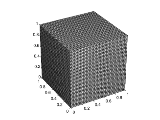
Figure 1: A uniform triangular/tetrahedron mesh on the unit square/cube.

First, we consider the system (4.1)-(4.3) on the unit square domain $\Omega=[0,1]\times[0,1]$, where $D(\mathbf{u})=\frac{1}{40}(1+|\mathbf{u}|^{2})$ and $\mu(c)=1/(1+c^{2})$. We set the terminal time $T=1.0$. The functions $f$ and $g$ are chosen correspondingly to the exact solution

$$c=1+20e^{t}(1+t^{2})\sin(x^{2})\sin(y^{2})(1-x)^{2}(1-y)^{2},$$ (4.4)

$$p=3+400e^{t}(1+t^{3})x^{2}y^{2}(1-x)^{3}(1-y)^{3}.$$ (4.5)

Numerical simulations of mixed FEM and characteristics mixed FEM with the FE space $(V^{1}_{h},S_{h}^{1},H_{h}^{1})$ were presented in [34] and [51], respectively.

Here, we solve the system (4.1)-(4.3) by the numerical scheme (2.4)-(2.6) with the lowest-order characteristics mixed FEM, in which a uniform triangular partition with $M+1$ nodes in each direction is used, see Figure 1 for an illustration with $M=8$, where $h=\sqrt{2}/M$. To show the optimal convergence rates, we choose $\tau=h^{2}$ in our numerical simulations. We present in Table 1 numerical results at $t=1.0$. From Table 1, we can observe clearly the second-order convergence rate for the concentration in $L^{2}$-norm, which is the most important physical component in applications. The convergence rate for both the pressure and Darcy velocity is $O(h)$ in $L^{2}$-norm, which is optimal in the traditional sense. The one-order lower approximation to $(p,u)$ does not affect the accuracy of the numerical concentration.

On the other hand, we resolve the system (2.11)-(2.12) with the obtained concentration $c_{h}^{N}$ for $(\widehat{p}_{h}^{N},\widehat{\bf u}_{h}^{N})\in(S_{h}^{1},H_{h}^{1})$. We present these numerical results in Table 2 from which we can see the second-order accuracy for both pressure and Darcy velocity. For comparison, we present in Table 3 numerical results of the scheme (2.4)-(2.6) with $(c_{h}^{n},p_{h}^{n},{\bf u}_{h}^{n})\in(V^{1}_{h},S_{h}^{1},H_{h}^{1})$. Numerical results show that the post-processing defined in (2.11)-(2.12) provides the same accuracy as the classical FEM solution in $(c_{h}^{n},p_{h}^{n},{\bf u}_{h}^{n})\in(V_{h}^{1},S_{h}^{1},H_{h}^{1}),n=1,2,...,N$, while the former requires much less computational cost.

To test the stability of the scheme, we solve the system (2.11)-(2.12) with several different $M$ for each $\tau=1/20,1/30,1/40$. Numerical results presented in Figure 2 illustrates that $L^{2}$-norm errors converge to $O(\tau)$ as $M$ increases. This shows that the time step restrictions given in those previous works are not necessary.

Table 1: $L^{2}$ errors of the scheme (2.4)-(2.6) with $(c_{h}^{n},p_{h}^{n},{\bf u}_{h}^{n})\in(V^{1}_{h},S_{h}^{0},H_{h}^{0})$ in 2D.

$\tau=1/M^{2}$	$\|c(\cdot,t_{N})-c_{h}^{N}\|_{L^{2}}$	$\|\mathbf{u}(\cdot,t_{N})-{\bf u}_{h}^{N}\|_{L^{2}}$	$\|p(\cdot,t_{N})-p_{h}^{N}\|_{L^{2}}$
$M=8$	3.923e-2	5.945e-1	1.532e-1
$M=16$	7.518e-3	3.020e-1	7.763e-2
$M=32$	1.704e-3	1.517e-1	3.759e-2
$M=64$	4.250e-4	7.681e-2	1.882e-1
Convergence order	2.00	0.98	1.00

Table 2: $L^{2}$-norm errors of the post-processing with $(p_{h}^{N},{\bf u}_{h}^{N})\in(S_{h}^{1},H_{h}^{1})$ in 2D.

$\tau=1/M^{2}$	$\|\mathbf{u}(\cdot,t_{N})-\widehat{\bf u}_{h}^{N}\|_{L^{2}}$	$\|p(\cdot,t_{N})-\widehat{p}_{h}^{N}\|_{L^{2}}$
$M=8$	3.299e-2	8.639e-2
$M=16$	7.025e-2	2.255e-2
$M=32$	1.588e-3	5.607e-3
$M=64$	3.871e-4	1.401e-3
order	2.04	2.00

Table 3: $L^{2}$-norm errors of scheme (2.4)-(2.6) with $(c_{h}^{n},p_{h}^{n},{\bf u}_{h}^{n})\in(V_{h}^{1},S_{h}^{1},H_{h}^{1})$ in 2D.

$\tau=1/M^{2}$	$\|\mathbf{u}(\cdot,t_{N})-\widehat{\bf u}_{h}^{N}\|_{L^{2}}$	$\|p(\cdot,t_{N})-\widehat{p}_{h}^{N}\|_{L^{2}}$
$M=8$	3.791e-2	8.625e-2
$M=16$	7.901e-3	2.221e-2
$M=32$	1.801e-3	5.601e-3
$M=64$	4.451e-4	1.423e-3
order	2.01	1.98

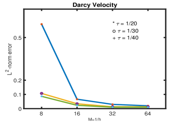
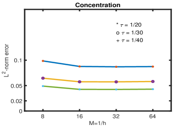
Figure 2: Stability of the scheme (2.4)-(2.6)

Secondly, we study the system (4.1)-(4.3) in a three-dimensional cube $[0,1]\times[0,1]\times[0,1]$, where $D({\bf u})=1+{\bf u}\otimes{\bf u}$ and $\mu(c)=1+c^{2}$ and the functions $f$ and $g$ are chosen correspondingly to the smooth exact solution

$$c=\frac{1}{10}\exp(-t)\sin^{2}(\pi x)\sin(\pi y)\sin(\pi z)\,,$$ (4.6)

$$p=\exp(-t)\cos(\pi x)\cos(\pi y)\cos(\pi z)\,.$$ (4.7)

We also set the terminal time T = 1.0 in this example.

We use a uniform tetrahedra mesh with $M+1$ nodes in each direction ($h=\frac{\sqrt{2}}{M}$), see Figure 1. We solve the system (4.1)-(4.3) on the unit cube with $\tau=1/512$ and $M=8,16,32$. We present our numerical results in Table 4. Numerical results confirm the second-order accuracy of concentration by the lowest characteristic-mixed FEM.

Again, after getting $c_{h}^{N}$, we resolve (4.2)-(4.3) at the terminal time $T=1.0$ with $(\widehat{{\bf u}}_{h}^{N},\widehat{p}_{h}^{N})\in(S_{h}^{1},H_{h}^{1})$. We present the $L^{2}$-norm errors of the recovered numerical solution $(\widehat{{\bf u}}_{h}^{N},\widehat{p}_{h}^{N})$ in Table 5. The second-order accuracy of numerical solution $(\widehat{{\bf u}}_{h}^{N},\widehat{p}_{h}^{N})$ is observed clearly, which confirms that the approximation for $({\bf u},p)$ in three dimensions can also be significantly improved by the proposed post-processing.

5 Conclusion

We have established optimal error estimates of the commonly-used lowest-order characteristics-mixed FEMs with linearized Euler scheme for miscible displacement problems under a weak time step condition $\tau=o(1/|\log h|)$. Previous analysis only provided a sub-optimal estimate for the concentration. We have shown theoretically and numerically that the lower-order approximation to the velocity/pressure does not pollute the numerical concentration and also, the scheme allows one to use a large time step. The analysis presented in this paper can be easily extended to other existing methods, such as ELLAM and high-order characteristic approximations. The analysis presented in this paper is based on the assumption of certain strong regularity of the solution. The problem with weaker regularity assumption is of interest. Some existing works can be found in literature, such as [1, 13] for mixed finite volume methods and [11, 19] for a framework of gradient discretization methods, including mixed FE-ELLAM and hybrid mimetic mixed-ELLAM schemes. On the other hand, theoretical analysis in this paper is based on the $\Omega$-periodic model as usual [12, 20, 23, 44, 51] to avoid the technical difficulties on the boundary. This periodic assumption is physically reasonable. For the problem with Neumann boundary conditions, some further approximation to $c_{h}^{n}(x)$ was mentioned in [44].

Table 4: $L^{2}$-norm errors of the scheme (2.4)-(2.6) with $(c_{h}^{n},p_{h}^{n},{\bf u}_{h}^{n})\in(V_{h}^{1},S_{h}^{0},H_{h}^{0})$ in 3D.

$\tau=1/512$	$c_{h}^{N}-c^{N}\|_{L^{2}}$	$\|{\bf u}_{h}^{N}-{\bf u}^{N}\|_{L^{2}}$	$\|p_{h}^{N}-p^{N}\|_{L^{2}}$
M = 8	2.441e-03	2.512e-01	4.872e-02
M = 16	6.544e-03	1.263e-01	2.451e-02
M = 32	4.422e-04	6.284e-02	1.221e-02
Order	1.94	1.00	1.00

Table 5: $L^{2}$-norm errors of the post-processing with $(\widehat{p}_{h}^{N},\widehat{\bf u}_{h}^{N})\in(S_{h}^{1},H_{h}^{1})$ in 3D .

$\tau=\frac{1}{2M}$	$\|\widehat{\bf u}_{h}^{N}-{\bf u}^{N}\|_{L^{2}}$	$\|\widehat{p}_{h}^{N}-p^{N}\|_{L^{2}}$
M = 8	1.591e-02	1.221e-02
M = 16	4.143e-03	1.012e-02
M = 32	1.046e-03	1.534e-03
Order	1.99	1.99

Acknowledgments The author would like to thank the anonymous referee for the careful review and valuable suggestions and comments, which have greatly improved this article.

References

• [1] T. Arbogast and C.S. Huang, A fully mass and volume conserving implementation of a characteristic method for transport problems, SIAM J. Sci. Comput., 28(2006), 2001–2022.
• [2] M. Al-Lawatia, R.C. Sharpley and H. Wang, Second-order characteristic methods for advection-diffusion equations and comparison to other schemes, Adv. Water. Resour., 22 (1999), 741-768.
• [3] J. Bear and Y. Bachmat, Introduction to Modeling of Transport Phenomena in Porous Media, Springer-Verlag, New York, 1990.
• [4] A. Bermudez, M.R. Nogueiras and C. Vazquez, Numerical analysis of convection-diffusion-reaction problems with higher order characteristics/finite elements. II. Fully discretized scheme and quadrature formulas, SIAM J. Numer. Anal., 44 (2006), 1854-1876.
• [5] S. Brenner and L. Scott, The Mathematical Theory of Finite Element Methods, Springer, New York, 2002.
• [6] F. Brezzi, On the existence, uniquness and appproximation of saddle-point problems, arising from Lagrangian multipliers, RAIRO Anal. Numer., 2 (1974), 129–151.
• [7] W. Cai, B  Li, Y. Lin and W. Sun, Analysis of fully discrete FEMs for miscible displacement in porous media with Bear-Scheidegger diffusion-disperson tensor. Numer Math, 141 (2019), 1009–1042.
• [8] M.A. Celia, T.F. Russell, I. Herrera and R.E. Ewing, An Eulerian-Lagrangian localized adjoint method for the advection-diffusion equation, Adv. Water. Resour., 13 (1990), 187–206.
• [9] F. Chen, H. Chen and H. Wang, An optimal-order error estimate for a Galerkin-mixed finite element time-stepping procedure for porous media flows, Numer. Methods Partial Differ. Equations, 28.2(2012), 707–719.
• [10] A. Cheng, K. Wang and H. Wang, Superconvergence for a time-discretization procedure for the mixed finite element approximation of miscible displacement in porous media, Numer. Methods Partial Differ. Equations, 28(2012), 1382–1398.
• [11] H. M. Cheng, J. Droniou and K.N. Le, Convergence analysis of a family of ELLAM schemes for a fully coupled model of miscible displacement in porous media, Numer. Math., 141(2019), 353–397.
• [12] C.N. Dawson, T.F. Russell and M.F. Wheeler, Some improved error estimates for the modified method of characteristics, SIAM J. Numer. Anal., 26 (1989), 1487-1512.
• [13] M.  D’Elia, M. Perego, P. Bochev and D. Littlewood, A coupling strategy for nonlocal and local diffusion models with mixed volume constraints and boundary conditions, Comput. Math. Appl., 71 (2016), 2218–2230.
• [14] L. Demkowicz and J.T. Oden, An adaptive characteristic Petrov-Galerkin finite element method for convection-dominated linear and nonlinear parabolic problems in one space variable, J. Comput. Phys., 67 (1986), 188-213.
• [15] J. Douglas, Jr., R.E. Ewing and M.F. Wheeler, The approximation of the pressure by a mixed method in the simulation of miscible displacement RAIRO Anal. Numer., 17 (1983), 17–33.
• [16] J. Douglas, Jr., R.E. Ewing and M.F. Wheeler, A time-discretization procedure for a mixed finite element approximation of miscible displacement in porous media, RAIRO Anal. Numer., 17 (1983), 249-265.
• [17] J. Douglas, Jr. and T.F. Russell, Numerical methods for convection-dominated diffusion problems based on combining the method of characteristics with finite element or finite difference procedures, SIAM J. Numer. Anal., 19 (1982), 871-885.
• [18] J. Douglas, JR., and J. E. Roberts, Global estimates for mixed methods for second order elliptic equations, Math. Comput., 44(1985), 39–52.
• [19] J.  Droniou, R. Eymard, A. Prignet and K. S. Talbot, Unified convergence analysis of numerical schemes for a miscible displacement problem, Found. Comput. Math., 19(2019), 333–374.
• [20] R.G. Duran, On the approximation of miscible displacement in porous media by a method of characteristics combined with a mixed method, SIAM J. Numer. Anal., 25 (1988), 989-1001.
• [21] R.G. Duran, Error analysis in $L^{p}$, $1\leq p\leq\infty$, for mixed finite element methods for linear and quasi-linear elliptic problems, RAIRO Mod. Math. Anal. Numer. , 22(1988), 371–387.
• [22] R. E. Ewing, ed, The mathematics of Reservoir Simulation, Frontiers in Applied Mathematics, SIAM, Philadelphia, PA, 1983.
• [23] R.E. Ewing, T.F. Russell and M.F. Wheeler, Convergence analysis of an approximation of miscible displacement in porous media by mixed finite elements and a modified method of characteristics, Comput. Methods Appl. Mech. Engrg., 47 (1984), 73-92.
• [24] R. E. Ewing and H. Wang, A summary of numerical methods for time-dependent advection-dominated partial differential equations, J. Comput. Appl. Math., 128 (2001), 423-445.
• [25] R.E. Ewing and M.F. Wheeler, Galerkin methods for miscible displacement problems in porous media, SIAM J. Numer. Anal., 17 (1980), 351-365.
• [26] X. Feng, On existence and uniqueness results for a coupled system modeling miscible displacement in porous media, J. Math. Anal. Appl., 194 (1995), 883–910.
• [27] X. Feng and M. Neilan, A modified characteristic finite element method for a fully nonlinear formulation of the semigeostrophic flow equations, SIAM J. Numer. Anal., 47 (2009), 2952-2981.
• [28] A.O. Garder, D.W. Peaceman and A.L. Pozzi, Numerical calculations of multidimensional miscible displacement by the method of characteristics, Soc. Pet. Eng. J., 4 (1964), 26-36.
• [29] H. Gao and W. Sun, Optimal error analysis of Crank-Nicolson lowest-order Galerkin-mixed FEM for incompressible miscible flow in porous media, Numerical Methods for PDEs, 36(2020), 1773–1789.
• [30] L. Gastaldi and R. H. Nochetto, Sharp maximum norm error estimates for general mixed finite element approximations to second order elliptic equations, M2AN, 23 (1989), 103–128.
• [31] J. Kacur and M.S. Mahmood, Solution of solute transport in unsaturated porous media by the method of characteristics, Numer. Methods Partial Differential Equations, 19(2003), 732-761.
• [32] S. V. Krishnamachari, L. J. Hayes and T. F. Russell, A finite element alternating-direction method combined with a modified method of characteristics for convection-diffusion problems, SIAM J. Numer. Anal., 26 (1989), 1462-1473.
• [33] S. Kumar and S. Yadav, Modified method of characteristics combined with finite volume element methods for incompressible miscible displacement problems in porous media, Int. J. Partial. Differ. Equ., 2014.
• [34] B. Li and W. Sun, Error analysis of linearized semi-implicit Galerkin finite element methods for nonlinear parabolic equations, Int. J. Numer. Anal. Model., 10 (2013), 622-633.
• [35] B. Li and W. Sun, Unconditional convergence and optimal error estimates of a Galerkin-mixed FEM for incompressible miscible flow in porous media, SIAM J. Numer. Anal., 51 (2013), 1959-1977.
• [36] B. Li and W. Sun, Regularity of the diffusion-dispersion tensor and error analysis of FEMs for a porous media flow, SIAM J. Numer. Anal., 53(2015), 1418–1437.
• [37] B. Li, J. Wang and W. Sun, The stability and convergence of fully discrete Galerkin FEMs for incompressible miscible flows in porous media, Commun. Comput. Phys., 15(2014), 1141–1158.
• [38] D. Liang, W. Wang and Y. Cheng, An efficient second-order characteristic finite element method for non-linear aerosol dynamic equations, Int. J. Numer. Methods Engrg., 80 (2009), 338-354.
• [39] N. Ma, T. Lu and D. Yang, Analysis of incompressible miscible displacement in porous media by characteristics collocation method, Numer. Methods Partial Differential Equations, 22 (2006), 797-814.
• [40] A.  Mohamed and A.K. Pani, An H1-Galerkin mixed finite element method combined with the modified method of characteristics for incompressible miscible displacement problems in porous media. New directions in applied mathematics (Hyderabad, 1995), Differential Equations Dynam. Systems, 6(1998), 135-147.
• [41] L. Nirenberg, An extended interpolation inequality, Ann. Scuola Norm. Sup. Pisa(3), 20 (1966), 733-737
• [42] D.W. Peaceman, Fundamentals of Numerical Reservior Simulations, Elsevier, Amsterdam, 1977.
• [43] P.A. Raviart and J.M. Thomas, A mixed finite element method for 2nd order elliptic problems, Mathematical Aspects of Finite Element Methods, Lecture Notes in Math. 606, Springer-Verlag, Berlin, (1977), 292-315.
• [44] T. F. Russell, Time stepping along characteristics with incomplete iteration for a Galerkin approximation of miscible displacement in porous media, SIAM J. Numer. Anal., 22 (1985), 970-1013.
• [45] G. Scovazzi, M.F. Wheeler, A. Mikelic and S. Lee, Analytical and variational numerical methods for unstable miscible displacement flows in porous media, J. Comput. Phys., 335(2017), 444–496.
• [46] Z. Si, J. Wang and W. Sun. Unconditional stability and error estimates of modified characteristics FEMs for the Navier-Stokes equations, Numer. Math., 134(2016), 139–161.
• [47] T. Sun and Y. Yuan, An approximation of incompressible miscible displacement in porous media by mixed finite element method and characteristics-mixed finite element method, J. Comput. Appl. Math., 228 (2009), 391-411.
• [48] W. Sun and C. Wu, New analysis and optimal error estimates of Galerkin-mixed FEMs for incompressible miscible flow in porous media, Math. Comput., 2021 DOI: https://doi.org/10.1090/mcom/3561.
• [49] H. Wang, An optimal-order error estimate for a family of ELLAM-MFEM approximations to porous medium flow, SIAM J. Numer. Anal., 46 (2008), 2133–2152.
• [50] H. Wang, R.E. Ewing and T.F. Russell, Eulerian-Lagrangian localized adjoint methods for convection-diffusion equations and their convergence analysis, IMA J. Numer. Anal., 15 (1995), 405–459.
• [51] J. Wang, Z. Si and W. Sun, A new error analysis of characteristics-mixed FEMs for miscible displacement in porous media, SIAM J. Numer. Anal., 52(2014), 3300–3020.
• [52] M.F. Wheeler, A priori $L^{2}$ error estimates for Galerkin approximations to parabolic partial differential equations, SIAM J. Numer. Anal., 10 (1973), 723–759.