Discrete energy analysis of the third-order variable-step BDF time-stepping for diffusion equations

Abstract

This is one of our series works on discrete energy analysis of the variable-step BDF schemes. In this part, we present stability and convergence analysis of the third-order BDF (BDF3) schemes with variable steps for linear diffusion equations, see e.g. [SIAM J. Numer. Anal., 58:2294-2314] and [Math. Comp., 90: 1207-1226] for our previous works on the BDF2 scheme. To this aim, we first build up a discrete gradient structure of the variable-step BDF3 formula under the condition that the adjacent step ratios are less than 1.4877, by which we can establish a discrete energy dissipation law. Mesh-robust stability and convergence analysis in the $L^{2}$ norm are then obtained. Here the mesh robustness means that the solution errors are well controlled by the maximum time-step size but independent of the adjacent time-step ratios. We also present numerical tests to support our theoretical results.
Keywords: diffusion equations, variable-step third-order BDF scheme, discrete gradient structure, discrete orthogonal convolution kernels, stability and convergence
AMS subject classifications: 65M06, 65M12

1 Introduction

In this paper, we aim to develop a discrete energy technique for the stability and convergence of three-step backward differentiation formula (BDF3) with variable time-steps. To this end, we consider the linear reaction-diffusion problem in a bounded convex domain $\Omega$,

$$\partial_{t}u-\varepsilon\Delta u =\kappa(x)u+f(t,x)\quad\text{for $x\in\Omega$ and $0<t<T$,}$$ (1.1)

subject to the Dirichlet boundary condition $u=0$ on a smooth boundary $\partial\Omega$, and the initial data $u(0,x)=u_{0}$ for $x\in\Omega$. We assume that the diffusive coefficient $\varepsilon>0$ is a constant and the reaction coefficient $\kappa(x)$ is smooth and bounded by $\kappa^{*}>0$.

The BDF schemes are widely used for stiff or differential-algebraic problems [7, 8]. Recently, they were also applied for simulating hyperbolic systems with multiscale relaxation [1] and stiff kinetic equations [5]. For such applications, BDF schemes with variable steps are shown to be computationally efficient in capturing the multi-scale time behaviors [2, 4, 6, 8, 10, 1, 16]. However, rigorous theoretically analysis (stability and convergence) for variable-step BDF schemes is challenging. This motivates our serious works on this topic, and one can find our previous works on the variable-step BDF2 scheme [13, 11].

To begin, we consider the temporal mesh

$$0=t_{0}<t_{1}<t_{2}<\cdots<t_{N}=T$$

with the variable time-step

$$\tau_{k}:=t_{k}-t_{k-1},\quad 1\leq k\leq N.$$

The maximum step size and the adjacent time-step ratios are defined respectively as

$$\tau:=\max_{1\leq k\leq N}\tau_{k},\quad r_{k}:=\frac{\tau_{k}}{\tau_{k-1}}\,\,\,\textmd{for}\,\,\,2\leq k\leq N.$$

For any sequences $\{v^{n}\}_{n=0}^{N}$, we denote $\partial_{\tau}v^{n}:=(v^{n}-v^{n-1})/\tau_{n}$. Then by taking $v^{n}=v(t_{n})$, the variable-step BDF3 formula [3] yields

$$D_{3}v^{n}= \,d_{0}(r_{n},r_{n-1})\partial_{\tau}v^{n}+d_{1}(r_{n},r_{n-1})\partial_{\tau}v^{n-1}+d_{2}(r_{n},r_{n-1})\partial_{\tau}v^{n-2},$$ (1.2)

where

$$d_{0}(x,y):= \,\frac{1+2x}{1+x}+\frac{xy}{1+y+xy},$$ (1.3)

$$d_{1}(x,y):= \,-\frac{x}{1+x}-\frac{xy}{1+y+xy}-\frac{xy^{2}}{1+y+xy}\frac{1+x}{1+y},$$ (1.4)

$$d_{2}(x,y):= \,\frac{xy^{2}}{1+y+xy}\frac{1+x}{1+y},\qquad\text{for $x,y\geq 0$.}$$ (1.5)

Without losing the generality, we assume that the discrete solution $u^{1}$ and $u^{2}$ are given. We now consider a time-discrete solution for the diffusion equations, $u^{k}(x)\approx u(t_{k},x)$ for $x\in\Omega$, by the following variable-step BDF3 time-stepping scheme

$$D_{3}u^{k}=\varepsilon\Delta u^{k}+\kappa u^{k}+f^{k},\quad,3\leq k\leq N,$$ (1.6)

where $f^{k}(x)=f(t_{k},x)$.

To the best of our knowledge, there are very few theoretical results on the variable-step BDF3 scheme in literature. For linear diffusion problems, Calvo and Grigorieff [3] established the following $L^{2}$ norm stability estimate under the step-ratio condition $r_{k}<1.199$,

$$\big{\|}u^{n}\big{\|}\leq C\exp\left(C\Gamma_{n}\right)\Big{(}\big{\|}u_{0}\big{\|}+\sum_{j=1}^{n}\tau_{j}\big{\|}f^{j}\big{\|}\Big{)}\quad\text{for $n\geq 1$,}$$

where the ratio-dependent prefactor $\Gamma_{n}$ is given by

$$\Gamma_{n}:=\sum_{k=2}^{n}\big{|}r_{k}-r_{k-1}\big{|}.$$

This means that any mixture of the $k$-step BDF $(k\in\{1,2,3\})$ is stable provided the number of changes between increasing and decreasing mesh-sizes is uniformly bounded. Nonetheless, the quantity $\exp\left(C\Gamma_{n}\right)$ can be unbounded since $\Gamma_{n}$ could blow up for certain time-step series at vanishing time-steps. To see this, we consider a specific class of time-steps $\{\cdots,\tau_{1},\mu\tau_{1},\tau_{1},\mu\tau_{1},\cdots\}$ with a positive constant $\mu\neq 1$. Then for a finite time $T=\frac{M}{2}(1+\mu)\tau_{1}$, one has

$$\Gamma_{M}=\sum_{k=2}^{M}\big{|}\mu-\mu^{-1}\big{|}=(M-1)\big{|}\mu-\mu^{-1}\big{|}\rightarrow\infty\qquad\text{as $\tau_{1}\rightarrow 0$}.$$

To remedy this issue, we present shall in this work a new framework for analyzing the variable step BDF3 scheme. Our contribution is two folds:

• We build up a discrete graident structure of BDF3 formula under the step-ratio condition $0<r_{k}<R_{e}$, where $R_{e}\approx 1.4877$ is the unique positive root of

  $$d_{1}(R_{e},0)+\tfrac{7}{10}\sqrt{R_{e}}d_{2}(R_{e},R_{e})=0.$$

  Based on this, we present the discrete energy stability for the variable-step BDF3 scheme.

• We further present the stability and convergence analysis in the $L^{2}$ norm for the BDF3 scheme under the adjacent step ratios $0<r_{k}<R_{e}.$ We also show that these analysis results are mesh-robustly, which means that the associated prefactors in our analysis are independent of the time-step ratios $r_{k}$. That is, unbounded quantities such as $\Gamma_{n}$ in [3] are removed.

The rest of this work is organized as following. In the next section, we provide with some preliminary tools, e.g., discrete orthogonal convolution kernels, for our analysis. In section 3, we present the energy stability of the variable-step BDF3 scheme. The stability and convergence analysis of the variable-step BDF3 scheme is then presented in section 4. This is followed by some numerical examples in section 5.

2 Discrete orthogonal convolution kernels

In this section, we present some preliminary tools for our analysis. We remark that the mesh-robust stability and convergence of the variable-step BDF2 scheme have been established in our previous works [10, 13]. Nonetheless, the extension to BDF3 formula is theoretically challenging due to the additional degrees of freedom. This work is builds upon our previous work [9], where the stability of variable-step BDF3 method for nonlinear ODE problems was verified under the step-ratio condition $r_{k}<R_{3}\approx 2.553$.

To begin, we write the BDF3 formula (1.2) as a convolution of local difference quotients

$$D_{3}v^{n}:=\sum_{j=1}^{n}d^{(n)}_{n-j}\partial_{\tau}v^{j}\quad\text{for $n\geq 3$,}$$ (2.7)

where the associated discrete BDF3 kernels

$$d^{(n)}_{j}:=d_{j}(r_{n},r_{n-1})\;\;\text{for $j=0,1,2$,}\quad\text{and}\quad d^{(n)}_{j}:=0\quad\text{for $n\geq j+1\geq 4$}.$$ (2.8)

Assume always that the summation $\sum_{k=i}^{j}\cdot$ to be zero and the product $\prod_{k=i}^{j}\cdot$ to be one if the index $i>j$. As for the BDF3 kernels $d^{(n)}_{n-j}$ with any fixed indexes $n$, we recall a class of discrete orthogonal convolution (DOC) kernels $\big{\{}\vartheta_{n-j}^{(n)}\big{\}}_{j=3}^{n}$ by a recursive procedure, also see [13],

$$\vartheta_{0}^{(n)}:=\frac{1}{d^{(n)}_{0}}\quad\text{and}\quad\vartheta_{n-j}^{(n)}:=-\frac{1}{d^{(j)}_{0}}\sum_{i=j+1}^{n}\vartheta_{n-i}^{(n)}d^{(i)}_{i-j}\quad\text{for $3\leq j\leq n-1$.}$$ (2.9)

Obviously, the DOC kernels $\vartheta_{n-j}^{(n)}$ satisfy the following discrete orthogonality identity

$$\sum_{i=j}^{n}\vartheta_{n-i}^{(n)}d^{(i)}_{i-j}\equiv\delta_{nj}\quad\text{for any $3\leq j\leq n$,}$$ (2.10)

where $\delta_{nj}$ is the Kronecker delta symbol with $\delta_{nj}=0$ if $j\neq n$. Furthermore, with the identity matrix $I_{m\times m}$ ($m:=n-2$), the above discrete orthogonality identity (2.10) also implies

$$\Theta_{3}D_{3}=I_{m\times m},$$

where the two $m\times m$ matrices $D_{3}$ and $\Theta_{3}$ are defined by

$$D_{3}:=\left(\begin{array}[]{cccc}d_{0}^{(3)}&&&\\ d_{1}^{(4)}&d_{0}^{(4)}&&\\ \vdots&\vdots&\ddots&\\ d_{n-3}^{(n)}&d_{n-2}^{(n)}&\cdots&d_{0}^{(n)}\\ \end{array}\right)\;\;\text{and}\;\;\Theta_{3}:=\left(\begin{array}[]{cccc}\vartheta_{0}^{(3)}&&&\\ \vartheta_{1}^{(4)}&\vartheta_{0}^{(4)}&&\\ \vdots&\vdots&\ddots&\\ \vartheta_{n-3}^{(n)}&\vartheta_{n-2}^{(n)}&\cdots&\vartheta_{0}^{(n)}\\ \end{array}\right).$$

Obviously, one has $D_{3}\Theta_{3}=I_{m\times m},$ which implies the following mutual orthogonality identity

$$\sum_{i=j}^{n}d_{n-i}^{(n)}\vartheta^{(i)}_{i-j}\equiv\delta_{nj}\quad\text{for any $3\leq j\leq n$.}$$ (2.11)

Note that, this identity (2.11) will be used to study the discrete property of DOC kernels; while the above identity (2.10) will be used to reformulate the discrete scheme (1.6). By exchanging the summation order and using (2.10), one has

$$\sum_{i=3}^{n}\vartheta_{n-i}^{(n)}D_{3}v^{i}= \,\sum_{i=3}^{n}\vartheta_{n-i}^{(n)}\sum_{j=1}^{2}d^{(i)}_{i-j}\partial_{\tau}v^{j}+\sum_{i=3}^{n}\vartheta_{n-i}^{(n)}\sum_{j=3}^{i}d^{(i)}_{i-j}\partial_{\tau}v^{j}$$

$$= \,\sum_{j=1}^{2}\partial_{\tau}v^{j}\sum_{i=3}^{n}\vartheta_{n-i}^{(n)}d^{(i)}_{i-j}+\sum_{j=3}^{n}\partial_{\tau}v^{j}\sum_{i=j}^{n}\vartheta_{n-i}^{(n)}d^{(i)}_{i-j}$$

$$= \,\mathcal{I}_{3}^{n}[v]+\partial_{\tau}v^{n}\qquad\text{for $n\geq 3$,}$$ (2.12)

where $\mathcal{I}_{3}^{n}[v]$ represents the starting effect on the numerical solution at $t_{n}$, or

$$\mathcal{I}_{3}^{n}[v]:= \,\sum_{j=1}^{2}\partial_{\tau}v^{j}\sum_{i=3}^{n}\vartheta_{n-i}^{(n)}d^{(i)}_{i-j}=\partial_{\tau}v^{2}\sum_{i=3}^{n}\vartheta_{n-i}^{(n)}d^{(i)}_{i-2}+\vartheta_{n-3}^{(n)}d^{(3)}_{2}\partial_{\tau}v^{1}\quad\text{for $n\geq 3$.}$$ (2.13)

Multiplying both sides of the equation (1.6) by the DOC kernels $\vartheta_{n-k}^{(n)}$, and summing $k$ from $3$ to $n$, we apply (2) to get the following equivalent form

$$\partial_{\tau}u^{n}=-\mathcal{I}_{3}^{n}[u]+\sum_{k=3}^{n}\vartheta_{n-k}^{(n)}\left(\varepsilon\Delta u^{k}+\kappa u^{k}\right)+\sum_{k=3}^{n}\vartheta_{n-k}^{(n)}f^{k}\quad\text{for $3\leq n\leq N$.}$$ (2.14)

This formulation expresses the BDF3 solution at time $t_{n}$ as a (global) convolution summation of all previous solutions with DOC kernels $\vartheta_{n-k}^{(n)}$ as the convolutional weights.

Next section constructs a discrete gradient structure of variable-step BDF3 formula and derives the energy stability of BDF3 scheme via the original form (1.6). Section 3 addresses the $L^{2}$ norm stability and convergence analysis via the discrete convolution form (2.14). Some numerical examples are presented in the last section to support our theoretical results.

3 Positive definiteness and energy stability

To show the energy stability of the variable-step BDF3 scheme, we first investigate sufficient conditions on the adjacent time-step ratios $r_{k}$ so that the discrete kernels $\big{\{}\tau_{n}d_{n-k}^{(n)}\big{\}}$ are positive definite.

For certain adaptive time-stepping process, one may choose the step size $\tau_{m+1}$ (or the step ratio $r_{m+1}$) properly according to the information from previous time-step ratios $\{r_{k}\}_{k=2}^{m}$. Actually, the positive definiteness should be determined by the eigenvalues of the pentadiagonal symmetric matrix $B_{3}=B_{L}+B_{L}^{T}$, where

$$B_{L}:=\left(\begin{array}[]{ccccc}\tau_{3}d_{0}^{(3)}&&&&\vspace{0.15cm}\hfil\\ \tau_{4}d_{1}^{(4)}&\tau_{4}d_{0}^{(4)}&&&\vspace{0.15cm}\hfil\\ \tau_{5}d_{2}^{(5)}&\tau_{5}d_{1}^{(5)}&\tau_{5}d_{0}^{(5)}&&\vspace{0.15cm}\hfil\\ &\ddots&\ddots&\ddots&\vspace{0.1cm}\hfil\\ &&\tau_{n}d_{2}^{(n)}&\tau_{n}d_{1}^{(n)}&\tau_{n}d_{0}^{(n)}\\ \end{array}\right).$$ (3.6)

A sufficient and necessary condition for the positive definiteness of $B_{3}$ would be a certain combination involving all time-step ratios; however, it remains open at this moment. We consider only certain restriction of each step ratio, like $0<r_{k}<R_{e}$ for a fixed positive constant $R_{e}<R_{3}\approx 2.553$, the recent stability constraint [9] for the ODE problems.

Table 1: Minimum eigenvalue of step-rescaled matrix $\widetilde{B}_{3}$ on random meshes.

  $n$ $R_{e}=1.20$ $R_{e}=1.50$ $R_{e}=1.69$ $R_{e}=1.70$ 50 1.12 5.08e-01 6.12e-02 -4.55e-02 100 1.07 4.35e-01 4.58e-02 -5.29e-02 200 1.08 4.18e-01 -2.06e-02 -8.49e-02  

Numerical tests on random meshes are performed to examine the positive definiteness of $B_{3}$ via the step-rescaled matrix $\widetilde{B}_{3}:=\Lambda_{\tau}^{-1}(B_{L}+B_{L}^{T})\Lambda_{\tau}^{-1}$, where $\Lambda_{\tau}=\mathrm{diag}(\sqrt{\tau_{3}},\sqrt{\tau_{4}},\cdots,\sqrt{\tau_{n}})$. We take a finite time $T=1$ with $n$ grid points and let $r_{k}$ $(2\leq k\leq n)$ be uniformly distributed random numbers over $(0,R_{e})$. Table 1 lists the minimum eigenvalue (each data is the minimum value of 200 runs on different random meshes) of $\widetilde{B}_{3}$ for the fixed step-ratio limits $R_{e}=1.20$, $1.50$, $1.69$ and $1.70$. To ensure the positive definiteness, Table 1 suggests that the maximum step-ratio limit $R_{e}<1.69$ is necessary, while we will prove theoretically that $R_{e}<1.4877$ is sufficient in the next subsection.

3.1 Discrete gradient structure

To derive the energy stability of numerical scheme, we need a discrete gradient structure of variable-step BDF3 formula. In the following, we will seek two nonnegative quadratic functionals $G$ and $F$ such that

$$J_{n}:=2v_{n}\tau_{n}\sum_{j=3}^{n}d_{n-j}^{(n)}v_{j}=G[v_{n},v_{n-1}]-G[v_{n-1},v_{n-2}]+F[v_{n},v_{n-1},v_{n-2}],$$ (3.7)

for $n\geq 3$, where the discrete BDF3 kernels $d_{j}^{(n)}$ are defined by (2.8), such that the associated quadratic form is positive definite

$$2\sum_{k=3}^{n}v_{k}\tau_{k}\sum_{j=3}^{k}d_{k-j}^{(k)}v_{j}>0\quad\text{if $v_{k}\not\equiv 0$.}$$

This seems to be a difficult task due to the presence of variable kernels $d_{j}^{(n)}$, refer to the recent comments in [6, section 3.4]. For the uniform case with $r_{k}\equiv 1,$ it has been shown in [14] that the uniform BDF3 formula admits the following discrete gradient structure

$$2v_{n}\Big{(}\frac{11}{6}v_{n}-\frac{7}{6}v_{n-1}+\frac{1}{3}v_{n-2}\Big{)}= \,\frac{1}{3}v_{n}^{2}+\frac{1}{3}(\tfrac{7}{4}v_{n}-v_{n-1})^{2}-\left[\frac{1}{3}v_{n}^{2}+\frac{1}{3}(\tfrac{7}{4}v_{n}-v_{n-1})^{2}\right]$$

$$\,+\frac{95}{48}v_{n}^{2}+\frac{1}{3}(v_{n}-\tfrac{7}{4}v_{n-1}+v_{n-2})^{2}.$$

This decomposition is optimal in the sense that the minimum eigenvalue bound $\frac{95}{48}$ of the associated quadratic form is sharp, see [12, Lemma 2.4], due to the Grenander-Szegö theorem.

To deal with the variable-step case, our first task is to introduce a step-rescale transform $v_{j}=w_{j}/\sqrt{\tau_{j}}$ for $j\geq 1$, cf. the above step-rescaled matrix $\widetilde{B}_{3}$, to remove the time-step factor $\tau_{n}$ in the discrete kernels of (3.7). One can get

$$J_{n}=2w_{n}\sum_{j=3}^{n}\tilde{d}_{n-j}^{(n)}w_{j}\quad\text{with}\quad\tilde{d}_{n-j}^{(n)}:=\frac{\sqrt{\tau_{n}}}{\sqrt{\tau_{j}}}d_{n-j}^{(n)}\quad\text{for $n\geq j+2\geq 3$}.$$ (3.8)

It is reasonable to assume that

$$\widetilde{G}[w_{n},w_{n-1}]:= \,a_{n+1}w_{n}^{2}+b_{n+1}(\gamma w_{n}-w_{n-1})^{2},$$

$$\widetilde{F}[w_{n},w_{n-1},w_{n-2}]:= \,p_{n+1}w_{n}^{2}+q_{n+1}(\gamma w_{n}-w_{n-1})^{2}+c_{n}\big{(}w_{n}-\gamma w_{n-1}+w_{n-2}\big{)}^{2},$$

where the nonnegative variable coefficients $a_{n},b_{n},c_{n},p_{n},q_{n}$ and the real parameter $\gamma$ (for which $\gamma=7/4$ would not necessarily be optimal) is determined such that

$$J_{n}=\widetilde{G}[w_{n},w_{n-1}]-\widetilde{G}[w_{n-1},w_{n-2}]+\widetilde{F}[w_{n},w_{n-1},w_{n-2}].$$ (3.9)

The principle of identity gives the following relationships for the undetermined coefficients:

coefficients of $$w_{n}w_{n-2} \,2c_{n}=2\tilde{d}_{2}^{(n)};$$:

coefficients of $$w_{n-2}^{2} w_{n-1}w_{n-2} \,-b_{n}+c_{n}=0;$$ ():

coefficients of $$w_{n}w_{n-1} \,-2\gamma(b_{n+1}+q_{n+1})-2\gamma c_{n}=2\tilde{d}_{1}^{(n)};$$:

coefficients of $$w_{n-1}^{2} \,-a_{n}+(b_{n+1}+q_{n+1})-\gamma^{2}b_{n}+\gamma^{2}c_{n}=0;$$:

coefficients of $$w_{n}^{2} \,a_{n+1}+p_{n+1}+\gamma^{2}(b_{n+1}+q_{n+1})+c_{n}=2\tilde{d}_{0}^{(n)}.$$:

They yield that

$$a_{n}=-\frac{1}{\gamma}\tilde{d}_{1}^{(n)}-\tilde{d}_{2}^{(n)},\quad b_{n}=\tilde{d}_{2}^{(n)},\quad c_{n}=\tilde{d}_{2}^{(n)},$$

$$p_{n+1}=2\tilde{d}_{0}^{(n)}+\gamma\tilde{d}_{1}^{(n)}+(\gamma^{2}-1)\tilde{d}_{2}^{(n)}+\frac{1}{\gamma}\tilde{d}_{1}^{(n+1)}+\tilde{d}_{2}^{(n+1)},$$

$$q_{n+1}=a_{n}-b_{n+1}=-\frac{1}{\gamma}\tilde{d}_{1}^{(n)}-\tilde{d}_{2}^{(n)}-\tilde{d}_{2}^{(n+1)}.$$

According to the definitions in (3.8) and (2.8), the coefficients $b_{n}$ and $c_{n}$ are always positive, while $a_{n}$ is also positive if $q_{n+1}\geq 0$. Thus the above assumption (3.9) requires

$$q_{n+1}= \,-\frac{1}{\gamma}\tilde{d}_{1}^{(n)}-\tilde{d}_{2}^{(n)}-\tilde{d}_{2}^{(n+1)}\geq 0,$$ (3.10)

$$p_{n+1}= \,2\tilde{d}_{0}^{(n)}-\tilde{d}_{2}^{(n)}+\gamma^{2}\Big{(}\frac{1}{\gamma}\tilde{d}_{1}^{(n)}+\tilde{d}_{2}^{(n)}\Big{)}+\frac{1}{\gamma}\tilde{d}_{1}^{(n+1)}+\tilde{d}_{2}^{(n+1)}>0\quad\text{for all $r_{k}<R_{e}$.}$$ (3.11)

The inequality system (3.10)-(3.11) involves five independent variables $r_{n+1}$, $r_{n}$, $r_{n-1}$, $\gamma$ and the step-ratio limit $R_{e}$. In general, we are not able to solve it exactly to determine the optimal values of $\gamma$ so that the resulting step-ratio limit $R_{e}$ is as large as possible. As done in previous studies [2, 9], we consider a specific grid with constant step-ratio $r_{k}=r$ for a rough estimate of $\gamma$. In such case the first condition (3.10) becomes

$$\gamma\leq\frac{-d_{1}(r,r)}{2\sqrt{r}d_{2}(r,r)}\quad\text{for all $r<R_{e}$.}$$

An obvious choice is $\tilde{\gamma}=\frac{-d_{1}(\tilde{R}_{e},\tilde{R}_{e})}{2\sqrt{\tilde{R}_{e}}d_{2}(\tilde{R}_{e},\tilde{R}_{e})}$ ($\tilde{\gamma}$ is decreasing with repect to $\tilde{R}_{e}$), but the parameter $\tilde{\gamma}$ is not sufficient to ensure (3.10). Actually, we take $r_{n-1}=0$ and $r_{n+1}=r_{n}=\tilde{R}_{e}$ and get

$$-\frac{\sqrt{\tilde{R}_{e}}}{\tilde{\gamma}}d_{1}(\tilde{R}_{e},0)-\tilde{R}_{e}d_{2}(\tilde{R}_{e},\tilde{R}_{e})=\frac{-\tilde{R}_{e}^{4}(\tilde{R}_{e}^{3}+\tilde{R}_{e}^{2}-1)}{(\tilde{R}_{e}^{2}+\tilde{R}_{e}+1)(\tilde{R}_{e}^{3}+3\tilde{R}_{e}^{2}+2\tilde{R}_{e}+1)}<0$$

if the step-ratio limit $\tilde{R}_{e}\geq 1$, so that the desired condition (3.10) is invalid. In turn, taking $r_{n-1}=0$ and $r_{n+1}=r_{n}=r$ in (3.10) yields

$$\gamma\leq\frac{-d_{1}(r,0)}{\sqrt{r}d_{2}(r,r)}\quad\text{for all $r<R_{e}$.}$$

It introduces a reliable choice ($\bar{\gamma}$ is also decreasing with respect to $\bar{R}_{e}$)

$$\bar{\gamma}:=\frac{-d_{1}(\bar{R}_{e},0)}{\sqrt{\bar{R}_{e}}d_{2}(\bar{R}_{e},\bar{R}_{e})}.$$

Consider the second condition (3.11) with $\gamma=\bar{\gamma}$ and $r_{n+1}=r_{n}=r_{n-1}=\bar{R}_{e}$. Thus we can determine the value of $\bar{R}_{e}$ by assuming that

$$2d_{0}(\bar{R}_{e},\bar{R}_{e})-R_{e}d_{2}(\bar{R}_{e},\bar{R}_{e})+\bar{\gamma}^{2}\Big{(}\frac{1}{\bar{\gamma}}\sqrt{\bar{R}_{e}}d_{1}(\bar{R}_{e},\bar{R}_{e})+R_{e}d_{2}(\bar{R}_{e},\bar{R}_{e})\Big{)}$$

$$+\frac{1}{\bar{\gamma}}\sqrt{\bar{R}_{e}}d_{1}(\bar{R}_{e},\bar{R}_{e})+\bar{R}_{e}d_{2}(\bar{R}_{e},\bar{R}_{e})=0.$$

We solve this equation numerically and find the unique positive roots $\bar{R}_{e}\approx 1.4965$ with the corresponding parameter $\bar{\gamma}\approx 0.6924$.

To simplify the subsequent mathematical derivations, we fix the parameter $\gamma=7/10$ which is very close to $\bar{\gamma}\approx 0.6924$. The corresponding maximum step-ratio $R_{e}$ is determined by

$$d_{1}(R_{e},0)+\frac{7}{10}\sqrt{R_{e}}d_{2}(R_{e},R_{e})=0\quad\text{or}\quad\frac{10}{7\left(R_{e}+1\right)}-\frac{R_{e}^{2}\sqrt{R_{e}}}{R_{e}^{2}+R_{e}+1}=0.$$

We solve this equation numerically and find the unique positive root $R_{e}\approx 1.4877.$ This choice is mainly because the restirction (3.10) should be necessary and sharp, while the inequality (3.11) can be relaxed appropriately.

We are now ready to prove the following lemma, which gives the discrete gradient structre. Note that, the complex conditions (3.10)-(3.11) make the proof tedious and lengthy and some technical lemmas are included in Appendix A.

Lemma 3.1.

Define the following functions

$$d_{*}(x,y):= \,-\frac{10}{7}\sqrt{x}d_{1}(x,y)-\sqrt{xy}d_{2}(x,y),\quad$$ (3.12)

$$p(x,y,z):= \,2d_{0}(y,z)-\sqrt{yz}d_{2}(y,z)-\frac{49}{100}d_{*}(y,z)-d_{*}(x,y),$$ (3.13)

$$q(x,y,z):= \,d_{*}(y,z)-\sqrt{xy}d_{2}(x,y),\qquad\text{for $0<x,y,z<R_{e}$}$$ (3.14)

If the step-ratios $0<r_{k}<R_{e}$, there exist two nonnegative functionals $G$ and $F$ such that

$$2v_{n}\tau_{n}\sum_{j=3}^{n}d_{n-j}^{(n)}v_{j}= \,G[v_{n},v_{n-1}]-G[v_{n-1},v_{n-2}]+F[v_{n},v_{n-1},v_{n-2}]\quad\text{for $n\geq 3$,}$$ (3.15)

where the Lyapunov-type functional

$$G[v_{n},v_{n-1}]:= \,d_{*}(r_{n+1},r_{n})\tau_{n}v_{n}^{2}+\sqrt{r_{n+1}r_{n}}d_{2}(r_{n+1},r_{n})\big{(}\tfrac{7}{10}\sqrt{\tau_{n}}v_{n}-\sqrt{\tau_{n-1}}v_{n-1}\big{)}^{2},$$

and the remainder term

$$F[v_{n},v_{n-1},v_{n-2}]:= \,p(r_{n+1},r_{n},r_{n-1})\tau_{n}v_{n}^{2}+q(r_{n+1},r_{n},r_{n-1})(\tfrac{7}{10}\sqrt{\tau_{n}}v_{n}-\sqrt{\tau_{n-1}}v_{n-1})^{2}$$

$$\,+\sqrt{r_{n}r_{n-1}}d_{2}(r_{n},r_{n-1})\big{(}\sqrt{\tau_{n}}v_{n}-\tfrac{7}{10}\sqrt{\tau_{n-1}}v_{n-1}+\sqrt{\tau_{n-2}}v_{n-2}\big{)}^{2}\geq\frac{\tau_{n}}{50}v_{n}^{2}.$$

Proof.

According to Lemma A.1 with $x:=r_{n+1}$, $y:=r_{n}$ and $z:=r_{n-1}$, the condition (3.10) holds for $\gamma=7/10$, that is,

$$q_{n+1}= \,-\frac{10}{7}\sqrt{r_{n}}d_{1}^{(n)}-\sqrt{r_{n}r_{n-1}}d_{2}^{(n)}-\sqrt{r_{n+1}r_{n}}d_{2}^{(n+1)}$$

$$= \,q(r_{n+1},r_{n},r_{n-1})\geq 0,\quad n\geq 3.$$

Lemma A.1 also implies that $a(r_{n},r_{n-1})\geq b(r_{n+1},r_{n})>0$. Applying Lemma A.2 with $x:=r_{n+1}$, $y:=r_{n}$ and $z:=r_{n-1}$, one has

$$p_{n+1}= \,2d_{0}^{(n)}+\frac{7}{10}\sqrt{r_{n}}d_{1}^{(n)}-\frac{51}{100}\sqrt{r_{n}r_{n-1}}d_{2}^{(n)}+\frac{10}{7}\sqrt{r_{n+1}}d_{1}^{(n+1)}+\sqrt{r_{n+1}r_{n}}d_{2}^{(n+1)}$$

$$= \,p(r_{n+1},r_{n},r_{n-1})>\frac{1}{50},\quad n\geq 3.$$

Obviously, the condition (3.11) holds for $\gamma=7/10$. They imply that the discrete gradient structure (3.9) holds, that is,

$$2w_{n}\sum_{j=3}^{n}\tilde{d}_{n-j}^{(n)}w_{j}=\widetilde{G}[w_{n},w_{n-1}]-\widetilde{G}[w_{n-1},w_{n-2}]+\widetilde{F}[w_{n},w_{n-1},w_{n-2}]$$ (3.16)

for $n\geq 3$, where

$$\widetilde{G}= \,\Big{(}-\tfrac{10}{7}\sqrt{r_{n+1}}d_{1}^{(n+1)}-\sqrt{r_{n+1}r_{n}}d_{2}^{(n+1)}\Big{)}w_{n}^{2}+\sqrt{r_{n+1}r_{n}}d_{2}^{(n+1)}(\tfrac{7}{10}w_{n}-w_{n-1})^{2}$$

$$= \,d_{*}(r_{n+1},r_{n})w_{n}^{2}+\sqrt{r_{n+1}r_{n}}d_{2}(r_{n+1},r_{n})(\tfrac{7}{10}w_{n}-w_{n-1})^{2},$$

and the remainder term

$$\widetilde{F}= \,p_{n+1}w_{n}^{2}+q_{n+1}(\tfrac{7}{10}w_{n}-w_{n-1})^{2}+\sqrt{r_{n}r_{n-1}}d_{2}^{(n)}\big{(}w_{n}-\tfrac{7}{10}w_{n-1}+w_{n-2}\big{)}^{2}\geq\frac{1}{50}w_{n}^{2}.$$

The claimed result follows from (3.16) immediately by taking $w_{k}:=\sqrt{\tau_{k}}v_{k}$ and

$$G[v_{n},v_{n-1}]:=\widetilde{G}\left[\sqrt{\tau_{n}}v_{n},\sqrt{\tau_{n-1}}v_{n-1}\right],$$

$$F[v_{n},v_{n-1},v_{n-2}]:=\widetilde{F}\left[\sqrt{\tau_{n}}v_{n},\sqrt{\tau_{n-1}}v_{n-1},\sqrt{\tau_{n-2}}v_{n-2}\right].$$

It completes the proof. ∎

On the uniform mesh with $d_{0}=11/6$, $d_{1}=-7/6$ and $d_{2}=1/3$, Lemma 3.1 gives

$$2v_{n}\Big{(}\frac{11}{6}v_{n}-\frac{7}{6}v_{n-1}+\frac{1}{3}v_{n-2}\Big{)}= \,\frac{4}{3}v_{n}^{2}+\frac{1}{3}(\tfrac{7}{10}v_{n}-v_{n-1})^{2}-\left[\frac{4}{3}v_{n-1}^{2}+\frac{1}{3}(\tfrac{7}{10}v_{n-1}-v_{n-2})^{2}\right]$$

$$\,+\frac{101}{75}v_{n}^{2}+(\tfrac{7}{10}v_{n}-v_{n-1})^{2}+\frac{1}{3}(v_{n}-\tfrac{7}{10}v_{n-1}+v_{n-2})^{2}.$$

This decomposition arrives at a smaller bound $\frac{101}{75}\approx 1.347$ than the optimal bound $\frac{96}{48}\approx 1.979$ in [12, Lemma 2.4] for the minimum eigenvalue of the associated quadratic form. Actually, a sharp estimate of the minimum eigenvalue is not the main purpose here. As seen, the main goal of Lemma 3.1 is to make the step-ratio limit $R_{e}$ as large as possible on the basis of realizing a discrete gradient structure (3.7). According to the numerical tests at the beginning of this section, the step-ratio limit $R_{e}\approx 1.4877$ would be nearly optimal for having a discrete gradient structure (3.16), which implies the positive definiteness of discrete kernels $\big{\{}\tau_{n}d_{n-k}^{(n)}\big{\}}_{k=3}^{n}$.

Lemma 3.2.

If the step-ratios $0<r_{k}<R_{e}\approx 1.4877$, the discrete kernels $\big{\{}\tau_{n}d_{n-k}^{(n)}\big{\}}_{k=3}^{n}$ are positive definite. in the sense that

$$2\sum_{k=3}^{n}\xi_{k}\sum_{j=3}^{k}\tau_{k}d_{k-j}^{(k)}\xi_{j}\geq\frac{1}{50}\sum_{k=3}^{n}\tau_{k}\xi_{k}^{2}\quad\text{for $n\geq 3$.}$$

Proof.

By taking $v_{1}=v_{2}=0$ and $v_{j}=\xi_{j}$ for $3\leq j\leq n$ in (3.15) and summing the resulting equalities form $n=3$ to $n=m$, one obtains the claimed inequality by replacing $m$ by $n$. ∎

3.2 Energy dissipation law

We now prove the energy ($H^{1}$ seminorm) stability of BDF3 scheme (1.6) for the dissipative case. This property would be practically important when the variable-step BDF3 scheme is applied to the gradient flow problems, cf. the discussions [4, 10, 11] on variable-step BDF2 method.

Theorem 3.1.

Assume that $\kappa\leq 0$ and $f\equiv 0$. If $0<r_{k}<R_{e}\approx 1.4877$ for $k\geq 2$, the BDF3 scheme (1.6) is unconditionally energy stable in the sense that

$$E^{n}\leq E^{n-1},\quad\text{for $n\geq 3$},$$ (3.17)

where the (modified) discrete energy $E^{n}$ is defined by

$$E^{n}:=\varepsilon\big{\|}\nabla u^{n}\big{\|}^{2}+\big{\langle}-\kappa u^{n},u^{n}\big{\rangle}+\big{\langle}1,G\big{[}\partial_{\tau}u^{n},\partial_{\tau}u^{n-1}\big{]}\big{\rangle}\quad\text{for $n\geq 2$}.$$ (3.18)

Proof.

Making the inner product of (1.6) with $2\tau_{n}\partial_{\tau}u^{n}$, one obtains

$$2\big{\langle}D_{3}u^{n},\tau_{n}\partial_{\tau}u^{n}\big{\rangle}+2\varepsilon\big{\langle}\nabla u^{n},\nabla u^{n}-\nabla u^{n-1}\big{\rangle}+2\big{\langle}-\kappa u^{n},u^{n}-u^{n-1}\big{\rangle}=0,\quad\text{for $n\geq 3$}.$$

Taking $v_{j}=\partial_{\tau}u^{j}$ in Lemma 3.1 gives

$$2\big{\langle}D_{3}u^{n},\tau_{n}\partial_{\tau}u^{n}\big{\rangle}\geq\big{\langle}1,G\big{[}\partial_{\tau}u^{n},\partial_{\tau}u^{n-1}\big{]}\big{\rangle}-\big{\langle}1,G\big{[}\partial_{\tau}u^{n-1},\partial_{\tau}u^{n-2}\big{]}\big{\rangle}\quad\text{for $n\geq 3$}.$$

With the help of the inequality $2a(a-b)\geq a^{2}-b^{2}$, it is easy to obtain that

$$E^{n}-E^{n-1}\leq 0,\quad\text{for $n\geq 3$}.$$

The proof is complete. ∎

4 Stability and convergence analysis

In this section, we shall show the stability and convergence analysis of the variable-step BDF3 scheme.

4.1 Properties of DOC kernels

We first present the following lemma that shows the DOC-type kernels $\big{\{}\tau_{n}\vartheta_{n-k}^{(n)}\big{\}}_{k=3}^{n}$ are positive definite.

Lemma 4.1.

If the step-ratios $0<r_{k}<R_{e}\approx 1.4877$, the discrete kernels $\big{\{}\tau_{n}\vartheta_{n-k}^{(n)}\big{\}}_{k=3}^{n}$ are positive definite in the sense that, for any nonzero sequences $\{\xi_{k}\}$,

$$2\sum_{k=3}^{n}\xi_{k}\sum_{j=3}^{k}\tau_{k}\vartheta_{k-j}^{(k)}\xi_{j}>0,\quad\text{$n\geq 3$.}$$

Proof.

For any nonzero sequences $\{\xi_{k}\}$, let $\eta_{k}:=\sum_{j=3}^{k}\vartheta_{k-j}^{(k)}\xi_{j}$ for $k\geq 3$. Multiplying both sides of this equality by the BDF3 kernels $d_{n-k}^{(n)}$ and summing the index $k$ from $k=3$ to $n$, we apply the orthogonality identity (2.11) to get

$$\sum_{k=3}^{n}d_{n-k}^{(n)}\eta_{k}= \,\sum_{k=3}^{n}d_{n-k}^{(n)}\sum_{j=3}^{k}\vartheta_{k-j}^{(k)}\xi_{j}=\sum_{j=3}^{n}\xi_{j}\sum_{k=j}^{n}d_{n-k}^{(n)}\vartheta_{k-j}^{(k)}=\xi_{n}\quad\text{for $n\geq 3$,}$$

where the summation order has been exchanged in the second equality. Since the sequence $\{\eta_{k}\}$ is also nonzero, Lemma 3.2 gives

$$2\sum_{k=3}^{n}\xi_{k}\sum_{j=3}^{k}\tau_{k}\vartheta_{k-j}^{(k)}\xi_{j}=2\sum_{k=3}^{n}\eta_{k}\tau_{k}\sum_{j=3}^{k}d_{k-j}^{(k)}\eta_{j}>0\quad\text{for $n\geq 3$.}$$

The claimed inequality is verified. ∎

As noted in [9], the DOC kernels $\vartheta_{j}^{(n)}$ in (2.9) are not always positive, but they decay exponentially such that the absolute summations of DOC kernels are uniformly bounded, as stated in the following lemma.

Lemma 4.2.

[9, Lemma 3.1] If the step ratios $r_{k}\leq R_{e}$ for $k\geq 2$, there exists a positive constant $K_{3}$ such that the DOC kernels $\vartheta_{n-j}^{(n)}$ in (2.9) satisfy

$$\sum_{j=3}^{n}\big{|}\vartheta_{n-j}^{(n)}\big{|}\leq K_{3}\quad\text{and}\quad\sum_{j=i}^{n}\big{|}\vartheta_{j-i}^{(j)}\big{|}\leq K_{3}\quad\text{for $n\geq 3\;(i\geq 3)$,}$$

where $K_{3}$ is independent of the time $t_{n}$ and the step ratios $r_{k}\in(0,R_{e}]$ $(k\geq 2)$.

4.2 $L^{2}$ norm stability

We are now ready to present the $L^{2}$ norm stability.

Theorem 4.1.

If the step ratios $0<r_{k}<R_{e}$ for $k\geq 2$, the BDF3 solution of (1.6) with $\kappa<0$ is mesh-robustly stable in the $L^{2}$ norm, that is,

$$\big{\|}u^{n}\big{\|}\leq \,\big{\|}u^{2}\big{\|}+K_{3}\tau\big{\|}\partial_{\tau}u^{1}\big{\|}+4K_{3}\tau\big{\|}\partial_{\tau}u^{2}\big{\|}+2\sum_{k=3}^{n}\tau_{k}\sum_{j=3}^{k}\big{|}\theta_{k-j}^{(k)}\big{|}\big{\|}f^{j}\big{\|}$$

$$\leq \,\big{\|}u^{2}\big{\|}+K_{3}\tau\big{\|}\partial_{\tau}u^{1}\big{\|}+4K_{3}\tau\big{\|}\partial_{\tau}u^{2}\big{\|}+2K_{3}t_{n}\max_{3\leq k\leq n}\big{\|}f^{k}\big{\|}\quad\text{for $n\geq 3$.}$$

Proof.

Thanks to Lemma 4.2, it remains to verify the first estimate. Making the inner product of the equation (2.14) with $2\tau_{n}u^{n}$, and summing the resulting equality from $n=3$ to $m$, one has

$$2\sum_{k=3}^{m}\tau_{k}\big{\langle}u^{k},\partial_{\tau}u^{k}\big{\rangle}= \,-2\sum_{k=3}^{m}\tau_{k}\big{\langle}u^{k},\mathcal{I}_{3}^{k}[u]\big{\rangle}-2\varepsilon\sum_{k=3}^{m}\sum_{j=3}^{k}\tau_{k}\theta_{k-j}^{(k)}\big{\langle}\nabla u^{k},\nabla u^{j}\big{\rangle}$$

$$\,-2\sum_{k=3}^{m}\sum_{j=3}^{k}\tau_{k}\theta_{k-j}^{(k)}\big{\langle}u^{k},(-\kappa)u^{j}\big{\rangle}+2\sum_{k=3}^{m}\sum_{j=3}^{k}\tau_{k}\big{\langle}u^{k},\theta_{k-j}^{(k)}f^{j}\big{\rangle}$$ (4.1)

for $m\geq 3$. Lemma 4.1 leads to

$$2\sum_{k=3}^{m}\tau_{k}\big{\langle}u^{k},\partial_{\tau}u^{k}\big{\rangle}\leq-2\sum_{k=3}^{m}\tau_{k}\big{\langle}u^{k},\mathcal{I}_{3}^{k}[u]\big{\rangle}+2\sum_{k=3}^{m}\sum_{j=3}^{k}\tau_{k}\big{\langle}u^{k},\theta_{k-j}^{(k)}f^{j}\big{\rangle}\quad\text{for $m\geq 3$.}$$

Note that, $2\tau_{k}\big{\langle}u^{k},\partial_{\tau}u^{k}\big{\rangle}\geq\|u^{k}\|^{2}-\|u^{k-1}\|^{2}$. Then applying the Cauchy-Schwarz inequality and Lemma 4.2, we get

$$\big{\|}u^{m}\big{\|}^{2}\leq\big{\|}u^{2}\big{\|}^{2}+2\sum_{k=3}^{m}\tau_{k}\big{\|}u^{k}\big{\|}\big{\|}\mathcal{I}_{3}^{k}[u]\big{\|}+2\sum_{k=3}^{m}\sum_{j=3}^{k}\tau_{k}\big{|}\theta_{k-j}^{(k)}\big{|}\big{\|}u^{k}\big{\|}\big{\|}f^{j}\big{\|}\quad\text{for $m\geq 3$.}$$

Taking some integer $m_{0}$ ($2\leq m_{0}\leq m$) such that $\big{\|}u^{m_{0}}\big{\|}=\max_{2\leq k\leq m}\big{\|}u^{k}\big{\|}$. Taking $m:=m_{0}$ in the above inequality, one gets

$$\big{\|}u^{m_{0}}\big{\|}^{2}\leq\big{\|}u^{2}\big{\|}\big{\|}u^{m_{0}}\big{\|}+2\big{\|}u^{m_{0}}\big{\|}\sum_{k=3}^{m_{0}}\tau_{k}\big{\|}\mathcal{I}_{3}^{k}[u]\big{\|}+2\big{\|}u^{m_{0}}\big{\|}\sum_{k=3}^{m_{0}}\sum_{j=3}^{k}\tau_{k}\big{|}\theta_{k-j}^{(k)}\big{|}\big{\|}f^{j}\big{\|}$$

and thus

$$\big{\|}u^{m}\big{\|}\leq \,\big{\|}u^{m_{0}}\big{\|}\leq\big{\|}u^{2}\big{\|}+2\tau\sum_{k=3}^{m}\big{\|}\mathcal{I}_{3}^{k}[u]\big{\|}+2\sum_{k=3}^{m}\sum_{j=3}^{k}\tau_{k}\big{|}\theta_{k-j}^{(k)}\big{|}\big{\|}f^{j}\big{\|}\quad\text{for $m\geq 3$.}$$ (4.2)

Now we evaluate the term $\sum_{k=3}^{m}\big{|}\mathcal{I}_{3}^{k}[u]\big{|}$ stemmed from the starting values. Recalling the definition (2.8) of discrete BDF3 kernels with the increasing property (A.1) of $\left|d_{1}(x,y)\right|$ and $d_{2}(x,y)$, it is easy to check that

$$d^{(3)}_{2}\leq d_{2}(R_{e},R_{e})\leq\frac{1}{2}\quad\text{and}\quad\big{|}d^{(3)}_{1}\big{|}+d^{(4)}_{2}\leq-d_{1}(R_{e},R_{e})+d_{2}(R_{e},R_{e})\leq 2.$$

Thus we apply the formula (2.13) and Lemma 4.2 to get

$$\sum_{k=3}^{m}\big{|}\mathcal{I}_{3}^{k}[u]\big{|}\leq \,\big{|}\partial_{\tau}u^{2}\big{|}\sum_{k=3}^{m}\sum_{i=3}^{k}\big{|}\vartheta_{k-i}^{(k)}\big{|}\big{|}d^{(i)}_{i-2}\big{|}+\big{|}\partial_{\tau}u^{1}\big{|}\sum_{k=3}^{m}\big{|}\vartheta_{k-3}^{(k)}\big{|}d^{(3)}_{2}$$

$$= \,\big{|}\partial_{\tau}u^{2}\big{|}\sum_{i=3}^{m}\big{|}d^{(i)}_{i-2}\big{|}\sum_{k=i}^{m}\big{|}\vartheta_{k-i}^{(k)}\big{|}+\big{|}\partial_{\tau}u^{1}\big{|}d^{(3)}_{2}\sum_{k=3}^{m}\big{|}\vartheta_{k-3}^{(k)}\big{|}$$

$$\leq \,2K_{3}\big{|}\partial_{\tau}u^{2}\big{|}+\frac{1}{2}K_{3}\big{|}\partial_{\tau}u^{1}\big{|}\quad\text{for $m\geq 3$.}$$ (4.3)

Inserting this estimate (4.2) into (4.2), one obtains the first result and completes the proof. ∎

Theorem 4.2.

Let $\kappa$ be bounded such that $\left|\kappa\right|\leq\kappa^{*}$. If the step ratios $0<r_{k}<R_{e}$ $(k\geq 2)$ with the maximum time-step $\tau\leq 1/(4K_{3}\kappa^{*})$, the BDF3 solution of (1.6) satisfies

$$\big{\|}u^{n}\big{\|}\leq 2\exp(4K_{3}\kappa^{*}t_{n-1})\Big{(}\big{\|}u^{2}\big{\|}+K_{3}\tau\big{\|}\partial_{\tau}u^{1}\big{\|}+4K_{3}\tau\big{\|}\partial_{\tau}u^{2}\big{\|}+2K_{3}t_{n}\max_{3\leq k\leq n}\big{\|}f^{k}\big{\|}\Big{)}$$

for $3\leq n\leq N$. Thus the BDF3 scheme is mesh-robustly stable in the $L^{2}$ norm.

Proof.

This proof is an easy extension to that of Theorem 4.1. By following from the equality (4.2), it is not difficult to get

$$\big{\|}u^{m}\big{\|}^{2}\leq \,\big{\|}u^{2}\big{\|}^{2}+2\sum_{k=3}^{m}\tau_{k}\big{\|}u^{k}\big{\|}\big{\|}\mathcal{I}_{3}^{k}[u]\big{\|}+2\kappa^{*}\sum_{k=3}^{m}\sum_{j=3}^{k}\tau_{k}\big{|}\theta_{k-j}^{(k)}\big{|}\big{\|}u^{k}\big{\|}\big{\|}u^{j}\big{\|}$$

$$\,+2\sum_{k=3}^{m}\sum_{j=3}^{k}\tau_{k}\big{|}\theta_{k-j}^{(k)}\big{|}\big{\|}u^{k}\big{\|}\big{\|}f^{j}\big{\|}\quad\text{for $m\geq 3$.}$$

Taking some integer $m_{1}$ ($2\leq m_{1}\leq m$) such that $\big{\|}u^{m_{1}}\big{\|}=\max_{2\leq k\leq m}\big{\|}u^{k}\big{\|}$. Taking $m:=m_{1}$ in the above inequality, one gets

$$\big{\|}u^{m_{1}}\big{\|}\leq\big{\|}u^{2}\big{\|}+2\sum_{k=3}^{m_{1}}\tau_{k}\big{\|}\mathcal{I}_{3}^{k}[u]\big{\|}+2\kappa^{*}\sum_{k=3}^{m_{1}}\tau_{k}\big{\|}u^{k}\big{\|}\sum_{j=3}^{k}\big{|}\theta_{k-j}^{(k)}\big{|}+2\sum_{k=3}^{m_{1}}\sum_{j=3}^{k}\tau_{k}\big{|}\theta_{k-j}^{(k)}\big{|}\big{\|}f^{j}\big{\|}.$$

Applying Lemma 4.2 and the initial estimate (4.2), we can derive that

$$\big{\|}u^{m}\big{\|}\leq \,\big{\|}u^{2}\big{\|}+K_{3}\tau\big{\|}\partial_{\tau}u^{1}\big{\|}+4K_{3}\tau\big{\|}\partial_{\tau}u^{2}\big{\|}+2K_{3}\kappa^{*}\sum_{k=3}^{m}\tau_{k}\big{\|}u^{k}\big{\|}+2K_{3}t_{n}\max_{3\leq k\leq m}\big{\|}f^{k}\big{\|}$$

for $3\leq m\leq N$. With the time-step condition $\tau\leq 1/(4K_{3}\kappa^{*})$, it arrives at

$$\big{\|}u^{n}\big{\|}\leq \,2\big{\|}u^{2}\big{\|}+2K_{3}\tau\big{\|}\partial_{\tau}u^{1}\big{\|}+8K_{3}\tau\big{\|}\partial_{\tau}u^{2}\big{\|}+4K_{3}\kappa^{*}\sum_{k=3}^{n-1}\tau_{k}\big{\|}u^{k}\big{\|}+4K_{3}t_{n}\max_{3\leq k\leq n}\big{\|}f^{k}\big{\|}$$

Then the standard Grönwall inequality completes the proof. ∎

The above theorems remove the unbounded quantity $\Gamma_{n}$ in [3] completely. They show that the variable-step BDF3 scheme is surprisingly stable with respect to the changes of time-steps if the step ratios satisfy a sufficient condition $r_{k}<R_{e}$. Extensive tests on random time meshes in Section 4 suggest that this step-ratio constraint is far from necessary for the stability.

4.3 $L^{2}$ norm convergence

We finally present the $L^{2}$ norm convergence. For the auxiliary functions (1.3)-(1.5), it is easy to check that

$$d_{0}(x,y)+d_{1}(x,y)+d_{2}(x,y)=1,$$ (4.4)

$$d_{0}(x,y)+\frac{1+2x}{x}d_{1}(x,y)+\frac{1+2y+2xy}{xy}d_{2}(x,y)=0,$$ (4.5)

$$d_{0}(x,y)+\frac{1+3x+3x^{2}}{x^{2}}d_{1}(x,y)+\frac{1+3y+3xy+3y^{2}+6xy^{2}+3x^{2}y^{2}}{x^{2}y^{2}}d_{2}(x,y)=0.$$ (4.6)

Consider a smooth function $v$ and let $\zeta^{j}[v]:=D_{3}v(t_{j})-v^{\prime}(t_{j})$ be the truncation error at $t_{j}$ $(j\geq 3)$ of variable-step BDF3 formula. By applying the Taylor’s expansion with integral remainder, one can apply the identies (4.4)-(4.6) to find that

$$\zeta^{j}[v]= \,\sum_{i=j-2}^{j}\frac{1}{6\tau_{i}}\int_{t_{i-1}}^{t_{i}}\mathcal{K}_{j,j-i}(t)v^{(4)}(t)\,\mathrm{d}{t},$$ (4.7)

where the involoved integral kernels read

$$\mathcal{K}_{j,0}(t)= \,\big{(}d_{0}^{(j)}-r_{j}d_{1}^{(j)}\big{)}(t_{j-1}-t)^{3}+r_{j}\big{(}d_{1}^{(j)}-r_{j-1}d_{2}^{(j)}\big{)}(t_{j-2}-t)^{3}+r_{j}r_{j-1}d_{2}^{(j)}(t_{j-3}-t)^{3},$$

$$\mathcal{K}_{j,1}(t)= \,\big{(}d_{1}^{(j)}-r_{j-1}d_{2}^{(j)}\big{)}(t_{j-2}-t)^{3}+r_{j-1}d_{2}^{(j)}(t_{j-3}-t)^{3},$$

$$\mathcal{K}_{j,2}(t)= \,d_{2}^{(j)}(t_{j-3}-t)^{3}.$$

Reminding the increasing property (A.1), it is not difficult to prove that there exists a bounded constant $K_{v}$ such that

$$\big{|}\zeta^{j}[v]\big{|}\leq K_{v}\tau^{3}\quad\text{for $3\leq j\leq N$},$$ (4.8)

where $K_{v}$ is always dependent on the function $v$, but independent of the time $t_{n}$, the step sizes $\tau_{n}$ and the step ratios $r_{n}$ (even when $r_{n}$ approaches the limit $R_{e}$).

Let $\tilde{u}^{n}:=u(t_{n})-u^{n}$ be the solution error of the variable-step BDF3 scheme (1.6). We have the error equation

$$D_{3}\tilde{u}^{k}=\varepsilon\Delta\tilde{u}^{k}+\kappa\tilde{u}^{k}+\zeta^{k}[u],\quad\text{for $1\leq k\leq N$}$$ (4.9)

together with the initial conditions $\tilde{u}^{0}$, $\tilde{u}^{1}$ and $\tilde{u}^{2}$. Then applying the priori stability estimate in Theorem 4.2 to the error equation (4.9), we can use the error bound (4.8) to verify the following convergence result.

Theorem 4.3.

Assume that the solution of (1.1) is smooth enough in time. If the time-step ratios $0<r_{k}<R_{e}$ $(k\geq 2)$ with the maximum time-step $\tau\leq 1/(4K_{3}\kappa^{*})$, the solution error $\tilde{u}^{n}=u(t_{n})-u^{n}$ of the variable-step BDF3 scheme (1.6) satisfies

$$\big{\|}\tilde{u}^{n}\big{\|}\leq 2\exp(4K_{3}\kappa^{*}t_{n-1})\Big{(}\big{\|}\tilde{u}^{2}\big{\|}+K_{3}\tau\big{\|}\partial_{\tau}\tilde{u}^{1}\big{\|}+4K_{3}\tau\big{\|}\partial_{\tau}\tilde{u}^{2}\big{\|}+2K_{3}K_{u}t_{n}\tau^{3}\Big{)}$$

for $3\leq n\leq N$. Here the constants $K_{3}$ and $K_{u}$ are independent of the time $t_{n}$, the step sizes $\tau_{n}$ and the step ratios $r_{n}$ (even when $r_{n}$ approaches the limit $R_{e}$). Thus the BDF3 scheme is mesh-robustly convergent in the $L^{2}$ norm.

To start the third-order stiff solver, one can apply a third-order Runge-Kutta method to compute the starting solutions $u^{1}$ and $u^{2}$. Our error estimate in Theorem 4.3 also implies that a second-order starting scheme for computing $u^{1}$ and $u^{2}$ would be adequate to achieve the overall third-order accuracy since it can generate third-order accurate solutions at the first two levels.

5 Numerical experiments

We shall present in this section some numerical examples to support our theoretical findings. To this end, we consider the heat equation $\partial_{t}u-\varepsilon\Delta u=f$ on the square domain $\Omega=(0,2\pi)^{2}$ with periodic boundary conditions. We choose the exterior force $f$ and the diffusive coefficient $\varepsilon=0.1$ such that the equation yields a smooth solution $u=\cos(t)\sin(x)\sin(y)$.

To start the three-step stiff solver, we use the variable-step BDF2 method and a two-stage third-order singly diagonally implicit Runge-Kutta method in our numerical implementations. The numerical stability and convergence are tested until time $T=1$ in two scenarios:

1. The periodic time steps $\{\tau_{1},\mu\tau_{1},\cdots,\tau_{1},\mu\tau_{1},\cdots,\tau_{1},\mu\tau_{1}\}$ with a constant $\mu>1$, where $\tau_{1}=2/(N(1+\mu))$ and the maximum step-ratio $r_{\max}=r_{2j}=\mu$ $(j=1,2,\cdots,N/2)$.

2. The random time steps $\tau_{k}=\epsilon_{k}/\sum_{k=1}^{N}\epsilon_{k}$, where $\epsilon_{k}\in(0,1)$ are uniformly distributed random numbers.

Table 2: The BDF3 solutions on periodic meshes with $\mu=2R_{e}$ starting by a third-order RK

  $N$ $\tau(N)$ $e(N)$ Order $N_{1}$ 80 1.87e-02 1.12e-06 – 40 160 9.36e-03 1.42e-07 2.98 80 320 4.68e-03 1.78e-08 2.99 160 640 2.34e-03 2.23e-09 3.00 320 1280 1.17e-03 2.80e-10 3.00 640  

Table 3: The BDF3 solutions on periodic meshes with $\mu=4R_{e}$ starting by the BDF2 method

  $N$ $\tau(N)$ $e(N)$ Order $N_{1}$ 80 2.14e-02 1.10e-06 – 40 160 1.07e-02 1.39e-07 2.98 80 320 5.35e-03 1.74e-08 2.99 160 640 2.68e-03 2.19e-09 3.00 320 1280 1.34e-03 2.74e-10 2.99 640  

Table 4: The BDF3 solutions on random meshes starting by a third-order RK

  $N$ $\tau(N)$ $e(N)$ Order $r_{\max}$ $N_{1}$ 80 2.51e-02 1.61e-06 – 28.32 29 160 1.29e-02 2.18e-07 2.88 167.21 53 320 6.32e-03 2.75e-08 2.99 401.76 110 640 3.18e-03 3.53e-09 2.96 1656.74 206 1280 1.53e-03 4.36e-10 3.02 1584.01 420  

Table 5: The BDF3 solutions on random meshes starting by the BDF2 method

  $N$ $\tau(N)$ $e(N)$ Order $r_{\max}$ $N_{1}$ 80 2.42e-02 1.71e-06 – 746.55 13 160 1.22e-02 2.42e-07 2.82 110.90 26 320 6.54e-03 2.90e-08 3.06 79.85 70 640 3.18e-03 3.31e-09 3.13 371.22 125 1280 1.57e-03 4.44e-10 2.90 1321.80 254  

We record the $L^{2}$ norm error $e(N):=\max_{1\leq{n}\leq{N}}\|v(t_{n})-v^{n}\|$ in each run and compute the numerical order of convergence by

$$\text{Order}\approx\frac{\log\left(e(N)/e(2N)\right)}{\log\left(\tau(N)/\tau(2N)\right)}$$

where $\tau(N)$ denotes the maximum time-step size for total $N$ subintervals.

Numerical results on the periodic time meshes are listed in Tables 2-3, in which we also record the number (denote by $N_{1}$) of time levels with the step ratios $r_{k}\geq R_{e}\approx 1.4877$. We observe that (i) the numerical solution is stable even if there are 50% of step-ratios greater than our theoretical restriction; (ii) both a third-order SDIRK method and the second-order BDF2 method are enough to achieve the third-order accuracy, as predicted in Theorem 4.3. Table 4-5 record the numerical results on random time meshes. We see that variable-step BDF3 method is mesh-robust with a desired convergence rate, even if many of step-ratios are much greater than our theoretical limit, and this well be further investigated in our future studies.

Appendix A Technical results for Lemma 3.1

By using the definitions (1.3)-(1.5), it is easy to check that

$$\frac{\partial}{\partial x}\left|d_{\nu}(x,y)\right|>0\quad\text{and}\quad\frac{\partial}{\partial y}\left|d_{\nu}(x,y)\right|>0\quad\text{for $\nu=0,1,2$ and $x,y>0.$}$$ (A.1)

That is, the functions $d_{0}(x,y)$, $-d_{1}(x,y)$ and $d_{2}(x,y)$ are increasing with respect to $x,y>0$.

This appendix presents some technical lemmas related to the functions $d_{0}$, $d_{1}$ and $d_{2}$ defined by (1.3)-(1.5), respectively. The subsequent analysis is somewhat technically complex and the mathematical derivations have been checked carefully by a symbolic calculation software.

Lemma A.1.

For the function $q$ defined by (3.13), it holds that

$$q=-\frac{10}{7}\sqrt{y}d_{1}(y,z)-\sqrt{yz}d_{2}(y,z)-\sqrt{xy}d_{2}(x,y)>0\quad\text{for $0<x,y,z<R_{e}$.}$$

Proof.

We consider the auxiliary function

$$\eta(x,y,z):= \,\frac{1}{y^{3}}\left[-\frac{10}{7}yd_{1}(y^{2},z^{2})-yzd_{2}(y^{2},z^{2})-xyd_{2}(x^{2},y^{2})\right]$$

$$= \,\frac{10}{7\left(y^{2}+1\right)}-\frac{x^{3}\left(x^{2}+1\right)y^{2}}{\left(y^{2}+1\right)\left(x^{2}y^{2}+y^{2}+1\right)}$$

$$\,+\frac{10z^{2}\left(y^{2}z^{2}+2z^{2}+1\right)}{7\left(z^{2}+1\right)\left(y^{2}z^{2}+z^{2}+1\right)}-\frac{\left(y^{2}+1\right)z^{5}}{\left(z^{2}+1\right)\left(y^{2}z^{2}+z^{2}+1\right)}.$$

It remains to verify $\eta(x,y,z)>0$ for $0<x,y,z<\sqrt{R_{e}}$. Simple calculations give

$$\frac{\partial\eta}{\partial x}=-\frac{x^{2}y^{2}\left[3x^{4}y^{2}+x^{2}\left(6y^{2}+5\right)+3\left(y^{2}+1\right)\right]}{\left(y^{2}+1\right)\left(x^{2}y^{2}+y^{2}+1\right)^{2}}<0$$ (A.2)

such that $\eta(x,y,z)>\eta(\sqrt{R_{e}},y,z)$ for $0<x,y,z<\sqrt{R_{e}}$. Moreover, we get

$$\frac{\partial\eta}{\partial y}=-\frac{2y}{7(y^{2}+1)^{2}}\big{[}-\eta_{1}(x,y)+\eta_{2}(y,z)\big{]},$$ (A.3)

where $\eta_{1}$ and $\eta_{2}$ are defined by

$$\eta_{1}(x,y):= \,\frac{7x^{3}\left(x^{2}+1\right)\left(\left(x^{2}+1\right)y^{4}-1\right)}{\left(x^{2}y^{2}+y^{2}+1\right)^{2}},$$

$$\eta_{2}(y,z):= \,\frac{20\left(y^{2}+1\right)^{2}z^{6}+7\left(y^{2}+1\right)^{2}z^{5}+10\left(y^{4}+4y^{2}+3\right)z^{4}+10\left(2y^{2}+3\right)z^{2}+10}{\left(z^{2}+1\right)\left(y^{2}z^{2}+z^{2}+1\right)^{2}}.$$

For the function $\eta_{1}$, one has

$$\frac{\partial\eta_{1}}{\partial y}=\frac{28x^{3}\left(x^{2}+1\right)^{2}\left(y^{3}+y\right)}{\left(x^{2}y^{2}+y^{2}+1\right)^{3}}>0\quad\text{for $0<x,y<\sqrt{R_{e}}$}$$

and

$$\frac{\partial\eta_{1}(x,\sqrt{R_{e}})}{\partial x}= \,\frac{7x^{2}}{\left(R_{e}x^{2}+R_{e}+1\right)^{3}}\left[\Big{.}\Big{.}3R_{e}^{3}x^{6}+\left(9R_{e}^{2}+7R_{e}-1\right)R_{e}x^{4}\right.$$

$$\,\left.+\left(9R_{e}^{3}+10R_{e}^{2}-4R_{e}-5\right)x^{2}+3\left(R_{e}-1\right)\left(R_{e}+1\right)^{2}\right]>0$$

such that

$$\eta_{1}(x,y)<\eta_{1}(x,\sqrt{R_{e}})<\eta_{1}(\sqrt{R_{e}},\sqrt{R_{e}})<7\quad\text{for $0<x,y<\sqrt{R_{e}}$}.$$ (A.4)

For the function $\eta_{2}$, one has

$$\frac{\partial\eta_{2}}{\partial y}=\frac{4y\left(y^{2}+1\right)z^{5}(10z+7)}{\left(z^{2}+1\right)\left(y^{2}z^{2}+z^{2}+1\right)^{3}}>0\quad\text{for $0<y,z<\sqrt{R_{e}}$}$$

and

$$\frac{\partial\eta_{2}(0,z)}{\partial z}=\frac{z^{4}(7z-30+\sqrt{1145})(30+\sqrt{1145}-7z)}{7\left(z^{2}+1\right)^{4}}>0\quad\text{for $0<z<\sqrt{R_{e}}$}$$

such that

$$\eta_{2}(y,z)>\eta_{2}(0,z)>\eta_{2}(0,0)=10\quad\text{for $0<y,z<\sqrt{R_{e}}$}.$$

Thanks to (A.4), one has

$$\eta_{1}(x,y)<\eta_{2}(y,z)\quad\text{for $0<x,y,z<\sqrt{R_{e}}$}.$$

Thus the fromula (A.3) shows that $\frac{\partial\eta}{\partial y}<0$ for $0<x,y,z<\sqrt{R_{e}}$, see Figure 1 (a), and then

$$\eta(x,y,z)>\eta(\sqrt{R_{e}},y,z)>\eta(\sqrt{R_{e}},\sqrt{R_{e}},z)\quad\text{for $0<x,y,z<\sqrt{R_{e}}$}.$$ (A.5)

It remains to examine the following function with respect to $0<z<\sqrt{R_{e}}$,

$$\eta(\sqrt{R_{e}},\sqrt{R_{e}},z)=\frac{10}{7\left(R_{e}+1\right)}-\frac{R_{e}^{2}\sqrt{R_{e}}}{R_{e}^{2}+R_{e}+1}-\frac{7\left(R_{e}+1\right)z^{5}-10\left(R_{e}+2\right)z^{4}-10z^{2}}{7\left(z^{2}+1\right)\left(\left(R_{e}+1\right)z^{2}+1\right)}.$$

We solve the equation $\frac{\,\mathrm{d}}{\,\mathrm{d}z}\eta(\sqrt{R_{e}},\sqrt{R_{e}},z)=0$ numerically and find two real solutions $z_{0}^{*}=0$ and $z_{1}^{*}=1.07229$. Thus

$$\eta(\sqrt{R_{e}},\sqrt{R_{e}},z)> \,\min\left\{\eta(\sqrt{R_{e}},\sqrt{R_{e}},0),\eta(\sqrt{R_{e}},\sqrt{R_{e}},z_{1}^{*}),\eta(\sqrt{R_{e}},\sqrt{R_{e}},\sqrt{R_{e}})\right\}$$

$$= \,\eta(\sqrt{R_{e}},\sqrt{R_{e}},0)\approx 0.0000017>0.$$

Thus the fact (A.5) arrives at the claimed inequality and completes the proof. ∎

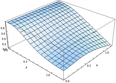
Figure 1: Surfaces of $\eta(\sqrt{R_{e}},y,z)$ and $\zeta(\sqrt{R_{e}},y,z)$ over the domain $(0,\sqrt{R_{e}})^{2}$.

Lemma A.2.

For the function $p$ defined by (3.14) for $0<x,y,z<R_{e}$, it holds that

$$p= \,2d_{0}(y,z)+\frac{7}{10}\sqrt{y}d_{1}(y,z)-\frac{51}{100}\sqrt{yz}d_{2}(y,z)+\frac{10}{7}\sqrt{x}d_{1}(x,y)+\sqrt{xy}d_{2}(x,y)>\frac{1}{50}.$$

Proof.

Reminding the function $d_{*}$ defined by (3.12), we consider an auxiliary function

$$\zeta(x,y,z):=\frac{\zeta_{1}(y,z)+\zeta_{2}(x,y)}{1+y^{2}}\quad\text{for $0<x,y,z<\sqrt{R_{e}}$},$$

where

$$\zeta_{1}(y,z):= \,2d_{0}(y^{2},z^{2})+\frac{7}{10}yd_{1}(y^{2},z^{2})-\frac{51}{100}yzd_{2}(y^{2},z^{2}),$$

$$\zeta_{2}(x,y):= \,-d_{*}(x^{2},y^{2})=\frac{10}{7}xd_{1}(x^{2},y^{2})+xyd_{2}(x^{2},y^{2}).$$

Obviously, one has

$$p(x^{2},y^{2},z^{2})=\zeta_{1}(y,z)+\zeta_{2}(x,y)=\zeta(x,y,z)(1+y^{2})\quad\text{for $0<x,y,z<\sqrt{R_{e}}$.}$$ (A.6)

At first we examine the function $\zeta(x,y,z).$ It is not difficult to show that

$$\zeta_{2}(x,y)=-\frac{10x^{3}}{7\left(x^{2}+1\right)}-\frac{x^{3}y^{2}(10-7y)}{7\left(y^{2}+1\right)}-\frac{(10y+7)y^{3}}{7\left(y^{2}+1\right)}\frac{x^{3}}{1+y^{2}+y^{2}x^{2}}.$$

Since $x^{3}/(c_{1}+c_{2}x^{2})$ ($c_{1}>0$ and $c_{2}\geq 0$ are constants) is increasing with respect to $x$, the function $\zeta_{2}$ and $\zeta$ are decreasing with respect to $x$ so that

$$\zeta(x,y,z)>\zeta(\sqrt{R_{e}},y,z)\quad\text{for $0<x,y,z<\sqrt{R_{e}}$}.$$ (A.7)

By following the elementary arguments in (A.3)-(A.5), one can verify that $\frac{\partial}{\partial y}\zeta(\sqrt{R_{e}},y,z)<0$; but the tediously long detials are omitted here. As depicted in Figure 1 (b), $\zeta(\sqrt{R_{e}},y,z)$ has no any extreme points in $(0,R_{3})^{2}$. We consider the minimum value along the four boundaries:

• Along the side $y=0$, we have $\zeta(\sqrt{R_{e}},0,z)=2-10R_{e}\sqrt{R_{e}}/(7+7R_{e})\approx 0.9579$.

• Along the side $y=\sqrt{R_{e}}$,

  $$\zeta(\sqrt{R_{e}},\sqrt{R_{e}},z)\approx \,\frac{-0.372002z^{5}+0.0240772z^{4}+0.638833z^{2}+0.104165}{z^{4}+1.40198z^{2}+0.401978}.$$

  It has a unique maximum point at $z_{3}^{*}\approx 0.448068$ and then

  $$\zeta(\sqrt{R_{e}},\sqrt{R_{e}},z)> \,\min\left\{\zeta(\sqrt{R_{e}},\sqrt{R_{e}},0),\zeta(\sqrt{R_{e}},\sqrt{R_{e}},z_{3}^{*}),\zeta(\sqrt{R_{e}},\sqrt{R_{e}},\sqrt{R_{e}})\right\}$$

  $$= \,\zeta(\sqrt{R_{e}},\sqrt{R_{e}},\sqrt{R_{e}})>\frac{1}{50}\qquad\text{for $0<z<\sqrt{R_{e}}$.}$$

• Along the side $z=0$, we have

  $$\zeta(\sqrt{R_{e}},y,0)\approx \,\frac{1.11457y^{5}-0.676283y^{4}-0.281384y^{3}+1.105y^{2}+0.385086}{\left(y^{2}+1\right)^{2}\left(y^{2}+0.401978\right)}.$$

  It is decreasing such that $\zeta(\sqrt{R_{e}},y,0)>\zeta(\sqrt{R_{e}},\sqrt{R_{e}},0)\approx 0.259131$ for $0<y<\sqrt{R_{e}}$.

• Along the side $z=\sqrt{R_{e}}$, one has

  $$\zeta(\sqrt{R_{e}},y,\sqrt{R_{e}})\approx \,\frac{\left(y^{2}+1\right)^{-2}}{y^{4}+2.07416y^{2}+0.672179}\Big{(}-0.790618y^{9}-1.48448y^{7}+1.32372y^{6}\Big{.}$$

  $$\,\Big{.}-0.825252y^{5}+2.77809y^{4}-1.06972y^{3}+3.03679y^{2}+0.643932\Big{)}.$$

  It is also decreasing such that

  $$\zeta(\sqrt{R_{e}},y,\sqrt{R_{e}})>\zeta(\sqrt{R_{e}},\sqrt{R_{e}},\sqrt{R_{e}})>\frac{1}{50}\quad\text{for $0<y<\sqrt{R_{e}}$.}$$

It follows from (A.7) that $\zeta(x,y,z)>\frac{1}{50}$ for $0<x,y,z<\sqrt{R_{e}}$. According to (A.6), we have $p(x^{2},y^{2},z^{2})>\frac{1+y^{2}}{50}$ for $0<x,y,z<\sqrt{R_{e}}$. This completes the proof. ∎

References

- [1] G. Albi, G. Dimarco and L. Pareschi, Implicit-explicit multistep methods for hyperbolic systems with multiscale relaxation, SIAM J. Sci. Comput., 42(4), A2402–A2435 (2020).
- [2] M. Calvo, T. Grande and R. D. Grigorieff, On the zero stability of the variable order variable stepsize BDF-formulas, Numer. Math., 57, 39–50 (1990).
- [3] M. Calvo and R. D. Grigorieff, Time discretisation of parabolic problems with the variable 3-step BDF, BIT, 42, 689-701 (2002).
- [4] W. Chen, X. Wang, Y. Yan and Z. Zhang, A second order BDF numerical scheme with variable steps for the Cahn–Hilliard equation, SIAM J. Numer. Anal., 57 (1) (2019), 495–525.
- [5] G. Dimarco and L. Pareschi, Implicit-explicit linear multistep methods for stiff kinetic equations, SIAM J. Numer. Anal., 55, 664–690 (2017).
- [6] V. DeCaria, A. Guzel, W. Layton and Y. Li, A variable stepsize, variable order family of low complexity, SIAM J. Sci. Comput., 43 (3), A2130-A2160 (2021).
- [7] E. Hairer, S. P. Nørsett and G. Wanner, Solving Ordinary Differential Equations I: Nonstiff Problems, Volume 8 of Springer Series in Computational Mathematics, Second Edition, Springer-Verlag, 1992.
- [8] E. Hairer and G. Wanner, Solving Ordinary Differential Equations II: Stiff and Differential-Algebraic Problems, Springer Series in Computational Mathematics Volume 14, Second Edition, Springer-Verlag, 2002.
- [9] Z. Li and H.-L. Liao, Stability of variable-step BDF2 and BDF3 methods, arXiv:2201.00527, 2021, submitted.
- [10] H.-L. Liao, B. Ji and L. Zhang, An adaptive BDF2 implicit time-stepping method for the phase field crystal model, IMA J. Numer. Anal., 42(1), 649–679 (2022).
- [11] H.-L. Liao, T. Tang and T. Zhou, On energy stable, maximum-bound preserving, second-order BDF scheme with variable steps for the Allen-Cahn equation, SIAM J. Numer. Anal., 58(4), 2294-2314 (2020).
- [12] H.-L. Liao, T. Tang and T. Zhou, A new discrete energy technique for multi-step backward difference formulas, CSIAM Trans. Appl. Math., 2022, doi: 10.4208/csiam-am.SO-2021-0032.
- [13] H.-L. Liao and Z. Zhang, Analysis of adaptive BDF2 scheme for diffusion equations, Math. Comp., 90, 1207–1226 (2021).
- [14] M. Pierre, Maximum time step for the BDF3 scheme applied to gradient flows, Calcolo, 58 (2021), doi:10.1007/s10092-020-00393-3.
- [15] A.M. Stuart and A.R. Humphries, Dynamical systems and numerical analysis, Cambridge University Press, New York, 1998.
- [16] D. Wang and S. T. Ruuth, Variable step-size implicit-explicit linear multistep methods for time-dependent partial differential equations, J. Comput. Math., 26(6), 838–855 (2008).