NNLO+PS Monte Carlo simulation of photon pair production with MiNNLO_PS

Abstract

We present a NNLO QCD accurate event generator for direct photon pair production at hadron colliders, based on the MiNNLO_PS formalism, within the Powheg Box Res framework. Despite the presence of the photons requires the use of isolation criteria, our generator is built such that no technical cuts are needed at any stage of the event generation. Therefore, our predictions can be used to simulate kinematic distributions with arbitrary fiducial cuts. Furthermore, we describe a few modifications of the MiNNLO_PS formalism in order to allow for a setting of the renormalization and factorization scales more similar to that of a fixed-order computation, thus reducing the numerical impact of higher-order terms beyond the nominal accuracy. Finally, we show several phenomenological distributions of physical interest obtained by showering the generated events with Pythia8, and we compare them with the 13 TeV data from the ATLAS Collaboration.

1 Introduction

The production of two isolated photons at hadron colliders, henceforth denoted diphoton production and abbreviated as $pp\rightarrow\gamma\gamma$, is one among the most relevant Standard Model (SM) processes, due, on one side, to the high production rate, and, on the other, to the relative cleanliness of the experimental final state. Furthermore, diphoton production is the dominant background for studies involving Higgs boson production decaying into a photon pair, and, notably, it was one of the dominant backgrounds for the Higgs boson discovery ATLAS:2012yve ; CMS:2012qbp at the Large Hadron Collider (LHC). In addition, it is a background for searches for heavy neutral resonances that can arise in a variety of beyond the Standard Model scenarios (see e.g. Mrenna:2000qh ; Han:1998sg ; Giudice:1998bp ; Giudice:2017fmj ), and for searches for extra dimensions or supersymmetry, and a possible channel for their detection ATLAS:2017ayi ; CMS:2018dqv .

Within the SM, photon pairs can be produced by means of several mechanisms, that make this otherwise simple process particularly challenging to study. In this work we restrict to prompt photon production, where photons are produced in the hard process. Within this category, one can further distinguish two components: one arising from direct photon production and the other from single and double fragmentation. In the former case, the photons are directly produced in the hard scattering, whereas, in the latter case, one or both photons are produced through the fragmentation of jets. The latter mechanism can be suppressed by imposing the isolation of the photons from the hadronic activity through a fixed or a smooth cone algorithm Frixione:1998jh . In spite of the fact that the fixed-cone isolation criterion is simpler to apply (also at the experimental level), only the smooth-cone isolation is suitable for theoretical calculations, as it allows to completely remove the fragmentation component in an infrared-safe way.

Theoretical predictions for diphoton direct production at next-to-leading-order (NLO) QCD accuracy, that consistently include also the fragmentation component, were obtained for the first time in ref. Binoth:1999qq , and made publicly available in the DIPHOX software. Next-to-next-to-leading-order (NNLO) QCD corrections to $pp\rightarrow\gamma\gamma$ were obtained in refs. Catani:2011qz ; Campbell:2016yrh ; Catani:2018krb ; Gehrmann:2020oec , whereas NLO electroweak corrections have been studied in ref. Bierweiler:2013dja . More recently, even the three-loop $q\bar{q}\rightarrow\gamma\gamma$ amplitudes have been computed Caola:2020dfu . In order to include all the effects up to $\alpha_{\mathchoice{\displaystyle}{\scriptstyle}{\scriptscriptstyle}{\scriptscriptstyle}\rm S}^{2}$ accuracy, the gluon-induced production of a photon pair through a closed quark loop has to be taken into account as well: such contribution, that is particularly sizable due to the gluon luminosity, was first computed in ref. Dicus:1987fk , and it is by now known at the next order, both for massless Bern:2002jx and for massive quark loops Maltoni:2018zvp ; Chen:2019fla . Substantial progress has also been made for the computation of a photon pair in association with one or more jets: predictions for diphoton in association with up to three jets, including NLO QCD corrections, have been obtained in refs. DelDuca:2003uz ; Gehrmann:2013aga ; Gehrmann:2013bga ; Badger:2013ava , and NLO electroweak (EW) corrections for photon pair with up to two jets are also known Chiesa:2017gqx . Very recently, the NNLO QCD results for $pp\rightarrow\gamma\gamma+j$ were obtained as well Chawdhry:2021hkp ; Agarwal:2021vdh ; Agarwal:2021grm , and the two-loop amplitudes for $gg\rightarrow\gamma\gamma+j$ Badger:2021imn were also computed. Finally, as far as all-order results are concerned, Sudakov logarithms of soft and collinear origin, arising at all orders in the computation of the diphoton transverse-momentum distribution, were resummed up to next-to-next-to-leading-logarithmic (NNLL) accuracy in refs. Balazs:2006cc ; Nadolsky:2007ba ; Balazs:2007hr ; Cieri:2015rqa ; Coradeschi:2017zzw . More recently, results accurate up to N³LL and N³LL^′ have also been obtained within the RadISH formalism Monni:2016ktx ; Bizon:2017rah and the CuTe-MCFM framework Becher:2020ugp ; Neumann:2021zkb , respectively.

Nowadays, NLO Monte Carlo simulations for $pp\rightarrow\gamma\gamma$, matched to parton showers (PS), can be easily obtained with automated tools. A few dedicated studies have been presented in the last decade: for instance, in ref. Hoeche:2009xc , hard tree-level matrix elements with a variable photon multiplicity were merged with a QCD+EW parton shower, allowing to take simultaneously into account the direct and the fragmentation component. In ref. DErrico:2011cgc these two components were also included in the simulation, in the context of an exact matching of the NLO QCD corrections with parton showers (NLO+PS), using the Powheg method Nason:2004rx .

Due to the increasing precision of experimental measurements and the fact that NNLO QCD corrections to photon-pair production are known and sizable, it is particularly important to match parton showers with the NNLO fixed order calculation (NNLO+PS). A few methods have been developed to obtain NNLO+PS predictions for color-singlet production at hadron colliders: “NNLO reweighted” MiNLO^′ Hamilton:2012rf ; Hamilton:2013fea (sometimes also denoted NNLOPS in the literature), Geneva Alioli:2012fc ; Alioli:2013hqa , UN²LOPS Hoche:2014uhw , and MiNNLO_PS Monni:2019whf ; Monni:2020nks . Using these methods, many processes, that at leading order (LO) have only two external colored legs, have been described with NNLO+PS accuracy Hamilton:2013fea ; Karlberg:2014qua ; Astill:2016hpa ; Astill:2018ivh ; Re:2018vac ; Bizon:2019tfo ; Alioli:2015toa ; Alioli:2019qzz ; Alioli:2020fzf ; Alioli:2020qrd ; Alioli:2021qbf ; Alioli:2021egp ; Cridge:2021hfr ; Hoche:2014uhw ; Hoche:2014dla ; Hoche:2018gti ; Monni:2019whf ; Monni:2020nks ; Lombardi:2020wju ; Lombardi:2021rvg ; Hu:2021rkt ; Buonocore:2021fnj . Recently, results for top-pair production at NNLO+PS were also published in ref. Mazzitelli:2020jio ; Mazzitelli:2021mmm . As far as diphoton production is concerned, the only NNLO+PS accurate results have been obtained with the Geneva method in ref. Alioli:2020qrd .

In this paper we study diphoton production using the MiNNLO_PS method, i.e. we build a MiNLO^′ simulation for $pp\rightarrow\gamma\gamma$ + jet production, and we subsequently include NNLO QCD corrections according to the procedure proposed in refs. Monni:2019whf ; Monni:2020nks . The resulting generator can be used to obtain NLO+PS accurate results for $\gamma\gamma j$ production, as well as to predict, with up to NNLO accuracy, observables that are inclusive with respect to the presence of jets, such as the diphoton invariant mass and rapidity, or the transverse momentum of the hardest and next-to-hardest photon, retaining a consistent matching with parton showers.

Together with the main phenomenological results for diphoton production, in the current paper we also describe a few novelties introduced to deal with the presence of photons in the final state, but that could also be useful for other (N)NLO+PS calculations. First of all, already for the simulation of diphoton + jet production at NLO+PS accuracy, one needs to deal with the fact that the Born-level $\gamma\gamma j$ matrix elements are divergent whenever a photon becomes soft or collinear to a quark. In the following, we refer to these divergences as “QED divergences”. We describe and implement a general way to deal with this issue in the Powheg formalism. Furthermore, the MiNNLO_PS method for the process at hand requires the evaluation of the $q\bar{q}\rightarrow\gamma\gamma$ matrix-elements up to second order in the strong coupling constant. Such matrix elements are divergent when the photons are collinear to the beam axis: in order to avoid introducing any cutoff or isolation criteria at any stage of the event generation, we have also devised a new mapping from the $pp\rightarrow\gamma\gamma+j$ to the $pp\rightarrow\gamma\gamma$ kinematics, that preserves the direction of one photon with respect to the beam axis, thereby allowing for a full control of the singular regions. The combined use of the new mapping and of the method to deal with the QED divergences allowed us to simulate diphoton production at NNLO+PS accuracy without introducing any generation or technical cut, as done instead in refs. Lombardi:2020wju ; Alioli:2020qrd . This gives us the advantage that, on one side, we do not have to worry about checking the independence of the fiducial physical differential cross sections from the generation and technical cuts, and, on the other side, we can use the same set of generated events for any choice of fiducial cuts.

In this paper we also propose a generalization of the MiNNLO_PS method that allows for greater flexibility in the choice of the renormalization and factorization scale used in the evaluation of the non-singular term for $F$ + 1 jet production, where $F$ is the color-singlet system. In the original formulation of the MiNNLO_PS method, such term is evaluated with scales of the order of the transverse momentum of $F$. The prescription we introduce here generalizes such aspect of the MiNNLO_PS method, allowing one to treat this term more similarly to a fixed-order computation. Such choice turned out to be desirable in $\gamma\gamma$ production, for comparisons with fixed-order results, where this term gives an important contribution to the total cross section, unlike in previous studies, such as those in refs. Monni:2019whf ; Monni:2020nks , where it was small.

The paper is organized as follows: in section 2 we describe the ingredients used to build the event generator and the details of the novel aspects we introduce here for the first time, whose validation is discussed in section 3. In section 4 we show some phenomenological results, and we compare our predictions with the ATLAS diphoton data ATLAS:2021mbt . Finally we give our conclusions and outlook in section 5.

2 Outline of the calculation

In this section we review the theoretical formulation of our calculation. We first introduce the basic notation used throughout the paper and describe the main theoretical issues to be dealt with in the implementation of a NNLO+PS event generator for photon pair production. Then we discuss in detail the handling of the QED singularities and introduce the mapping used to project the $\Phi_{\gamma\gamma j}$ kinematics onto the $\Phi_{\mathchoice{\displaystyle}{\scriptstyle}{\scriptscriptstyle}{\scriptscriptstyle}\gamma\gamma}$ one. We conclude the section with a description of the modifications we have introduced in the MiNNLO_PS formalism in order to reproduce more accurately the results of a fixed-order calculation for distributions totally inclusive with respect to the QCD radiation.

2.1 Description of the process

We consider the process of direct production of a photon pair in proton-proton scattering

$$pp\,\rightarrow\,\gamma\gamma+X,$$ (1)

with the requirement that the two photons are isolated, i.e. each photon has a minimum transverse momentum and is isolated with respect to the other photon and to the final-state hadronic activity. These requirements are needed to make the process well-defined both from the theoretical and the experimental point of view. We call $p_{\gamma_{1}}$ and $p_{\gamma_{2}}$ the momenta of the hardest and next-to-hardest photons and denote the squared mass and transverse momentum of the diphoton system as

$$Q^{2}=m_{\gamma\gamma}^{2}=\left(p_{\gamma_{1}}+p_{\gamma_{2}}\right)^{2}\!,\qquad\qquad p_{\mathchoice{\displaystyle}{\scriptstyle}{\scriptscriptstyle}{\scriptscriptstyle}\rm T}=\left(p_{\gamma_{1}}+p_{\gamma_{2}}\right)_{\mathchoice{\displaystyle}{\scriptstyle}{\scriptscriptstyle}{\scriptscriptstyle}\rm T}.$$ (2)

The starting point for the MiNNLO_PS method we use in this work is the NLO differential cross section for diphoton plus one jet production

$$pp\,\rightarrow\,\gamma\gamma+j\,.$$ (3)

The matrix elements for this process at NLO in QCD have been obtained from the automated interface of the Powheg Box Res Jezo:2016ujg to OpenLoops2 Buccioni:2019sur ; Cascioli:2011va ; Buccioni:2017yxi ; vanHameren:2010cp ; vanHameren:2009dr .

Since the goal of the MiNNLO_PS formalism is to reach NNLO accuracy for inclusive observables in the diphoton system, one also needs the two-loop amplitudes for $q\bar{q}\rightarrow\gamma\gamma$, that have been taken from refs. Anastasiou:2002zn ; Catani:2013tia and implemented into the code.

In this paper, we work in the approximation of five light quarks and neglect the contributions given by two-loop diagrams with the massive top quark. We consider instead the contributions given by the massive top quark in the one-loop diagrams for the process $pp\rightarrow\gamma\gamma+j$.

2.2 Handling of the QED divergences

In this section, we describe a general way to deal with processes that present QED divergences at the Born level within the Powheg formalism. Before illustrating the method, we briefly review the relevant parts of the Powheg Box framework.

We start by introducing the general form of the Powheg Nason:2004rx differential cross section for a $2\rightarrow n$ Born process, using the notation of refs. Frixione:2007vw ; Alioli:2010xd . Indicating with $\mathrm{d}{\Phi}_{n}$ the phase space for the $n$-body final state, we write the $(n+1)$-body phase space $\mathrm{d}{\Phi}_{n+1}$ in terms of $\mathrm{d}{\Phi}_{n}$ and three additional radiation variables, that we collectively label $\Phi_{\mathchoice{\displaystyle}{\scriptstyle}{\scriptscriptstyle}{\scriptscriptstyle}{\rm rad}}$

$$\mathrm{d}{\Phi}_{n+1}=\mathrm{d}{\Phi}_{n}\,\mathrm{d}\Phi_{\mathchoice{\displaystyle}{\scriptstyle}{\scriptscriptstyle}{\scriptscriptstyle}{\rm rad}}\,.$$ (4)

We indicate with $B({\Phi}_{n})$, $V({\Phi}_{n})$ and $R({\Phi}_{n+1})$ the Born, virtual and real amplitudes, convoluted with the corresponding parton distribution functions (PDFs) and multiplied by the flux factor, and we split $R$ into two positive contributions: $R_{s}({\Phi}_{n+1})$, that contains all the QCD singularities, and a QCD-finite term, $R_{f}({\Phi}_{n+1})$, such that

$$R({\Phi}_{n+1})=R_{s}({\Phi}_{n+1})+R_{f}({\Phi}_{n+1}).$$ (5)

In general we achieve this separation with the help of a suitable function $F({\Phi}_{n+1})$, such that

$$R_{s}({\Phi}_{n+1})=F({\Phi}_{n+1})\,R({\Phi}_{n+1})\,,\qquad\qquad R_{f}({\Phi}_{n+1})=\left[1-F({\Phi}_{n+1})\right]R({\Phi}_{n+1})\,.$$ (6)

The detailed form for $F({\Phi}_{n+1})$ will be discussed in section 2.2.1. When $R({\Phi}_{n+1})$ is split as in eq. (5), the Powheg differential cross section can be written as

$$\mathrm{d}\sigma = \bar{B}\!\left({\Phi}_{n}\right)\!\left\{\Delta\!\left({\Phi}_{n},k_{\mathchoice{\displaystyle}{\scriptstyle}{\scriptscriptstyle}{\scriptscriptstyle}\rm T}^{\rm\mathchoice{\displaystyle}{\scriptstyle}{\scriptscriptstyle}{\scriptscriptstyle}min}\right)+\theta\!\left({k_{\rm\mathchoice{\displaystyle}{\scriptstyle}{\scriptscriptstyle}{\scriptscriptstyle}T}}-k_{\mathchoice{\displaystyle}{\scriptstyle}{\scriptscriptstyle}{\scriptscriptstyle}\rm T}^{\rm\mathchoice{\displaystyle}{\scriptstyle}{\scriptscriptstyle}{\scriptscriptstyle}min}\right)\Delta\!\left({\Phi}_{n},{k_{\rm\mathchoice{\displaystyle}{\scriptstyle}{\scriptscriptstyle}{\scriptscriptstyle}T}}\right)\,\frac{{R_{s}\!\left({\Phi}_{n+1}\right)}}{B\!\left({\Phi}_{n}\right)}\,\,\mathrm{d}\Phi_{\mathchoice{\displaystyle}{\scriptstyle}{\scriptscriptstyle}{\scriptscriptstyle}{\rm rad}}\right\}\mathrm{d}{\Phi}_{n}$$ (7)

$${}+R_{f}\!\left({\Phi}_{n+1}\right)\mathrm{d}{\Phi}_{n+1}\,,$$

where ${k_{\rm\mathchoice{\displaystyle}{\scriptstyle}{\scriptscriptstyle}{\scriptscriptstyle}T}}$ is the transverse momentum of the Powheg jet,

$$\bar{B}({\Phi}_{n})=B({\Phi}_{n})+V({\Phi}_{n})+\int\mathrm{d}\Phi_{\mathchoice{\displaystyle}{\scriptstyle}{\scriptscriptstyle}{\scriptscriptstyle}{\rm rad}}\,{R_{s}({\Phi}_{n},\Phi_{\mathchoice{\displaystyle}{\scriptstyle}{\scriptscriptstyle}{\scriptscriptstyle}{\rm rad}})}\,,$$ (8)

and the Powheg Sudakov form factor

$$\Delta\!\left({\Phi}_{n},{k_{\rm\mathchoice{\displaystyle}{\scriptstyle}{\scriptscriptstyle}{\scriptscriptstyle}T}}\right)=\exp\left\{-\int\mathrm{d}\Phi_{\mathchoice{\displaystyle}{\scriptstyle}{\scriptscriptstyle}{\scriptscriptstyle}{\rm rad}}^{\prime}\,{\frac{{R_{s}({\Phi}_{n},\Phi_{\mathchoice{\displaystyle}{\scriptstyle}{\scriptscriptstyle}{\scriptscriptstyle}{\rm rad}}^{\prime})}}{B({\Phi}_{n})}}\,\theta\!\left[{k_{\rm\mathchoice{\displaystyle}{\scriptstyle}{\scriptscriptstyle}{\scriptscriptstyle}T}}^{\prime}\!\left({\Phi}_{n},\Phi_{\mathchoice{\displaystyle}{\scriptstyle}{\scriptscriptstyle}{\scriptscriptstyle}{\rm rad}}^{\prime}\right)-{k_{\rm\mathchoice{\displaystyle}{\scriptstyle}{\scriptscriptstyle}{\scriptscriptstyle}T}}\right]\right\}$$ (9)

contains only the QCD singular part of the real contributions $R_{s}({\Phi}_{n+1})$. In the expressions above $k_{\mathchoice{\displaystyle}{\scriptstyle}{\scriptscriptstyle}{\scriptscriptstyle}\rm T}^{\rm\mathchoice{\displaystyle}{\scriptstyle}{\scriptscriptstyle}{\scriptscriptstyle}min}$ acts as an infrared cutoff for unresolved radiation.

If the Born amplitude is divergent, the Powheg Box applies a suppression factor ${S_{\mathchoice{\displaystyle}{\scriptstyle}{\scriptscriptstyle}{\scriptscriptstyle}\rm B}}({\Phi}_{n})$ to $\bar{B}({\Phi}_{n})$ such that the product ${S_{\mathchoice{\displaystyle}{\scriptstyle}{\scriptscriptstyle}{\scriptscriptstyle}\rm B}}({\Phi}_{n})\bar{B}({\Phi}_{n})$ is integrable over the entire Born phase space, and the ${\Phi}_{n}$ kinematics can be generated from the distribution ${S_{\mathchoice{\displaystyle}{\scriptstyle}{\scriptscriptstyle}{\scriptscriptstyle}\rm B}}({\Phi}_{n})\bar{B}({\Phi}_{n})$ without the need of any hard cut. At the end, each event is given a weight $1/{S_{\mathchoice{\displaystyle}{\scriptstyle}{\scriptscriptstyle}{\scriptscriptstyle}\rm B}}({\Phi}_{n})$ in order to compensate for the suppression factor.

In general, this way of regularizing divergences by means of a suppression factor that depends on ${\Phi}_{n}$ can be used every time QCD and/or QED singularities are present at the Born level. While applying a suppression factor on $\bar{B}({\Phi}_{n})$ is enough when only QCD singularities are present, for diphoton production we also have to deal with the QED singularities appearing inside $R_{f}({\Phi}_{n+1})$. We cannot simply suppress them through a second suppression factor (that would be a function of ${\Phi}_{n+1}$) since this term is integrated in the radiation variables inside $\bar{B}({\Phi}_{n})$, preventing one to compensate for such suppression factor, after the events have been generated.

We then proceed as follows: we take advantage of the possibility to separate the real contributions into two terms (see eq. (5)) in such a way that $R_{s}({\Phi}_{n+1})$ contains all the QCD singularities but no QED ones. Since the generation of ${\Phi}_{n+1}$ according to $R_{f}({\Phi}_{n+1})$ in eq. (7) is performed with a hit-and-miss technique, we apply a QED suppression factor ${S_{\mathchoice{\displaystyle}{\scriptstyle}{\scriptscriptstyle}{\scriptscriptstyle}\rm R}}({\Phi}_{n+1})$ to $R_{f}({\Phi}_{n+1})$, and generate ${\Phi}_{n+1}$ according to the product ${S_{\mathchoice{\displaystyle}{\scriptstyle}{\scriptscriptstyle}{\scriptscriptstyle}\rm R}}({\Phi}_{n+1})R_{f}({\Phi}_{n+1})$, that is now integrable. Finally, we multiply the weights of the generated events by the factor $1/{S_{\mathchoice{\displaystyle}{\scriptstyle}{\scriptscriptstyle}{\scriptscriptstyle}\rm R}}({\Phi}_{n+1})$.

2.2.1 The damping function $\boldsymbol{F}$

According to the FKS method Frixione:1995ms ; Frixione:1997np , the real contribution $R$ is partitioned into a sum of terms $R^{{\alpha_{\rm\mathchoice{\displaystyle}{\scriptstyle}{\scriptscriptstyle}{\scriptscriptstyle}r}}}$, each of them having at most one collinear and one soft singularity associated with one parton

$$R=\sum_{{\alpha_{\rm\mathchoice{\displaystyle}{\scriptstyle}{\scriptscriptstyle}{\scriptscriptstyle}r}}}R^{\alpha_{\rm\mathchoice{\displaystyle}{\scriptstyle}{\scriptscriptstyle}{\scriptscriptstyle}r}}\,.$$ (10)

In each ${\alpha_{\rm\mathchoice{\displaystyle}{\scriptstyle}{\scriptscriptstyle}{\scriptscriptstyle}r}}$ region, the radiated parton (r) can then become soft or be collinear to an emitting one (e), and we can define the damping function

$$F^{\alpha_{\rm\mathchoice{\displaystyle}{\scriptstyle}{\scriptscriptstyle}{\scriptscriptstyle}r}}=\frac{\left(\frac{\displaystyle 1}{\displaystyle d_{\rm\mathchoice{\displaystyle}{\scriptstyle}{\scriptscriptstyle}{\scriptscriptstyle}e,r}}\right)^{p}}{\displaystyle\left(\frac{\displaystyle 1}{\displaystyle d_{\rm\mathchoice{\displaystyle}{\scriptstyle}{\scriptscriptstyle}{\scriptscriptstyle}e,r}}\right)^{p}+\sum_{i=1}^{n_{\rm c}}\sum_{j=1}^{n_{\gamma}}\left(\frac{1}{d_{c_{i},\gamma_{j}}}\right)^{p}}\,,$$ (11)

where

$$d_{i,j}=\left\{\begin{array}[]{l l}\displaystyle p_{{\mathchoice{\displaystyle}{\scriptstyle}{\scriptscriptstyle}{\scriptscriptstyle}\rm T}j}^{2}&\mbox{if $i$ is an initial-state particle,}\\[5.69054pt] \displaystyle 2\min\!\left(E_{i}^{2},E_{j}^{2}\right)\left(1-\cos\theta_{ij}\right)&\mbox{if $i$ and $j$ are final-state particles,}\end{array}\right.$$ (12)

and the sum in the denominator runs over the $n_{\mathchoice{\displaystyle}{\scriptstyle}{\scriptscriptstyle}{\scriptscriptstyle}\rm c}$ massless charged particles and the $n_{\gamma}$ photons. In eq. (12), $p_{{\mathchoice{\displaystyle}{\scriptstyle}{\scriptscriptstyle}{\scriptscriptstyle}\rm T}j}$ and $E_{j}$ are the transverse momentum and energy of the particle $j$, and $\theta_{ij}$ the angle between the particles $i$ and $j$, computed in the partonic center-of-mass frame.

Every contribution $R^{\alpha_{\rm\mathchoice{\displaystyle}{\scriptstyle}{\scriptscriptstyle}{\scriptscriptstyle}r}}$ to the real amplitude is then split into two terms

$$R^{{\alpha_{\rm\mathchoice{\displaystyle}{\scriptstyle}{\scriptscriptstyle}{\scriptscriptstyle}r}}}=R^{{\alpha_{\rm\mathchoice{\displaystyle}{\scriptstyle}{\scriptscriptstyle}{\scriptscriptstyle}r}}}_{s}+R^{{\alpha_{\rm\mathchoice{\displaystyle}{\scriptstyle}{\scriptscriptstyle}{\scriptscriptstyle}r}}}_{f}\,,$$ (13)

where

$$R^{{\alpha_{\rm\mathchoice{\displaystyle}{\scriptstyle}{\scriptscriptstyle}{\scriptscriptstyle}r}}}_{s}\equiv F^{{\alpha_{\rm\mathchoice{\displaystyle}{\scriptstyle}{\scriptscriptstyle}{\scriptscriptstyle}r}}}R^{{\alpha_{\rm\mathchoice{\displaystyle}{\scriptstyle}{\scriptscriptstyle}{\scriptscriptstyle}r}}},\qquad\qquad\qquad R^{{\alpha_{\rm\mathchoice{\displaystyle}{\scriptstyle}{\scriptscriptstyle}{\scriptscriptstyle}r}}}_{f}\equiv\left(1-F^{{\alpha_{\rm\mathchoice{\displaystyle}{\scriptstyle}{\scriptscriptstyle}{\scriptscriptstyle}r}}}\right)R^{\alpha_{\rm\mathchoice{\displaystyle}{\scriptstyle}{\scriptscriptstyle}{\scriptscriptstyle}r}}\,.$$ (14)

In the limit where the radiated parton is soft or collinear to the emitter $d_{\rm\mathchoice{\displaystyle}{\scriptstyle}{\scriptscriptstyle}{\scriptscriptstyle}e,r}$ is small, and $F^{{\alpha_{\rm\mathchoice{\displaystyle}{\scriptstyle}{\scriptscriptstyle}{\scriptscriptstyle}r}}}$ tends to 1, so that all the QCD singularities are in $R^{{\alpha_{\rm\mathchoice{\displaystyle}{\scriptstyle}{\scriptscriptstyle}{\scriptscriptstyle}r}}}_{\mathchoice{\displaystyle}{\scriptstyle}{\scriptscriptstyle}{\scriptscriptstyle}\rm s}$. When instead the photon $\gamma_{j}$ becomes soft or collinear to a massless charged particle $c_{i}$, the term $d_{c_{i},\gamma_{j}}$ is small, and $F^{{\alpha_{\rm\mathchoice{\displaystyle}{\scriptstyle}{\scriptscriptstyle}{\scriptscriptstyle}r}}}$ tends to 0, so that $R^{{\alpha_{\rm\mathchoice{\displaystyle}{\scriptstyle}{\scriptscriptstyle}{\scriptscriptstyle}r}}}_{\mathchoice{\displaystyle}{\scriptstyle}{\scriptscriptstyle}{\scriptscriptstyle}\rm s}$ is free from QED singularities.

2.2.2 The suppression factors $\boldsymbol{{S_{\mathchoice{\displaystyle}{\scriptstyle}{\scriptscriptstyle}{\scriptscriptstyle}\rm B}}}$ and $\boldsymbol{{S_{\mathchoice{\displaystyle}{\scriptstyle}{\scriptscriptstyle}{\scriptscriptstyle}\rm R}}}$

We have chosen as suppression factor ${S_{\mathchoice{\displaystyle}{\scriptstyle}{\scriptscriptstyle}{\scriptscriptstyle}\rm B}}({\Phi}_{n})$ introduced in section 2.2 the following expression

$${S_{\mathchoice{\displaystyle}{\scriptstyle}{\scriptscriptstyle}{\scriptscriptstyle}\rm B}} = \frac{\left(p^{2}_{{\mathchoice{\displaystyle}{\scriptstyle}{\scriptscriptstyle}{\scriptscriptstyle}\rm T}j}\right)^{a}}{\left(p^{2}_{{\mathchoice{\displaystyle}{\scriptstyle}{\scriptscriptstyle}{\scriptscriptstyle}\rm T}j}\right)^{a}+\left(\bar{p}^{2}_{{\mathchoice{\displaystyle}{\scriptstyle}{\scriptscriptstyle}{\scriptscriptstyle}\rm T}j}\right)^{a}}\,\frac{\left(p^{2}_{{\mathchoice{\displaystyle}{\scriptstyle}{\scriptscriptstyle}{\scriptscriptstyle}\rm T}\gamma_{1}}\right)^{a}}{\left(p^{2}_{{\mathchoice{\displaystyle}{\scriptstyle}{\scriptscriptstyle}{\scriptscriptstyle}\rm T}\gamma_{1}}\right)^{a}+\left(\bar{p}^{2}_{{\mathchoice{\displaystyle}{\scriptstyle}{\scriptscriptstyle}{\scriptscriptstyle}\rm T}\gamma}\right)^{a}}\,\frac{\left(p^{2}_{{\mathchoice{\displaystyle}{\scriptstyle}{\scriptscriptstyle}{\scriptscriptstyle}\rm T}\gamma_{2}}\right)^{a}}{\left(p^{2}_{{\mathchoice{\displaystyle}{\scriptstyle}{\scriptscriptstyle}{\scriptscriptstyle}\rm T}\gamma_{2}}\right)^{a}+\left(\bar{p}^{2}_{{\mathchoice{\displaystyle}{\scriptstyle}{\scriptscriptstyle}{\scriptscriptstyle}\rm T}\gamma}\right)^{a}}$$ (15)

$${}\times\frac{\left(R^{2}_{j\gamma_{1}}\right)^{a}}{\left(R^{2}_{j\gamma_{1}}\right)^{a}+\left(\bar{R}^{2}_{j\gamma}\right)^{a}}\,\frac{\left(R^{2}_{j\gamma_{2}}\right)^{a}}{\left(R^{2}_{j\gamma_{2}}\right)^{a}+\left(\bar{R}^{2}_{j\gamma}\right)^{a}},$$

where $p_{{\mathchoice{\displaystyle}{\scriptstyle}{\scriptscriptstyle}{\scriptscriptstyle}\rm T}i}$ is the transverse momentum of the particle $i$ with respect to the beam axis, $R_{ij}$ the angular distance between the particles $i$ and $j$ in the azimuth-pseudorapidity plane

$$R_{ij}=\sqrt{\left(\eta_{i}-\eta_{j}\right)^{2}+\left(\phi_{i}-\phi_{j}\right)^{2}},$$ (16)

and the barred quantities are arbitrary constant parameters needed to define the transition point (from zero to one) of each factor in the product. The first three term of eq. (15) suppress the limit where the final-state parton or the two photons are soft or collinear to the beam axis, while the last two terms suppress the regions where the photons are collinear to the final-state parton. The power $a$ does not need to be the same for all the terms, but we have chosen the common value $a=1$ for simplicity. The expression for ${S_{\mathchoice{\displaystyle}{\scriptstyle}{\scriptscriptstyle}{\scriptscriptstyle}\rm R}}({\Phi}_{n+1})$ can be obtained by generalizing eq. (15), for the case with an extra jet.

When the MiNNLO_PS formalism is used, the QCD initial-state singularity is already regularized by the Sudakov form factor from the resummation formalism, and the first term in eq. (15) is no longer needed. We give more details in section 2.4.1.

2.3 The $\boldsymbol{\Phi_{\mathchoice{\displaystyle}{\scriptstyle}{\scriptscriptstyle}{\scriptscriptstyle}\gamma\gamma j}}\rightarrow\boldsymbol{\Phi_{\mathchoice{\displaystyle}{\scriptstyle}{\scriptscriptstyle}{\scriptscriptstyle}\gamma\gamma}}$ mapping

When applying the MiNNLO_PS formalism, we need a mapping from the $\gamma\gamma j$ phase space to the $\gamma\gamma$ one. In fact, as it will be recalled in the next section, the Sudakov form factor (eq. (19)) and the $D$ term (eq. (25)), at the core of the MiNNLO_PS method, are functions of $\Phi_{\mathchoice{\displaystyle}{\scriptstyle}{\scriptscriptstyle}{\scriptscriptstyle}\gamma\gamma}$, as they contain the $q\bar{q}\rightarrow\gamma\gamma$ amplitudes. One needs then to evaluate these quantities while integrating over the $\Phi_{\gamma\gamma j}$ phase space upon which the Powheg $\bar{B}$ function depends, thereby requiring a smooth $\Phi_{\gamma\gamma j}\rightarrow\Phi_{\mathchoice{\displaystyle}{\scriptstyle}{\scriptscriptstyle}{\scriptscriptstyle}\gamma\gamma}$ mapping.

The $q\bar{q}\rightarrow\gamma\gamma$ amplitudes are singular when the photons are collinear to the beam axis. From the physics point of view, one does not expect to evaluate such amplitudes arbitrarily close to their singularities, as such phase space points are discarded by the request of the presence of two isolated photons in the final state. Since in the MiNNLO_PS formalism the $\Phi_{\mathchoice{\displaystyle}{\scriptstyle}{\scriptscriptstyle}{\scriptscriptstyle}\gamma\gamma}$ kinematics is obtained by a mapping from the $\Phi_{\gamma\gamma j}$ one, we need to make sure that we never get too close to the singular regions, and without having to introduce an explicit cut on the transverse momentum of the single photons in the $\Phi_{\mathchoice{\displaystyle}{\scriptstyle}{\scriptscriptstyle}{\scriptscriptstyle}\gamma\gamma}$ kinematics.

We have built such a mapping without having to introduce any cutoff or isolation criteria, at any stage of the event generation, as done in other Monte Carlo simulations dealing with photons Alioli:2020qrd ; Lombardi:2020wju . The mapping that we propose is such that the direction of one of the photons with respect to the beam axis in the laboratory frame, for a given phase space point $\Phi_{\gamma\gamma j}$, is preserved in the projected point $\Phi_{\mathchoice{\displaystyle}{\scriptstyle}{\scriptscriptstyle}{\scriptscriptstyle}\gamma\gamma}$. As a consequence, a point in $\Phi_{\mathchoice{\displaystyle}{\scriptstyle}{\scriptscriptstyle}{\scriptscriptstyle}\gamma\gamma}$ with small $p_{\mathchoice{\displaystyle}{\scriptstyle}{\scriptscriptstyle}{\scriptscriptstyle}\rm T}$ always comes from a projection of a point in $\Phi_{\gamma\gamma j}$ where at least one photon is close to the beam axis, and this configuration is suppressed by the factor ${S_{\mathchoice{\displaystyle}{\scriptstyle}{\scriptscriptstyle}{\scriptscriptstyle}\rm B}}$ of eq. (15). A detailed derivation of such a mapping is given in appendix A.

2.4 MiNNLO_PS differential cross section

In this section, after briefly recalling the general method, we discuss the modifications that we have introduced in the definition of the MiNNLO_PS differential cross section given in refs. Monni:2019whf ; Monni:2020nks . Following the conventions introduced in those papers, we write the $p_{\mathchoice{\displaystyle}{\scriptstyle}{\scriptscriptstyle}{\scriptscriptstyle}\rm T}$ spectrum of the cross section for diphoton production as

$$\frac{\mathrm{d}\sigma}{\mathrm{d}\Phi_{\mathchoice{\displaystyle}{\scriptstyle}{\scriptscriptstyle}{\scriptscriptstyle}\gamma\gamma}\mathrm{d}p_{\mathchoice{\displaystyle}{\scriptstyle}{\scriptscriptstyle}{\scriptscriptstyle}\rm T}}=\frac{\mathrm{d}\sigma_{\mathchoice{\displaystyle}{\scriptstyle}{\scriptscriptstyle}{\scriptscriptstyle}\!s}}{\mathrm{d}\Phi_{\mathchoice{\displaystyle}{\scriptstyle}{\scriptscriptstyle}{\scriptscriptstyle}\gamma\gamma}\mathrm{d}p_{\mathchoice{\displaystyle}{\scriptstyle}{\scriptscriptstyle}{\scriptscriptstyle}\rm T}}+\frac{\mathrm{d}\sigma_{\mathchoice{\displaystyle}{\scriptstyle}{\scriptscriptstyle}{\scriptscriptstyle}\!f}}{\mathrm{d}\Phi_{\mathchoice{\displaystyle}{\scriptstyle}{\scriptscriptstyle}{\scriptscriptstyle}\gamma\gamma}\mathrm{d}p_{\mathchoice{\displaystyle}{\scriptstyle}{\scriptscriptstyle}{\scriptscriptstyle}\rm T}},$$ (17)

where $\sigma_{\mathchoice{\displaystyle}{\scriptstyle}{\scriptscriptstyle}{\scriptscriptstyle}\!s}$ (also called singular contribution in the following) is obtained from the resummation of logarithmically enhanced contributions at small-$p_{\mathchoice{\displaystyle}{\scriptstyle}{\scriptscriptstyle}{\scriptscriptstyle}\rm T}$, while $\sigma_{\mathchoice{\displaystyle}{\scriptstyle}{\scriptscriptstyle}{\scriptscriptstyle}\!f}$ (also called non-singular term) is the difference between the fixed-order differential cross section and the truncated perturbative $\alpha_{\mathchoice{\displaystyle}{\scriptstyle}{\scriptscriptstyle}{\scriptscriptstyle}\rm S}$ expansion of $\sigma_{\mathchoice{\displaystyle}{\scriptstyle}{\scriptscriptstyle}{\scriptscriptstyle}\!s}$, till the second order. The singular contribution can be written as

$$\frac{\mathrm{d}\sigma_{\mathchoice{\displaystyle}{\scriptstyle}{\scriptscriptstyle}{\scriptscriptstyle}\!s}}{\mathrm{d}\Phi_{\mathchoice{\displaystyle}{\scriptstyle}{\scriptscriptstyle}{\scriptscriptstyle}\gamma\gamma}\mathrm{d}p_{\mathchoice{\displaystyle}{\scriptstyle}{\scriptscriptstyle}{\scriptscriptstyle}\rm T}}=\frac{\mathrm{d}}{\mathrm{d}p_{\mathchoice{\displaystyle}{\scriptstyle}{\scriptscriptstyle}{\scriptscriptstyle}\rm T}}\left\{\exp\!\left[-\tilde{S}\!\left(\Phi_{\mathchoice{\displaystyle}{\scriptstyle}{\scriptscriptstyle}{\scriptscriptstyle}\gamma\gamma},p_{\mathchoice{\displaystyle}{\scriptstyle}{\scriptscriptstyle}{\scriptscriptstyle}\rm T}\right)\right]\!{\cal L}\!\left(\Phi_{\mathchoice{\displaystyle}{\scriptstyle}{\scriptscriptstyle}{\scriptscriptstyle}\gamma\gamma},p_{\mathchoice{\displaystyle}{\scriptstyle}{\scriptscriptstyle}{\scriptscriptstyle}\rm T}\right)\right\},$$ (18)

where the Sudakov form factor is given by

$$\tilde{S}\!\left(\Phi_{\mathchoice{\displaystyle}{\scriptstyle}{\scriptscriptstyle}{\scriptscriptstyle}\gamma\gamma},p_{\mathchoice{\displaystyle}{\scriptstyle}{\scriptscriptstyle}{\scriptscriptstyle}\rm T}\right)=2\int_{p_{\mathchoice{\displaystyle}{\scriptstyle}{\scriptscriptstyle}{\scriptscriptstyle}\rm T}}^{Q}\frac{\mathrm{d}q}{q}\left\{A\Big{(}\!\alpha_{\mathchoice{\displaystyle}{\scriptstyle}{\scriptscriptstyle}{\scriptscriptstyle}\rm S}\!\left(q\right)\!\Big{)}\ln\frac{Q^{2}}{q^{2}}+\tilde{B}\Big{(}\!\alpha_{\mathchoice{\displaystyle}{\scriptstyle}{\scriptscriptstyle}{\scriptscriptstyle}\rm S}\!\left(q\right)\!\Big{)}\right\}$$ (19)

and ${\cal L}$ is a function of the PDFs, of the $q\bar{q}\rightarrow\gamma\gamma$ Born, one- and two-loop matrix elements, and of the collinear coefficient functions (see ref. Catani:2012qa ). The functions $A$ and $\tilde{B}$ in eq. (19) can be written as

$$A(\alpha_{\mathchoice{\displaystyle}{\scriptstyle}{\scriptscriptstyle}{\scriptscriptstyle}\rm S}) = \left(\frac{\alpha_{\mathchoice{\displaystyle}{\scriptstyle}{\scriptscriptstyle}{\scriptscriptstyle}\rm S}}{2\pi}\right)A^{(1)}+\left(\frac{\alpha_{\mathchoice{\displaystyle}{\scriptstyle}{\scriptscriptstyle}{\scriptscriptstyle}\rm S}}{2\pi}\right)^{2}A^{(2)}+\left(\frac{\alpha_{\mathchoice{\displaystyle}{\scriptstyle}{\scriptscriptstyle}{\scriptscriptstyle}\rm S}}{2\pi}\right)^{3}A^{(3)}\,,$$ (20)

$$\tilde{B}(\alpha_{\mathchoice{\displaystyle}{\scriptstyle}{\scriptscriptstyle}{\scriptscriptstyle}\rm S}) = \left(\frac{\alpha_{\mathchoice{\displaystyle}{\scriptstyle}{\scriptscriptstyle}{\scriptscriptstyle}\rm S}}{2\pi}\right)B^{(1)}+\left(\frac{\alpha_{\mathchoice{\displaystyle}{\scriptstyle}{\scriptscriptstyle}{\scriptscriptstyle}\rm S}}{2\pi}\right)^{2}\tilde{B}^{(2)}\,,$$ (21)

with

$$\tilde{B}^{(2)}=B^{(2)}+\beta_{0}H^{(1)}+2\zeta_{3}\left(A^{(1)}\right)^{2},$$ (22)

where $H^{(1)}$ is the ratio between the one-loop and the Born $q\bar{q}\rightarrow\gamma\gamma$ amplitudes in the $\overline{\rm MS}$ subtraction scheme, and introduces a dependence on the phase-space kinematics in $\tilde{B}^{(2)}$. The coefficients $A^{(1)}$, $A^{(2)}$, $A^{(3)}$, $B^{(1)}$, and $B^{(2)}$ for quark-initiated processes are collected, for example, in ref. Monni:2019whf . More details can be found in appendix B.

The non-singular contribution $\mathrm{d}\sigma_{\mathchoice{\displaystyle}{\scriptstyle}{\scriptscriptstyle}{\scriptscriptstyle}\!f}$ is instead given by the difference

$$\frac{\mathrm{d}\sigma_{\mathchoice{\displaystyle}{\scriptstyle}{\scriptscriptstyle}{\scriptscriptstyle}\!f}}{\mathrm{d}\Phi_{\mathchoice{\displaystyle}{\scriptstyle}{\scriptscriptstyle}{\scriptscriptstyle}\gamma\gamma}\mathrm{d}p_{\mathchoice{\displaystyle}{\scriptstyle}{\scriptscriptstyle}{\scriptscriptstyle}\rm T}}=\left.\frac{\mathrm{d}\sigma^{\rm\mathchoice{\displaystyle}{\scriptstyle}{\scriptscriptstyle}{\scriptscriptstyle}NLO}_{\gamma\gamma j}}{\mathrm{d}\Phi_{\mathchoice{\displaystyle}{\scriptstyle}{\scriptscriptstyle}{\scriptscriptstyle}\gamma\gamma}\mathrm{d}p_{\mathchoice{\displaystyle}{\scriptstyle}{\scriptscriptstyle}{\scriptscriptstyle}\rm T}}\right|_{Q}-\frac{\alpha_{\mathchoice{\displaystyle}{\scriptstyle}{\scriptscriptstyle}{\scriptscriptstyle}\rm S}(Q)}{2\pi}\!\left[\frac{\mathrm{d}\sigma_{\mathchoice{\displaystyle}{\scriptstyle}{\scriptscriptstyle}{\scriptscriptstyle}\!s}}{\mathrm{d}\Phi_{\mathchoice{\displaystyle}{\scriptstyle}{\scriptscriptstyle}{\scriptscriptstyle}\gamma\gamma}\mathrm{d}p_{\mathchoice{\displaystyle}{\scriptstyle}{\scriptscriptstyle}{\scriptscriptstyle}\rm T}}\right]^{(1)}_{Q}-\left(\frac{\alpha_{\mathchoice{\displaystyle}{\scriptstyle}{\scriptscriptstyle}{\scriptscriptstyle}\rm S}(Q)}{2\pi}\right)^{\!2}\!\left[\frac{\mathrm{d}\sigma_{\mathchoice{\displaystyle}{\scriptstyle}{\scriptscriptstyle}{\scriptscriptstyle}\!s}}{\mathrm{d}\Phi_{\mathchoice{\displaystyle}{\scriptstyle}{\scriptscriptstyle}{\scriptscriptstyle}\gamma\gamma}\mathrm{d}p_{\mathchoice{\displaystyle}{\scriptstyle}{\scriptscriptstyle}{\scriptscriptstyle}\rm T}}\right]^{(2)}_{Q},$$ (23)

where $\mathrm{d}\sigma^{\rm\mathchoice{\displaystyle}{\scriptstyle}{\scriptscriptstyle}{\scriptscriptstyle}NLO}_{\gamma\gamma j}$ is the NLO differential cross section for $\gamma\gamma j$ production, and $\left[\mathrm{d}\sigma_{\mathchoice{\displaystyle}{\scriptstyle}{\scriptscriptstyle}{\scriptscriptstyle}\!s}\right]^{(i)}$ is the $i$-th order of the expansion of $\mathrm{d}\sigma_{\mathchoice{\displaystyle}{\scriptstyle}{\scriptscriptstyle}{\scriptscriptstyle}\!s}$ in the strong coupling constant. In this paper, we use the notation $[X]^{(i)}$ for the coefficient of the $i$-th term in the perturbative expansion of the quantity $X$. The above difference is integrable, since the expansion of $\sigma_{s}$ cancels the non-integrable terms of $\mathrm{d}\sigma^{\rm\mathchoice{\displaystyle}{\scriptstyle}{\scriptscriptstyle}{\scriptscriptstyle}NLO}_{\gamma\gamma j}$ in the $p_{\mathchoice{\displaystyle}{\scriptstyle}{\scriptscriptstyle}{\scriptscriptstyle}\rm T}\rightarrow 0$ limit. At variance with refs. Monni:2019whf ; Monni:2020nks ; Lombardi:2020wju ; Lombardi:2021rvg ; Mazzitelli:2020jio , we have chosen to set the renormalization and factorization scales $\mu_{\mathchoice{\displaystyle}{\scriptstyle}{\scriptscriptstyle}{\scriptscriptstyle}\rm R}$ and $\mu_{\mathchoice{\displaystyle}{\scriptstyle}{\scriptscriptstyle}{\scriptscriptstyle}\rm F}$ in $\mathrm{d}\sigma_{\mathchoice{\displaystyle}{\scriptstyle}{\scriptscriptstyle}{\scriptscriptstyle}\!f}$ to $Q$, instead of $p_{\mathchoice{\displaystyle}{\scriptstyle}{\scriptscriptstyle}{\scriptscriptstyle}\rm T}$. This is why we have added the subscript $Q$ to the quantities appearing in eq. (23). While formally any scale choice would be legitimate for evaluating this term, since the difference would be of order ${\cal O}(\alpha_{\mathchoice{\displaystyle}{\scriptstyle}{\scriptscriptstyle}{\scriptscriptstyle}\rm S}^{3})$, beyond the accuracy of our calculations, setting the scale to $Q$ allows to follow more closely what is typically adopted in fixed-order calculations, thereby allowing for a more accurate comparison with the latter. Moreover, the choice of the central scale also plays a role in the estimation of the theoretical uncertainties. In this case, since the size of the non-singular contribution is numerically relevant, setting the scale to $p_{\mathchoice{\displaystyle}{\scriptstyle}{\scriptscriptstyle}{\scriptscriptstyle}\rm T}$ would result in an unnatural enhancement of the scale-variation bands. We will give more quantitative details in section 3.2, where we compare the new $\mu=Q$ and the $\mu=p_{\mathchoice{\displaystyle}{\scriptstyle}{\scriptscriptstyle}{\scriptscriptstyle}\rm T}$ scale choices for $\mathrm{d}\sigma_{\mathchoice{\displaystyle}{\scriptstyle}{\scriptscriptstyle}{\scriptscriptstyle}\!f}$ for the previously discussed cases of Drell-Yan and Higgs boson production.

Following refs. Monni:2019whf ; Monni:2020nks , the singular contribution of eq. (18) can be rewritten as

$$\frac{\mathrm{d}\sigma_{\mathchoice{\displaystyle}{\scriptstyle}{\scriptscriptstyle}{\scriptscriptstyle}\!s}}{\mathrm{d}\Phi_{\mathchoice{\displaystyle}{\scriptstyle}{\scriptscriptstyle}{\scriptscriptstyle}\gamma\gamma}\mathrm{d}p_{\mathchoice{\displaystyle}{\scriptstyle}{\scriptscriptstyle}{\scriptscriptstyle}\rm T}}=\exp\!\left[-\tilde{S}\!\left(\Phi_{\mathchoice{\displaystyle}{\scriptstyle}{\scriptscriptstyle}{\scriptscriptstyle}\gamma\gamma},p_{\mathchoice{\displaystyle}{\scriptstyle}{\scriptscriptstyle}{\scriptscriptstyle}\rm T}\right)\right]\!D\!\left(\Phi_{\mathchoice{\displaystyle}{\scriptstyle}{\scriptscriptstyle}{\scriptscriptstyle}\gamma\gamma},p_{\mathchoice{\displaystyle}{\scriptstyle}{\scriptscriptstyle}{\scriptscriptstyle}\rm T}\right),$$ (24)

where

$$D\!\left(\Phi_{\mathchoice{\displaystyle}{\scriptstyle}{\scriptscriptstyle}{\scriptscriptstyle}\gamma\gamma},p_{\mathchoice{\displaystyle}{\scriptstyle}{\scriptscriptstyle}{\scriptscriptstyle}\rm T}\right)\equiv-\frac{\mathrm{d}\tilde{S}\!\left(\Phi_{\mathchoice{\displaystyle}{\scriptstyle}{\scriptscriptstyle}{\scriptscriptstyle}\gamma\gamma},p_{\mathchoice{\displaystyle}{\scriptstyle}{\scriptscriptstyle}{\scriptscriptstyle}\rm T}\right)}{\mathrm{d}p_{\mathchoice{\displaystyle}{\scriptstyle}{\scriptscriptstyle}{\scriptscriptstyle}\rm T}}\,{\cal L}\!\left(\Phi_{\mathchoice{\displaystyle}{\scriptstyle}{\scriptscriptstyle}{\scriptscriptstyle}\gamma\gamma},p_{\mathchoice{\displaystyle}{\scriptstyle}{\scriptscriptstyle}{\scriptscriptstyle}\rm T}\right)+\frac{\mathrm{d}{\cal L}\!\left(\Phi_{\mathchoice{\displaystyle}{\scriptstyle}{\scriptscriptstyle}{\scriptscriptstyle}\gamma\gamma},p_{\mathchoice{\displaystyle}{\scriptstyle}{\scriptscriptstyle}{\scriptscriptstyle}\rm T}\right)}{\mathrm{d}p_{\mathchoice{\displaystyle}{\scriptstyle}{\scriptscriptstyle}{\scriptscriptstyle}\rm T}}\,.$$ (25)

By expanding eq. (24) in $\alpha_{\mathchoice{\displaystyle}{\scriptstyle}{\scriptscriptstyle}{\scriptscriptstyle}\rm S}(Q)$, we can write

$$\left[\frac{\mathrm{d}\sigma_{\mathchoice{\displaystyle}{\scriptstyle}{\scriptscriptstyle}{\scriptscriptstyle}\!s}}{\mathrm{d}\Phi_{\mathchoice{\displaystyle}{\scriptstyle}{\scriptscriptstyle}{\scriptscriptstyle}\gamma\gamma}\mathrm{d}p_{\mathchoice{\displaystyle}{\scriptstyle}{\scriptscriptstyle}{\scriptscriptstyle}\rm T}}\right]^{(1)}_{Q} = \Big{[}D\!\left(\Phi_{\mathchoice{\displaystyle}{\scriptstyle}{\scriptscriptstyle}{\scriptscriptstyle}\gamma\gamma},p_{\mathchoice{\displaystyle}{\scriptstyle}{\scriptscriptstyle}{\scriptscriptstyle}\rm T}\right)\Big{]}^{(1)}_{Q}$$ (26)

$$\left[\frac{\mathrm{d}\sigma_{\mathchoice{\displaystyle}{\scriptstyle}{\scriptscriptstyle}{\scriptscriptstyle}\!s}}{\mathrm{d}\Phi_{\mathchoice{\displaystyle}{\scriptstyle}{\scriptscriptstyle}{\scriptscriptstyle}\gamma\gamma}\mathrm{d}p_{\mathchoice{\displaystyle}{\scriptstyle}{\scriptscriptstyle}{\scriptscriptstyle}\rm T}}\right]^{(2)}_{Q} = \Big{[}D\!\left(\Phi_{\mathchoice{\displaystyle}{\scriptstyle}{\scriptscriptstyle}{\scriptscriptstyle}\gamma\gamma},p_{\mathchoice{\displaystyle}{\scriptstyle}{\scriptscriptstyle}{\scriptscriptstyle}\rm T}\right)\Big{]}^{(2)}_{Q}-\left[\tilde{S}\!\left(\Phi_{\mathchoice{\displaystyle}{\scriptstyle}{\scriptscriptstyle}{\scriptscriptstyle}\gamma\gamma},p_{\mathchoice{\displaystyle}{\scriptstyle}{\scriptscriptstyle}{\scriptscriptstyle}\rm T}\right)\right]^{(1)}\Big{[}D\!\left(\Phi_{\mathchoice{\displaystyle}{\scriptstyle}{\scriptscriptstyle}{\scriptscriptstyle}\gamma\gamma},p_{\mathchoice{\displaystyle}{\scriptstyle}{\scriptscriptstyle}{\scriptscriptstyle}\rm T}\right)\Big{]}^{(1)}_{Q}$$ (27)

where all the terms are evaluated at $\mu_{\mathchoice{\displaystyle}{\scriptstyle}{\scriptscriptstyle}{\scriptscriptstyle}\rm R}=\mu_{\mathchoice{\displaystyle}{\scriptstyle}{\scriptscriptstyle}{\scriptscriptstyle}\rm F}=Q$.

The $D\!\left(\Phi_{\mathchoice{\displaystyle}{\scriptstyle}{\scriptscriptstyle}{\scriptscriptstyle}\gamma\gamma},p_{\mathchoice{\displaystyle}{\scriptstyle}{\scriptscriptstyle}{\scriptscriptstyle}\rm T}\right)$ term in eq. (24) has a formal expansion

$$D\!\left(\Phi_{\mathchoice{\displaystyle}{\scriptstyle}{\scriptscriptstyle}{\scriptscriptstyle}\gamma\gamma},p_{\mathchoice{\displaystyle}{\scriptstyle}{\scriptscriptstyle}{\scriptscriptstyle}\rm T}\right) = \frac{\alpha_{\mathchoice{\displaystyle}{\scriptstyle}{\scriptscriptstyle}{\scriptscriptstyle}\rm S}(p_{\mathchoice{\displaystyle}{\scriptstyle}{\scriptscriptstyle}{\scriptscriptstyle}\rm T})}{2\pi}\left[D\!\left(\Phi_{\mathchoice{\displaystyle}{\scriptstyle}{\scriptscriptstyle}{\scriptscriptstyle}\gamma\gamma},p_{\mathchoice{\displaystyle}{\scriptstyle}{\scriptscriptstyle}{\scriptscriptstyle}\rm T}\right)\right]^{(1)}+\left(\frac{\alpha_{\mathchoice{\displaystyle}{\scriptstyle}{\scriptscriptstyle}{\scriptscriptstyle}\rm S}(p_{\mathchoice{\displaystyle}{\scriptstyle}{\scriptscriptstyle}{\scriptscriptstyle}\rm T})}{2\pi}\right)^{2}\left[D\!\left(\Phi_{\mathchoice{\displaystyle}{\scriptstyle}{\scriptscriptstyle}{\scriptscriptstyle}\gamma\gamma},p_{\mathchoice{\displaystyle}{\scriptstyle}{\scriptscriptstyle}{\scriptscriptstyle}\rm T}\right)\right]^{(2)}$$ (28)

$$\mbox{}+\left(\frac{\alpha_{\mathchoice{\displaystyle}{\scriptstyle}{\scriptscriptstyle}{\scriptscriptstyle}\rm S}(p_{\mathchoice{\displaystyle}{\scriptstyle}{\scriptscriptstyle}{\scriptscriptstyle}\rm T})}{2\pi}\right)^{3}\left[D\!\left(\Phi_{\mathchoice{\displaystyle}{\scriptstyle}{\scriptscriptstyle}{\scriptscriptstyle}\gamma\gamma},p_{\mathchoice{\displaystyle}{\scriptstyle}{\scriptscriptstyle}{\scriptscriptstyle}\rm T}\right)\right]^{(3)}+\ldots$$

and, at difference with eqs. (26) and (27), all the terms are evaluated at $\mu_{\mathchoice{\displaystyle}{\scriptstyle}{\scriptscriptstyle}{\scriptscriptstyle}\rm R}=\mu_{\mathchoice{\displaystyle}{\scriptstyle}{\scriptscriptstyle}{\scriptscriptstyle}\rm F}=p_{\mathchoice{\displaystyle}{\scriptstyle}{\scriptscriptstyle}{\scriptscriptstyle}\rm T}$. The explicit expression of these terms are collected in appendix B, together with the expressions of the other ingredients needed in the MiNNLO_PS formulae.

We would like to stress that the cancellation of the divergences associated with the small $p_{\mathchoice{\displaystyle}{\scriptstyle}{\scriptscriptstyle}{\scriptscriptstyle}\rm T}$ limit in eq. (23) is numerically challenging. For this reason, and following the MiNLO original approach, we have chosen to multiply $\mathrm{d}\sigma_{\mathchoice{\displaystyle}{\scriptstyle}{\scriptscriptstyle}{\scriptscriptstyle}\!s}$ by a Sudakov form factor, after adding an additional term to preserve the nominal $\alpha_{\mathchoice{\displaystyle}{\scriptstyle}{\scriptscriptstyle}{\scriptscriptstyle}\rm S}^{2}$ accuracy

$$\frac{\mathrm{d}\sigma_{\mathchoice{\displaystyle}{\scriptstyle}{\scriptscriptstyle}{\scriptscriptstyle}\!f}}{\mathrm{d}\Phi_{\mathchoice{\displaystyle}{\scriptstyle}{\scriptscriptstyle}{\scriptscriptstyle}\gamma\gamma}\mathrm{d}p_{\mathchoice{\displaystyle}{\scriptstyle}{\scriptscriptstyle}{\scriptscriptstyle}\rm T}}\,\rightarrow\,\exp\!\left[-{\bar{S}}\!\left(p_{\mathchoice{\displaystyle}{\scriptstyle}{\scriptscriptstyle}{\scriptscriptstyle}\rm T}\right)\right]\left\{\frac{\mathrm{d}\sigma_{\mathchoice{\displaystyle}{\scriptstyle}{\scriptscriptstyle}{\scriptscriptstyle}\!f}}{\mathrm{d}\Phi_{\mathchoice{\displaystyle}{\scriptstyle}{\scriptscriptstyle}{\scriptscriptstyle}\gamma\gamma}\mathrm{d}p_{\mathchoice{\displaystyle}{\scriptstyle}{\scriptscriptstyle}{\scriptscriptstyle}\rm T}}+\left(\frac{\alpha_{\mathchoice{\displaystyle}{\scriptstyle}{\scriptscriptstyle}{\scriptscriptstyle}\rm S}(Q)}{2\pi}\right)^{2}\left[{\bar{S}}\!\left(p_{\mathchoice{\displaystyle}{\scriptstyle}{\scriptscriptstyle}{\scriptscriptstyle}\rm T}\right)\right]^{(1)}\left[\frac{\mathrm{d}\sigma_{\mathchoice{\displaystyle}{\scriptstyle}{\scriptscriptstyle}{\scriptscriptstyle}\!f}}{\mathrm{d}\Phi_{\mathchoice{\displaystyle}{\scriptstyle}{\scriptscriptstyle}{\scriptscriptstyle}\gamma\gamma}\mathrm{d}p_{\mathchoice{\displaystyle}{\scriptstyle}{\scriptscriptstyle}{\scriptscriptstyle}\rm T}}\right]^{(1)}\right\}.$$ (29)

At difference with Monni:2019whf ; Monni:2020nks ; Lombardi:2020wju ; Lombardi:2021rvg ; Mazzitelli:2020jio , where $\bar{S}=\tilde{S}$, we apply a Sudakov form factor with only the two leading terms, i.e.

$$\bar{S}\!\left(p_{\mathchoice{\displaystyle}{\scriptstyle}{\scriptscriptstyle}{\scriptscriptstyle}\rm T}\right)=2\int_{p_{\mathchoice{\displaystyle}{\scriptstyle}{\scriptscriptstyle}{\scriptscriptstyle}\rm T}}^{Q}\frac{dq}{q}\frac{\alpha_{\mathchoice{\displaystyle}{\scriptstyle}{\scriptscriptstyle}{\scriptscriptstyle}\rm S}\!\left(q\right)}{2\pi}\left[A_{1}\log\!\left(\frac{Q^{2}}{q^{2}}\right)+B_{1}\right].$$ (30)

We stress that the two approaches are equivalent up to $\mathcal{O}\!\left(\alpha_{\mathchoice{\displaystyle}{\scriptstyle}{\scriptscriptstyle}{\scriptscriptstyle}\rm S}^{2}\right)$.

Summarizing, the MiNNLO_PS differential cross section for $pp\rightarrow\gamma\gamma+X$ production can be written as

$$\frac{\mathrm{d}\sigma_{\mathchoice{\displaystyle}{\scriptstyle}{\scriptscriptstyle}{\scriptscriptstyle}\gamma\gamma j}}{\mathrm{d}\Phi_{\mathchoice{\displaystyle}{\scriptstyle}{\scriptscriptstyle}{\scriptscriptstyle}\gamma\gamma j}} = \exp\!\left[-\tilde{S}\!\left(\Phi_{\mathchoice{\displaystyle}{\scriptstyle}{\scriptscriptstyle}{\scriptscriptstyle}\gamma\gamma},p_{\mathchoice{\displaystyle}{\scriptstyle}{\scriptscriptstyle}{\scriptscriptstyle}\rm T}\right)\right]\!D\!\left(\Phi_{\mathchoice{\displaystyle}{\scriptstyle}{\scriptscriptstyle}{\scriptscriptstyle}\gamma\gamma},p_{\mathchoice{\displaystyle}{\scriptstyle}{\scriptscriptstyle}{\scriptscriptstyle}\rm T}\right)F^{\rm corr}\!\left(\Phi_{\mathchoice{\displaystyle}{\scriptstyle}{\scriptscriptstyle}{\scriptscriptstyle}\gamma\gamma j}\right)$$

$$+ \exp\!\left[-{\bar{S}}\!\left(p_{\mathchoice{\displaystyle}{\scriptstyle}{\scriptscriptstyle}{\scriptscriptstyle}\rm T}\right)\right]\!\Bigg{\{}\!\left.\frac{\mathrm{d}\sigma^{\rm\mathchoice{\displaystyle}{\scriptstyle}{\scriptscriptstyle}{\scriptscriptstyle}NLO}_{\gamma\gamma j}}{\mathrm{d}\Phi_{\mathchoice{\displaystyle}{\scriptstyle}{\scriptscriptstyle}{\scriptscriptstyle}\gamma\gamma j}}\right|_{Q}+\left(\frac{\alpha_{\mathchoice{\displaystyle}{\scriptstyle}{\scriptscriptstyle}{\scriptscriptstyle}\rm S}(Q)}{2\pi}\right)\left[{\bar{S}}\!\left(p_{\mathchoice{\displaystyle}{\scriptstyle}{\scriptscriptstyle}{\scriptscriptstyle}\rm T}\right)\right]^{(1)}\left.\frac{\mathrm{d}\sigma^{\rm\mathchoice{\displaystyle}{\scriptstyle}{\scriptscriptstyle}{\scriptscriptstyle}LO}_{\gamma\gamma j}}{\mathrm{d}\Phi_{\mathchoice{\displaystyle}{\scriptstyle}{\scriptscriptstyle}{\scriptscriptstyle}\gamma\gamma j}}\right|_{Q}$$

$$\mbox{}\hskip 42.67912pt-\left[\frac{\alpha_{\mathchoice{\displaystyle}{\scriptstyle}{\scriptscriptstyle}{\scriptscriptstyle}\rm S}(Q)}{2\pi}\!\Big{[}D\!\left(\Phi_{\mathchoice{\displaystyle}{\scriptstyle}{\scriptscriptstyle}{\scriptscriptstyle}\gamma\gamma},p_{\mathchoice{\displaystyle}{\scriptstyle}{\scriptscriptstyle}{\scriptscriptstyle}\rm T}\right)\!\Big{]}^{(1)}_{Q}+\left(\frac{\alpha_{\mathchoice{\displaystyle}{\scriptstyle}{\scriptscriptstyle}{\scriptscriptstyle}\rm S}(Q)}{2\pi}\right)^{\!2}\!\Big{[}D\!\left(\Phi_{\mathchoice{\displaystyle}{\scriptstyle}{\scriptscriptstyle}{\scriptscriptstyle}\gamma\gamma},p_{\mathchoice{\displaystyle}{\scriptstyle}{\scriptscriptstyle}{\scriptscriptstyle}\rm T}\right)\!\Big{]}^{(2)}_{Q}\right]\!F^{\rm corr}\!\left(\Phi_{\mathchoice{\displaystyle}{\scriptstyle}{\scriptscriptstyle}{\scriptscriptstyle}\gamma\gamma j}\right)\!\!\Bigg{\}},$$

where we have introduced the symbol ${\mathrm{d}\sigma^{\rm\mathchoice{\displaystyle}{\scriptstyle}{\scriptscriptstyle}{\scriptscriptstyle}LO}_{\gamma\gamma j}}/{\mathrm{d}\Phi_{\mathchoice{\displaystyle}{\scriptstyle}{\scriptscriptstyle}{\scriptscriptstyle}\gamma\gamma j}}$ to denote the LO differential cross section for $pp\rightarrow\gamma\gamma j$ production, and the function $F^{\rm corr}\!\left(\Phi_{\mathchoice{\displaystyle}{\scriptstyle}{\scriptscriptstyle}{\scriptscriptstyle}\gamma\gamma j}\right)$, needed to spread the contributions proportional to the $D(\Phi_{\mathchoice{\displaystyle}{\scriptstyle}{\scriptscriptstyle}{\scriptscriptstyle}\gamma\gamma},p_{\mathchoice{\displaystyle}{\scriptstyle}{\scriptscriptstyle}{\scriptscriptstyle}\rm T})$ terms over the entire $\Phi_{\mathchoice{\displaystyle}{\scriptstyle}{\scriptscriptstyle}{\scriptscriptstyle}\gamma\gamma j}$ phase space. It has the property that, given an arbitrary function $G\!\left(\Phi_{\mathchoice{\displaystyle}{\scriptstyle}{\scriptscriptstyle}{\scriptscriptstyle}\gamma\gamma},p_{\mathchoice{\displaystyle}{\scriptstyle}{\scriptscriptstyle}{\scriptscriptstyle}\rm T}\right)$,

$$\int\mathrm{d}\Phi_{\mathchoice{\displaystyle}{\scriptstyle}{\scriptscriptstyle}{\scriptscriptstyle}\gamma\gamma j}\,G\!\left(\Phi_{\mathchoice{\displaystyle}{\scriptstyle}{\scriptscriptstyle}{\scriptscriptstyle}\gamma\gamma},p_{\mathchoice{\displaystyle}{\scriptstyle}{\scriptscriptstyle}{\scriptscriptstyle}\rm T}\right)F^{\rm corr}\!\left(\Phi_{\mathchoice{\displaystyle}{\scriptstyle}{\scriptscriptstyle}{\scriptscriptstyle}\gamma\gamma j}\right)=\int\mathrm{d}\Phi_{\mathchoice{\displaystyle}{\scriptstyle}{\scriptscriptstyle}{\scriptscriptstyle}\gamma\gamma}\,\mathrm{d}p_{\mathchoice{\displaystyle}{\scriptstyle}{\scriptscriptstyle}{\scriptscriptstyle}\rm T}\,G\!\left(\Phi_{\mathchoice{\displaystyle}{\scriptstyle}{\scriptscriptstyle}{\scriptscriptstyle}\gamma\gamma},p_{\mathchoice{\displaystyle}{\scriptstyle}{\scriptscriptstyle}{\scriptscriptstyle}\rm T}\right).$$ (32)

For the explicit expression we have used for $F^{\rm corr}\!\left(\Phi_{\mathchoice{\displaystyle}{\scriptstyle}{\scriptscriptstyle}{\scriptscriptstyle}\gamma\gamma j}\right)$ we refer to ref. Monni:2019whf .

Equation (2.4) is the main result of this section and it summarizes the novel aspects we introduced to the MiNNLO_PS method, as can be evinced by comparing it against, e.g., eq. (3.7) of ref. Monni:2019whf . In the rest of the manuscript, we will denote the MiNNLO_PS results obtained according to eq. (2.4) with the acronym FOatQ. We also recall that the mapping introduced in section 2.3 guarantees that all the $\Phi_{\mathchoice{\displaystyle}{\scriptstyle}{\scriptscriptstyle}{\scriptscriptstyle}\gamma\gamma}$-dependent terms in eq. (2.4) are evaluated in kinematic points away from the singular regions.

By rewriting the NLO differential cross section for $\gamma\gamma j$ production in the following compact form

$$\mathrm{d}\sigma^{\rm\mathchoice{\displaystyle}{\scriptstyle}{\scriptscriptstyle}{\scriptscriptstyle}NLO}_{\gamma\gamma j}=\left(B+V\right){\mathrm{d}\Phi_{\mathchoice{\displaystyle}{\scriptstyle}{\scriptscriptstyle}{\scriptscriptstyle}\gamma\gamma j}}+\left(R_{\mathchoice{\displaystyle}{\scriptstyle}{\scriptscriptstyle}{\scriptscriptstyle}s}+R_{\mathchoice{\displaystyle}{\scriptstyle}{\scriptscriptstyle}{\scriptscriptstyle}f}\right){\mathrm{d}\Phi_{\mathchoice{\displaystyle}{\scriptstyle}{\scriptscriptstyle}{\scriptscriptstyle}\gamma\gamma jj}}\,,$$ (33)

and introducing the MiNNLO_PS improved $\bar{B}$ function

$$\bar{B}\!\left(\Phi_{\mathchoice{\displaystyle}{\scriptstyle}{\scriptscriptstyle}{\scriptscriptstyle}\gamma\gamma j}\right)_{\rm\mathchoice{\displaystyle}{\scriptstyle}{\scriptscriptstyle}{\scriptscriptstyle}MiNNLO_{PS}}\! = \!\exp\!\left[-{\tilde{S}}\!\left(\Phi_{\mathchoice{\displaystyle}{\scriptstyle}{\scriptscriptstyle}{\scriptscriptstyle}\gamma\gamma},p_{\mathchoice{\displaystyle}{\scriptstyle}{\scriptscriptstyle}{\scriptscriptstyle}\rm T}\right)\right]D\!\left(\Phi_{\mathchoice{\displaystyle}{\scriptstyle}{\scriptscriptstyle}{\scriptscriptstyle}\gamma\gamma},p_{\mathchoice{\displaystyle}{\scriptstyle}{\scriptscriptstyle}{\scriptscriptstyle}\rm T}\right)F^{\rm corr}\!\left(\Phi_{\mathchoice{\displaystyle}{\scriptstyle}{\scriptscriptstyle}{\scriptscriptstyle}\gamma\gamma j}\right)$$

$${}\!+\exp\!\left[-{\bar{S}}\!\left(p_{\mathchoice{\displaystyle}{\scriptstyle}{\scriptscriptstyle}{\scriptscriptstyle}\rm T}\right)\right]\Bigg{\{}\!\!\left[1+\frac{\alpha_{\mathchoice{\displaystyle}{\scriptstyle}{\scriptscriptstyle}{\scriptscriptstyle}\rm S}(Q)}{2\pi}\left[{\bar{S}}\!\left(p_{\mathchoice{\displaystyle}{\scriptstyle}{\scriptscriptstyle}{\scriptscriptstyle}\rm T}\right)\right]^{(1)}\right]B\big{|}_{Q}+V\big{|}_{Q}+\int\mathrm{d}\Phi_{\mathchoice{\displaystyle}{\scriptstyle}{\scriptscriptstyle}{\scriptscriptstyle}\rm rad}\,R_{s}\big{|}_{Q}$$

$${}\!-\left[\!\left(\frac{\alpha_{\mathchoice{\displaystyle}{\scriptstyle}{\scriptscriptstyle}{\scriptscriptstyle}\rm S}(Q)}{2\pi}\right)\!\Big{[}D\!\left(\Phi_{\mathchoice{\displaystyle}{\scriptstyle}{\scriptscriptstyle}{\scriptscriptstyle}\gamma\gamma},p_{\mathchoice{\displaystyle}{\scriptstyle}{\scriptscriptstyle}{\scriptscriptstyle}\rm T}\right)\!\Big{]}^{(1)}_{Q}+\left(\frac{\alpha_{\mathchoice{\displaystyle}{\scriptstyle}{\scriptscriptstyle}{\scriptscriptstyle}\rm S}(Q)}{2\pi}\right)^{\!2}\!\Big{[}D\!\left(\Phi_{\mathchoice{\displaystyle}{\scriptstyle}{\scriptscriptstyle}{\scriptscriptstyle}\gamma\gamma},p_{\mathchoice{\displaystyle}{\scriptstyle}{\scriptscriptstyle}{\scriptscriptstyle}\rm T}\right)\!\Big{]}^{(2)}_{Q}\right]\!F^{\rm corr}\!\left(\Phi_{\mathchoice{\displaystyle}{\scriptstyle}{\scriptscriptstyle}{\scriptscriptstyle}\gamma\gamma j}\right)\!\!\Bigg{\}},$$

our final expression for the differential cross section $\mathrm{d}\sigma_{\mathchoice{\displaystyle}{\scriptstyle}{\scriptscriptstyle}{\scriptscriptstyle}\rm\gamma\gamma}$ reads

$$\mathrm{d}\sigma_{\mathchoice{\displaystyle}{\scriptstyle}{\scriptscriptstyle}{\scriptscriptstyle}\rm\gamma\gamma} = \bar{B}\!\left(\Phi_{\mathchoice{\displaystyle}{\scriptstyle}{\scriptscriptstyle}{\scriptscriptstyle}\gamma\gamma j}\right)_{\rm\mathchoice{\displaystyle}{\scriptstyle}{\scriptscriptstyle}{\scriptscriptstyle}MiNNLO_{PS}}\Bigg{\{}\Delta\!\left(\Phi_{\mathchoice{\displaystyle}{\scriptstyle}{\scriptscriptstyle}{\scriptscriptstyle}\gamma\gamma j},k_{\mathchoice{\displaystyle}{\scriptstyle}{\scriptscriptstyle}{\scriptscriptstyle}\rm T}^{\rm\mathchoice{\displaystyle}{\scriptstyle}{\scriptscriptstyle}{\scriptscriptstyle}min}\right)\mathrm{d}\Phi_{\mathchoice{\displaystyle}{\scriptstyle}{\scriptscriptstyle}{\scriptscriptstyle}\gamma\gamma j}+\theta\!\left({k_{\rm\mathchoice{\displaystyle}{\scriptstyle}{\scriptscriptstyle}{\scriptscriptstyle}T}}-k_{\mathchoice{\displaystyle}{\scriptstyle}{\scriptscriptstyle}{\scriptscriptstyle}\rm T}^{\rm\mathchoice{\displaystyle}{\scriptstyle}{\scriptscriptstyle}{\scriptscriptstyle}min}\right)\Delta\!\left(\Phi_{\mathchoice{\displaystyle}{\scriptstyle}{\scriptscriptstyle}{\scriptscriptstyle}\gamma\gamma j},{k_{\rm\mathchoice{\displaystyle}{\scriptstyle}{\scriptscriptstyle}{\scriptscriptstyle}T}}\right)\left.\frac{R_{\mathchoice{\displaystyle}{\scriptstyle}{\scriptscriptstyle}{\scriptscriptstyle}s}}{B}\right|_{k_{\rm\mathchoice{\displaystyle}{\scriptstyle}{\scriptscriptstyle}{\scriptscriptstyle}T}}\mathrm{d}\Phi_{\mathchoice{\displaystyle}{\scriptstyle}{\scriptscriptstyle}{\scriptscriptstyle}\gamma\gamma jj}\Bigg{\}}$$ (35)

$${}+R_{\mathchoice{\displaystyle}{\scriptstyle}{\scriptscriptstyle}{\scriptscriptstyle}f}\big{|}_{Q}\,\mathrm{d}\Phi_{\mathchoice{\displaystyle}{\scriptstyle}{\scriptscriptstyle}{\scriptscriptstyle}\gamma\gamma jj}\,.$$

2.4.1 The suppression factors with MiNNLO_PS

As already discussed in section 2.2.2, we do not need to suppress the small $p_{\mathchoice{\displaystyle}{\scriptstyle}{\scriptscriptstyle}{\scriptscriptstyle}\rm T}$ region of the first jet while the Powheg Box Res integrates the $\bar{B}\!\left(\Phi_{\mathchoice{\displaystyle}{\scriptstyle}{\scriptscriptstyle}{\scriptscriptstyle}\gamma\gamma j}\right)_{\rm\mathchoice{\displaystyle}{\scriptstyle}{\scriptscriptstyle}{\scriptscriptstyle}MiNNLO_{PS}}$ function over the whole phase space, since the presence of the MiNNLO_PS Sudakov form factor suppresses such region. In this case, the Born suppression factor ${S_{\mathchoice{\displaystyle}{\scriptstyle}{\scriptscriptstyle}{\scriptscriptstyle}\rm B}}$ in eq. (15) can be replaced by

$$S_{\mathchoice{\displaystyle}{\scriptstyle}{\scriptscriptstyle}{\scriptscriptstyle}\rm B}^{\rm\mathchoice{\displaystyle}{\scriptstyle}{\scriptscriptstyle}{\scriptscriptstyle}MiNNLO}=\frac{\left(p^{2}_{{\mathchoice{\displaystyle}{\scriptstyle}{\scriptscriptstyle}{\scriptscriptstyle}\rm T}\gamma_{1}}\right)^{a}}{\left(p^{2}_{{\mathchoice{\displaystyle}{\scriptstyle}{\scriptscriptstyle}{\scriptscriptstyle}\rm T}\gamma_{1}}\right)^{a}+\left(\bar{p}^{2}_{{\mathchoice{\displaystyle}{\scriptstyle}{\scriptscriptstyle}{\scriptscriptstyle}\rm T}\gamma}\right)^{a}}\,\frac{\left(p^{2}_{{\mathchoice{\displaystyle}{\scriptstyle}{\scriptscriptstyle}{\scriptscriptstyle}\rm T}\gamma_{2}}\right)^{a}}{\left(p^{2}_{{\mathchoice{\displaystyle}{\scriptstyle}{\scriptscriptstyle}{\scriptscriptstyle}\rm T}\gamma_{2}}\right)^{a}+\left(\bar{p}^{2}_{{\mathchoice{\displaystyle}{\scriptstyle}{\scriptscriptstyle}{\scriptscriptstyle}\rm T}\gamma}\right)^{a}}\frac{\left(R^{2}_{j\gamma_{1}}\right)^{a}}{\left(R^{2}_{j\gamma_{1}}\right)^{a}+\left(\bar{R}^{2}_{j\gamma}\right)^{a}}\,\frac{\left(R^{2}_{j\gamma_{2}}\right)^{a}}{\left(R^{2}_{j\gamma_{2}}\right)^{a}+\left(\bar{R}^{2}_{j\gamma}\right)^{a}}\,.$$ (36)

2.4.2 Scale settings in the small-$p_{\mathchoice{\displaystyle}{\scriptstyle}{\scriptscriptstyle}{\scriptscriptstyle}\rm T}$ limit and modified logarithms

We freeze the renormalization and factorization scales at values below $Q_{0}=2$ GeV to avoid the Landau pole and further non-perturbative effects, connected with the PDF evolution to lower scales. We stress that this scale does not act as a cutoff in the integration over the physical space but only enters in the evaluation of the singular contribution in eq. (24), since all the other terms in our formulation of the MiNNLO_PS differential cross section are evaluated at the hard scale $Q$. We also highlight that, due to the presence of an overall Sudakov form factor, the dependence of the differential cross section on $Q_{0}$ is strongly suppressed.

In addition, following what was done in ref. Monni:2019whf ; Monni:2020nks , we smoothly turn off the contribution of the logarithms in the $D$ functions at large transverse momentum with the replacement

$$\log\frac{Q}{p_{\mathchoice{\displaystyle}{\scriptstyle}{\scriptscriptstyle}{\scriptscriptstyle}\rm T}}\,\rightarrow\,\frac{1}{p}\log\!\left(1+\left(\frac{Q}{p_{\mathchoice{\displaystyle}{\scriptstyle}{\scriptscriptstyle}{\scriptscriptstyle}\rm T}}\right)^{p}\right),$$ (37)

so that the $p_{\mathchoice{\displaystyle}{\scriptstyle}{\scriptscriptstyle}{\scriptscriptstyle}\rm T}\rightarrow 0$ limit remains unaffected, while at $p_{\mathchoice{\displaystyle}{\scriptstyle}{\scriptscriptstyle}{\scriptscriptstyle}\rm T}>Q$, the modified logarithm tends to zero. In our simulation we have set $p=6$.

3 Validation

In this section we discuss the validation of our MiNNLO_PS predictions. We first briefly present the setting of the physical and technical parameters of the calculation and the isolation criterion used to define the diphoton process. We then study the effects that the modifications to the MiNNLO_PS differential cross section described in section 2.4 have on two previous implementations of the method (i.e. the Drell-Yan and Higgs production processes). Finally, we present a validation of the MiNNLO_PS results for diphoton production against the fixed-order distributions produced with the public version of the Matrix code.

3.1 Physical and technical parameters and photon isolation criterion

The phenomenological results presented in this paper have been obtained for a proton-proton collider with a hadronic center-of-mass energy of 13 TeV. We have used the Lhapdf Buckley:2014ana parton distribution function set NNPDF31_nnlo_as_0118 and the evolution of $\alpha_{\mathchoice{\displaystyle}{\scriptstyle}{\scriptscriptstyle}{\scriptscriptstyle}\rm S}$ provided by the same package. The electromagnetic coupling for the final-state photons has been set to $\alpha={1}/{137}$, and the mass of the top quark to $m_{\mathchoice{\displaystyle}{\scriptstyle}{\scriptscriptstyle}{\scriptscriptstyle}\rm top}=173.2\leavevmode\nobreak\ {\rm GeV}$.

The fixed-order results have been obtained with the public version of the Matrix code Grazzini:2017mhc ; Catani:2011qz ; Cascioli:2011va ; Denner:2016kdg ; Anastasiou:2002zn ; Catani:2012qa ; Catani:2007vq , setting the central renormalization and factorization scales equal to the invariant mass of the diphoton system $\mu_{\mathchoice{\displaystyle}{\scriptstyle}{\scriptscriptstyle}{\scriptscriptstyle}\rm R}=\mu_{\mathchoice{\displaystyle}{\scriptstyle}{\scriptscriptstyle}{\scriptscriptstyle}\rm F}=Q$. The uncertainty band has been estimated via a seven-point scale variation obtained by multiplying and dividing the central renormalization and factorization scales by a factor of 2.

We apply the photon isolation prescription of ref. Frixione:1998jh to the two final-state photons. For each photon, we compute the angular distance $R_{i\gamma}$ with respect to the $i$-th final-state parton. We discard the event unless, for every photon and every $R<R_{c}$,

$$\sum_{i=1}^{n_{\rm\mathchoice{\displaystyle}{\scriptstyle}{\scriptscriptstyle}{\scriptscriptstyle}i}}p_{\mathchoice{\displaystyle}{\scriptstyle}{\scriptscriptstyle}{\scriptscriptstyle}\rm T}^{\mathchoice{\displaystyle}{\scriptstyle}{\scriptscriptstyle}{\scriptscriptstyle}i}\,\theta\!\left(R-R_{i\gamma}\right)<{E_{\mathchoice{\displaystyle}{\scriptstyle}{\scriptscriptstyle}{\scriptscriptstyle}\rm T}^{\mathchoice{\displaystyle}{\scriptstyle}{\scriptscriptstyle}{\scriptscriptstyle}\rm max}}\,\chi(R),$$ (38)

where $n_{\rm\mathchoice{\displaystyle}{\scriptstyle}{\scriptscriptstyle}{\scriptscriptstyle}i}$ is the number of final-state partons, $p_{\mathchoice{\displaystyle}{\scriptstyle}{\scriptscriptstyle}{\scriptscriptstyle}\rm T}^{\mathchoice{\displaystyle}{\scriptstyle}{\scriptscriptstyle}{\scriptscriptstyle}i}$ is the transverse momentum of $i$ with respect to the beam, and

$$\chi(R)=\left(\frac{1-\cos R}{1-\cos{R_{\mathchoice{\displaystyle}{\scriptstyle}{\scriptscriptstyle}{\scriptscriptstyle}\rm c}}}\right)^{n}\!.$$ (39)

In our analysis, we have set

$${E_{\mathchoice{\displaystyle}{\scriptstyle}{\scriptscriptstyle}{\scriptscriptstyle}\rm T}^{\mathchoice{\displaystyle}{\scriptstyle}{\scriptscriptstyle}{\scriptscriptstyle}\rm max}}=4\leavevmode\nobreak\ {\rm GeV},\qquad\qquad{R_{\mathchoice{\displaystyle}{\scriptstyle}{\scriptscriptstyle}{\scriptscriptstyle}\rm c}}=0.4\,,\qquad\qquad n=1\,.$$ (40)

In addition, the two photons have to fulfill

$${p_{{\mathchoice{\displaystyle}{\scriptstyle}{\scriptscriptstyle}{\scriptscriptstyle}\rm T}\gamma_{1}}}>{p_{{\mathchoice{\displaystyle}{\scriptstyle}{\scriptscriptstyle}{\scriptscriptstyle}\rm T}\gamma_{1}}^{\mathchoice{\displaystyle}{\scriptstyle}{\scriptscriptstyle}{\scriptscriptstyle}\rm min}}\,,\qquad\qquad{p_{{\mathchoice{\displaystyle}{\scriptstyle}{\scriptscriptstyle}{\scriptscriptstyle}\rm T}\gamma_{2}}}>{p_{{\mathchoice{\displaystyle}{\scriptstyle}{\scriptscriptstyle}{\scriptscriptstyle}\rm T}\gamma_{2}}^{\mathchoice{\displaystyle}{\scriptstyle}{\scriptscriptstyle}{\scriptscriptstyle}\rm min}}\,,\qquad\qquad{m_{\gamma\gamma}}>{m_{\gamma\gamma}^{\mathchoice{\displaystyle}{\scriptstyle}{\scriptscriptstyle}{\scriptscriptstyle}\rm min}}\,,$$ (41)

where ${p_{{\mathchoice{\displaystyle}{\scriptstyle}{\scriptscriptstyle}{\scriptscriptstyle}\rm T}\gamma_{1}}}$ and ${p_{{\mathchoice{\displaystyle}{\scriptstyle}{\scriptscriptstyle}{\scriptscriptstyle}\rm T}\gamma_{2}}}$ are the transverse momenta of the hardest and next-to-hardest photons, ${m_{\gamma\gamma}}$ is the diphoton mass, and

$${p_{{\mathchoice{\displaystyle}{\scriptstyle}{\scriptscriptstyle}{\scriptscriptstyle}\rm T}\gamma_{1}}^{\mathchoice{\displaystyle}{\scriptstyle}{\scriptscriptstyle}{\scriptscriptstyle}\rm min}}=25\leavevmode\nobreak\ {\rm GeV},\qquad\qquad{p_{{\mathchoice{\displaystyle}{\scriptstyle}{\scriptscriptstyle}{\scriptscriptstyle}\rm T}\gamma_{2}}^{\mathchoice{\displaystyle}{\scriptstyle}{\scriptscriptstyle}{\scriptscriptstyle}\rm min}}=22\leavevmode\nobreak\ {\rm GeV},\qquad\qquad{m_{\gamma\gamma}^{\mathchoice{\displaystyle}{\scriptstyle}{\scriptscriptstyle}{\scriptscriptstyle}\rm min}}=25\leavevmode\nobreak\ {\rm GeV}.$$ (42)

The values of the barred quantities in eq. (36) and of the power $a$ have been set to

$$\bar{p}_{{\mathchoice{\displaystyle}{\scriptstyle}{\scriptscriptstyle}{\scriptscriptstyle}\rm T}\gamma}=22\leavevmode\nobreak\ {\rm GeV},\qquad\qquad\bar{R}_{j\gamma}=0.4\,,\qquad\qquad a=1\,.$$ (43)

In addition, the Powheg Box Res code has been run with the flag doublefsr set to 1. This parameter was first introduced in ref. Nason:2013uba , and we refer the interested reader to this paper for further details.

3.2 Validation for Drell-Yan and Higgs boson production

In this section, we compare the results obtained with the original MiNNLO_PS method used in ref. Monni:2020nks for Drell-Yan and Higgs boson production against those obtained with the new formulation spelled in section 2.4. As discussed in that section, one expects the new formulation to yield results compatible with the original method for processes where the size of non-singular corrections is small compared to the total cross section.

An estimate of the size of the non-singular correction can be obtained by comparing the total NNLO cross section against the integral of the first term on the right-hand side of eq. (2.4) over the full phase space. The results obtained for diphoton, Drell-Yan and Higgs boson production are the following

$$\begin{array}[]{ll}\sigma_{\mathchoice{\displaystyle}{\scriptstyle}{\scriptscriptstyle}{\scriptscriptstyle}\rm NNLO}^{\gamma\gamma}=155.7\pm 1.0\leavevmode\nobreak\ {\rm pb}\,,&\sigma_{\mathchoice{\displaystyle}{\scriptstyle}{\scriptscriptstyle}{\scriptscriptstyle}\!s}^{\gamma\gamma}=55.7\pm 0.6\leavevmode\nobreak\ {\rm pb}\,,\\[5.69054pt] \sigma_{\mathchoice{\displaystyle}{\scriptstyle}{\scriptscriptstyle}{\scriptscriptstyle}\rm NNLO}^{\rm\mathchoice{\displaystyle}{\scriptstyle}{\scriptscriptstyle}{\scriptscriptstyle}DY}=1919\pm 1\leavevmode\nobreak\ {\rm pb}\,,&\sigma_{\mathchoice{\displaystyle}{\scriptstyle}{\scriptscriptstyle}{\scriptscriptstyle}\!s}^{\rm\mathchoice{\displaystyle}{\scriptstyle}{\scriptscriptstyle}{\scriptscriptstyle}DY}=1904\pm 3\leavevmode\nobreak\ {\rm pb}\,,\\[5.69054pt] \sigma_{\mathchoice{\displaystyle}{\scriptstyle}{\scriptscriptstyle}{\scriptscriptstyle}\rm NNLO}^{\rm\mathchoice{\displaystyle}{\scriptstyle}{\scriptscriptstyle}{\scriptscriptstyle}H}=39.64\pm 0.01\leavevmode\nobreak\ {\rm pb}\,,&\sigma_{\mathchoice{\displaystyle}{\scriptstyle}{\scriptscriptstyle}{\scriptscriptstyle}\!s}^{\rm\mathchoice{\displaystyle}{\scriptstyle}{\scriptscriptstyle}{\scriptscriptstyle}H}=34.03\pm 0.07\leavevmode\nobreak\ {\rm pb}\,.\end{array}$$ (44)

For diphoton production, $\sigma_{\mathchoice{\displaystyle}{\scriptstyle}{\scriptscriptstyle}{\scriptscriptstyle}\!s}^{\gamma\gamma}$ contributes to only about one third of the total cross section, at difference with Drell-Yan and Higgs boson production, thereby justifying the choices made in this paper.

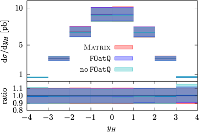
Figure 1: Comparison between fixed-order predictions from Matrix against the two MiNNLO_PS results (at “Les Houches” level) obtained using the original formulation of the method (labelled as no FOatQ) and the new one presented in this work (labelled as FOatQ). In the left pane we show the rapidity distribution of the dilepton system in Drell-Yan production, whereas in the right pane we show the Higgs boson rapidity. The ratios with respect to the Matrix results are also shown in the lower panel.

As a further validation, in figure 1 we compare the rapidity distribution of the color singlet for Drell-Yan and Higgs boson production. We show the distributions obtained with the original formulation, where the finite terms are evaluated at $\mu=p_{\mathchoice{\displaystyle}{\scriptstyle}{\scriptscriptstyle}{\scriptscriptstyle}\rm T}$ (labelled as no FOatQ), and the new one, where such terms are evaluated at $\mu=Q$, with $Q$ the invariant mass of the color singlet (labelled as FOatQ). The MiNNLO_PS results shown in the figure are obtained after generating the Powheg hardest emission, i.e. at the “Les Houches” level. In the plots we also show the NNLO results from Matrix, obtained setting $\mu=Q$. For this comparison only, we use the same PDF sets as those used in ref. Monni:2020nks . In the lower inserts of the figure we plot the ratio of the displayed distributions with respect to the Matrix result.

The curves show a very good agreement between the NNLO and the MiNNLO_PS results obtained with either formulations, both for the central scale and the uncertainty band. In particular, since the Drell-Yan process features a very small perturbative uncertainty band, the remarkable agreement between the NNLO and FOatQ curves displayed in the left pane of figure 1 is a robust validation of the new formulation of the MiNNLO_PS method.

3.3 Diphoton production: comparison with Matrix

In this section we validate the differential cross section of eq. (2.4) against the fixed-order NNLO one implemented within the public version of the Matrix code. We expect the two results to agree up to terms beyond the NNLO accuracy. The Matrix results have been obtained setting the slicing parameter $r_{\mathchoice{\displaystyle}{\scriptstyle}{\scriptscriptstyle}{\scriptscriptstyle}\rm cut}=0.0005$ and for a central scale choice $\mu_{\mathchoice{\displaystyle}{\scriptstyle}{\scriptscriptstyle}{\scriptscriptstyle}\rm R}=\mu_{\mathchoice{\displaystyle}{\scriptstyle}{\scriptscriptstyle}{\scriptscriptstyle}\rm F}=Q$. Using the isolation criteria and the fiducial cuts reported in section 3.1, the total cross section computed by Matrix and MiNNLO_PS are in agreement within the statistical errors, and they read respectively

$$\sigma_{\rm\mathchoice{\displaystyle}{\scriptstyle}{\scriptscriptstyle}{\scriptscriptstyle}tot}^{\rm\mathchoice{\displaystyle}{\scriptstyle}{\scriptscriptstyle}{\scriptscriptstyle}Matrix}=155.7\pm 1.0\leavevmode\nobreak\ {\rm pb}\,,\qquad\qquad\sigma_{\rm\mathchoice{\displaystyle}{\scriptstyle}{\scriptscriptstyle}{\scriptscriptstyle}tot}^{\rm\mathchoice{\displaystyle}{\scriptstyle}{\scriptscriptstyle}{\scriptscriptstyle}MiNNLO}=154.9\pm 0.2\leavevmode\nobreak\ {\rm pb}\,.$$ (45)

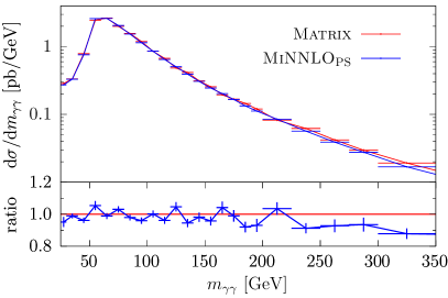
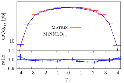
Figure 2: Comparison between fixed-order results from Matrix and MiNNLO_PS for the diphoton invariant mass and rapidity, for the default central value of the renormalization and factorization scales. The statistical errors are also shown.

In figure 2 we plot the distributions for the invariant mass and rapidity of the diphoton system computed with Matrix and MiNNLO_PS, in the top panes, and the ratio of the two curves in the lower ones. The figure shows a reasonably good agreement between the two curves within the statistical errors. We ascribe the mild difference in the high invariant-mass region to effects beyond the nominal accuracy of our result, which can differ from the purely fixed-order Matrix one by higher-order effects, present in eq. (2.4). We have explicitly verified that, by applying a transverse momentum cut on the diphoton system, the same trend is also present when we compare the exact fixed-order NLO result for $\gamma\gamma j$ production against the MiNNLO_PS one: when we move away from the region of small transverse momentum of the diphoton system that is affected by large logarithms, we still observe a mild difference between the central values of the two distributions, but still within the scale-variation bands.

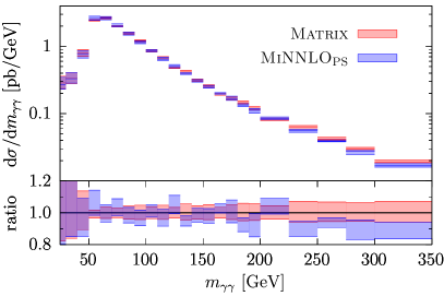
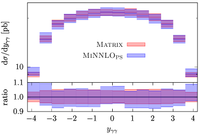
Figure 3: Comparison between fixed-order results from Matrix and MiNNLO_PS for the diphoton invariant mass and rapidity, as in figure 2. Uncertainty bands from scale variations are also shown.

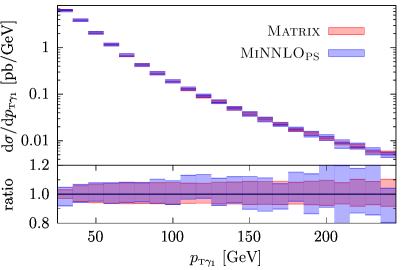
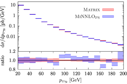
Figure 4: Comparison between fixed-order results from Matrix and MiNNLO_PS for the transverse momentum of the hardest and next-to-hardest photon. Uncertainty bands from scale variations are also shown.

The theoretical uncertainties on the Matrix and MiNNLO_PS total cross sections, estimated through a seven-point scale variation obtained by multiplying and dividing the central renormalization and factorization scales by a factor of 2, are given by

$$\sigma_{\rm\mathchoice{\displaystyle}{\scriptstyle}{\scriptscriptstyle}{\scriptscriptstyle}tot}^{\rm\mathchoice{\displaystyle}{\scriptstyle}{\scriptscriptstyle}{\scriptscriptstyle}{\sc\small{Matrix}}}=155.7\,^{+5\%}_{-4\%}\leavevmode\nobreak\ {\rm pb}\qquad\qquad\sigma_{\rm\mathchoice{\displaystyle}{\scriptstyle}{\scriptscriptstyle}{\scriptscriptstyle}tot}^{\rm\mathchoice{\displaystyle}{\scriptstyle}{\scriptscriptstyle}{\scriptscriptstyle}MiNNLO}=154.9\,^{+6\%}_{-5\%}\leavevmode\nobreak\ {\rm pb}\,,$$ (46)

and are in good agreement. In figures 3 and 4 we compare the scale variation bands obtained from the two codes for the invariant mass and rapidity distributions of the diphoton system and the transverse momentum of the hardest and next-to-hardest photon. We find an overall good agreement among the different curves, and compatible size for the scale-variation bands.

4 Phenomenological results

After validating the implementation of the MiNNLO_PS differential cross section for diphoton production given in eq. (2.4), in this section we present some distributions of physical interest obtained from the generated events, before and after passing them through a parton shower. We have generated about 16 million events without any generation cut, except for a minimum invariant mass of the diphoton system of 10 GeV. As stressed previously, except for this last constraint on the invariant mass, no other cuts have been imposed, so that these events can be used to make predictions with arbitrary fiducial cuts.

4.1 Results at partonic level

In this section we compare the Matrix results against those obtained after generating the Powheg hardest emission of eq. (35), often denoted as “Les Houches events” (LHE), and labelled in the figures as “MiNNLO_PS (LHE)”.

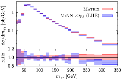
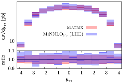
Figure 5: Comparison between the distributions obtained from the fixed-order calculation from Matrix and the results after the generation of the hardest emission, for the diphoton invariant mass and rapidity.

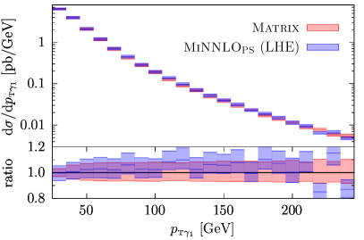
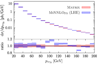
Figure 6: Comparison between the distributions obtained from the fixed-order calculation from Matrix and the results after the generation of the hardest emission, for the transverse momentum of the hardest and next-to-hardest photon.

In figure 5 we show results for the invariant mass and the rapidity of the diphoton system, whereas in figure 6 we display the transverse momentum of the hardest and next-to-hardest photon. We find good agreement between the Matrix and the MiNNLO_PS (LHE) predictions, both for the central value and for the uncertainty bands due to scale variations. Notice that, at variance with similar comparisons for other processes not involving photons (like Drell-Yan or massive diboson production), this is not trivial due to the presence of an isolation criterion in the definition of the process.

4.2 Results after parton showering

In this section we show results obtained after the completion of the parton shower performed by Pythia8 Sjostrand:2014zea ; Sjostrand:2006za . We rely on the Pythia8 interface to the Powheg Box Res, provided by the main31 configuration file, distributed with Pythia8. The results presented in this section are obtained after switching off multi-parton interactions, QED radiation and hadronization effects, using the Monash tune Skands:2014pea . We set the Pythia8 parameter POWHEG:pThard to 2 (i.e. we use the prescription introduced in section 4 of ref. Nason:2013uba ), and the SpaceShower:dipoleRecoil to 1.

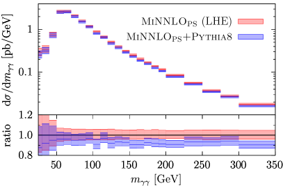
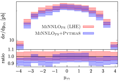
Figure 7: Comparison between the distributions obtained from the Powheg events before and after the Pythia8 parton shower for the diphoton virtuality and rapidity.

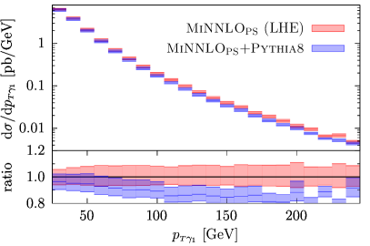
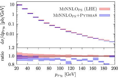
Figure 8: Comparison between the distributions obtained from the Powheg events before and after the Pythia8 parton shower for the transverse momentum of the hardest and next-to-hardest photon.

In figures 7 and 8, we present the same distributions of the previous sections, but after the Pythia8 shower. We observe a reduction of around 5–10% of the differential cross sections, compared to the MiNNLO_PS (LHE), with the largest values in the region of high transverse momenta of the two photons. We ascribe this behaviour to the fact that, with the increased multiplicity of the partonic/hadronic activity due to the Pythia8 shower, the photons in the showered events are less likely to satisfy the isolation criteria, giving a smaller cross section. We observed such pattern also for similar distributions computed with a completely independent code for diphoton production, built with the standard Powheg NLO+PS formalism, reassuring us that the above interpretation is correct, and that this behaviour is not due to some MiNNLO_PS features. We leave further investigation on this aspect for future studies.

4.3 Comparison with ATLAS results

In this section we compare our results with those presented by the ATLAS Collaboration in ref. ATLAS:2021mbt obtained at 13 TeV. In order to make a fair comparison with the experimental data, we have added to the MiNNLO_PS diphoton contribution, presented in this paper, the leading-order contribution coming from the gluon-induced production of a photon pair through a closed quark loop (denoted by $gg\rightarrow\gamma\gamma$ in the following), which is of the same order of the NNLO corrections and is further enhanced by the particularly sizable gluon luminosity. As we consider this contribution only at leading order, we simulate it at LO+PS accuracy, setting the renormalization and factorization scales, and the upper limit for the transverse momentum of the subsequent shower evolution, equal to the invariant mass of the diphoton system. The analytic amplitudes for this process have been taken from ref. Bern:2002jx and implemented in the POWHEG ​BOX ​RES framework, neglecting the top-quark loop contribution Dicus:1987fk . This contribution amounts for at most a few percent in certain regions of the kinematic distributions we are plotting. Its inclusion would improve the agreement with data.

The analysis of our events is performed using Rivet Bierlich:2019rhm , with the same Pythia8 settings as those in the previous section. The fiducial volume is defined by the following requirements

$${p_{{\mathchoice{\displaystyle}{\scriptstyle}{\scriptscriptstyle}{\scriptscriptstyle}\rm T}\gamma_{1}}}>40\leavevmode\nobreak\ {\rm GeV},\qquad{p_{{\mathchoice{\displaystyle}{\scriptstyle}{\scriptscriptstyle}{\scriptscriptstyle}\rm T}\gamma_{2}}}>30\leavevmode\nobreak\ {\rm GeV},\qquad\Delta R_{\gamma\gamma}>0.4\,,$$

$$|y_{\gamma}|<1.37\,,\qquad 1.52<|y_{\gamma}|<2.37.$$ (47)

We do not report here the exact photon-isolation criteria which are described in detail in section 4.1 of ref. ATLAS:2021mbt .

In figures 9 and 10

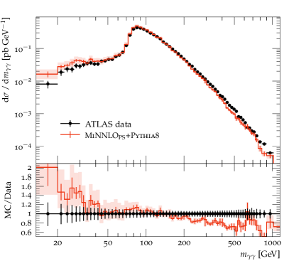
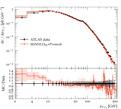
Figure 9: Comparison between the ATLAS data and the distributions obtained with MiNNLO_PS+Pythia8, for the diphoton invariant mass and its transverse momentum. Scale-variation bands are also shown, together with the statistical errors of the central value.

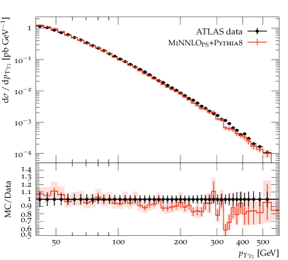
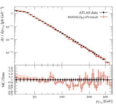
Figure 10: Comparison between the ATLAS data and the distributions obtained with MiNNLO_PS+Pythia8, for the transverse momentum of the leading and subleading photon. Scale-variation bands are also shown, together with the statistical errors of the central value.

we show the invariant mass and the transverse momentum of the diphoton system, and the transverse momentum of the leading and subleading photon, respectively. Overall we find a reasonably good agreement between data and theoretical predictions.

For the invariant mass distribution $m_{\gamma\gamma}$ we observe a good agreement in the bulk of the cross section. Given the cuts of eq. (47), the region where $m_{\gamma\gamma}<80$ GeV is populated only by $\gamma\gamma$ + jet(s) events, therefore our results are only NLO+PS accurate, as confirmed also by the wider uncertainty bands. For $m_{\gamma\gamma}\lesssim 40$ GeV, MiNNLO_PS results overshoot ATLAS data by an amount compatible with what has been observed, for other predictions of similar accuracy, in ref. ATLAS:2021mbt . This is particularly true for the first bin. The fact that this region is characterized by a large NLO $K$-factor Catani:2018krb hints at the possibility that the inclusion of higher-order corrections will improve the agreement with data. At large $m_{\gamma\gamma}$ values we observe differences up to about 15%. Such differences might be due to the absence of higher-order effects. Top-quark mass effects above the threshold $m_{\gamma\gamma}\simeq 2m_{t}$, that we are neglecting in the quark-induced 2-loop amplitudes as well as in the $gg\rightarrow\gamma\gamma$ channel, can also induce differences at a few percent level.

As far as the transverse-momentum spectrum of the diphoton pair is concerned, our predictions are compatible with experimental data across most of the $p_{{\mathchoice{\displaystyle}{\scriptstyle}{\scriptscriptstyle}{\scriptscriptstyle}\rm T}\gamma\gamma}$ spectrum, within the estimated theoretical uncertainties. Due to the all-order treatment of soft and collinear radiation encoded in the MiNNLO_PS Sudakov form factor and in the subsequent matching to Pythia, the region of small $p_{{\mathchoice{\displaystyle}{\scriptstyle}{\scriptscriptstyle}{\scriptscriptstyle}\rm T}\gamma\gamma}$ is in a fair agreement with the data, within the statistical error and the scale-variation band. For large values of $p_{{\mathchoice{\displaystyle}{\scriptstyle}{\scriptscriptstyle}{\scriptscriptstyle}\rm T}\gamma\gamma}$, data and theoretical predictions agree well in shape but display a flat offset of about 10%.

The comparison of our results against ATLAS data for the $p_{\mathchoice{\displaystyle}{\scriptstyle}{\scriptscriptstyle}{\scriptscriptstyle}\rm T}$ spectrum of the leading and subleading photon is shown in figure 10. Data and theoretical predictions agree quite well over the full range of the transverse momentum.

We would also like to point out that the choices for the central value of the renormalization and factorization scales, in a fixed-order computation, can have a sizable impact on the theory predictions at large invariant mass and transverse momentum of the diphoton system, as discussed in detail e.g. in ref. Gehrmann:2020oec . The size of these effects are a consequence of a slowly convergent perturbative series. Assessing this type of effects by exploring different scale choices in our MiNNLO_PS simulation goes beyond the scope of this paper, although this is a-priori possible, both for the handling of the large-$p_{\mathchoice{\displaystyle}{\scriptstyle}{\scriptscriptstyle}{\scriptscriptstyle}\rm T}$ limit of the singular component (first term of eq. (2.4)), as discussed for instance in ref. Mazzitelli:2021mmm , as well as for the scales used in the non-singular contribution (last term in the same equation).

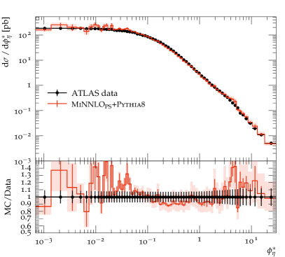
Figure 11: Comparison between the ATLAS data and the distributions obtained with MiNNLO_PS+Pythia8, for the azimuthal separation of the two photons $\Delta\phi_{\gamma\gamma}$ and for $\phi_{\eta}^{*}$, as defined in eq. (48). Scale-variation bands are also shown, together with the statistical errors of the central value.

In figure 11 we show the differential cross section as a function of two angular observables: the azimuthal separation $\Delta\phi_{\gamma\gamma}$ of the two photons and $\phi_{\eta}^{*}$, defined as

$$\phi_{\eta}^{*}=\tan\frac{\pi-\Delta\phi_{\gamma\gamma}}{2}\,\sin\theta_{\eta}^{*}=\tan\frac{\pi-\Delta\phi_{\gamma\gamma}}{2}\,\sqrt{1-\left(\tanh\frac{\Delta y_{\gamma\gamma}}{2}\right)^{2}},$$ (48)

where $\Delta y_{\gamma\gamma}$ is the azimuthal angular separation of the two photons. Such variable, first introduced for Drell-Yan processes in ref. Banfi:2010cf , is known to be sensitive to the same dynamics governing the ${p_{\mathchoice{\displaystyle}{\scriptstyle}{\scriptscriptstyle}{\scriptscriptstyle}\rm T}}_{\gamma\gamma}$ spectrum, but it allows for a better resolution at small values of ${p_{\mathchoice{\displaystyle}{\scriptstyle}{\scriptscriptstyle}{\scriptscriptstyle}\rm T}}_{\gamma\gamma}$. The agreement between data and the theoretical predictions is rather good on the whole range within the statistical and scale-variation bands. We stress that, for $\Delta\phi_{\gamma\gamma}\rightarrow\pi$, the NNLO fixed-order results for the above distributions are divergent, while we get a finite distributions due to the MiNNLO Sudakov form factor.

5 Conclusions

In this paper we have presented the implementation of a new MiNNLO_PS event generator accurate at NNLO in QCD for the production of a photon pair in hadronic collisions, within the Powheg Box Res framework. This implementation is based on the MiNNLO_PS formalism presented in refs. Monni:2019whf ; Monni:2020nks , that we have modified in order to deal with the new features needed to describe a process with photons at the Born level. We have devised and implemented a general method to deal with the presence of QED singularities at the Born level within the Powheg Box Res, and we have presented a new mapping from $\gamma\gamma j$ to the $\gamma\gamma$. The combined use of the new mapping and of the method to deal with the QED divergences allowed us to simulate diphoton production at NNLO+PS accuracy without introducing any generation or technical cut. Our generator produces weighted events that cover the entire phase space, thereby allowing the generated sample to be used with arbitrary fiducial cuts.

Furthermore, we have introduced a few modifications to the MiNNLO_PS formalism, that do not change the formal accuracy of the method and reduce the numerical impact of higher-order terms, thus leading to better agreement with fixed-order computations. We have also verified that the new formulation of MiNNLO_PS, when applied to the original MiNNLO_PS implementations with massive bosons, gives results fully compatible with the original one.

Finally, we have presented some distributions of physical interest obtained from the generated events both before and after passing them through the parton shower, and compared them with the ATLAS results at 13 TeV. Using the standard settings of Pythia8 when interfacing it with the Powheg Box Res, we observe a reduction of about 5–10% of the inclusive differential cross sections compared to the NNLO fixed-order ones. We ascribe this effect to the increased multiplicity of the partonic/hadronic activity coming from the shower causing the photons to less likely satisfy the isolation criteria. Further investigation of the matching procedure between Powheg Box Res+MiNNLO_PS and Pythia8 is left for future studies.

Appendix A The $\boldsymbol{\Phi_{\mathchoice{\displaystyle}{\scriptstyle}{\scriptscriptstyle}{\scriptscriptstyle}\gamma\gamma j}}\rightarrow\boldsymbol{\Phi_{\mathchoice{\displaystyle}{\scriptstyle}{\scriptscriptstyle}{\scriptscriptstyle}\gamma\gamma}}$ phase space projection

In section 2.3 it was shown that one needs a mapping from the $\Phi_{\mathchoice{\displaystyle}{\scriptstyle}{\scriptscriptstyle}{\scriptscriptstyle}\gamma\gamma j}$ phase space to the $\Phi_{\mathchoice{\displaystyle}{\scriptstyle}{\scriptscriptstyle}{\scriptscriptstyle}\gamma\gamma}$ one, and this mapping should be smooth when $p_{\mathchoice{\displaystyle}{\scriptstyle}{\scriptscriptstyle}{\scriptscriptstyle}\rm T}\rightarrow 0$, i.e. when the final-state jet is soft or collinear with the incoming beams.

This projection plays a more important role for the process under study than in previous processes dealt within the MiNNLO_PS procedure. In fact, for diphoton production, we would like to avoid that the kinematics of a $\gamma\gamma j$ event that is away from any collinear divergence is projected on a kinematics for $\gamma\gamma$ production, where the photons are quasi-collinear with the incoming beams, which would give divergent contributions for the $pp\rightarrow\gamma\gamma$ matrix elements needed in the MiNNLO_PS $D$ terms (see section 2.4). This projection is determined by the requirements that it preserves the mass and rapidity of the color singlet, and the direction of one of the photons in the laboratory frame.

As far as the MiNNLO_PS formulae are concerned, we just need to define a $\Phi_{\mathchoice{\displaystyle}{\scriptstyle}{\scriptscriptstyle}{\scriptscriptstyle}\gamma\gamma j}\rightarrow\Phi_{\mathchoice{\displaystyle}{\scriptstyle}{\scriptscriptstyle}{\scriptscriptstyle}\gamma\gamma}$ mapping that projects a $\Phi_{\mathchoice{\displaystyle}{\scriptstyle}{\scriptscriptstyle}{\scriptscriptstyle}\gamma\gamma j}$ phase-space point to a $\Phi_{\mathchoice{\displaystyle}{\scriptstyle}{\scriptscriptstyle}{\scriptscriptstyle}\gamma\gamma}$ one. In addition to this, we also provide the inverse mapping, that will be used to compute the Jacobian of the transformation in section A.3.

A.1 The $\boldsymbol{\Phi_{\mathchoice{\displaystyle}{\scriptstyle}{\scriptscriptstyle}{\scriptscriptstyle}\gamma\gamma j}}$ kinematics

In the partonic center-of-mass frame, momentum conservation reads

$$p_{\mathchoice{\displaystyle}{\scriptstyle}{\scriptscriptstyle}{\scriptscriptstyle}\oplus}+p_{\mathchoice{\displaystyle}{\scriptstyle}{\scriptscriptstyle}{\scriptscriptstyle}\ominus}=p_{\gamma_{1}}+p_{\gamma_{2}}+p_{\mathchoice{\displaystyle}{\scriptstyle}{\scriptscriptstyle}{\scriptscriptstyle}j}\,,$$ (49)

where

$$p_{\mathchoice{\displaystyle}{\scriptstyle}{\scriptscriptstyle}{\scriptscriptstyle}\oplus}=\frac{\sqrt{s}}{2}(1,0,0,1)\,,\qquad\qquad p_{\mathchoice{\displaystyle}{\scriptstyle}{\scriptscriptstyle}{\scriptscriptstyle}\ominus}=\frac{\sqrt{s}}{2}(1,0,0,-1)\,,$$ (50)

and $s$ is the squared center-of-mass energy. In this section, at difference with the rest of the paper, we denote with $p_{\gamma_{1}}$ and $p_{\gamma_{2}}$ the momenta of the two photons, irrespectively of which one is the hardest or the softest. Using the standard FKS Frixione:1995ms radiation variables $\xi$, $y$ and $\phi_{\mathchoice{\displaystyle}{\scriptstyle}{\scriptscriptstyle}{\scriptscriptstyle}j}$, we write the jet momentum as

$$p_{\mathchoice{\displaystyle}{\scriptstyle}{\scriptscriptstyle}{\scriptscriptstyle}j}=\frac{\sqrt{s}}{2}\,\xi\left(1,\,\sin\theta_{\mathchoice{\displaystyle}{\scriptstyle}{\scriptscriptstyle}{\scriptscriptstyle}j}\sin\phi_{\mathchoice{\displaystyle}{\scriptstyle}{\scriptscriptstyle}{\scriptscriptstyle}j},\,\sin\theta_{\mathchoice{\displaystyle}{\scriptstyle}{\scriptscriptstyle}{\scriptscriptstyle}j}\cos\phi_{\mathchoice{\displaystyle}{\scriptstyle}{\scriptscriptstyle}{\scriptscriptstyle}j},\,\cos\theta_{\mathchoice{\displaystyle}{\scriptstyle}{\scriptscriptstyle}{\scriptscriptstyle}j}\right),$$ (51)

where $\cos\theta_{\mathchoice{\displaystyle}{\scriptstyle}{\scriptscriptstyle}{\scriptscriptstyle}j}=y$. Using eq. (49), the momentum of the diphoton system is then given by

$$p_{\gamma\gamma}=\frac{\sqrt{s}}{2}\,\left(2-\xi,\,-\xi\sqrt{1-y^{2}}\sin\phi_{\mathchoice{\displaystyle}{\scriptstyle}{\scriptscriptstyle}{\scriptscriptstyle}j},\,-\xi\sqrt{1-y^{2}}\cos\phi_{\mathchoice{\displaystyle}{\scriptstyle}{\scriptscriptstyle}{\scriptscriptstyle}j},\,-\xi y\right),$$ (52)

that has invariant mass and rapidity given by

$$m_{\gamma\gamma}=\sqrt{s\left(1-\xi\right)}\,,\qquad\qquad y_{\gamma\gamma}^{\mathchoice{\displaystyle}{\scriptstyle}{\scriptscriptstyle}{\scriptscriptstyle}\rm CM}=\frac{1}{2}\log\!\left(\frac{2-\xi-\xi y}{2-\xi+\xi y}\right)\,.$$ (53)

A.2 From $\boldsymbol{\Phi_{\mathchoice{\displaystyle}{\scriptstyle}{\scriptscriptstyle}{\scriptscriptstyle}\gamma\gamma}}$ to $\boldsymbol{\Phi_{\mathchoice{\displaystyle}{\scriptstyle}{\scriptscriptstyle}{\scriptscriptstyle}\gamma\gamma j}}$

In order to preserve the direction of one photon, we need to express the momenta of the involved particles in two frames where the diphoton system has the same rapidity. We choose to work in the center-of-mass frame of the $\gamma\gamma j$ system because, in this frame, the momentum of the final-state parton has a simple representation in terms of the FKS variables, as given in eq. (51). We parametrize the momenta of the two photons in their center-of-mass frame as

$$\left\{\begin{array}[]{l}\displaystyle\bar{p}_{\gamma_{1}}=\frac{m_{\gamma\gamma}}{2}\left(1,\,\sin\bar{\theta}\sin\bar{\varphi},\,\sin\bar{\theta}\cos\bar{\varphi},\,\cos\bar{\theta}\right),\nobreak\leavevmode\\[8.53581pt] \displaystyle\bar{p}_{\gamma_{2}}=\frac{m_{\gamma\gamma}}{2}\left(1,\,-\sin\bar{\theta}\sin\bar{\varphi},\,-\sin\bar{\theta}\cos\bar{\varphi},\,-\cos\bar{\theta}\right),\end{array}\right.$$ (54)

and we then perform a longitudinal boost with rapidity $y_{\gamma\gamma}^{\mathchoice{\displaystyle}{\scriptstyle}{\scriptscriptstyle}{\scriptscriptstyle}\rm CM}$ of eq. (53) to obtain

$$\left\{\begin{array}[]{l}\displaystyle\bar{p}^{\prime}_{\gamma_{1}}=\frac{m_{\gamma\gamma}}{2}\left(\frac{2-\xi-\xi y\cos\bar{\theta}}{r},\,\sin\bar{\theta}\sin\bar{\varphi},\,\sin\bar{\theta}\cos\bar{\varphi},\,\frac{(2-\xi)\cos\bar{\theta}-\xi y}{r}\right),\\[8.53581pt] \displaystyle\bar{p}^{\prime}_{\gamma_{2}}=\frac{m_{\gamma\gamma}}{2}\left(\frac{2-\xi+\xi y\cos\bar{\theta}}{r},\,-\sin\bar{\theta}\sin\bar{\varphi},\,-\sin\bar{\theta}\cos\bar{\varphi},\,\frac{-(2-\xi)\cos\bar{\theta}-\xi y}{r}\right),\end{array}\right.$$ (55)

where

$$r=\sqrt{(2-\xi)^{2}-\xi^{2}y^{2}}\,.$$ (56)

We now impose that the momentum $p_{\gamma_{1}}$ in the partonic center-of-mass frame of $\gamma\gamma j$ has the same direction as $\bar{p}^{\prime}_{\gamma_{1}}$. In this way, if the photon $\gamma_{1}$ of $\Phi_{\mathchoice{\displaystyle}{\scriptstyle}{\scriptscriptstyle}{\scriptscriptstyle}\gamma\gamma}$ becomes too close to the incoming beams, then also the photon $\gamma_{1}$ of $\Phi_{\mathchoice{\displaystyle}{\scriptstyle}{\scriptscriptstyle}{\scriptscriptstyle}\gamma\gamma j}$ will be close to the beams, and will be suppressed by the Born suppression factors of eq. (36). To achieve this, we change the energy of $\bar{p}^{\prime}_{\gamma_{1}}$, introducing the dimensionless parameter ${\cal E}$, such that the momentum of $\gamma_{1}$ in the center-of-mass frame kinematics of $\Phi_{\mathchoice{\displaystyle}{\scriptstyle}{\scriptscriptstyle}{\scriptscriptstyle}\gamma\gamma j}$ is given by

$$p_{\gamma_{1}}={\cal E}\,\sqrt{s}\left(\frac{2-\xi-\xi y\cos\bar{\theta}}{r},\,\sin\bar{\theta}\sin\bar{\varphi},\,\sin\bar{\theta}\cos\bar{\varphi},\,\frac{(2-\xi)\cos\bar{\theta}-\xi y}{r}\right).$$ (57)

We fix the value of ${\cal E}$ by imposing that the second photon stays massless. In fact, from the momentum conservation of eq. (49)

$$p_{\gamma_{2}} = p_{\mathchoice{\displaystyle}{\scriptstyle}{\scriptscriptstyle}{\scriptscriptstyle}\oplus}+p_{\mathchoice{\displaystyle}{\scriptstyle}{\scriptscriptstyle}{\scriptscriptstyle}\ominus}-p_{\gamma_{1}}-p_{\mathchoice{\displaystyle}{\scriptstyle}{\scriptscriptstyle}{\scriptscriptstyle}j}$$ (58)

$$= \sqrt{s}\left(1-\frac{\xi}{2}-{\cal E}\,\frac{2-\xi-\xi y\cos\bar{\theta}}{r},\,-\frac{\xi}{2}\sqrt{1-y^{2}}\sin\phi_{\mathchoice{\displaystyle}{\scriptstyle}{\scriptscriptstyle}{\scriptscriptstyle}j}-{\cal E}\sin\bar{\theta}\sin\bar{\varphi},\,\right.$$

$$\hskip 22.76219pt\left.-\frac{\xi}{2}\sqrt{1-y^{2}}\cos\phi_{\mathchoice{\displaystyle}{\scriptstyle}{\scriptscriptstyle}{\scriptscriptstyle}j}-{\cal E}\sin\bar{\theta}\cos\bar{\varphi},\,-\frac{\xi y}{2}-{\cal E}\,\frac{(2-\xi)\cos\bar{\theta}-\xi y}{r}\right),$$

and by imposing $p_{\gamma_{2}}^{2}=0$ we have

$${\cal E}=\frac{1-\xi}{r+\xi\sqrt{1-y^{2}}\sin\bar{\theta}\cos(\phi_{\mathchoice{\displaystyle}{\scriptstyle}{\scriptscriptstyle}{\scriptscriptstyle}j}-\bar{\varphi})}\,.$$ (59)

Once the momenta $p_{\mathchoice{\displaystyle}{\scriptstyle}{\scriptscriptstyle}{\scriptscriptstyle}j}$, $p_{\gamma_{1}}$ and $p_{\gamma_{2}}$, given by eqs. (51), (57) and (58) are known in their partonic center-of-mass frame, we can obtain their expression in the laboratory system by performing a longitudinal boost with the rapidity of the center-of-mass system.

A.3 The Jacobian of the mapping

In order to conclude the procedure to build $\Phi_{\mathchoice{\displaystyle}{\scriptstyle}{\scriptscriptstyle}{\scriptscriptstyle}\gamma\gamma j}$ from $\Phi_{\mathchoice{\displaystyle}{\scriptstyle}{\scriptscriptstyle}{\scriptscriptstyle}\gamma\gamma}$, we need to compute the Jacobian of the transformation we have outlined in the previous section. Following the Powheg notation Frixione:2007vw ; Alioli:2010xd , we write the infinitesimal phase space volume in terms of the Bjorken $x$ as

$$\mathrm{d}\Phi_{3}\equiv\mathrm{d}x_{\mathchoice{\displaystyle}{\scriptstyle}{\scriptscriptstyle}{\scriptscriptstyle}\oplus}\,\mathrm{d}x_{\mathchoice{\displaystyle}{\scriptstyle}{\scriptscriptstyle}{\scriptscriptstyle}\ominus}\,\mathrm{d}\Phi_{\gamma\gamma j}={\mathrm{d}\bar{x}_{\mathchoice{\displaystyle}{\scriptstyle}{\scriptscriptstyle}{\scriptscriptstyle}\oplus}\,\mathrm{d}\bar{x}_{\mathchoice{\displaystyle}{\scriptstyle}{\scriptscriptstyle}{\scriptscriptstyle}\ominus}}\,\mathrm{d}\Phi_{\mathchoice{\displaystyle}{\scriptstyle}{\scriptscriptstyle}{\scriptscriptstyle}{\rm rad}}\,\mathrm{d}\Phi_{\gamma\gamma}\,,$$ (60)

where

$$\mathrm{d}\Phi_{\mathchoice{\displaystyle}{\scriptstyle}{\scriptscriptstyle}{\scriptscriptstyle}{\rm rad}}\equiv\frac{s}{(4\pi)^{3}}\,\frac{\xi}{1-\xi}\,\mathrm{d}\xi\,\mathrm{d}y\,\mathrm{d}\phi_{\mathchoice{\displaystyle}{\scriptstyle}{\scriptscriptstyle}{\scriptscriptstyle}j}\,,$$ (61)

is written using the FKS radiation variables. We would like to express $\mathrm{d}\Phi_{\gamma\gamma}$ using the polar and azimuthal angle of one photon in the center-of-mass frame of the diphoton system, i.e. $\theta^{\prime}$ and $\varphi^{\prime}$, where it can be written as

$$\mathrm{d}\Phi_{\gamma\gamma}=\frac{1}{32\pi^{2}}\,\mathrm{d}\cos\theta^{\prime}\,\mathrm{d}\varphi^{\prime}\,,$$ (62)

in terms of the angles of our mapping, i.e. $\bar{\theta}$ and $\bar{\varphi}$, that we have used to write eqs. (57) and (58). Using the fact that $\mathrm{d}\Phi_{\gamma\gamma}$ is a Lorentz scalar, we need to compute the Jacobian $J$ that relates the change of variables

$$\mathrm{d}\Phi_{\gamma\gamma}=\frac{J}{32\pi^{2}}\,\mathrm{d}\cos\bar{\theta}\,\mathrm{d}\bar{\varphi}\,.$$ (63)

In order to do this, we find the sequence of boosts from the partonic center-of-mass frame of $\gamma\gamma j$ to the center-of-mass frame of the diphoton system. We first perform a longitudinal boost of the momenta $p_{\gamma_{1}}$ and $p_{\gamma_{2}}$ of eqs. (57) and (58) to the frame where the diphoton system has zero rapidity. The longitudinal rapidity of the boost is given by eq. (53) and we obtain

$$\displaystyle p_{\gamma_{1}}^{\mathchoice{\displaystyle}{\scriptstyle}{\scriptscriptstyle}{\scriptscriptstyle}\rm L} = {\cal E}\,\sqrt{s}\left(1,\,\sin\bar{\theta}\sin\bar{\varphi},\,\sin\bar{\theta}\cos\bar{\varphi},\,\cos\bar{\theta}\right),$$

$$\displaystyle p_{\gamma_{2}}^{\mathchoice{\displaystyle}{\scriptstyle}{\scriptscriptstyle}{\scriptscriptstyle}\rm L} = \sqrt{s}\left(\frac{r}{2}-{\cal E},\,-\frac{\xi}{2}\sqrt{1-y^{2}}\sin\phi_{\mathchoice{\displaystyle}{\scriptstyle}{\scriptscriptstyle}{\scriptscriptstyle}j}-{\cal E}\sin\bar{\theta}\sin\bar{\varphi},\,\right.$$ (64)

$$\mbox{}\hskip 56.9055pt\left.-\frac{\xi}{2}\sqrt{1-y^{2}}\cos\phi_{\mathchoice{\displaystyle}{\scriptstyle}{\scriptscriptstyle}{\scriptscriptstyle}j}-{\cal E}\sin\bar{\theta}\cos\bar{\varphi},\,-{\cal E}\cos\bar{\theta}\right).$$

Then we perform a transverse boost to the diphoton rest system with transverse velocity

$$\boldsymbol{v_{\mathchoice{\displaystyle}{\scriptstyle}{\scriptscriptstyle}{\scriptscriptstyle}\rm T}}=-\frac{\xi\sqrt{1-y^{2}}}{r}\left(\sin\phi_{\mathchoice{\displaystyle}{\scriptstyle}{\scriptscriptstyle}{\scriptscriptstyle}j},\,\cos\phi_{\mathchoice{\displaystyle}{\scriptstyle}{\scriptscriptstyle}{\scriptscriptstyle}j},\,0\right),$$ (65)

and we get

$$p_{\gamma_{1}}^{\mathchoice{\displaystyle}{\scriptstyle}{\scriptscriptstyle}{\scriptscriptstyle}\rm T}=\frac{m_{\gamma\gamma}}{2}\left(1,\boldsymbol{p_{\gamma_{1}}^{\mathchoice{\displaystyle}{\scriptstyle}{\scriptscriptstyle}{\scriptscriptstyle}\rm T}}\right),\qquad\qquad p_{\gamma_{2}}^{\mathchoice{\displaystyle}{\scriptstyle}{\scriptscriptstyle}{\scriptscriptstyle}\rm T}=\frac{m_{\gamma\gamma}}{2}\left(1,-\boldsymbol{p_{\gamma_{1}}^{\mathchoice{\displaystyle}{\scriptstyle}{\scriptscriptstyle}{\scriptscriptstyle}\rm T}}\right),$$ (66)

where

$$\boldsymbol{p_{\gamma_{1}}^{\mathchoice{\displaystyle}{\scriptstyle}{\scriptscriptstyle}{\scriptscriptstyle}\rm T}} = \frac{1}{r+\xi\sqrt{1-y^{2}}\sin\bar{\theta}\cos(\phi_{\mathchoice{\displaystyle}{\scriptstyle}{\scriptscriptstyle}{\scriptscriptstyle}j}-\bar{\varphi})}$$ (67)

$$\times\Bigg{(}\sin\phi_{\mathchoice{\displaystyle}{\scriptstyle}{\scriptscriptstyle}{\scriptscriptstyle}j}\left(r\sin\bar{\theta}\cos(\bar{\varphi}-\phi_{\mathchoice{\displaystyle}{\scriptstyle}{\scriptscriptstyle}{\scriptscriptstyle}j})+\xi\sqrt{1-y^{2}}\right)+2\sqrt{1-\xi}\cos\phi_{\mathchoice{\displaystyle}{\scriptstyle}{\scriptscriptstyle}{\scriptscriptstyle}j}\sin\bar{\theta}\sin(\bar{\varphi}-\phi_{\mathchoice{\displaystyle}{\scriptstyle}{\scriptscriptstyle}{\scriptscriptstyle}j})\,,$$

$$\hskip 17.07164pt\cos\phi_{\mathchoice{\displaystyle}{\scriptstyle}{\scriptscriptstyle}{\scriptscriptstyle}j}\left(r\sin\bar{\theta}\cos(\bar{\varphi}-\phi_{\mathchoice{\displaystyle}{\scriptstyle}{\scriptscriptstyle}{\scriptscriptstyle}j})+\xi\sqrt{1-y^{2}}\right)-2\sqrt{1-\xi}\sin\phi_{\mathchoice{\displaystyle}{\scriptstyle}{\scriptscriptstyle}{\scriptscriptstyle}j}\sin\bar{\theta}\sin(\bar{\varphi}-\phi_{\mathchoice{\displaystyle}{\scriptstyle}{\scriptscriptstyle}{\scriptscriptstyle}j})\,,$$

$$\hskip 17.07164pt2\sqrt{1-\xi}\cos\bar{\theta}\Bigg{)}.$$

In the diphoton rest system, $\boldsymbol{p_{\gamma_{1}}^{\mathchoice{\displaystyle}{\scriptstyle}{\scriptscriptstyle}{\scriptscriptstyle}\rm T}}$, written as a function of $\theta^{\prime}$ and $\varphi^{\prime}$, has components

$$\boldsymbol{p_{\gamma_{1}}^{\mathchoice{\displaystyle}{\scriptstyle}{\scriptscriptstyle}{\scriptscriptstyle}\rm T}}\equiv\left(\sin\theta^{\prime}\sin\varphi^{\prime},\,\sin\theta^{\prime}\cos\varphi^{\prime},\,\cos\theta^{\prime}\right).$$ (68)

By comparing eqs. (67) and (68), we can write

$$\cos\theta^{\prime} = \frac{2\sqrt{1-\xi}\cos\bar{\theta}}{r+\xi\sqrt{1-y^{2}}\sin\bar{\theta}\cos(\phi_{\mathchoice{\displaystyle}{\scriptstyle}{\scriptscriptstyle}{\scriptscriptstyle}j}-\bar{\varphi})}$$ (69)

$$\tan\varphi^{\prime} = \frac{\sin\phi_{\mathchoice{\displaystyle}{\scriptstyle}{\scriptscriptstyle}{\scriptscriptstyle}j}\left(r\sin\bar{\theta}\cos(\bar{\varphi}-\phi_{\mathchoice{\displaystyle}{\scriptstyle}{\scriptscriptstyle}{\scriptscriptstyle}j})+\xi\sqrt{1-y^{2}}\right)+2\sqrt{1-\xi}\cos\phi_{\mathchoice{\displaystyle}{\scriptstyle}{\scriptscriptstyle}{\scriptscriptstyle}j}\sin\bar{\theta}\sin(\bar{\varphi}-\phi_{\mathchoice{\displaystyle}{\scriptstyle}{\scriptscriptstyle}{\scriptscriptstyle}j})}{\cos\phi_{\mathchoice{\displaystyle}{\scriptstyle}{\scriptscriptstyle}{\scriptscriptstyle}j}\left(r\sin\bar{\theta}\cos(\bar{\varphi}-\phi_{\mathchoice{\displaystyle}{\scriptstyle}{\scriptscriptstyle}{\scriptscriptstyle}j})+\xi\sqrt{1-y^{2}}\right)-2\sqrt{1-\xi}\sin\phi_{\mathchoice{\displaystyle}{\scriptstyle}{\scriptscriptstyle}{\scriptscriptstyle}j}\sin\bar{\theta}\sin(\bar{\varphi}-\phi_{\mathchoice{\displaystyle}{\scriptstyle}{\scriptscriptstyle}{\scriptscriptstyle}j})}$$

and from these expressions, we can compute the Jacobian $J$

$$J=\frac{\partial{\left(\cos\theta^{\prime},\varphi^{\prime}\right)}}{\partial\left(\cos\bar{\theta},\bar{\varphi}\right)}=\frac{4(1-\xi)}{\left(r+\xi\sqrt{1-y^{2}}\sin\bar{\theta}\cos(\bar{\varphi}-\phi_{\mathchoice{\displaystyle}{\scriptstyle}{\scriptscriptstyle}{\scriptscriptstyle}j})\right)^{2}}\,.$$ (71)

This completes the calculation of the direct and inverse mapping $\Phi_{\mathchoice{\displaystyle}{\scriptstyle}{\scriptscriptstyle}{\scriptscriptstyle}\gamma\gamma j}\leftrightarrow\Phi_{\mathchoice{\displaystyle}{\scriptstyle}{\scriptscriptstyle}{\scriptscriptstyle}\gamma\gamma}$ and the construction of the three-body phase space, from one side, and of its inverse mapping, on the other.

Appendix B MiNNLO_PS formulae

In this section, we provide the explicit expressions for the ingredients needed in the MiNNLO_PS formulae, focussing in particular on their renormalization and factorization scale dependence. We use the same notation as ref. Monni:2019whf , and we refer the interested reader to this paper for further details. For ease of notation, we drop all the dependences on the kinematic variables, and we retain only that on the scales, which we assume to be equal, $\mu_{\mathrm{R}}=\mu_{\mathrm{F}}=\mu$. In section 2.4, a physical quantity $G$ computed at scale $\mu$ was indicated with $\left[G\!\left(\Phi_{\mathchoice{\displaystyle}{\scriptstyle}{\scriptscriptstyle}{\scriptscriptstyle}\gamma\gamma},p_{\mathchoice{\displaystyle}{\scriptstyle}{\scriptscriptstyle}{\scriptscriptstyle}\rm T}\right)\right]_{\mu}$. In the compact notation of this section, is is now simply written as $G(\mu)$.

Using this notation, from the definition of $D$ in eq. (25) and of its expansion in eq. (28), we have

$$\left[D\!\left(p_{\mathchoice{\displaystyle}{\scriptstyle}{\scriptscriptstyle}{\scriptscriptstyle}\rm T}\right)\right]^{(1)} = \left[\frac{d{{\cal L}}\!\left(p_{\mathchoice{\displaystyle}{\scriptstyle}{\scriptscriptstyle}{\scriptscriptstyle}\rm T}\right)}{dp_{\mathchoice{\displaystyle}{\scriptstyle}{\scriptscriptstyle}{\scriptscriptstyle}\rm T}}\right]^{\!(1)}-\left[{\cal L}\!\left(p_{\mathchoice{\displaystyle}{\scriptstyle}{\scriptscriptstyle}{\scriptscriptstyle}\rm T}\right)\right]^{(0)}\left[\frac{d\tilde{S}\!\left(p_{\mathchoice{\displaystyle}{\scriptstyle}{\scriptscriptstyle}{\scriptscriptstyle}\rm T}\right)}{dp_{\mathchoice{\displaystyle}{\scriptstyle}{\scriptscriptstyle}{\scriptscriptstyle}\rm T}}\right]^{\!(1)}$$ (72)

$$\left[D\!\left(p_{\mathchoice{\displaystyle}{\scriptstyle}{\scriptscriptstyle}{\scriptscriptstyle}\rm T}\right)\right]^{(2)} = \left[\frac{d{{\cal L}}\!\left(p_{\mathchoice{\displaystyle}{\scriptstyle}{\scriptscriptstyle}{\scriptscriptstyle}\rm T}\right)}{dp_{\mathchoice{\displaystyle}{\scriptstyle}{\scriptscriptstyle}{\scriptscriptstyle}\rm T}}\right]^{\!(2)}-\left[{\cal L}\!\left(p_{\mathchoice{\displaystyle}{\scriptstyle}{\scriptscriptstyle}{\scriptscriptstyle}\rm T}\right)\right]^{(0)}\left[\frac{d\tilde{S}\!\left(p_{\mathchoice{\displaystyle}{\scriptstyle}{\scriptscriptstyle}{\scriptscriptstyle}\rm T}\right)}{dp_{\mathchoice{\displaystyle}{\scriptstyle}{\scriptscriptstyle}{\scriptscriptstyle}\rm T}}\right]^{\!(2)}-\left[{\cal L}\!\left(p_{\mathchoice{\displaystyle}{\scriptstyle}{\scriptscriptstyle}{\scriptscriptstyle}\rm T}\right)\right]^{(1)}\left[\frac{d\tilde{S}\!\left(p_{\mathchoice{\displaystyle}{\scriptstyle}{\scriptscriptstyle}{\scriptscriptstyle}\rm T}\right)}{dp_{\mathchoice{\displaystyle}{\scriptstyle}{\scriptscriptstyle}{\scriptscriptstyle}\rm T}}\right]^{\!(1)}.$$ (73)

The explicit expression for the luminosity ${\cal L}$, evaluated at scales $p_{\mathchoice{\displaystyle}{\scriptstyle}{\scriptscriptstyle}{\scriptscriptstyle}\rm T}$, is

$${\cal L}\!\left(p_{\mathchoice{\displaystyle}{\scriptstyle}{\scriptscriptstyle}{\scriptscriptstyle}\rm T}\right)=\sum_{cd}\left|M_{cd\rightarrow\gamma\gamma}\right|^{2}\tilde{H}_{cd\rightarrow\gamma\gamma}\sum_{ij}\left(\tilde{C}_{ci}\otimes f_{i}^{[a]}\right)\left(\tilde{C}_{dj}\otimes f_{j}^{[b]}\right),$$ (74)

where $\left|M_{cd\rightarrow\gamma\gamma}\right|^{2}$ is the Born squared amplitude for the process $cd\,\rightarrow\,\gamma\gamma$ (in this case $c$ and $d$ are a quark-antiquark pair), $\tilde{H}_{cd\rightarrow\gamma\gamma}$ encodes its virtual corrections up to two loops, the $\tilde{C}_{ij}$ are the collinear coefficient functions and $f_{i}^{[a]}$ is the PDF for the parton $i$ in the hadron $a$. Both $\tilde{H}_{cd\rightarrow\gamma\gamma}$ and $\tilde{C}_{ij}$ can be written as an expansion in $\alpha_{\mathchoice{\displaystyle}{\scriptstyle}{\scriptscriptstyle}{\scriptscriptstyle}\rm S}$ as

$$\tilde{H}_{cd\rightarrow\gamma\gamma}=1+\left(\frac{\alpha_{\mathchoice{\displaystyle}{\scriptstyle}{\scriptscriptstyle}{\scriptscriptstyle}\rm S}}{2\pi}\right)H^{(1)}+\left(\frac{\alpha_{\mathchoice{\displaystyle}{\scriptstyle}{\scriptscriptstyle}{\scriptscriptstyle}\rm S}}{2\pi}\right)^{2}\tilde{H}^{(2)}+\mathcal{O}\!\left(\alpha_{\mathchoice{\displaystyle}{\scriptstyle}{\scriptscriptstyle}{\scriptscriptstyle}\rm S}^{3}\right),$$ (75)

and

$$\tilde{C}_{ij}(z)=\delta(1-z)\,\delta_{ij}+\left(\frac{\alpha_{\mathchoice{\displaystyle}{\scriptstyle}{\scriptscriptstyle}{\scriptscriptstyle}\rm S}}{2\pi}\right)C_{ij}^{(1)}(z)+\left(\frac{\alpha_{\mathchoice{\displaystyle}{\scriptstyle}{\scriptscriptstyle}{\scriptscriptstyle}\rm S}}{2\pi}\right)^{2}\tilde{C}_{ij}^{(2)}(z)+\mathcal{O}\!\left(\alpha_{\mathchoice{\displaystyle}{\scriptstyle}{\scriptscriptstyle}{\scriptscriptstyle}\rm S}^{3}\right).$$ (76)

In the above formula $H^{(1)}$ and $\tilde{H}^{(2)}$ are the one- and two-loop virtual corrections for the process $q\bar{q}\rightarrow\gamma\gamma$ written in the $\overline{\rm MS}$ renormalization and subtraction schemes. If we introduce the usual definitions for the Mandelstam variables

$$s=\left(p_{\mathchoice{\displaystyle}{\scriptstyle}{\scriptscriptstyle}{\scriptscriptstyle}\oplus}+p_{\mathchoice{\displaystyle}{\scriptstyle}{\scriptscriptstyle}{\scriptscriptstyle}\ominus}\right)^{2}\qquad t=\left(p_{\mathchoice{\displaystyle}{\scriptstyle}{\scriptscriptstyle}{\scriptscriptstyle}\oplus}-p_{\gamma_{1}}\right)^{2}\qquad u=\left(p_{\mathchoice{\displaystyle}{\scriptstyle}{\scriptscriptstyle}{\scriptscriptstyle}\oplus}-p_{\gamma_{2}}\right)^{2},$$ (77)

and define

$$v=-\frac{u}{s},$$ (78)

the explicit expression for $H^{(1)}$ is Aurenche:1985yk

$$H^{(1)} = C_{\mathchoice{\displaystyle}{\scriptstyle}{\scriptscriptstyle}{\scriptscriptstyle}\rm F}\left\{\pi^{2}-7+\frac{1+\left(1-v\right)^{2}}{v^{2}+\left(1-v\right)^{2}}\,\log^{2}\!\left(1-v\right)+\frac{1+v^{2}}{v^{2}+\left(1-v\right)^{2}}\,\log^{2}\!\left(v\right)\right.$$ (79)

$$\left.{}+\frac{v\left(2+v\right)}{v^{2}+\left(1-v\right)^{2}}\,\log\!\left(1-v\right)+\frac{\left(1-v\right)\left[2+\left(1-v\right)\right]}{v^{2}+\left(1-v\right)^{2}}\,\log\!\left(v\right)\right\}.$$

We stress again that the renormalization and factorization scales in eq. (74) are both set to $p_{\mathchoice{\displaystyle}{\scriptstyle}{\scriptscriptstyle}{\scriptscriptstyle}\rm T}$, as indicated by the argument of the luminosity ${\cal L}$. Finally, the convolution operator is defined, as usual, as

$$\left(f\otimes g\right)\!\left(x\right)\equiv\int_{x}^{1}\frac{dz}{z}f\!\left(z\right)g\!\left(\frac{x}{z}\right).$$ (80)

The expansion of $D$ at a scale $\mu$ can be written as

$$D\!\left(\mu\right)=\frac{\alpha_{\mathchoice{\displaystyle}{\scriptstyle}{\scriptscriptstyle}{\scriptscriptstyle}\rm S}(\mu)}{2\pi}\left[D\!\left(\mu\right)\right]^{(1)}+\left(\frac{\alpha_{\mathchoice{\displaystyle}{\scriptstyle}{\scriptscriptstyle}{\scriptscriptstyle}\rm S}(\mu)}{2\pi}\right)^{2}\left[D\!\left(\mu\right)\right]^{(2)}+\mathcal{O}\!\left(\alpha_{\mathchoice{\displaystyle}{\scriptstyle}{\scriptscriptstyle}{\scriptscriptstyle}\rm S}^{3}\right)$$ (81)

where

$$\left[D\!\left(\mu\right)\right]^{(1)} = \left[\frac{d{{\cal L}}\!\left(\mu\right)}{dp_{\mathchoice{\displaystyle}{\scriptstyle}{\scriptscriptstyle}{\scriptscriptstyle}\rm T}}\right]^{\!(1)}-\left[{\cal L}\!\left(\mu\right)\right]^{(0)}\left[\frac{d\tilde{S}\!\left(\mu\right)}{dp_{\mathchoice{\displaystyle}{\scriptstyle}{\scriptscriptstyle}{\scriptscriptstyle}\rm T}}\right]^{\!(1)}$$ (82)

$$\left[D\!\left(\mu\right)\right]^{(2)} = \left[\frac{d{{\cal L}}\!\left(\mu\right)}{dp_{\mathchoice{\displaystyle}{\scriptstyle}{\scriptscriptstyle}{\scriptscriptstyle}\rm T}}\right]^{\!(2)}-\left[{\cal L}\!\left(\mu\right)\right]^{(0)}\left[\frac{d\tilde{S}\!\left(\mu\right)}{dp_{\mathchoice{\displaystyle}{\scriptstyle}{\scriptscriptstyle}{\scriptscriptstyle}\rm T}}\right]^{\!(2)}-\left[{\cal L}\!\left(\mu\right)\right]^{(1)}\left[\frac{d\tilde{S}\!\left(\mu\right)}{dp_{\mathchoice{\displaystyle}{\scriptstyle}{\scriptscriptstyle}{\scriptscriptstyle}\rm T}}\right]^{\!(1)}.$$ (83)

All the needed ingredients to compute eqs. (82) and (83) can be obtained by applying the DGLAP evolution equations

$$\frac{d}{d\log\mu_{\mathchoice{\displaystyle}{\scriptstyle}{\scriptscriptstyle}{\scriptscriptstyle}\rm F}^{2}}\,f_{c}^{[a]}\!\left(\mu_{\mathchoice{\displaystyle}{\scriptstyle}{\scriptscriptstyle}{\scriptscriptstyle}\rm F}\right)=\frac{\alpha_{\mathchoice{\displaystyle}{\scriptstyle}{\scriptscriptstyle}{\scriptscriptstyle}\rm S}}{2\pi}\sum_{i}\left(P_{ci}^{(0)}\otimes f_{i}^{[a]}\right)+\left(\frac{\alpha_{\mathchoice{\displaystyle}{\scriptstyle}{\scriptscriptstyle}{\scriptscriptstyle}\rm S}}{2\pi}\right)^{2}\sum_{i}\left(P_{ci}^{(1)}\otimes f_{i}^{[a]}\right)+\mathcal{O}\!\left(\alpha_{\mathchoice{\displaystyle}{\scriptstyle}{\scriptscriptstyle}{\scriptscriptstyle}\rm S}^{3}\right),$$ (84)

to compute the scale dependence of the parton distribution function

$$f_{c}^{[a]}\!\left(\mu_{\mathchoice{\displaystyle}{\scriptstyle}{\scriptscriptstyle}{\scriptscriptstyle}\rm F}\right)=f_{c}^{[a]}\!\left(p_{\mathchoice{\displaystyle}{\scriptstyle}{\scriptscriptstyle}{\scriptscriptstyle}\rm T}\right)+\frac{\alpha_{\mathchoice{\displaystyle}{\scriptstyle}{\scriptscriptstyle}{\scriptscriptstyle}\rm S}}{2\pi}\sum_{i}\left(P_{ci}^{(0)}\otimes f_{i}^{[a]}\right)\log\frac{\mu_{\mathchoice{\displaystyle}{\scriptstyle}{\scriptscriptstyle}{\scriptscriptstyle}\rm F}^{2}}{p_{\mathchoice{\displaystyle}{\scriptstyle}{\scriptscriptstyle}{\scriptscriptstyle}\rm T}^{2}}+\mathcal{O}\!\left(\alpha_{\mathchoice{\displaystyle}{\scriptstyle}{\scriptscriptstyle}{\scriptscriptstyle}\rm S}^{2}\right),$$ (85)

and the renormalization group equation

$$\frac{d}{d\log\mu_{\mathchoice{\displaystyle}{\scriptstyle}{\scriptscriptstyle}{\scriptscriptstyle}\rm R}^{2}}\frac{\alpha_{\mathchoice{\displaystyle}{\scriptstyle}{\scriptscriptstyle}{\scriptscriptstyle}\rm S}\left(\mu_{\mathchoice{\displaystyle}{\scriptstyle}{\scriptscriptstyle}{\scriptscriptstyle}\rm R}\right)}{2\pi}=-\left(\frac{\alpha_{\mathchoice{\displaystyle}{\scriptstyle}{\scriptscriptstyle}{\scriptscriptstyle}\rm S}}{2\pi}\right)^{2}\beta_{0}+\mathcal{O}\!\left(\alpha_{\mathchoice{\displaystyle}{\scriptstyle}{\scriptscriptstyle}{\scriptscriptstyle}\rm S}^{2}\right)$$ (86)

with

$$\beta_{0}=\frac{11C_{\mathchoice{\displaystyle}{\scriptstyle}{\scriptscriptstyle}{\scriptscriptstyle}\rm A}-4T_{\mathchoice{\displaystyle}{\scriptstyle}{\scriptscriptstyle}{\scriptscriptstyle}\rm R}n_{\rm f}}{6},$$ (87)

to compute the running of $\alpha_{\mathchoice{\displaystyle}{\scriptstyle}{\scriptscriptstyle}{\scriptscriptstyle}\rm S}$

$$\frac{\alpha_{\mathchoice{\displaystyle}{\scriptstyle}{\scriptscriptstyle}{\scriptscriptstyle}\rm S}\left(\mu_{\mathchoice{\displaystyle}{\scriptstyle}{\scriptscriptstyle}{\scriptscriptstyle}\rm R}\right)}{2\pi}=\frac{\alpha_{\mathchoice{\displaystyle}{\scriptstyle}{\scriptscriptstyle}{\scriptscriptstyle}\rm S}\left(p_{\mathchoice{\displaystyle}{\scriptstyle}{\scriptscriptstyle}{\scriptscriptstyle}\rm T}\right)}{2\pi}-\left(\frac{\alpha_{\mathchoice{\displaystyle}{\scriptstyle}{\scriptscriptstyle}{\scriptscriptstyle}\rm S}}{2\pi}\right)^{2}\beta_{0}\log\frac{\mu_{\mathchoice{\displaystyle}{\scriptstyle}{\scriptscriptstyle}{\scriptscriptstyle}\rm R}^{2}}{p_{\mathchoice{\displaystyle}{\scriptstyle}{\scriptscriptstyle}{\scriptscriptstyle}\rm T}^{2}}+\mathcal{O}\!\left(\alpha_{\mathchoice{\displaystyle}{\scriptstyle}{\scriptscriptstyle}{\scriptscriptstyle}\rm S}^{3}\right).$$ (88)

We then obtain

$$\left[{\cal L}\left(\mu\right)\right]^{(0)} = \sum_{cd}\left|M_{cd\rightarrow\gamma\gamma}\right|^{2}f_{c}^{[a]}f_{d}^{[b]}$$ (89)

$$\left[{\cal L}\left(\mu\right)\right]^{(1)} = \sum_{cd}\left|M_{cd\rightarrow\gamma\gamma}\right|^{2}\Bigg{\{}\sum_{i}\left[\left(C_{ci}^{(1)}\otimes f_{i}^{[a]}\right)f_{d}^{[b]}+f_{c}^{[a]}\left(C_{di}^{(1)}\otimes f_{i}^{[b]}\right)\right]$$ (90)

$${}-\sum_{i}\left[\left(P_{ci}^{(0)}\otimes f_{i}^{[a]}\right)f_{d}^{[b]}+f_{c}^{[a]}\left(P_{di}^{(0)}\otimes f_{i}^{[b]}\right)\right]\log\!\left(\frac{\mu_{\mathchoice{\displaystyle}{\scriptstyle}{\scriptscriptstyle}{\scriptscriptstyle}\rm F}^{2}}{p_{\mathchoice{\displaystyle}{\scriptstyle}{\scriptscriptstyle}{\scriptscriptstyle}\rm T}^{2}}\right)$$

$${}+H_{cd\rightarrow\gamma\gamma}^{(1)}\,f_{c}^{[a]}f_{d}^{[b]}\Bigg{\}},$$

where the parton distribution functions on the right-hand side are evaluated at scale $\mu_{\mathchoice{\displaystyle}{\scriptstyle}{\scriptscriptstyle}{\scriptscriptstyle}\rm F}$.

In addition, from the corresponding expressions evaluated at scale $p_{\mathchoice{\displaystyle}{\scriptstyle}{\scriptscriptstyle}{\scriptscriptstyle}\rm T}$ given in refs. Monni:2019whf ; Monni:2020nks , we can compute

$$\left[\frac{d{\cal L}(\mu)}{dp_{\mathchoice{\displaystyle}{\scriptstyle}{\scriptscriptstyle}{\scriptscriptstyle}\rm T}}\right]^{\!(1)} = \sum_{cd}\left|M_{cd\rightarrow\gamma\gamma}\right|^{2}\sum_{i}\left[\left(P_{ci}^{(0)}\otimes f_{i}^{[a]}\right)f_{d}^{[b]}+f_{c}^{[a]}\left(P_{di}^{(0)}\otimes f_{i}^{[b]}\right)\right]$$ (91)

$$\left[\frac{d{\cal L}(\mu)}{dp_{\mathchoice{\displaystyle}{\scriptstyle}{\scriptscriptstyle}{\scriptscriptstyle}\rm T}}\right]^{\!(2)} = \sum_{cd}\left|M_{cd\rightarrow\gamma\gamma}\right|^{2}\Bigg{\{}\sum_{i}\left[\left(P_{ci}^{(1)}\otimes f_{i}^{[a]}\right)f_{d}^{[b]}+f_{c}^{[a]}\left(P_{di}^{(1)}\otimes f_{i}^{[b]}\right)\right]$$ (92)

$${}+\sum_{ij}\bigg{[}\left(P_{ci}^{(0)}\otimes C_{ij}^{(1)}\otimes f_{j}^{[a]}\right)f_{d}^{[b]}+\left(C_{ci}^{(1)}\otimes f_{i}^{[a]}\right)\left(P_{dj}^{(0)}\otimes f_{j}^{[b]}\right)$$

$${}\hskip 36.98866pt+\left(P_{ci}^{(0)}\otimes f_{i}^{[a]}\right)\left(C_{dj}^{(1)}\otimes f_{j}^{[b]}\right)+f_{c}^{[a]}\left(P_{di}^{(0)}\otimes C_{ij}^{(1)}\otimes f_{j}^{[b]}\right)\bigg{]}$$

$${}-\sum_{ij}\bigg{[}\left(P_{ci}^{(0)}\otimes P_{ij}^{(0)}\otimes f_{j}^{[a]}\right)f_{d}^{[b]}+\left(P_{ci}^{(0)}\otimes f_{i}^{[a]}\right)\left(P_{dj}^{(0)}\otimes f_{j}^{[b]}\right)$$

$${}\hskip 36.98866pt+\left(P_{ci}^{(0)}\otimes f_{i}^{[a]}\right)\left(P_{dj}^{(0)}\otimes f_{j}^{[b]}\right)+f_{c}^{[a]}\left(P_{di}^{(0)}\otimes P_{ij}^{(0)}\otimes f_{j}^{[b]}\right)\bigg{]}\log\!\left(\frac{\mu_{\mathchoice{\displaystyle}{\scriptstyle}{\scriptscriptstyle}{\scriptscriptstyle}\rm F}^{2}}{p_{\mathchoice{\displaystyle}{\scriptstyle}{\scriptscriptstyle}{\scriptscriptstyle}\rm T}^{2}}\right)$$

$${}+H_{cd\rightarrow\gamma\gamma}^{(1)}\sum_{i}\left[\left(P_{ci}^{(0)}\otimes f_{i}^{[a]}\right)f_{d}^{[b]}+f_{c}^{[a]}\left(P_{di}^{(0)}\otimes f_{i}^{[b]}\right)\right]\Bigg{\}}$$

$${}-\beta_{0}\left[{\cal L}\left(\mu\right)\right]^{(1)}+\beta_{0}\left[\frac{d{\cal L}\!\left(\mu\right)}{dp_{\mathchoice{\displaystyle}{\scriptstyle}{\scriptscriptstyle}{\scriptscriptstyle}\rm T}}\right]^{\!(1)}\log\!\left(\frac{\mu_{\mathchoice{\displaystyle}{\scriptstyle}{\scriptscriptstyle}{\scriptscriptstyle}\rm R}^{2}}{p_{\mathchoice{\displaystyle}{\scriptstyle}{\scriptscriptstyle}{\scriptscriptstyle}\rm T}^{2}}\right),$$

and

$$\left[\frac{d\tilde{S}\!\left(\mu\right)}{dp_{\mathchoice{\displaystyle}{\scriptstyle}{\scriptscriptstyle}{\scriptscriptstyle}\rm T}}\right]^{\!(1)} = A^{(1)}\log\!\left(\frac{Q^{2}}{p_{\mathchoice{\displaystyle}{\scriptstyle}{\scriptscriptstyle}{\scriptscriptstyle}\rm T}^{2}}\right)+B^{(1)}$$ (93)

$$\left[\frac{d\tilde{S}\!\left(\mu\right)}{dp_{\mathchoice{\displaystyle}{\scriptstyle}{\scriptscriptstyle}{\scriptscriptstyle}\rm T}}\right]^{\!(2)} = A^{(2)}\log\!\left(\frac{Q^{2}}{p_{\mathchoice{\displaystyle}{\scriptstyle}{\scriptscriptstyle}{\scriptscriptstyle}\rm T}^{2}}\right)+\tilde{B}^{(2)}+\beta_{0}\left[\frac{d\tilde{S}\!\left(\mu\right)}{dp_{\mathchoice{\displaystyle}{\scriptstyle}{\scriptscriptstyle}{\scriptscriptstyle}\rm T}}\right]^{\!(1)}\log\!\left(\frac{\mu_{\mathchoice{\displaystyle}{\scriptstyle}{\scriptscriptstyle}{\scriptscriptstyle}\rm R}^{2}}{p_{\mathchoice{\displaystyle}{\scriptstyle}{\scriptscriptstyle}{\scriptscriptstyle}\rm T}^{2}}\right).$$ (94)

where ${A}^{(i)}$ and $B^{(i)}$ are given, for example, in ref. Monni:2019whf .

References

• (1) ATLAS collaboration, G. Aad et al., Observation of a new particle in the search for the Standard Model Higgs boson with the ATLAS detector at the LHC, Phys. Lett. B 716 (2012) 1 [1207.7214].
• (2) CMS collaboration, S. Chatrchyan et al., Observation of a New Boson at a Mass of 125 GeV with the CMS Experiment at the LHC, Phys. Lett. B 716 (2012) 30 [1207.7235].
• (3) S. Mrenna and J. D. Wells, Detecting a light Higgs boson at the Fermilab Tevatron through enhanced decays to photon pairs, Phys. Rev. D 63 (2001) 015006 [hep-ph/0001226].
• (4) T. Han, J. D. Lykken and R.-J. Zhang, On Kaluza-Klein states from large extra dimensions, Phys. Rev. D 59 (1999) 105006 [hep-ph/9811350].
• (5) G. F. Giudice and R. Rattazzi, Theories with gauge mediated supersymmetry breaking, Phys. Rept. 322 (1999) 419 [hep-ph/9801271].
• (6) G. F. Giudice, Y. Kats, M. McCullough, R. Torre and A. Urbano, Clockwork/linear dilaton: structure and phenomenology, JHEP 06 (2018) 009 [1711.08437].
• (7) ATLAS collaboration, M. Aaboud et al., Search for new phenomena in high-mass diphoton final states using 37 fb-1 of proton–proton collisions collected at $\sqrt{s}=13$ TeV with the ATLAS detector, Phys. Lett. B 775 (2017) 105 [1707.04147].
• (8) CMS collaboration, A. M. Sirunyan et al., Search for physics beyond the standard model in high-mass diphoton events from proton-proton collisions at $\sqrt{s}=$ 13 TeV, Phys. Rev. D 98 (2018) 092001 [1809.00327].
• (9) S. Frixione, Isolated photons in perturbative QCD, Phys. Lett. B 429 (1998) 369 [hep-ph/9801442].
• (10) T. Binoth, J. P. Guillet, E. Pilon and M. Werlen, A Full next-to-leading order study of direct photon pair production in hadronic collisions, Eur. Phys. J. C 16 (2000) 311 [hep-ph/9911340].
• (11) S. Catani, L. Cieri, D. de Florian, G. Ferrera and M. Grazzini, Diphoton production at hadron colliders: a fully-differential QCD calculation at NNLO, Phys. Rev. Lett. 108 (2012) 072001 [1110.2375].
• (12) J. M. Campbell, R. K. Ellis, Y. Li and C. Williams, Predictions for diphoton production at the LHC through NNLO in QCD, JHEP 07 (2016) 148 [1603.02663].
• (13) S. Catani, L. Cieri, D. de Florian, G. Ferrera and M. Grazzini, Diphoton production at the LHC: a QCD study up to NNLO, JHEP 04 (2018) 142 [1802.02095].
• (14) T. Gehrmann, N. Glover, A. Huss and J. Whitehead, Scale and isolation sensitivity of diphoton distributions at the LHC, JHEP 01 (2021) 108 [2009.11310].
• (15) A. Bierweiler, T. Kasprzik and J. H. Kühn, Vector-boson pair production at the LHC to $\mathcal{O}(\alpha^{3})$ accuracy, JHEP 12 (2013) 071 [1305.5402].
• (16) F. Caola, A. Von Manteuffel and L. Tancredi, Diphoton Amplitudes in Three-Loop Quantum Chromodynamics, Phys. Rev. Lett. 126 (2021) 112004 [2011.13946].
• (17) D. A. Dicus and S. S. D. Willenbrock, Photon Pair Production and the Intermediate Mass Higgs Boson, Phys. Rev. D 37 (1988) 1801.
• (18) Z. Bern, L. J. Dixon and C. Schmidt, Isolating a light Higgs boson from the diphoton background at the CERN LHC, Phys. Rev. D 66 (2002) 074018 [hep-ph/0206194].
• (19) F. Maltoni, M. K. Mandal and X. Zhao, Top-quark effects in diphoton production through gluon fusion at next-to-leading order in QCD, Phys. Rev. D 100 (2019) 071501 [1812.08703].
• (20) L. Chen, G. Heinrich, S. Jahn, S. P. Jones, M. Kerner, J. Schlenk et al., Photon pair production in gluon fusion: Top quark effects at NLO with threshold matching, JHEP 04 (2020) 115 [1911.09314].
• (21) V. Del Duca, F. Maltoni, Z. Nagy and Z. Trocsanyi, QCD radiative corrections to prompt diphoton production in association with a jet at hadron colliders, JHEP 04 (2003) 059 [hep-ph/0303012].
• (22) T. Gehrmann, N. Greiner and G. Heinrich, Photon isolation effects at NLO in $\gamma\gamma$ + jet final states in hadronic collisions, JHEP 06 (2013) 058 [1303.0824].
• (23) T. Gehrmann, N. Greiner and G. Heinrich, Precise QCD predictions for the production of a photon pair in association with two jets, Phys. Rev. Lett. 111 (2013) 222002 [1308.3660].
• (24) S. Badger, A. Guffanti and V. Yundin, Next-to-leading order QCD corrections to di-photon production in association with up to three jets at the Large Hadron Collider, JHEP 03 (2014) 122 [1312.5927].
• (25) M. Chiesa, N. Greiner, M. Schönherr and F. Tramontano, Electroweak corrections to diphoton plus jets, JHEP 10 (2017) 181 [1706.09022].
• (26) H. A. Chawdhry, M. Czakon, A. Mitov and R. Poncelet, NNLO QCD corrections to diphoton production with an additional jet at the LHC, JHEP 09 (2021) 093 [2105.06940].
• (27) B. Agarwal, F. Buccioni, A. von Manteuffel and L. Tancredi, Two-Loop Helicity Amplitudes for Diphoton Plus Jet Production in Full Color, Phys. Rev. Lett. 127 (2021) 262001 [2105.04585].
• (28) B. Agarwal, F. Buccioni, A. von Manteuffel and L. Tancredi, Two-loop leading colour QCD corrections to $q\bar{q}\rightarrow\gamma\gamma g$ and $qg\rightarrow\gamma\gamma q$, JHEP 04 (2021) 201 [2102.01820].
• (29) S. Badger, C. Brønnum-Hansen, D. Chicherin, T. Gehrmann, H. B. Hartanto, J. Henn et al., Virtual QCD corrections to gluon-initiated diphoton plus jet production at hadron colliders, JHEP 11 (2021) 083 [2106.08664].
• (30) C. Balazs, E. L. Berger, P. M. Nadolsky and C. P. Yuan, All-orders resummation for diphoton production at hadron colliders, Phys. Lett. B 637 (2006) 235 [hep-ph/0603037].
• (31) P. M. Nadolsky, C. Balazs, E. L. Berger and C. P. Yuan, Gluon-gluon contributions to the production of continuum diphoton pairs at hadron colliders, Phys. Rev. D 76 (2007) 013008 [hep-ph/0702003].
• (32) C. Balazs, E. L. Berger, P. M. Nadolsky and C. P. Yuan, Calculation of prompt diphoton production cross-sections at Tevatron and LHC energies, Phys. Rev. D 76 (2007) 013009 [0704.0001].
• (33) L. Cieri, F. Coradeschi and D. de Florian, Diphoton production at hadron colliders: transverse-momentum resummation at next-to-next-to-leading logarithmic accuracy, JHEP 06 (2015) 185 [1505.03162].
• (34) F. Coradeschi and T. Cridge, reSolve — A transverse momentum resummation tool, Comput. Phys. Commun. 238 (2019) 262 [1711.02083].
• (35) S. Alioli, A. Broggio, A. Gavardi, S. Kallweit, M. A. Lim, R. Nagar et al., Precise predictions for photon pair production matched to parton showers in GENEVA, JHEP 04 (2021) 041 [2010.10498].
• (36) S. Kallweit, E. Re, L. Rottoli and M. Wiesemann, Accurate single- and double-differential resummation of colour-singlet processes with MATRIX+RADISH: W+W- production at the LHC, JHEP 12 (2020) 147 [2004.07720].
• (37) P. F. Monni, E. Re and P. Torrielli, Higgs Transverse-Momentum Resummation in Direct Space, Phys. Rev. Lett. 116 (2016) 242001 [1604.02191].
• (38) W. Bizoń, P. F. Monni, E. Re, L. Rottoli and P. Torrielli, Momentum-space resummation for transverse observables and the Higgs p at N3LL+NNLO, JHEP 02 (2018) 108 [1705.09127].
• (39) T. Becher and T. Neumann, Fiducial $q_{T}$ resummation of color-singlet processes at N3LL+NNLO, JHEP 03 (2021) 199 [2009.11437].
• (40) T. Neumann, The diphoton $q_{T}$ spectrum at N3LL + NNLO, Eur. Phys. J. C 81 (2021) 905 [2107.12478].
• (41) S. Hoeche, S. Schumann and F. Siegert, Hard photon production and matrix-element parton-shower merging, Phys. Rev. D 81 (2010) 034026 [0912.3501].
• (42) L. D’Errico and P. Richardson, Next-to-Leading-Order Monte Carlo Simulation of Diphoton Production in Hadronic Collisions, JHEP 02 (2012) 130 [1106.3939].
• (43) P. Nason, A New method for combining NLO QCD with shower Monte Carlo algorithms, JHEP 11 (2004) 040 [hep-ph/0409146].
• (44) R. Frederix, M. K. Mandal, P. Mathews, V. Ravindran, S. Seth, P. Torrielli et al., Diphoton production in the ADD model to NLO+parton shower accuracy at the LHC, JHEP 12 (2012) 102 [1209.6527].
• (45) K. Hamilton, P. Nason, C. Oleari and G. Zanderighi, Merging H/W/Z + 0 and 1 jet at NLO with no merging scale: a path to parton shower + NNLO matching, JHEP 05 (2013) 082 [1212.4504].
• (46) K. Hamilton, P. Nason, E. Re and G. Zanderighi, NNLOPS simulation of Higgs boson production, JHEP 10 (2013) 222 [1309.0017].
• (47) S. Alioli, C. W. Bauer, C. J. Berggren, A. Hornig, F. J. Tackmann, C. K. Vermilion et al., Combining Higher-Order Resummation with Multiple NLO Calculations and Parton Showers in GENEVA, JHEP 09 (2013) 120 [1211.7049].
• (48) S. Alioli, C. W. Bauer, C. Berggren, F. J. Tackmann, J. R. Walsh and S. Zuberi, Matching Fully Differential NNLO Calculations and Parton Showers, JHEP 06 (2014) 089 [1311.0286].
• (49) S. Höche, Y. Li and S. Prestel, Drell-Yan lepton pair production at NNLO QCD with parton showers, Phys. Rev. D 91 (2015) 074015 [1405.3607].
• (50) P. F. Monni, P. Nason, E. Re, M. Wiesemann and G. Zanderighi, MiNNLOPS: a new method to match NNLO QCD to parton showers, JHEP 05 (2020) 143 [1908.06987].
• (51) P. F. Monni, E. Re and M. Wiesemann, MiNNLO${}_{\text{PS}}$: optimizing $2\rightarrow 1$ hadronic processes, Eur. Phys. J. C 80 (2020) 1075 [2006.04133].
• (52) R. Frederix and K. Hamilton, Extending the MINLO method, JHEP 05 (2016) 042 [1512.02663].
• (53) S. Prestel, Matching N3LO QCD calculations to parton showers, JHEP 11 (2021) 041 [2106.03206].
• (54) J. M. Campbell, S. Höche, H. T. Li, C. T. Preuss and P. Skands, Towards NNLO+PS Matching with Sector Showers, 2108.07133.
• (55) A. Karlberg, E. Re and G. Zanderighi, NNLOPS accurate Drell-Yan production, JHEP 09 (2014) 134 [1407.2940].
• (56) W. Astill, W. Bizon, E. Re and G. Zanderighi, NNLOPS accurate associated HW production, JHEP 06 (2016) 154 [1603.01620].
• (57) W. Astill, W. Bizoń, E. Re and G. Zanderighi, NNLOPS accurate associated HZ production with $H\rightarrow b\overline{b}$ decay at NLO, JHEP 11 (2018) 157 [1804.08141].
• (58) E. Re, M. Wiesemann and G. Zanderighi, NNLOPS accurate predictions for $W^{+}W^{-}$ production, JHEP 12 (2018) 121 [1805.09857].
• (59) W. Bizoń, E. Re and G. Zanderighi, NNLOPS description of the $H\rightarrow b\overline{b}$ decay with MiNLO, JHEP 06 (2020) 006 [1912.09982].
• (60) S. Alioli, C. W. Bauer, C. Berggren, F. J. Tackmann and J. R. Walsh, Drell-Yan production at NNLL’+NNLO matched to parton showers, Phys. Rev. D 92 (2015) 094020 [1508.01475].
• (61) S. Alioli, A. Broggio, S. Kallweit, M. A. Lim and L. Rottoli, Higgsstrahlung at NNLL’$+$NNLO matched to parton showers in GENEVA, Phys. Rev. D 100 (2019) 096016 [1909.02026].
• (62) S. Alioli, A. Broggio, A. Gavardi, S. Kallweit, M. A. Lim, R. Nagar et al., Resummed predictions for hadronic Higgs boson decays, JHEP 04 (2021) 254 [2009.13533].
• (63) S. Alioli, C. W. Bauer, A. Broggio, A. Gavardi, S. Kallweit, M. A. Lim et al., Matching NNLO predictions to parton showers using N3LL color-singlet transverse momentum resummation in geneva, Phys. Rev. D 104 (2021) 094020 [2102.08390].
• (64) S. Alioli, A. Broggio, A. Gavardi, S. Kallweit, M. A. Lim, R. Nagar et al., Next-to-next-to-leading order event generation for $Z$ boson pair production matched to parton shower, Phys. Lett. B 818 (2021) 136380 [2103.01214].
• (65) T. Cridge, M. A. Lim and R. Nagar, $W\gamma$ production at NNLO+PS accuracy in Geneva, Phys. Lett. B 826 (2022) 136918 [2105.13214].
• (66) S. Höche, Y. Li and S. Prestel, Higgs-boson production through gluon fusion at NNLO QCD with parton showers, Phys. Rev. D 90 (2014) 054011 [1407.3773].
• (67) S. Höche, S. Kuttimalai and Y. Li, Hadronic Final States in DIS at NNLO QCD with Parton Showers, Phys. Rev. D 98 (2018) 114013 [1809.04192].
• (68) D. Lombardi, M. Wiesemann and G. Zanderighi, Advancing MıNNLOPS to diboson processes: Z$\gamma$ production at NNLO+PS, JHEP 06 (2021) 095 [2010.10478].
• (69) D. Lombardi, M. Wiesemann and G. Zanderighi, $W^{+}W^{-}$ production at NNLO+PS with MINNLOPS, JHEP 11 (2021) 230 [2103.12077].
• (70) Y. Hu, C. Sun, X.-M. Shen and J. Gao, Hadronic decays of Higgs boson at NNLO matched with parton shower, JHEP 08 (2021) 122 [2101.08916].
• (71) L. Buonocore, G. Koole, D. Lombardi, L. Rottoli, M. Wiesemann and G. Zanderighi, ZZ production at nNNLO+PS with MiNNLOPS, JHEP 01 (2022) 072 [2108.05337].
• (72) J. Mazzitelli, P. F. Monni, P. Nason, E. Re, M. Wiesemann and G. Zanderighi, Next-to-Next-to-Leading Order Event Generation for Top-Quark Pair Production, Phys. Rev. Lett. 127 (2021) 062001 [2012.14267].
• (73) J. Mazzitelli, P. F. Monni, P. Nason, E. Re, M. Wiesemann and G. Zanderighi, Top-pair production at the LHC with MiNNLOPS, 2112.12135.
• (74) ATLAS collaboration, G. Aad et al., Measurement of the production cross section of pairs of isolated photons in $pp$ collisions at 13 TeV with the ATLAS detector, JHEP 11 (2021) 169 [2107.09330].
• (75) T. Ježo, J. M. Lindert, P. Nason, C. Oleari and S. Pozzorini, An NLO+PS generator for $t\bar{t}$ and $Wt$ production and decay including non-resonant and interference effects, Eur. Phys. J. C 76 (2016) 691 [1607.04538].
• (76) F. Buccioni, J.-N. Lang, J. M. Lindert, P. Maierhöfer, S. Pozzorini, H. Zhang et al., OpenLoops 2, Eur. Phys. J. C 79 (2019) 866 [1907.13071].
• (77) F. Cascioli, P. Maierhofer and S. Pozzorini, Scattering Amplitudes with Open Loops, Phys. Rev. Lett. 108 (2012) 111601 [1111.5206].
• (78) F. Buccioni, S. Pozzorini and M. Zoller, On-the-fly reduction of open loops, Eur. Phys. J. C 78 (2018) 70 [1710.11452].
• (79) A. van Hameren, OneLOop: For the evaluation of one-loop scalar functions, Comput. Phys. Commun. 182 (2011) 2427 [1007.4716].
• (80) A. van Hameren, C. G. Papadopoulos and R. Pittau, Automated one-loop calculations: A Proof of concept, JHEP 09 (2009) 106 [0903.4665].
• (81) C. Anastasiou, E. W. N. Glover and M. E. Tejeda-Yeomans, Two loop QED and QCD corrections to massless fermion boson scattering, Nucl. Phys. B 629 (2002) 255 [hep-ph/0201274].
• (82) S. Catani, L. Cieri, D. de Florian, G. Ferrera and M. Grazzini, Universality of transverse-momentum resummation and hard factors at the NNLO, Nucl. Phys. B881 (2014) 414 [1311.1654].
• (83) S. Alioli, P. Nason, C. Oleari and E. Re, Vector boson plus one jet production in POWHEG, JHEP 01 (2011) 095 [1009.5594].
• (84) S. Frixione, P. Nason and C. Oleari, Matching NLO QCD computations with Parton Shower simulations: the POWHEG method, JHEP 11 (2007) 070 [0709.2092].
• (85) S. Alioli, P. Nason, C. Oleari and E. Re, A general framework for implementing NLO calculations in shower Monte Carlo programs: the POWHEG BOX, JHEP 06 (2010) 043 [1002.2581].
• (86) S. Frixione, Z. Kunszt and A. Signer, Three jet cross-sections to next-to-leading order, Nucl. Phys. B 467 (1996) 399 [hep-ph/9512328].
• (87) S. Frixione, A General approach to jet cross-sections in QCD, Nucl. Phys. B 507 (1997) 295 [hep-ph/9706545].
• (88) S. Catani, L. Cieri, D. de Florian, G. Ferrera and M. Grazzini, Vector boson production at hadron colliders: hard-collinear coefficients at the NNLO, Eur. Phys. J. C72 (2012) 2195 [1209.0158].
• (89) A. Buckley, J. Ferrando, S. Lloyd, K. Nordström, B. Page, M. Rüfenacht et al., LHAPDF6: parton density access in the LHC precision era, Eur. Phys. J. C 75 (2015) 132 [1412.7420].
• (90) M. Grazzini, S. Kallweit and M. Wiesemann, Fully differential NNLO computations with MATRIX, Eur. Phys. J. C78 (2018) 537 [1711.06631].
• (91) A. Denner, S. Dittmaier and L. Hofer, Collier: a fortran-based Complex One-Loop LIbrary in Extended Regularizations, Comput. Phys. Commun. 212 (2017) 220 [1604.06792].
• (92) S. Catani and M. Grazzini, An NNLO subtraction formalism in hadron collisions and its application to Higgs boson production at the LHC, Phys. Rev. Lett. 98 (2007) 222002 [hep-ph/0703012].
• (93) P. Nason and C. Oleari, Generation cuts and Born suppression in POWHEG, 1303.3922.
• (94) T. Sjöstrand, S. Ask, J. R. Christiansen, R. Corke, N. Desai, P. Ilten et al., An introduction to PYTHIA 8.2, Comput. Phys. Commun. 191 (2015) 159 [1410.3012].
• (95) T. Sjostrand, S. Mrenna and P. Z. Skands, PYTHIA 6.4 Physics and Manual, JHEP 05 (2006) 026 [hep-ph/0603175].
• (96) P. Skands, S. Carrazza and J. Rojo, Tuning PYTHIA 8.1: the Monash 2013 Tune, Eur. Phys. J. C 74 (2014) 3024 [1404.5630].
• (97) C. Bierlich et al., Robust Independent Validation of Experiment and Theory: Rivet version 3, SciPost Phys. 8 (2020) 026 [1912.05451].
• (98) A. Banfi, S. Redford, M. Vesterinen, P. Waller and T. R. Wyatt, Optimisation of variables for studying dilepton transverse momentum distributions at hadron colliders, Eur. Phys. J. C 71 (2011) 1600 [1009.1580].
• (99) P. Aurenche, A. Douiri, R. Baier, M. Fontannaz and D. Schiff, Large $p_{T}$ Double Photon Production in Hadronic Collisions: Beyond Leading Logarithm QCD Calculation, Z. Phys. C 29 (1985) 459.