Self-scalable Tanh (Stan): Faster Convergence and Better Generalization in Physics-informed
Neural Networks

Abstract

Physics-informed Neural Networks (PINNs) are gaining attention in the engineering and scientific literature for solving a range of differential equations with applications in weather modeling, healthcare, manufacturing, etc. Poor scalability is one of the barriers to utilizing PINNs for many real-world problems. To address this, a Self-scalable tanh (Stan) activation function is proposed for the PINNs. The proposed Stan function is smooth, non-saturating, and has a trainable parameter. During training, it can allow easy flow of gradients to compute the required derivatives and also enable systematic scaling of the input-output mapping. It is shown theoretically that the PINNs with the proposed Stan function have no spurious stationary points when using gradient descent algorithms. The proposed Stan is tested on a number of numerical studies involving general regression problems. It is subsequently used for solving multiple forward problems, which involve second-order derivatives and multiple dimensions, and an inverse problem where the thermal diffusivity of a rod is predicted with heat conduction data. These case studies establish empirically that the Stan activation function can achieve better training and more accurate predictions than the existing activation functions in the literature.

Keywords: Activation Function; Physics-informed Neural Networks; Differential Equations; Spurious Stationary Points; Inverse problem.

1 Introduction

Deep learning has revolutionized many facets of our modern society such as self-driving vehicles, recommendation systems, and web search tools. The fundamental ingredients of deep learning were first introduced and developed by McCulloch and Pitts, (1943) and Rosenblatt, (1958) half a century ago. Since then, this work has spurred continued development and exploration of the neural network (NN). The triumph of the NN can be explained by the seminal universal approximation theorem (Hornik et al.,, 1989): a properly constructed NN can act as a universal approximator for any continuous and bounded functions. As a result, the NN can be used for a wide variety of function approximations, including but not limited to image segmentation, machine translation, speech recognition, weather prediction, etc.

Despite the successes, when analyzing complex engineering systems, NNs are almost purely data-driven. They inevitably ignore a vast amount of prior knowledge, such as the principled physical laws (typically in the form of differential equations). Such prior knowledge is useful in two aspects: (1) in the small data regime, it encodes valuable information that amplifies the information content of the data (Karniadakis et al.,, 2021) and (2) it acts as a regularization agent that eliminates inadmissible solutions of complex physical processes (Nabian and Meidani,, 2020). Physics-informed Neural Network (PINN) (Raissi et al.,, 2019) is proposed to encode any given laws of physics described by general differential equations into the neural network. Accordingly, PINN is an excellent candidate for solving numerical differential equations, integrations, and dynamical systems in many engineering applications (Lagaris et al.,, 1998; Rudd,, 2013; Rudd and Ferrari,, 2015; Raissi and Karniadakis,, 2018; Blechschmidt and Ernst,, 2021), which has the advantages of being mesh-free and computationally efficient compared to numerical methods like Finite Element Methods (Donea and Huerta,, 2003). Indicatively, PINN has found applications in many real-world problems (Mao et al.,, 2020; Sahli Costabal et al.,, 2020; Cai et al.,, 2021). For instance, Cai et al., (2021) employ PINNs to solve general heat transfer problems and power electronics problems of industrial complexity. Sahli Costabal et al., (2020) proposed a PINN that incorporates wave propagation dynamics and successfully applied it to Cardiac Activation Mapping problems.

PINNs are structurally and functionally similar to multi-layered fully-connected neural networks (Karniadakis et al.,, 2021). Like NNs, they are designed for the mapping between the input (which are usually the spatial and/or temporal location for PINNs) and the output (which is a function of the input) to learn the data-driven solutions of differential equations. The key difference is that the physical laws (i.e., differential equations) are embedded into the loss function together with the fitting loss of available data (for example, initial/boundary conditions or experimental data) (Raissi et al.,, 2019; Karniadakis et al.,, 2021).

However, the training of the PINN is often difficult and not understood well enough (Wang et al.,, 2021, 2022). There are two main issues that create the difficulty: (1) the analysis by Wang et al., (2021) shows that a primary failure mode for PINN is the vanishing gradients when using the gradient descent algorithms. The vanishing gradients are caused by the saturation, which is introduced in Section 2.2. (2) the unknown magnitude of the outputs makes the training unstable. Particularly, higher orders of magnitude of outputs arise in many engineering problems. For example, a rod of unit length can take temperature values from 0 to 2000 degrees Celsius in a heat transfer process. In a traditional supervised learning task with NN, the data can always be scaled (i.e., normalization) before training (Goodfellow et al.,, 2016). However, it is impossible for PINN to know the magnitude of outputs in advance with the given domain, differential equations, and initial/boundary conditions. The idea of normalizing the output is absurd for the PINN case and thus, PINN (Raissi et al.,, 2019) more often fails to solve the problems where the outputs are of a higher order of magnitude than the inputs.

To overcome these two issues, we look into the activation function as a solution, which is the key component to introducing the non-linearity into NNs (Haykin and Lippmann,, 1994) and is essential to the training of NNs (Hayou et al.,, 2019). When embedding physical laws into loss function, finding the derivatives of the output with respect to input is a crucial step in finding the loss function value itself (Raissi et al.,, 2019). This makes the activation function play a much more significant role in gradient flow in PINN than the usual NNs (Wang et al.,, 2021). There are several popular activation functions, such as tanh, ReLU, sigmoid, etc (Ranjan,, 2020). In PINN, it is preferred to use smooth functions (Cai et al.,, 2021; Zhu et al.,, 2021; Zobeiry and Humfeld,, 2021) over the widely used ReLU-like non-smooth activation functions (Mishra and Molinaro,, 2020), where tanh has been shown markedly successful (Jagtap et al., 2020c, ; Jagtap and Karniadakis,, 2020; Singh et al.,, 2019; Zhang and Gu,, 2021). However, tanh based activation functions still suffer from the above-mentioned issues. To improve from tanh, a new activation function, namely, Self-scalable tanh (Stan), is proposed for PINN in this work. The Stan function has a tanh term and an additional self-scaling term similar to Swish function (Ramachandran et al.,, 2017), along with a trainable parameter. To summarize, the contributions of this paper are as follows:

• Propose the Self-scalable tanh (Stan) activation function, which enables learning outputs (solution) with values of higher order magnitude.

• Analyze the theoretical convergence of PINN with Stan (i.e., proposed method) using gradient descent algorithms, where our proposed method is not attracted to the spurious stationary points.

• In both forward problems (the approximate solutions are obtained) and inverse problems (coefficients involved in the governing equation are identified), our proposed method shows faster training convergence and better test generalization than state-of-the-art activation functions.

1.1 Related Work in Activation Functions

The activation function and its gradient play an important role in the training process influencing the gradients of the loss function for optimization of parameters (Hayou et al.,, 2019). A badly designed activation function causes the loss of information of the input during forward propagation and the exponential vanishing/exploding of gradients during back-propagation, leading to poor convergence. Designing activation functions for NNs has been an active research area (Ranjan,, 2020). Since no single activation function works well in all situations, it is desirable to design a data-driven or adaptive activation function that learns the best possible activation function given a specific dataset (Jagtap et al., 2020b, ). For instance, Ramachandran et al., (2017) use a reinforcement learning-based approach to search for the best combination of activation functions. Based on their experimental results, they propose an activation function Swish that achieves state-of-the-art performance across numerous datasets. Misra, (2019) then propose Mish: a self-gating version of Swish and further show that Mish yields promising results in many computer vision tasks. In the literature of PINN, Jagtap et al., 2020b ; Jagtap et al., 2020a developed an adaptive activation function framework that introduces multiple parameters to dynamically change the topology of the loss function during the optimization process. They have shown that this approach can significantly accelerate the training process, improve convergence rate, and yield more accurate solutions than the traditional activation functions.

Paper Organization: The remainder of this paper is organized as follows. The proposed methodology with a Self-scalable tanh activation function is introduced in Section 2, where the motivation and properties of the proposed activation function are discussed. Section 3 provides the results on neural network approximations of smooth and discontinuous functions on a typically high magnitude of output, followed by PINN-based forward and inverse problems in Section 4 for testing and validation of the proposed activation function. Finally, the conclusions and future work are discussed in Section 5.

2 Proposed Method

Consider the general form of partial differential equations (PDE) written as

$$\begin{split}L[u(\bm{x})]&=f(\bm{x}),\,\,\bm{x}\in\Omega,\\ u(\bm{x})&=g(\bm{x}),\,\,\bm{x}\in\partial\Omega,\end{split}$$

where $L$ represent the linear/nonlinear differential operator, $f$ and $g$ are known functions, and $u$ is the unknown solution to be learned with initial/boundary condition $u(\bm{x})=g(\bm{x}),\ \bm{x}\in\partial\Omega$. To find the solution $u$, the framework of the Physics-informed Neural Network (PINN) will be first introduced in Section 2.1. The proposed activation function will be subsequently explained in Section 2.2.

2.1 Physics-informed Neural Networks

We consider a NN of depth $D$ corresponding to a network with an input layer, $D-1$ hidden layers, and an output layer. In the $k$th hidden layer, $N_{k}$ neurons are present. Each hidden layer of the network receives an output $\bm{z}_{k-1}\in\mathbb{R}^{N_{k-1}}$ from the previous layer where an affine transformation of the form

$$\mathcal{L}_{k}(\bm{z}_{k-1})\coloneqq\bm{W}^{k}\bm{z}_{k-1}+\bm{b}^{k}$$ (1)

is performed. The network weights $\bm{W}^{k}\in\mathbb{R}^{N_{k}\times N_{k-1}}$ and bias term $\bm{b}^{k}\in\mathbb{R}^{N_{k}}$ associated with the $k$th layer are initialized with independent and identically distributed (iid) samples. The nonlinear activation function $\sigma(\cdot)$ is applied to each component of the transformed vector before sending it as an input to the next layer. Based on the definition in Eq. (1), the final neural network representation is given by the composition

$$u_{\bm{\Theta}}(\bm{z})=(\mathcal{L}_{D}\circ\sigma\circ\mathcal{L}_{D-1}\circ\dots\sigma\circ\mathcal{L}_{1})(\bm{z}),$$ (2)

where the operator “$\circ$” is the composition operator, $\bm{\Theta}=\{\bm{W}^{k},\bm{b}^{k}\}_{k=1}^{D}$ represents the trainable parameters in the network, $u$ is the output and $\bm{z}^{0}=\bm{z}$ is the input.

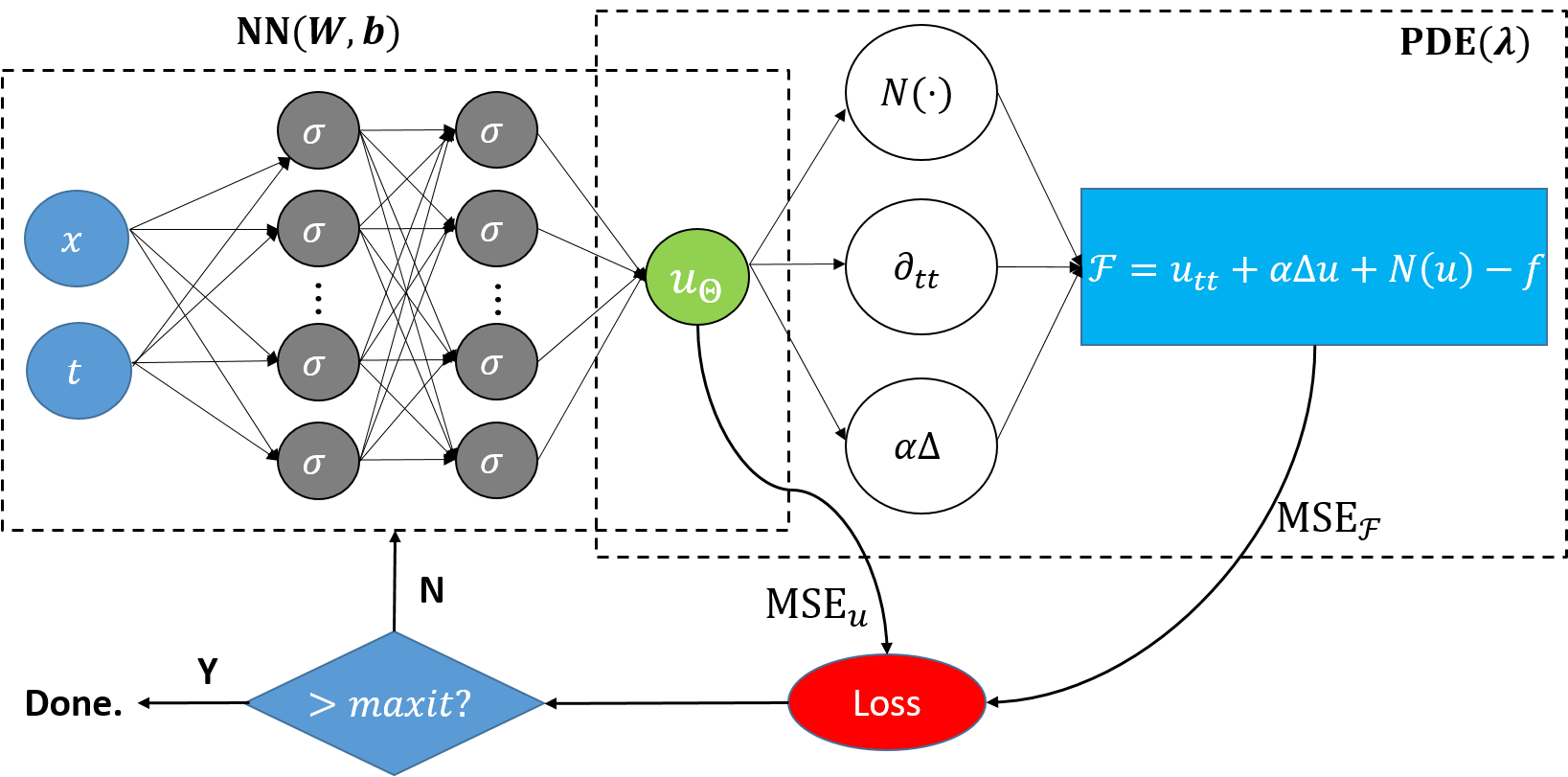
Figure 1: Schematic of PINN for the Klein-Gordon equation. The left (physics-uninformed) network represents the surrogate of the PDE solution $u_{\bm{\Theta}}(x,t)$ while the right (physics-informed) segment describes the PDE residual $\mathcal{F}=\frac{\partial^{2}u_{\bm{\Theta}}}{\partial t^{2}}+\alpha\Delta u_{\bm{\Theta}}+N(u_{\bm{\Theta}})-f$ calculation. The two parts share hyper-parameters, and they both contribute to the loss function. The loss function includes a supervised loss of data measurements of $u(x,t)$ from the initial and boundary conditions, namely, $\textnormal{MSE}_{u}$, and an unsupervised loss of PDE, namely, $\textnormal{MSE}_{\mathcal{F}}$.

PINN (Raissi et al.,, 2019) uses the NN structure in Eq. (2) to find the solution for the differential equation provided with the initial and boundary conditions. To demonstrate it, an example is presented in Figure 1 to solve the nonlinear Klein-Gordon equation using PINN. Klein-Gordon equation is a second-order hyperbolic partial differential equation arising in many scientific fields like soliton dynamics and condensed matter physics (Caudrey et al.,, 1975), solid-state physics, and nonlinear wave equations (Dodd et al.,, 1982). The in-homogeneous Klein-Gordon equation is given by

$$u_{tt}+\alpha\Delta u+N(u)=f(x,t),\ x\in[-1,1],\ t>0,$$ (3)

where $\Delta$ is a Laplacian operator and $N(u)=\beta u+\delta u^{k}$ is the nonlinear term with quadratic nonlinearity ($k=2$) and cubic non-linearity ($k=3$); $\lambda=\{\alpha,\beta,\delta\}$ are constants for the PDE. The initial and the boundary conditions are given by $u(x,0)=x$, $u(-1,t)=-\cos(t)$, and $u(1,t)=\cos(t)$. Specifically, the PINN algorithm aims to learn a NN surrogate $u_{\bm{\Theta}}$ for predicting the solution $u$ of the governing PDE as shown in Figure 1.

The NN solution must satisfy the governing equation given by the residual $\mathcal{F}(u_{\bm{\Theta}})=u_{{\bm{\Theta}}_{tt}}+\alpha\Delta u_{\bm{\Theta}}+N(u_{\bm{\Theta}})-f(x,t)$ evaluated at randomly chosen $N_{f}$ residual points in the domain which is used to calculate $\textnormal{MSE}_{\mathcal{F}}$ in Eq. (5). To construct the residuals in the loss function, derivatives of the solution $u_{\bm{\Theta}}$ with respect to the independent variables $x$ and $t$ are required, which can be computed using the Automatic Differentiation (AD) (Baydin et al.,, 2018). AD is an accurate way to calculate derivatives in a computational graph compared to numerical differentiation since they do not suffer from the errors such as truncation and round-off errors (Baydin et al.,, 2018). Thus, the PINN method is a grid-free method, which does not require mesh for solving equations, which is a popular approach used by Finite Element Method (Donea and Huerta,, 2003).

The main feature of the PINN is that it can easily incorporate all the given information (for example, governing equation, experimental data and initial/boundary conditions) into the loss function, thereby recast the original problem into an optimization problem. In the PINN algorithm, the loss function is defined as

$$J(\bm{\Theta})=w_{\mathcal{F}}\textnormal{MSE}_{\mathcal{F}}+w_{u}\textnormal{MSE}_{u},$$ (4)

where the mean squared error (MSE) is given as

$$\texttt{PDE residual loss: }\textnormal{MSE}_{\mathcal{F}} =\frac{1}{N_{f}}\sum_{i=1}^{N_{f}}\left|\mathcal{F}_{\bm{\Theta}}(\bm{x}_{f}^{i})\right|^{2},$$ (5)

$$\texttt{Data loss: }\textnormal{MSE}_{u} =\frac{1}{N_{u}}\sum_{i=1}^{N_{u}}\left|u(\bm{x}_{u}^{i})-u_{\bm{\Theta}}(\bm{x}_{u}^{i})\right|^{2},$$ (6)

where $\{\bm{x}_{f}^{i}\}_{i=1}^{N_{f}}$ represents the set of $N_{f}$ residual points and $\{\bm{x}_{u}^{i}\}_{i=1}^{N_{u}}$ represents the set of $N_{u}$ training data points. $w_{\mathcal{F}}>0$ and $w_{u}>0$ are the weights for residual and training data points, respectively, which are user-defined or tuned automatically (Wang et al.,, 2021). Specifically, we have

• PDE residual loss in Eq. (5) (i.e., the first term in Eq. (4)) enforces the NN solution $u_{\bm{\Theta}}$ to obey the PDE. If the dimension of $\bm{x}$ is one, it is an ordinary differential equation (ODE);

• Data loss in Eq. (6) (i.e., the second term in Eq. (4)) includes the known initial/boundary conditions and/or experimental data, which must be satisfied by the NN solution $u_{\bm{\Theta}}$.

The resulting optimization problem is to find the minimum of the loss function by optimizing the parameters, i.e., we seek to find

$$\bm{\Theta}^{*}=\underset{\bm{\Theta}}{\arg\min}\ J(\bm{\Theta}).$$ (7)

The solution to problem (7) can be approximated iteratively by one of the forms of gradient descent algorithm, such as Adam (Kingma and Ba,, 2014) and L-BFGS (Byrd et al.,, 1995).

2.2 Self-scalable Tanh Activation Function

The role of an activation function is to induce non-linearity into the NN model. It is well known that NN with a non-polynomial activation function can model any function (Leshno et al.,, 1993). The nonlinear activation function performs the nonlinear transformation to the input data, making it capable of learning and performing more complex tasks. In general, the activation functions need to be differentiable so that the back-propagation is possible, where the gradients are supplied to update the weights and biases.

In PINN, the activation function also plays a role in finding the derivatives (for example, $\frac{du_{\bm{\Theta}}}{dx}$ to find PDE residual loss). As mentioned previously, non-smooth activation functions are not suitable for the PINN task (Mishra and Molinaro,, 2020). The tanh and its adaptive modification (Jagtap et al., 2020b, ; Jagtap et al., 2020a, ) remain the most sought-after activation function for PINN  (Jagtap et al., 2020c, ; Jagtap and Karniadakis,, 2020; Singh et al.,, 2019; Zhang and Gu,, 2021). Eq. (8) gives the widely used tanh function (LeCun et al.,, 2012) as

$$\textnormal{tanh}(x)=\frac{e^{x}-e^{-x}}{e^{x}+e^{-x}}.$$ (8)

tanh has several advantages including continuity and differentiability providing smooth gradient over the entire support (LeCun et al.,, 2012). However, in the context of PINN, there are two main issues for the widely used tanh-based activation functions:

$\bullet$ The first one is that PINN is more likely to have the problem of vanishing gradients due to the calculation of PDE residual loss. The vanishing gradients are caused by the saturation of the activation function, which has the following definition.

Definition 1 (Saturation (Gulcehre et al.,, 2016)).

An activation function $\sigma(x)$ with derivative $\sigma^{\prime}(x)$ is said to right (resp. left) saturate if its limit as $x\to+\infty$ (resp. $x\to-\infty$) is zero. An activation function is said to saturate (without qualification) if it both left and right saturates.

For example, $\mathcal{F}_{\bm{\Theta}}$ at a particular $x_{f}^{i}$ can be calculated by computing the derivative (i.e., $\frac{du_{\bm{\Theta}}}{dx}|_{x=x_{f}^{i}}$) for any given problem (refer to Section 4) by AD. This is done by using the chain rule of differentiation considering the NN weights and biases as constant. With the notation introduced in Section 2.1 and some simplification of it for clarity, the expression for the required derivative can be roughly given as

$$\frac{du_{\bm{\Theta}}}{dx}\Bigg{|}_{x=x_{f}^{i}}=\Bigg{[}\frac{\partial\mathcal{L}_{D}}{\partial z_{D-1}}\times\frac{\partial z_{D-1}}{\partial\mathcal{L}_{D-1}}\times\frac{\partial\mathcal{L}_{D-1}}{\partial z_{D-2}}\times\cdots\times\frac{\partial z_{1}}{\partial\mathcal{L}_{1}}\times\frac{\partial\mathcal{L}_{1}}{\partial x}\Bigg{]}\Bigg{|}_{x=x_{f}^{i}},$$ (9)

which is very similar to the back-propagation that includes the gradient of activation functions at each layer (i.e., $\frac{\partial z_{k}}{\partial\mathcal{L}_{k}}$). The derivative in Eq. (9) is a part of PDE residual loss, where the gradient of PDE residual loss with respect to weights and biases of PINN (i.e., $\frac{\partial\textnormal{MSE}_{\mathcal{F}}}{\partial\bm{\Theta}})$ is calculated by back-propagation (Lagaris et al.,, 1998; Goodfellow et al.,, 2016). This makes PINN have a “deeper” structure, to calculate the gradients of parameters, than standard neural networks. Thus, PINN is more likely to suffer from vanishing gradients caused by saturation (Wang et al.,, 2021). It is theoretically analyzed by Wang et al., (2021) that vanishing gradients can lead to a concentration of training gradients around zero for optimizing the PDE residual loss. The problem gets even more troublesome when higher-order derivatives and larger dimensional equations are solved.

$\bullet$ The second issue is the unstable training due to the requirement of varied magnitudes of weights. The output from tanh (or the adaptive version) is bounded between -1 and 1. When using tanh for regression problems, it is well known that the last layer should be linear to allow the output to take any value and not constrained by the activation function (Mathew et al.,, 2020). When the output is not normalized, it can lead to unstable training (Ranjan,, 2020; Bishop et al.,, 1995). As already introduced in Section 1, the output from PINN can not be normalized since the magnitude is not known with the PDE and initial/boundary conditions. This implies, for an accurate model with tanh activation, the penultimate layer has an output between -1 and 1, but the final layer’s output should be of the appropriate range (possibly high). This further implies that the last layer weights should be higher in magnitude than the rest of the layers. This complicates the training (Bishop et al.,, 1995) for both tanh function and its adaptive modification. It is preferred that the model gradually scales into different orders of magnitude than just using the last layer for scaling up.

Both of the mentioned issues are more pronounced when the outputs are of higher orders of magnitude. Therefore, to address these two issues

• First, there is a need for higher gradients and non-saturation behaviour for activation functions;

• Second, the activation function should be unbounded.

Accordingly, the proposed Self-scalable tanh (Stan) activation function for $i$th neuron in $k$th layer ($k=1,2,\dots,D-1;\ i=1,2,\dots,N_{k}$) is proposed as

$$\sigma^{i}_{k}(x)=\textnormal{tanh}(x)+\beta^{i}_{k}x\cdot\textnormal{tanh}(x),$$ (10)

where $\beta^{i}_{k}$ is the neuron-wise parameter that should be optimized. The second term, namely, $\beta^{i}_{k}x\cdot\textnormal{tanh}(x)$, is the self-scaling term that can help to better map different orders of magnitude of input and output when allowing the gradients to flow without vanishing. Figure 2 shows the visualization of Stan activation and its gradient.

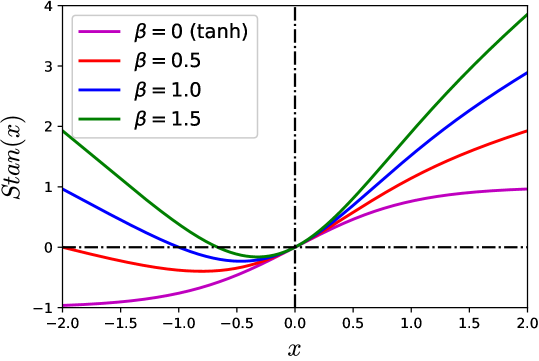
(a) Stan activation function

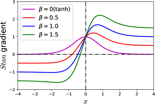
(b) Stan activation function gradient

Figure 2: Visualization of the proposed Stan activation function in comparison with tanh. At $x=0$, the function value is 0 and the gradient is 1. The point of zero gradient and maximum gradient are dependent on $\beta$.

From Figure 2b, our proposed Stan activation function does not have the saturation problem, which can be formally quantified in the following proposition.

Proposition 2.

If $\beta^{i}_{k}\neq 0$, the proposed activation function in (10) is not saturation.

Proof.

The first-order derivative of $\sigma^{i}_{k}(x)$ is

$$(\sigma_{k}^{i})^{\prime}(x)=(1+\beta^{i}_{k}x)\Big{(}1-\textnormal{tanh}^{2}(x)\Big{)}+\beta^{i}_{k}\textnormal{tanh}(x).$$

Therefore, we have

$$\lim_{x\to+\infty}(\sigma^{i}_{k})^{\prime}(x) =\beta^{i}_{k},$$

$$\lim_{x\to-\infty}(\sigma^{i}_{k})^{\prime}(x) =-\beta^{i}_{k}.$$

∎

The proposed Stan gives additional $\sum_{k=1}^{D-1}N_{k}$ parameters to be optimized. In this case, we have $\tilde{\bm{\Theta}}=\{\bm{W}^{k},\bm{b}^{k}\}_{k=1}^{D}\bigcup\{\bm{\beta}^{k}\}_{k=1}^{D-1}$ are trainable parameters, where $\bm{\beta}^{k}=(\beta_{k}^{1},\beta_{k}^{2},\dots,\beta_{k}^{N_{k}})^{\top}$. The parameter $\tilde{\bm{\Theta}}$ is updated as

$$\tilde{\bm{\Theta}}_{m+1}=\tilde{\bm{\Theta}}_{m}-\eta_{m}\nabla J(\tilde{\bm{\Theta}}_{m}),$$ (11)

where $\eta_{m}\in(0,1]$ is the learning rate at $m$th iteration. The proposed activation function-based PINN algorithm is summarized in Algorithm 1.

Algorithm 1 Self-scalable tanh activation function-based PINN algorithm

Input: Training data: $u_{\tilde{\bm{\Theta}}}$ network $\{\bm{x}_{u}^{i}\}_{i=1}^{N_{u}}$; Residual training points: $\{\bm{x}_{f}^{i}\}_{i=1}^{N_{f}}$

Step 1: Construct neural network $u_{\tilde{\bm{\Theta}}}$ with random initialization of parameters $\tilde{\bm{\Theta}}$.

Step 2: Construct the residual $\mathcal{F}_{\tilde{\bm{\Theta}}}$ of neural network by substituting surrogate $u_{\tilde{\bm{\Theta}}}$ into the governing equation using automatic differentiation and other arithmetic operations.

Step 3: Specification of loss function:

$$J(\tilde{\bm{\Theta}})=\frac{w_{\mathcal{F}}}{N_{f}}\sum_{i=1}^{N_{f}}\left|\mathcal{F}_{\tilde{\bm{\Theta}}}(\bm{x}_{f}^{i})\right|^{2}+\frac{w_{u}}{N_{u}}\sum_{i=1}^{N_{u}}\left|u^{i}-u_{\tilde{\bm{\Theta}}}(\bm{x}_{u}^{i})\right|^{2}.$$ (12)

Step 4: Find the best parameters $\tilde{\bm{\Theta}}^{*}$ using a suitable optimization method for minimizing the loss function in (12) as

$$\tilde{\bm{\Theta}}^{*}=\underset{\tilde{\bm{\Theta}}}{\arg\min}\ J(\tilde{\bm{\Theta}}).$$

Output: $u_{\tilde{\bm{\Theta}}^{*}}$ network

We now provide a theoretical result regarding the PINN with the proposed Stan. The following theorem states that a gradient descent algorithm minimizing our objective function in Eq. (12) with a L2 regularization term does not converge to a spurious stationary point given appropriate initialization and learning rates. Now, let $J_{\gamma}(\tilde{\bm{\Theta}})\coloneqq J_{\gamma}(\tilde{\bm{\Theta}})+\gamma\|B\|_{2}^{2}$ (i.e., the objective function in Eq. (12) with the L2 regularization) where $B\coloneqq\{\bm{\beta}_{k}\}_{k=1}^{D-1}$, $\gamma>0$ is a fixed hyper-parameter that can be defined by users.

Theorem 3 (No Spurious Stationary Points).

Let $\{\tilde{\bm{\Theta}}_{m}\}_{m\geq 0}$ be a sequence generated by a gradient descent algorithm based on the update rule in Eq. (11). Assume that $J_{\gamma}(\tilde{\bm{\Theta}}_{0})<J_{\gamma}(\bm{0})$, $J_{\gamma}$ is differentiable, and that for each $i\in\{1,\dots,N_{f}\}$, there exist a differentiable function $\phi^{j}$ and input $\rho^{j}$ such that $\left|\mathcal{F}(\bm{x}_{f}^{j})\right|^{2}=\phi^{j}(u_{\tilde{\bm{\Theta}}}(\rho^{j}))$, another differentiable function $\pi^{i}_{k}$ so that $\sigma^{i}_{k}(x)=\pi^{i}_{k}(\beta^{i}_{k}x)$ for all $i,k$. Suppose one of the following conditions holds:

1. $\nabla J_{\gamma}(\tilde{\bm{\Theta}})$ is Lipschitz continuous with Lipschitz constant $C>0$. That is, $\|\nabla J_{\gamma}(\tilde{\bm{\Theta}})-\nabla J_{\gamma}(\tilde{\bm{\Theta}}^{\prime})\|_{2}\leq C\|\tilde{\bm{\Theta}}-\tilde{\bm{\Theta}}^{\prime}\|_{2}$ for all $\tilde{\bm{\Theta}},\tilde{\bm{\Theta}}^{\prime}$ in its domain. And $\varepsilon\leq\eta_{m}\leq\frac{2-\varepsilon}{C}$, where $\varepsilon>0$ is a fixed positive number;

2. $\nabla J_{\gamma}(\tilde{\bm{\Theta}})$ is Lipschitz continuous, $\eta_{m}\to 0$, and $\sum_{m=1}^{+\infty}\eta_{m}=+\infty$;

3. The learning rate $\eta_{m}$ is chosen by the minimization rule, the limited minimization rule, the Armjio rule, or the Goldstein rule (Bertsekas,, 1997).

Then, no limit point of $\{\tilde{\bm{\Theta}}_{m}\}_{m\geq 0}$ is a spurious stationary point.

Proof.

See proof in Appendix A. ∎

The initial condition $J_{\gamma}(\tilde{\bm{\Theta}}_{0})<J_{\gamma}(\bm{0})$ means that the initial value $J_{\gamma}(\tilde{\bm{\Theta}}_{0})$ needs to be less than that of a constant network. This analysis is not possible without introducing the $\{\bm{\beta}_{k}\}_{k=1}^{D-1}$ in the proposed activation function. The above Theorem 3 shows that if the algorithm converges to a stationary point, it converges to global optimal solutions under three independent conditions. The conditions (i), (ii), and (iii) correspond to the cases of the constant learning rate, diminishing learning rate, and adaptive learning rate, respectively. For our experiments in Sections 3 and 4, the constant learning rate is adopted. The training loss from these experiments, which usually converge to zero, illustrates that the algorithm can escape the problem of Spurious Local Minima (Safran and Shamir,, 2018) in neural networks.

3 Numerical Study

In Section 3.1, nonlinear smooth and discontinuous functions used in Jagtap et al., 2020b are used to verify the effectiveness of the proposed activation function, namely, Stan. The sensitivity analysis on the initialization of $\beta^{i}_{k}$s is presented in Section 3.2. In all analyses, tanh and Neuron-wise Locally Adaptive Activation Function (N-LAAF) Jagtap et al., 2020a are selected as benchmarks for comparison with the proposed activation function, which are state-of-the-art activation functions for PINN. N-LAAF is an adaptive modification of the tanh function by introducing an adaptive parameter $a^{i}_{k}$ for every neuron as $\textnormal{tanh}(a^{i}_{k}x)$. For this numerical study, the same setup in (Jagtap et al., 2020b, ) is used, where the neural network architecture consists of four hidden layers with 50 neurons in each layer, and Adam optimizer (learning rate 0.0008) is utilized for training. All the results are repeated ten times with different initializations of NN weights and biases to obtain the average performance. The codes of all the experiments are implemented in Python 3 with Pytorch 1.9.0 package. The GPU used in this work is an NVIDIA 2080 Ti.

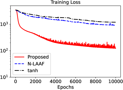
(a) Empirical convergence of training loss

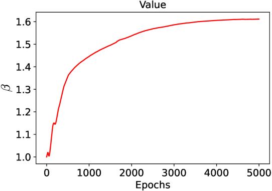
(b) Empirical convergence of $\beta^{i}_{k}$ in one of the neurons

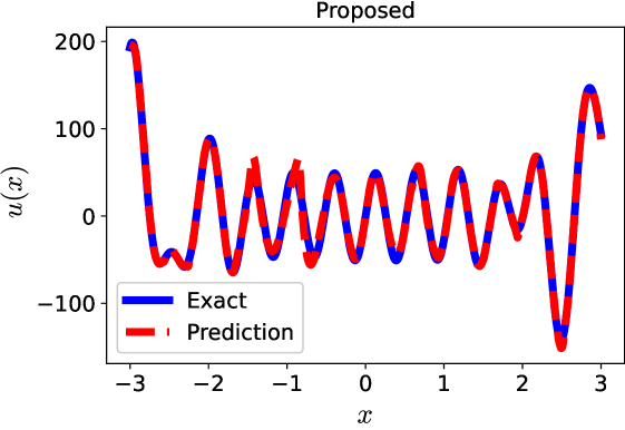
(c) Neural network solution of the proposed method

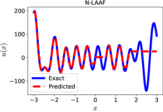
(d) Neural network solution of N-LAAF

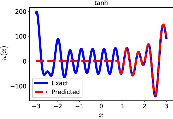
(e) Neural network solution of tanh

Figure 3: Results of the smooth function: (a) Empirical convergence of training loss; (b) Empirical convergence of $\beta^{i}_{k}$; (c) Neural network solution of the proposed method; (d) Neural network solution of N-LAAF; (e) Neural network solution of tanh.

3.1 Neural Network Approximation of Functions

In this subsection, a standard NN (without the physics-informed part) is employed to approximate smooth and discontinuous functions. Specifically, the smooth and discontinuous functions defined by Jagtap et al., 2020b are scaled with a constant factor given as

$$u(x)=50\times\Big{[}(x^{3}-x)\frac{\sin(7x)}{7}+\sin(12x)\Big{]},\,\,x\in[-3,3],$$ (13)

and

$$u(x)=\Bigg{\{}\begin{split}40\sin(6x),\,\,-4&\leq x\leq 0\\ 200+20x\cos(12x),\,\,0&<x\leq 3.75.\\ \end{split}$$ (14)

300 randomly sampled points with their corresponding $u(x)$ values are used to train the model and 1,000 evenly spaced points for testing. The output data is not normalized to test the effectiveness of the proposed activation function. The parameters $\beta^{i}_{k}$s are initialized with the value 1. The loss function for this case is the mean squared error of prediction on the training data as given below

$$\textnormal{MSE}_{u}=\frac{1}{300}\sum_{i=1}^{300}\left|u(x^{i}_{u})-u_{\tilde{\bm{\Theta}}}(x^{i}_{u})\right|^{2}.$$

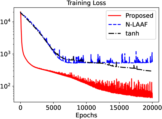
(a) Empirical convergence of training loss

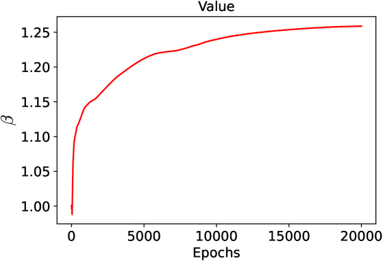
(b) Empirical convergence of $\beta^{i}_{k}$ in one of the neurons

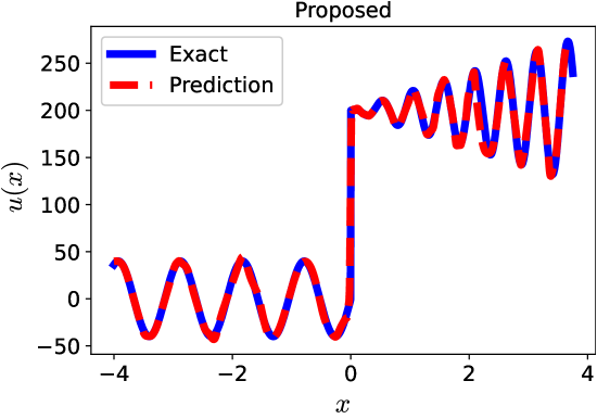
(c) Neural network solution of the proposed method

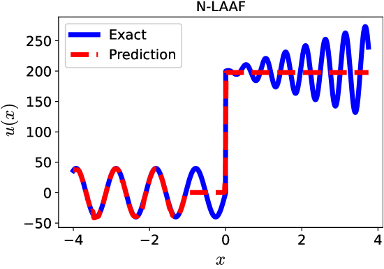
(d) Neural network solution of N-LAAF

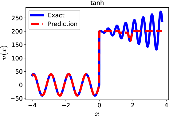
(e) Neural network solution of tanh

Figure 4: Results of the discontinuous function: (a) Empirical convergence of training loss; (b) Empirical convergence of $\beta^{i}_{k}$; (c) Neural network solution of the proposed method; (d) Neural network solution of N-LAAF; (e) Neural network solution of tanh.

The results are summarized in Figures 3 and 4. Figure 3a shows the training performance of the smooth function with the proposed activation compared to benchmark methods. After 10,000 epochs, the proposed method shows significantly better training loss than other benchmark methods. The convergence of $\beta_{k}^{i}$ in one of the randomly chosen neurons is shown in Figure 3b. For that particular $\beta^{i}_{k}$, the value converges to around $1.6$ with almost a similar rate as the training loss.

Figures 3c, 3d and 3e show the model prediction of different methods in the testing phase. The proposed method is the only one that can perfectly fit the function in Eq. (13), while other methods have a poor fitting. Figure 4a similarly shows the training performance of the discontinuous function for 20,000 epochs. The convergence of $\beta_{k}^{i}$ (to around $1.25$) in one of the neurons is also shown in Figure 4b. Figures 4c, 4d and 4e show that our proposed method performs best for model prediction among all methods.

Table 1: Test performance of function approximation for different methods in terms of MSE and RE.

	tanh		N-LAAF		Proposed
	MSE	RE	MSE	RE	MSE	RE
Eq. (13)	1369.60	0.6249	988.18	0.5308	185.46	0.2299
Eq. (14)	47.77	0.1930	37.32	0.1706	23.97	0.1367

In addition, the test performance for different methods in terms of MSE and RE (relative error) (Raissi et al.,, 2019; Jagtap et al., 2020b, ) is summarized in Table 1. The proposed method achieves the best performance for both functions in Eqs. (13) and (14) in terms of MSE and RE. The better performance in these two cases can be attributed mainly to the second issue discussed in Section 2.2.

3.2 Sensitivity Analysis

This study is focused on the activation function and the proposed activation function has trainable parameters $\beta_{k}^{i}$s. For the case studies in 3.1, these values are initialized as 1. In this subsection, the sensitivity analysis is conducted concentrating on the initialization of these $\beta_{k}^{i}$s. Specifically, for both the functions used in Section 3.1, all $\beta_{k}^{i}$s are initialized from ten values, which are equally spaced in the range $[0.25,1.15]$.

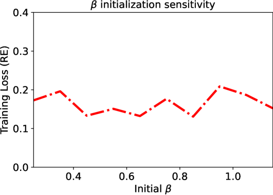
(a) Smooth Function

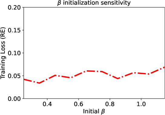
(b) Discontinuous Function

Figure 5: Sensitivity of training under various initialization of $\beta^{i}_{k}$. Note that $\beta^{i}_{k}$s are initialized with the same value for all the neurons, $\beta$ is used to represent the value.

The training losses from the last epoch for both functions (averaged over ten repetitions) in terms of RE are plotted in Figure 5 with different initialization of $\beta_{k}^{i}$s. The results show that our proposed Stan is very stable training with different initialization of $\beta_{k}^{i}$s, which is particularly desired for more involved PINN case studies in Section 4.

4 Forward and Inverse Problems using PINN

In this Section, the proposed Stan activation is tested on the multiple problems involving differential equations. These problems can be summarized into two types: (1) forward problem in Section 4.1, where the problem is to identify the solution of given a differential equation with its corresponding initial/boundary conditions (2) inverse problem in Section 4.2, where the problem is to discover the coefficients of the differential equation given the solution. L-BFGS optimizer with the default learning rate 1 is used for all the cases in this section to evaluate the performance. All the results are repeated ten times with different initializations of NN weights and biases to obtain the average performance.

4.1 Forward Problem

4.1.1 1-Dimensional Problems

As described in Section 2.1, given a specific form of the differential equation, the task of PINN is to solve the differential equation with the given initial/boundary conditions. The data provided to the NN is those on the boundary. A NN of nine hidden layers with 50 neurons in each layer is utilized. The parameters $\beta^{i}_{k}$s are initialized with the value 1. Here, the first example considered is a second-order ODE as

$$\frac{d^{2}u}{dx^{2}}+\frac{du}{dx}=6u,\,\,x\in[0,2],$$ (15)

$$u(0)=2,\,\,\frac{du}{dx}|_{x=0}=-1,$$

where there is a single point boundary (Dirichlet boundary) at the left end, namely, $x^{1}_{u}=0$, and a first derivative boundary (Neumann boundary) at the same end. The differential equation residual $\mathcal{F}_{\bm{\Theta}}$ needs to be zero for all points in the support. To enforce this condition, a set of 1,000 points ($x^{i}_{f},i=1,2,\dots,1000$) are selected randomly for every training epoch. Therefore, the loss is calculated by adding the loss of all the boundary conditions and the ODE residuals as in Eq. (16),

$$J(\tilde{\bm{\Theta}})=\frac{w_{\mathcal{F}}}{1000}\sum_{i=1}^{1000}\left|\mathcal{F}_{\tilde{\bm{\Theta}}}(x_{f}^{i})\right|^{2}+w_{u}\left|u(0)-u_{\tilde{\bm{\Theta}}}(0)\right|^{2}+w_{g}\left|\mathcal{G}_{\tilde{\bm{\Theta}}}(0)\right|^{2},$$ (16)

where $\mathcal{G}_{\tilde{\bm{\Theta}}}(x^{1}_{g})=\frac{du_{\tilde{\bm{\Theta}}}}{dx}|_{x=x^{1}_{g}}-\frac{du}{dx}|_{x=x^{1}_{g}}$ is an additional loss term corresponding to the Neumann boundary condition at $x^{1}_{g}=0$ in Eq. (15). $\mathcal{F}_{\tilde{\bm{\Theta}}}(x_{f}^{i})$ takes the following form

$$\mathcal{F}_{\tilde{\bm{\Theta}}}(x^{i}_{f})=\frac{d^{2}u_{\tilde{\bm{\Theta}}}}{dx^{2}}|_{x=x^{i}_{f}}+\frac{du_{\tilde{\bm{\Theta}}}}{dx}|_{x=x^{i}_{f}}-6u_{\tilde{\bm{\Theta}}}(x^{i}_{f}),\,\,i=1,2,\dots,1000.$$

For this case, the weights $w_{f},w_{u}$, and $w_{g}$ are taken as $1$.

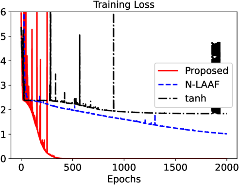
(a) Empirical convergence of training loss

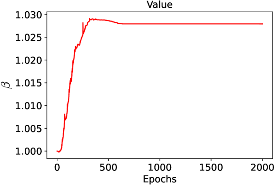
(b) Empirical convergence of $\beta^{i}_{k}$ in one of the neurons

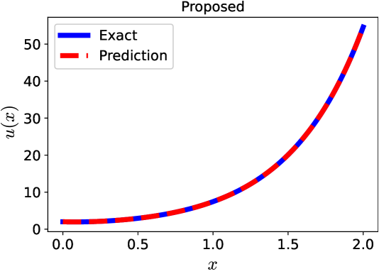
(c) Neural network solution of the proposed method

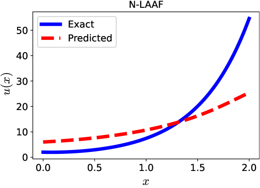
(d) Neural network solution of N-LAAF

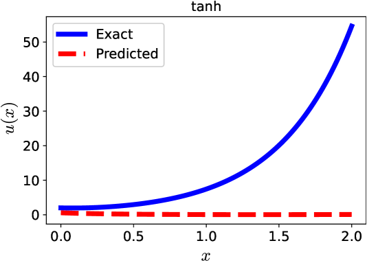
(e) Neural network solution of tanh

Figure 6: Results of Solving Eq. (15): (a) Empirical convergence of training loss; (b) Empirical convergence of $\beta^{i}_{k}$; (c) Neural network solution of the proposed method; (d) Neural network solution of N-LAAF; (e) Neural network solution of tanh.

As shown in Figure 6a, the average loss in Eq. (16) converges to zero for the proposed activation function while other methods cannot. The convergence of $\beta_{k}^{i}$ in one of the neurons is shown in Figure 6b. It is well known that the problem in Eq. (15) has a closed-form solution $u(x)=e^{2x}+e^{-3x},\,\,x\in[0,2]$. The results of the neural network solution of Eq. (15) are summarized in Figures 6c, 6d, and 6e. Our proposed method is the only one that can achieve the exact solution. Though this problem is simple, one-dimensional, and analytically solvable, the PINNs with tanh and N-LAAF activation functions fail to give an accurate NN model for this function. This is mainly due to the difference in scale between $x$, which is $[0,2]$, and $u$, which is approximately $[0,55]$. Also, note that, with the given problem in Eq. (15), there is no way to identify the scale of $u$. The activation function N-LAAF, though improves the training, does not predict an accurate solution either.

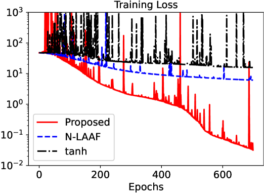
(a) Empirical convergence of training loss

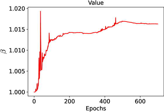
(b) Empirical convergence of $\beta^{i}_{k}$ in one of the neurons

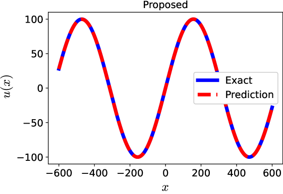
(c) Neural network solution of the proposed method

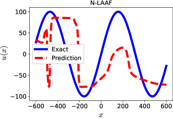
(d) Neural network solution of N-LAAF

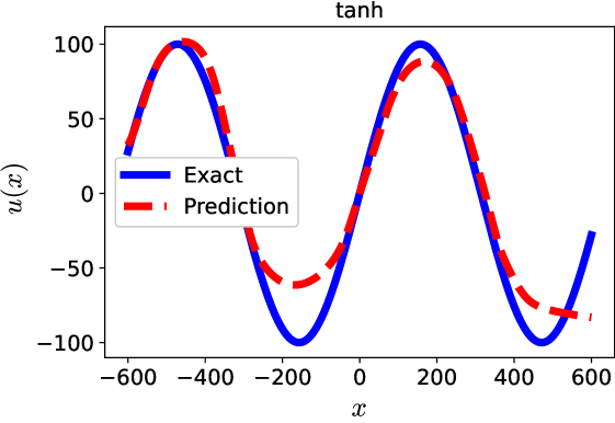
(e) Neural network solution of tanh

Figure 7: Results of solving Eq. (17): (a) Empirical convergence of training loss; (b) Empirical convergence of $\beta^{i}_{k}$; (c) Neural network solution of the proposed method; (d) Neural network solution of N-LAAF; (e) Neural network solution of tanh.

The second 1D example considered is inspired by the motivating example by Moseley et al., (2021). Moseley et al., (2021) used a domain decomposition-based approach to address the spectral bias in the PINN methods. Unlike the first case, this is a first-order ODE with a single boundary condition as below

$$\begin{split}&\frac{du}{dx}=\cos(\omega x),\,\,x\in[-600,600],\\ &u(0)=0.\end{split}$$ (17)

Specifically, the problem is considered with very low frequency ($\omega=0.01$). The loss function follows the formulation presented in Eq. (12) as restated for this problem as

$$J(\tilde{\bm{\Theta}})=\frac{w_{\mathcal{F}}}{10000}\sum_{i=1}^{1000}\left|\mathcal{F}_{\tilde{\bm{\Theta}}}(\bm{x}_{f}^{i})\right|^{2}+w_{u}\left|u(0)-u_{\tilde{\bm{\Theta}}}(0)\right|^{2},$$ (18)

where $\mathcal{F}_{\tilde{\bm{\Theta}}}(x^{i}_{f})=\frac{du_{\tilde{\bm{\Theta}}}}{dx}|_{x^{i}_{f}}-\cos(0.01x^{i}_{f})$. The weights $w_{\mathcal{F}}$ and $w_{u}$ are chosen as 100 and 1, respectively, and 10,000 residual points are chosen randomly for every epoch.

The problem in Eq. (17) has the solution of the form $u(x)=100\sin(0.01x)$, where the magnitude of $u$ is in the order of $10^{2}$. Figure 7 shows the algorithm convergence and prediction performance of the proposed method in comparison with the benchmark methods. As shown in Figure 7a, the proposed activation function is the only method that can achieve zero average loss in Eq. (18). In Figure 7c, the neural network solution of the proposed method can exactly match the solution. As seen in Figures 7d and 7e, N-LAAF is the worst in predicting the solution even though its training loss (as shown in Figure 7a) is better than the tanh activation.

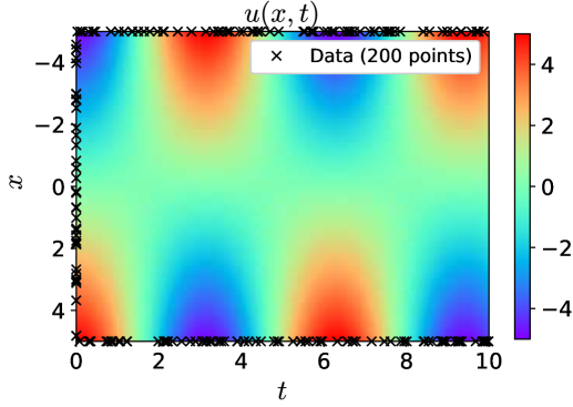
Figure 8: Ground truth solution of the Klein-Gordon equation. 200 “$\times$”s are shown as training data for visualization purpose.

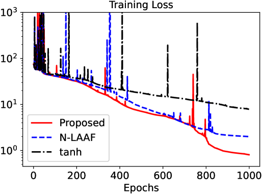
(a) Empirical convergence of training loss

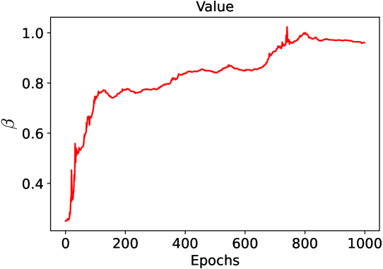
(b) Empirical convergence of $\beta^{i}_{k}$ in one of the neurons

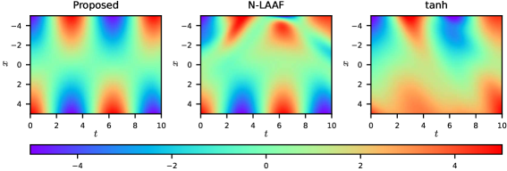
(c) Neural network solutions of the proposed method, N-LAAF, and tanh

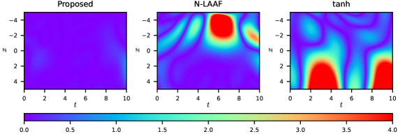
(d) Absolute error maps for neural network solutions of the proposed method, N-LAAF, and tanh

Figure 9: Results of the Klein-Gordon equation: (a) Empirical convergence of training loss; (b) Empirical convergence of $\beta^{i}_{k}$; (c) Neural network solutions of the proposed method, N-LAAF, and tanh; (d) Neural network solution of N-LAAF; (e) Absolute error maps for neural network solutions of the proposed method, N-LAAF, and tanh.

4.1.2 2-Dimensional Problem

As described in Section 2, the Klein-Gordon equation is a second-order partial differential equation (Caudrey et al.,, 1975) arising in many branches of physics. The inhomogeneous Klein-Gordon equation, as given in Eq. (3), is used in this case study with the conditions given in Jagtap et al., 2020b but for an extended domain (i.e., $x\in[-5,5]$) and the same time interval (i.e., $t\in[0,10]$). Specifically, the exact problem considered is given by

$$\begin{split}&\frac{\partial^{2}u}{\partial t^{2}}-\frac{\partial^{2}u}{\partial x^{2}}+u^{2}=-x\cos(t)+x^{2}\cos^{2}(t),\,\,x\in[-5,5],t>0,\\ &u(x,0)=x;\,\,u(-5,t)=-5\cos(t);\,\,u(5,t)=5\cos(t).\\ \end{split}$$ (19)

The above problem in Eq. (19) has a closed-form solution given by $u(x)=x\cos(t),\,\,x\in[-5,5]$ as shown visually in Figure 8. For the purpose of training, 500 points are chosen randomly on the boundaries (comprising of all the points where $x=-5$ or $x=5$ or $t=0$) for the Data loss in Eq. (6). 10,000 residual points are randomly chosen from the support domain for the PDE loss in Eq. (5). The neural network architecture used for this case study consists of nine hidden layers with 50 neurons in each layer. All $\beta_{k}^{i}$s are initialized with 0.25 and weights $w_{f},w_{u}$ are taken as 1.

Figure 9 summarizes the convergence and prediction performance of different methods. Figure 9a shows that our approach has a similar convergence speed with N-LAAF for the first 800 epochs but converges to a better solution in the end. Figures 9c and 9d correspond to the neural network solutions and absolute error maps for different methods. It can be observed visually that the proposed method outperforms the benchmark methods. On the other hand, N-LAAF has better convergence than the tanh activation. This case study illustrates that even without changing any coefficients/parameters of Klein-Gordon equation from Jagtap et al., 2020b , simply by extending the domain (from $x\in[-1,1]$ to $x\in[-5,5])$, the output can be of higher magnitudes and the benchmark methods fail to scale up.

4.2 Inverse Problem

Another significant problem related to PINN is the inverse problem, which is to find the differential equation itself with the given data Raissi et al., (2019). Specifically, it aims to find the coefficients/parameters of the differential equation, which is also called the data-driven discovery of partial differential equations. This problem is encountered practically in many cases. For instance, sensor data can be used to calculate the material property or characteristic of a given work-piece (Harrsion et al.,, 2020; Crawford et al.,, 2018).

To demonstrate the effectiveness of the proposed activation function in the inverse problem, the transient heat transfer in a rod is considered (Cengel,, 2008). The rod is considered one-dimensional with a length of one unit. It has a constant initial temperature of $u_{0}$ and starts to cool down at time $t=0$. The ends of the rod are assumed to be maintained at a temperature of zero units. Thermal effects except the conduction are ignored. Specifically, the conduction heat transfer equation (Cengel,, 2008) given by the PDE with initial and boundary conditions, where $u(x,t)$ is the temperature that follows

$$\begin{split}\texttt{PDE}&:\,\,\frac{\partial u}{\partial t}=\kappa\frac{\partial^{2}u}{\partial x^{2}},\,\,0<x<1,\\ \texttt{Initial Condition}&:\,\,u(x,0)=u_{0},\,\,0<x<1,\\ \texttt{Boundary Condition}&:\,\,u(0,t)=u(1,t)=0,\,\,t>0,\end{split}$$ (20)

where the thermal diffusivity $\kappa$ is a constant for a given rod. In this case, it is assumed that the $\kappa$ is unknown. The goal is to find the thermal diffusivity of the rod (i.e., $\kappa$) based on the thermal measurement at specific points during the transition to equilibrium temperature. From the physics perspective and/or the PINN perspective, the objective is to identify the coefficient of the differential equation denoted as $\kappa$ (i.e., the thermal diffusivity) given the approximate temperature data (i.e., $\bar{u}(x,t)$) spread over the entire domain. In addition, PINN can produce a better approximation (i.e., $u_{\bm{\Theta}}(x,t)$) of the temperature distribution (i.e., solution $u(x,t)$) for the rod as a function of spatial location $x$ and time $t$.

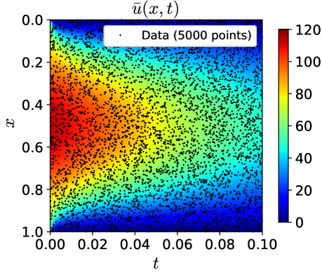
Figure 10: Approximate solution of the transient 1D Heat Transfer equation calculated by closed-form expression. The “$\cdot$”s represent training data.

To simulate this case, the thermal diffusivity $\kappa^{*}=1$ is considered the ground truth and the initial temperature $u_{0}$ of the rod is set as 50 units. By choosing $\kappa^{*}=1$, it leads to sufficient cooling within $t=0.1$ units. Therefore, the data within that time interval is sufficient to consider cooling. For this particular case, the analytical solution (Cengel,, 2008) is given by an infinite series as

$$u(x,t)=\frac{4u_{0}}{\pi}\sum_{i=1}^{\infty}\frac{\sin\Big{(}(2i-1)\pi x\Big{)}}{2i-1}\exp{\Big{(}-(2i-1)^{2}\pi^{2}t\Big{)}}.$$ (21)

Choosing any finite number of terms from the infinite series results in an approximation $\bar{u}(x,t)$ of the actual function $u(x,t)$. In this work, the first 10,000 terms of the series were used to calculate the approximation $\bar{u}(x,t)$, which is accurate enough (Cengel,, 2008). 5,000 randomly chosen spatial-temporal locations from $0\leq x\leq 1,0\leq t\leq 0.1$, and their corresonding $\bar{u}(x,t)$ are treated as thermal measurement data for training. The visualization of the approximate solution and thermal measurement data is shown in Figure 10.

To find the thermal diffusivity $\kappa$, the loss function is based on the one in Eq. (12) with an additional trainable parameter $\kappa$ in the residual part, which has the following form.

$$J(\tilde{\bm{\Theta}},\kappa)=\frac{w_{\mathcal{F}}}{50000}\sum_{i=1}^{50000}\left|\mathcal{F}_{\tilde{\bm{\Theta}},\kappa}(\bm{x}_{f}^{i})\right|^{2}+\frac{w_{u}}{5000}\sum_{i=1}^{5000}\left|\bar{u}^{i}(\bm{x}_{u}^{i})-u_{\tilde{\bm{\Theta}}}(\bm{x}_{u}^{i})\right|^{2},$$ (22)

where $\mathcal{F}_{\tilde{\bm{\Theta}},\kappa}(\bm{x}_{f}^{i})=\frac{\partial u_{\tilde{\bm{\Theta}}}}{\partial t}|_{\bm{x}_{f}^{i}}-\kappa\frac{\partial^{2}u_{\tilde{\bm{\Theta}}}}{\partial x^{2}}|_{\bm{x}_{f}^{i}}$, $w_{u}=w_{\mathcal{F}}=1$, and a set of 50,000 points are used as residual points to ensure the PDE is satisfied. This leads to training $\kappa$ along with the neural network parameters (including those of activation functions). The neural network architecture used for this numerical study consists of ten hidden layers with 50 neurons in each layer. The $\beta_{k}^{i}$s are initialized as 1 for the proposed activation function. The $\kappa$ value is initialized as 0.

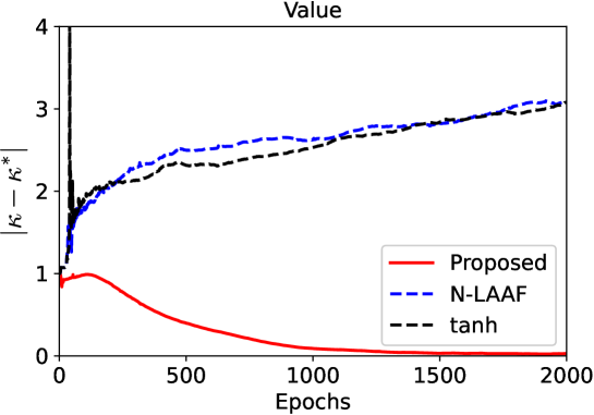
Figure 11: Convergence of $\left|\kappa-\kappa^{*}\right|$ of the Transient 1D Heat Transfer equation.

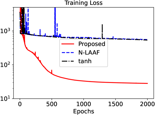
(a) Empirical convergence of training loss

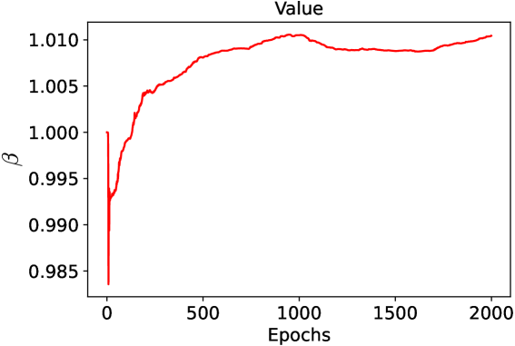
(b) Empirical convergence of $\beta^{i}_{k}$ in one of the neurons

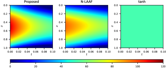
(c) Neural network solutions of the proposed method, N-LAAF, and tanh

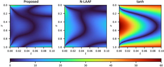
(d) Absolute difference maps for neural network solutions of the proposed method, N-LAAF, and tanh when compared to the approximate closed form solution

Figure 12: Results of the Transient 1D heat Transfer equation: (a) Empirical convergence of training loss; (b) Empirical convergence of $\beta^{i}_{k}$; (c) Neural network solutions of the proposed method, N-LAAF, and tanh; (d) Neural network solution of N-LAAF; (e) Absolute error maps for neural network solutions of the proposed method, N-LAAF, and tanh.

Figure 11 plots the convergence of absolute error $\left|\kappa-\kappa^{*}\right|$. Our method can converge to zero, which means that our approach can accurately identify the $\kappa^{*}$. Interestingly, the benchmark methods output a negative value of $\kappa$, which is physically meaningless, and they diverge away from the true $\kappa^{*}$ value. As a consequence of the absurd $\kappa$ values, the training losses of the benchmark methods hardly converge, whereas the proposed method reduces the loss function to lower orders of magnitude, as shown in Figure 12a. Figure 12b shows the convergence behavior of $\beta^{i}_{k}$ in one of the neurons. Figures 12c and 12d correspond to the neural network solutions and absolute error maps for different methods. Our method can obtain the most accurate solution, while the solution from PINN with N-LAAF is close to ours. The reason for poor performance of the tanh function in this case can be attributed to both the vanishing gradient and the higher order of magnitude of output values.

Table 2: Test performance of forward and inverse problems for different methods in terms of MSE and RE.

	tanh		N-LAAF		Proposed
	MSE	RE	MSE	RE	MSE	RE
Eq. (15)	295.10	0.8757	160.05	0.6449	0.00	0.0005
Eq. (17)	0.40	0.0088	0.21	0.0063	0.00	0.0000
Eq. (19)	2.61	0.7725	1.54	0.5936	0.55	0.3541
Eq. (20)	544.29	0.3927	564.08	0.3998	30.36	0.0928

The test performance for different methods in terms of MSE and RE is summarized in Table 2. The proposed method has the best performance in terms of MSE and RE. Based on the results in this Section, our proposed method can achieve the fastest training convergence and the best test performance for both forward and inverse problems using PINN.

5 Conclusion

In this work, a Self-scalable tanh (Stan) is proposed for PINN, which contains a trainable parameter. The trainable parameter can be easily optimized together with NN weights and biases using gradient descent algorithms. It is shown theoretically that the proposed Stan with PINN has no spurious stationary points, which is also empirically verified in all case studies. Our proposed Stan performs well on all types of case studies, including regression problems and a range of forward problems and an inverse problem. Especially, it is remarkably superior when the scales of the output are in higher orders of magnitude. Our proposed Stan can not only achieve faster convergence in training but also show better generalization in prediction, compared to state-of-the-art activation functions. In the inverse problem, it is shown to be significantly useful for identifying the thermal diffusivity with the simulated sensor data.

Though Stan improved the PINN to solve a wider range of problems, there are still some aspects of Stan that deserve further investigation. First, the theoretical properties of the Stan function should be examined, particularly related to the gradient flow in PINN. Second, the initialization of the trainable parameters $\beta^{i}_{k}$’s needs additional research. The $\beta^{i}_{k}$’s were initialized with constant values for all the neurons in this work. The third aspect which needs development is the optimization process, particularly for the characteristic of the proposed Stan activation function.

Appendix A Proof of Theorem 3

Proof.

The above statements can be proved by contradiction. For simplicity, fix $w_{\mathcal{F}}=w_{u}=1$. Suppose that the parameter vector $\tilde{\bm{\Theta}}=\{\bm{W}^{k},\bm{b}^{k}\}_{k=1}^{D}\bigcup\{\bm{\beta}^{k}\}_{k=1}^{D-1}$ is a limit point of $\{\tilde{\bm{\Theta}}_{m}\}_{m\geq 0}$ and a suboptimal stationary point.

Let $\ell_{f}^{j}\coloneqq\phi^{j}(u_{\tilde{\bm{\Theta}}}(\rho^{j}))$ and $\ell_{u}^{j}\coloneqq\left|u^{j}-u_{\tilde{\bm{\Theta}}}(\bm{x}_{u}^{j})\right|$. Denote $\bm{z}^{j,k}_{f}$ and $\bm{z}^{j,k}_{u}$ as the outputs of the $k$th layer for $\rho^{j}$ and $\bm{x}_{u}^{j}$, respectively. Now define

$$h_{f}^{i,j,k}\coloneqq\beta^{i}_{k}(\bm{W}^{k}_{i\cdot}\bm{z}^{j,k-1}_{f}+\bm{b}^{i,k})\in\mathbb{R}$$

and

$$h_{u}^{i,j,k}\coloneqq\beta^{i}_{k}(\bm{W}^{k}_{i\cdot}\bm{z}^{j,k-1}_{u}+\bm{b}^{i,k})\in\mathbb{R},$$

for all $i=1,\dots,N_{k}$, where $\bm{W}^{k}_{i\cdot}\in\mathbb{R}^{1\times N_{k}}$ denotes $i$th row in $\bm{W}^{k}$ and $\bm{b}^{i,k}\in\mathbb{R}$.

Based on the proofs in (Bertsekas,, 1997, Propositions 1.2.1-1.2.4), we have that $\nabla J_{\gamma}(\tilde{\bm{\Theta}})=\bm{0}$ and $J_{\gamma}(\tilde{\bm{\Theta}})<J_{\gamma}(\bm{0})$. Since $\nabla J_{\gamma}(\tilde{\bm{\Theta}})=\bm{0}$, for all $k=1,\dots,D$ and all $i=1,\dots,N_{k}$, we have

$$\frac{\partial J_{\gamma}(\tilde{\bm{\Theta}})}{\partial\bm{W}^{k}_{i\cdot}} =\frac{\beta_{i}^{k}}{N_{f}}\sum_{j=1}^{N_{f}}\frac{\partial\ell_{f}^{j}}{h_{f}^{i,j,k}}(\bm{z}^{j,k-1}_{f})^{\top}+\frac{\beta_{i}^{k}}{N_{u}}\sum_{j=1}^{N_{u}}\frac{\partial\ell_{u}^{j}}{h_{u}^{i,j,k}}(\bm{z}^{j,k-1}_{u})^{\top}=\bm{0}$$ (23)

$$\frac{\partial J_{\gamma}(\tilde{\bm{\Theta}})}{\partial\bm{b}^{i,k}} =\frac{\beta_{i}^{k}}{N_{f}}\sum_{j=1}^{N_{f}}\frac{\partial\ell_{f}^{j}}{h_{f}^{i,j,k}}+\frac{\beta_{i}^{k}}{N_{u}}\sum_{j=1}^{N_{u}}\frac{\partial\ell_{u}^{j}}{h_{u}^{i,j,k}}=0$$ (24)

In addition, for all $k=1,\dots,D-1$ and all $i=1,\dots,N_{k}$, we have

$$\frac{\partial J_{\gamma}(\tilde{\bm{\Theta}})}{\partial\beta^{i}_{k}} =\frac{1}{N_{f}}\sum_{j=1}^{N_{f}}\frac{\partial\ell_{f}^{j}}{h_{f}^{i,j,k}}(\bm{W}^{k}_{i\cdot}\bm{z}^{j,k-1}_{f}+\bm{b}^{i,k})+\frac{1}{N_{u}}\sum_{j=1}^{N_{u}}\frac{\partial\ell_{u}^{j}}{h_{u}^{i,j,k}}(\bm{W}^{k}_{i\cdot}\bm{z}^{j,k-1}_{u}+\bm{b}^{i,k})+2\gamma\beta^{i}_{k}$$ (25)

$$=0.$$

Multiply Eq. (25) by $\beta^{i}_{k}$, we have

$$0= \beta^{i}_{k}\frac{\partial J_{\gamma}(\tilde{\bm{\Theta}})}{\partial\beta^{i}_{k}}$$

$$= \frac{\beta^{i}_{k}}{N_{f}}\sum_{j=1}^{N_{f}}\frac{\partial\ell_{f}^{i}}{h_{f}^{i,j,k}}(\bm{W}^{k}_{i\cdot}\bm{z}^{j,k-1}_{f}+\bm{b}^{i,k})+\frac{\beta^{i}_{k}}{N_{u}}\sum_{j=1}^{N_{u}}\frac{\partial\ell_{f}^{u}}{h_{u}^{i,j,k}}(\bm{W}^{k}_{i\cdot}\bm{z}^{j,k-1}_{u}+\bm{b}^{i,k})+2\gamma(\beta^{i}_{k})^{2}$$

$$= \bm{W}^{k}_{i\cdot}(\frac{\partial J_{\gamma}(\tilde{\bm{\Theta}})}{\partial\bm{W}^{k}_{i\cdot}})^{\top}+\bm{b}^{i,k}\frac{\partial J_{\gamma}(\tilde{\bm{\Theta}})}{\partial\bm{b}^{i,k}}+2\gamma(\beta^{i}_{k})^{2}$$ (26)

$$= 2\gamma(\beta^{i}_{k})^{2},$$

where Eq. (26) comes from Eqs. (23) and (24). It implies that for all $\beta^{i}_{k}=0$ for all $i,k$ since $\gamma>0$. This shows $J_{\gamma}(\tilde{\bm{\Theta}})=J_{\gamma}(\bm{0})$, which contradicts with $J_{\gamma}(\tilde{\bm{\Theta}})<J_{\gamma}(\bm{0})$. ∎

References

- Baydin et al., (2018) Baydin, A. G., Pearlmutter, B. A., Radul, A. A., and Siskind, J. M. (2018). Automatic differentiation in machine learning: a survey. Journal of Marchine Learning Research, 18:1–43.
- Bertsekas, (1997) Bertsekas, D. P. (1997). Nonlinear programming. Journal of the Operational Research Society, 48(3):334–334.
- Bishop et al., (1995) Bishop, C. M. et al. (1995). Neural networks for pattern recognition. Oxford university press.
- Blechschmidt and Ernst, (2021) Blechschmidt, J. and Ernst, O. G. (2021). Three ways to solve partial differential equations with neural networks—a review. GAMM-Mitteilungen, 44(2):e202100006.
- Byrd et al., (1995) Byrd, R. H., Lu, P., Nocedal, J., and Zhu, C. (1995). A limited memory algorithm for bound constrained optimization. SIAM Journal on scientific computing, 16(5):1190–1208.
- Cai et al., (2021) Cai, S., Wang, Z., Wang, S., Perdikaris, P., and Karniadakis, G. E. (2021). Physics-informed neural networks for heat transfer problems. Journal of Heat Transfer, 143(6):0608011–15.
- Caudrey et al., (1975) Caudrey, P., Eilbeck, J., and Gibbon, J. (1975). The sine-gordon equation as a model classical field theory. Il Nuovo Cimento B (1971-1996), 25(2):497–512.
- Cengel, (2008) Cengel, Y. A. (2008). Introduction to thermodynamics and heat transfer: Engineering. McGraw-Hill.
- Crawford et al., (2018) Crawford, K. E., Ma, Y., Krishnan, S., Wei, C., Capua, D., Xue, Y., Xu, S., Xie, Z., Won, S. M., Tian, L., et al. (2018). Advanced approaches for quantitative characterization of thermal transport properties in soft materials using thin, conformable resistive sensors. Extreme Mechanics Letters, 22:27–35.
- Dodd et al., (1982) Dodd, R. K., Eilbeck, J. C., Gibbon, J. D., and Morris, H. C. (1982). Solitons and nonlinear wave equations. Academic Press, Inc.[Harcourt Brace Jovanovich, Publishers], London-New York ….
- Donea and Huerta, (2003) Donea, J. and Huerta, A. (2003). Finite element methods for flow problems. John Wiley & Sons.
- Goodfellow et al., (2016) Goodfellow, I., Bengio, Y., and Courville, A. (2016). Deep Learning. MIT Press. http://www.deeplearningbook.org.
- Gulcehre et al., (2016) Gulcehre, C., Moczulski, M., Denil, M., and Bengio, Y. (2016). Noisy activation functions. In International conference on machine learning, pages 3059–3068. PMLR.
- Harrsion et al., (2020) Harrsion, L., Ravan, M., Tandel, D., Zhang, K., Patel, T., and K Amineh, R. (2020). Material identification using a microwave sensor array and machine learning. Electronics, 9(2):288.
- Haykin and Lippmann, (1994) Haykin, S. and Lippmann, R. (1994). Neural networks, a comprehensive foundation. International journal of neural systems, 5(4):363–364.
- Hayou et al., (2019) Hayou, S., Doucet, A., and Rousseau, J. (2019). On the impact of the activation function on deep neural networks training. In International conference on machine learning, pages 2672–2680. PMLR.
- Hornik et al., (1989) Hornik, K., Stinchcombe, M., and White, H. (1989). Multilayer feedforward networks are universal approximators. Neural networks, 2(5):359–366.
- Jagtap and Karniadakis, (2020) Jagtap, A. D. and Karniadakis, G. E. (2020). Extended physics-informed neural networks (xpinns): A generalized space-time domain decomposition based deep learning framework for nonlinear partial differential equations. Communications in Computational Physics, 28(5):2002–2041.
- (19) Jagtap, A. D., Kawaguchi, K., and Em Karniadakis, G. (2020a). Locally adaptive activation functions with slope recovery for deep and physics-informed neural networks. Proceedings of the Royal Society A, 476(2239):20200334.
- (20) Jagtap, A. D., Kawaguchi, K., and Karniadakis, G. E. (2020b). Adaptive activation functions accelerate convergence in deep and physics-informed neural networks. Journal of Computational Physics, 404:109136.
- (21) Jagtap, A. D., Kharazmi, E., and Karniadakis, G. E. (2020c). Conservative physics-informed neural networks on discrete domains for conservation laws: Applications to forward and inverse problems. Computer Methods in Applied Mechanics and Engineering, 365:113028.
- Karniadakis et al., (2021) Karniadakis, G. E., Kevrekidis, I. G., Lu, L., Perdikaris, P., Wang, S., and Yang, L. (2021). Physics-informed machine learning. Nature Reviews Physics, 3(6):422–440.
- Kingma and Ba, (2014) Kingma, D. P. and Ba, J. (2014). Adam: A method for stochastic optimization. arXiv preprint arXiv:1412.6980, 22:1–43.
- Lagaris et al., (1998) Lagaris, I. E., Likas, A., and Fotiadis, D. I. (1998). Artificial neural networks for solving ordinary and partial differential equations. IEEE transactions on neural networks, 9(5):987–1000.
- LeCun et al., (2012) LeCun, Y. A., Bottou, L., Orr, G. B., and Müller, K.-R. (2012). Efficient backprop. In Neural networks: Tricks of the trade, pages 9–48. Springer.
- Leshno et al., (1993) Leshno, M., Lin, V. Y., Pinkus, A., and Schocken, S. (1993). Multilayer feedforward networks with a nonpolynomial activation function can approximate any function. Neural networks, 6(6):861–867.
- Mao et al., (2020) Mao, Z., Jagtap, A. D., and Karniadakis, G. E. (2020). Physics-informed neural networks for high-speed flows. Computer Methods in Applied Mechanics and Engineering, 360:112789.
- Mathew et al., (2020) Mathew, A., Amudha, P., and Sivakumari, S. (2020). Deep learning techniques: an overview. In International Conference on Advanced machine learning technologies and applications, pages 599–608. Springer.
- McCulloch and Pitts, (1943) McCulloch, W. S. and Pitts, W. (1943). A logical calculus of the ideas immanent in nervous activity. The bulletin of mathematical biophysics, 5(4):115–133.
- Mishra and Molinaro, (2020) Mishra, S. and Molinaro, R. (2020). Estimates on the generalization error of physics informed neural networks (pinns) for approximating a class of inverse problems for pdes. arXiv preprint arXiv:2007.01138.
- Misra, (2019) Misra, D. (2019). Mish: A self regularized non-monotonic activation function. arXiv preprint arXiv:1908.08681, 360:1–20.
- Moseley et al., (2021) Moseley, B., Markham, A., and Nissen-Meyer, T. (2021). Finite basis physics-informed neural networks (fbpinns): a scalable domain decomposition approach for solving differential equations. arXiv preprint arXiv:2107.07871.
- Nabian and Meidani, (2020) Nabian, M. A. and Meidani, H. (2020). Physics-driven regularization of deep neural networks for enhanced engineering design and analysis. Journal of Computing and Information Science in Engineering, 20(1):011006.
- No et al., (2021) No, A., Yoon, T., Sehyun, K., and Ryu, E. K. (2021). Wgan with an infinitely wide generator has no spurious stationary points. In International Conference on Machine Learning, pages 8205–8215. PMLR.
- Raissi and Karniadakis, (2018) Raissi, M. and Karniadakis, G. E. (2018). Hidden physics models: Machine learning of nonlinear partial differential equations. Journal of Computational Physics, 357:125–141.
- Raissi et al., (2019) Raissi, M., Perdikaris, P., and Karniadakis, G. E. (2019). Physics-informed neural networks: A deep learning framework for solving forward and inverse problems involving nonlinear partial differential equations. Journal of Computational physics, 378:686–707.
- Ramachandran et al., (2017) Ramachandran, P., Zoph, B., and Le, Q. V. (2017). Searching for activation functions. arXiv preprint arXiv:1710.05941, 13:1–21.
- Ranjan, (2020) Ranjan, C. (2020). Understanding deep learning: Application in rare event prediction. Connaissance Publishing.
- Rosenblatt, (1958) Rosenblatt, F. (1958). The perceptron: a probabilistic model for information storage and organization in the brain. Psychological review, 65(6):386.
- Rudd, (2013) Rudd, K. (2013). Solving partial differential equations using artificial neural networks. PhD thesis, Duke University.
- Rudd and Ferrari, (2015) Rudd, K. and Ferrari, S. (2015). A constrained integration (cint) approach to solving partial differential equations using artificial neural networks. Neurocomputing, 155:277–285.
- Safran and Shamir, (2018) Safran, I. and Shamir, O. (2018). Spurious local minima are common in two-layer relu neural networks. In International conference on machine learning, pages 4433–4441. PMLR.
- Sahli Costabal et al., (2020) Sahli Costabal, F., Yang, Y., Perdikaris, P., Hurtado, D. E., and Kuhl, E. (2020). Physics-informed neural networks for cardiac activation mapping. Frontiers in Physics, 8:42.
- Singh et al., (2019) Singh, S. K., Yang, R., Behjat, A., Rai, R., Chowdhury, S., and Matei, I. (2019). Pi-lstm: Physics-infused long short-term memory network. In 2019 18th IEEE International Conference On Machine Learning And Applications (ICMLA), pages 34–41. IEEE.
- Wang et al., (2021) Wang, S., Teng, Y., and Perdikaris, P. (2021). Understanding and mitigating gradient flow pathologies in physics-informed neural networks. SIAM Journal on Scientific Computing, 43(5):A3055–A3081.
- Wang et al., (2022) Wang, S., Yu, X., and Perdikaris, P. (2022). When and why pinns fail to train: A neural tangent kernel perspective. Journal of Computational Physics, 449:110768.
- Zhang and Gu, (2021) Zhang, Z. and Gu, G. X. (2021). Physics-informed deep learning for digital materials. Theoretical and Applied Mechanics Letters, 11(1):100220.
- Zhu et al., (2021) Zhu, Q., Liu, Z., and Yan, J. (2021). Machine learning for metal additive manufacturing: Predicting temperature and melt pool fluid dynamics using physics-informed neural networks. Computational Mechanics, 67(2):619–635.
- Zobeiry and Humfeld, (2021) Zobeiry, N. and Humfeld, K. D. (2021). A physics-informed machine learning approach for solving heat transfer equation in advanced manufacturing and engineering applications. Engineering Applications of Artificial Intelligence, 101:104232.