Fast Aquatic Swimmer Optimization with Differentiable Projective Dynamics and Neural Network Hydrodynamic Models

Abstract

Aquatic locomotion is a classic fluid-structure interaction (FSI) problem of interest to biologists and engineers. Solving the fully coupled FSI equations for incompressible Navier-Stokes and finite elasticity is computationally expensive. Optimizing robotic swimmer design within such a system generally involves cumbersome, gradient-free procedures on top of the already costly simulation. To address this challenge we present a novel, fully differentiable hybrid approach to FSI that combines a 2D direct numerical simulation for the deformable solid structure of the swimmer and a physics-constrained neural network surrogate to capture hydrodynamic effects of the fluid. For the deformable solid simulation of the swimmer’s body, we use state-of-the-art techniques from the field of computer graphics to speed up the finite-element method (FEM). For the fluid simulation, we use a U-Net architecture trained with a physics-based loss function to predict the flow field at each time step. The pressure and velocity field outputs from the neural network are sampled around the boundary of our swimmer using an immersed boundary method (IBM) to compute its swimming motion accurately and efficiently. We demonstrate the computational efficiency and differentiability of our hybrid simulator on a 2D carangiform swimmer. Due to differentiability, the simulator can be used for computational design of controls for soft bodies immersed in fluids via direct gradient-based optimization.

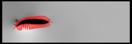
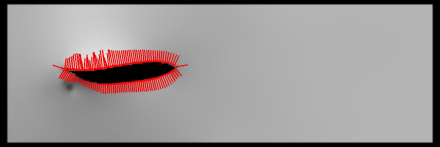
Figure 1: The forward swimming of a carangiform soft body fish immersed in fluid is simulated using our hybrid technique featuring FEM solid simulation and neural network based hydrodynamics. The figures illustrate at three separate time steps ($t$ = 73, 162, 275) both the fish and the full fluid pressure field. The red arrows at the interface from fluid to solid indicate the forces applied from the fluid to the fish. The forces are calculated with the immersed boundary method.

1 Introduction

Soft robotics is a rapidly advancing branch of robotics, showing promising results in non-standard settings in which compliant structures and bio-inspired designs are needed to solve tasks in natural environments (Hawkes et al., 2021). Aquatic locomotion is one such setting where soft robotic designs are uniquely able to take advantage of hydrodynamic properties, mimicking biological fish designs selected through evolutionary pressures for maximum fitness in nature (Katzschmann et al., 2018).

Simulation is a non-trivial challenge in the design of soft robots, as opposed to the rigid domain, for which established techniques have been developed and built upon in the span of decades. As for aquatic locomotion, solving fluid-structure interaction (FSI) for incompressible Navier-Stokes is a hard problem, traditionally extremely computationally expensive and thus often impossible in practice. Leveraging these simulations for design and control optimization generally involves an additional computational burden, through slow evolutionary or otherwise gradient-free optimization procedures. In this work, we leverage recent advances in machine learning for physics to take a step towards solving this problem, proposing a FSI simulation that is both orders of magnitude faster than standard approaches and fully differentiable, thus allowing for simple gradient-based optimization of design and control objectives.

To address the FSI challenge, our hybrid approach uses a differentiable numerical simulation for the deformable solid structure and a neural network surrogate to capture hydrodynamic effects of the fluid. To perform fast and differentiable soft body simulation of a flapping 2D carangiform swimmer, we leverage the finite-element method (FEM) combined with the novel approach of Differentiable Projective Dynamics (DiffPD) (Du et al., 2021b). For the fluid simulation, we train a physics-constrained neural network for hydrodynamics as proposed by Wandel et al. (2021a), which approximates fluidic flow on a discretized marker and cell (MAC) grid (Harlow & Welch, 1965). Their approach requires no training data but is instead trained using a physics-constrained loss based on the Navier-Stokes differential equation.

1.1 Our Contribution

Our contributions are the following:

• We introduce a differentiable layer linking the solid and the fluid simulations, achieving FSI coupling while maintaining low computational cost and full automatic differentiability. This approach involves the specification of the fluid boundary condition as a soft mask with techniques from differentiable rendering (Liu et al., 2019), and the computation of fluid-to-solid surface forces using a variation of the Immersed Boundary Method (IBM) (Peskin, 2002) with Gaussian distance.

• We demonstrate on a 2D carangiform swimmer that our hybrid approach leads to realistic swimming behavior with forward propulsion, while requiring considerably less computational resources than existing FSI simulations (Figure 1).

• We leverage the differentiability of the simulation to directly optimize the frequency parameter of a swimming controller with first order gradient optimization to achieve higher forward swimming speeds.

• We compare our hybrid simulation with the traditional COMSOL solver for FSI, demonstrating a monotonic relationship between the distance travelled by the fish with the same controller on either simulation.

2 Related Work

2.1 Soft Robotics and Aquatic Locomotion

To date there exist several examples of successful applications of soft robots in aquatic environments. Bio-inspired artificial fish robots (Katzschmann et al., 2016; Lin et al., 2021) mimicking biological fish have been deployed for a range of practical tasks, from exploration of underwater environments and observation of aquatic life (Katzschmann et al., 2018; Li et al., 2021) to protection of marine habitats against invasive species (Polverino et al., 2022).

Interest in the topic of aquatic locomotion has not been limited to robotics: the problem of learning swimming controls in simulation has received considerable attention from a reinforcement learning perspective (Gazzola et al., 2016; Colabrese et al., 2017; Verma et al., 2018), albeit relying on simple swimmer models that avoid the issues presented by soft bodies and FSI. For this reason, translating learnt controllers from these simulated works back to real-world robotics platforms (sim2real) remains an open challenge. Other works on aquatic locomotion simulation (Liu et al., 2015) do not involve learning controls altogether, but are limited to investigations into properties of biological swimmers through simulation.

2.2 Neural Networks for Hydrodynamics

Seminal work on Physics-Informed Neural Networks (PINNs) (Raissi et al., 2019) laid the foundations for the application of machine learning models as surrogate differential equations solvers. PINN training leverages the autodifferentiation properties of neural networks to learn the dynamics of differential equation systems without the need for costly training data, but using differential equation residuals directly as the model’s loss function.

A trove of subsequent works build on top of the PINN approach, refining the technique specifically for hydrodynamics problems (Mao et al., 2020; Raissi et al., 2020; Sun et al., 2020). Wandel et al. (2021a) propose a neural network model for hydrodynamics based on a discretized MAC grid and trained with a Navier-Stokes residual loss. While technically not following the original PINN specification, as the derivative terms in the Navier-Stokes loss are computed with finite differences on the grid as opposed to using autodifferentiation of the model inputs, their model allows for dynamic interactive specification of boundary conditions. For this reason, we adopt their model as a core component of our hybrid simulator. Further work from the same authors generalizes the technique to 3D simulations (Wandel et al., 2021b) and to higher turbulence fluids (Wandel et al., 2021c).

2.3 Differentiable Soft-Body Simulation

Differentiable soft-body simulation extends standard soft-body simulators to compute gradients for a soft body’s shape, control, or state parameters. Such gradients have been proven helpful in several downstream soft robotic applications, including system identification (Hu et al., 2019), trajectory optimization (Geilinger et al., 2020), motion control (Qiao et al., 2021), and shape optimization (Ma et al., 2021).

Mainstream differentiable soft-body simulators fall into two categories: physics-based and learning-based. Physics-based differentiable soft-body simulators derive gradients based on governing equations characterizing system dynamics and require domain-specific knowledge (Hu et al., 2019; Geilinger et al., 2020; Hu et al., 2020; Du et al., 2021b; Qiao et al., 2021). On the other hand, learning-based approaches aim to learn a neural network model approximating soft-body dynamics (Li et al., 2019; Pfaff et al., 2021). Such neural networks are naturally differentiable but, unlike their physics-based counterparts, typically lack guarantees on physics invariants, e.g., energy or momentum conservation. Additionally, their generalizability to new settings largely depends on the quality of the training data.

In this work, we use DiffPD (Du et al., 2021b), a recently developed physics-based differentiable soft-body simulator, to simulate our aquatic swimmers. While our algorithm is agnostic to the choice of differentiable simulators, we have found DiffPD beneficial because of its faster speed compared to other physics-based differentiable soft-body simulators and its extension to underwater robotics applications (Ma et al., 2021; Du et al., 2021a).

2.4 Fluid-Structure Interactions

Fluid-structure interaction (FSI) studies the complex behavior of fluids coupled with solid objects in a multi-physics system. FSI has been an extensively studied research topic in mechanical engineering, computational physics, and other related fields for many years (Dowell & Hall, 2001). Existing works on FSI typically focus on coupling fluids and rigid or soft objects under small deformations (Mucha et al., 2004; Zhang et al., 2007; Kalitzin & Iaccarino, 2003; Yang & Balaras, 2006). Numerical techniques for coupling fluids and nonlinear soft objects with large deformation have also been developed in computational physics and computer graphics (Feng et al., 2019; Brandt et al., 2019; Robinson-Mosher et al., 2008; Lu et al., 2016; Teng et al., 2016; Fang et al., 2020). Existing methods for FSI have been used to investigate the swimming behavior of fish (Curatolo & Teresi, 2015). These techniques provide accurate yet expensive computational tools for applications such as underwater soft swimmers covered in this work.

None of the FSI methods described above take into account gradient computation. Because of the already complicated coupling between fluids and solids, works on differentiable FSI are unsurprisingly sparse. Existing differentiable FSI approaches typically rely on non-physical simplifications of fluid, solid, or coupling models, e.g., assuming simple empirical fluid models (Ma et al., 2021; Du et al., 2021a) or limiting interactions to be local (Li et al., 2019; Pfaff et al., 2021). Compared with those previous works, our work is different because we attempt to incorporate the full physics in all possible aspects: Navier-Stokes equations for modeling fluids, continuum mechanics for modeling soft bodies, and immersed boundary methods (Peskin, 2002) (IBM), a representative FSI method, for modeling solid-fluid coupling.

3 Differentiable FSI Method

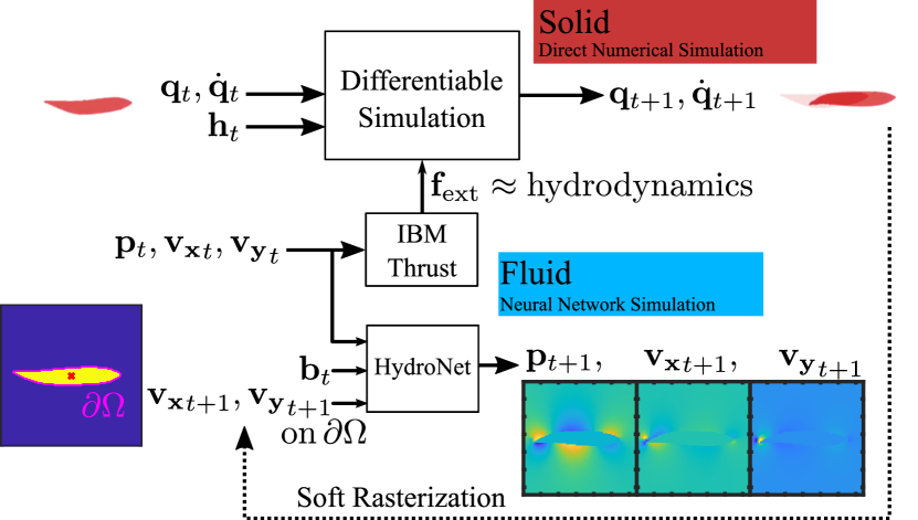
Figure 2: Overview block diagram of our hybrid simulation method. ${\bm{q}}$, $\dot{{\bm{q}}}$ are positions and velocities of finite elements; ${\bm{h}}$ are actuator signals; ${\bm{p}}$, ${\bm{v}}_{x}$ and ${\bm{v}}_{y}$ are pressure and velocity fields of the fluid; ${\bm{b}}$ is the soft boundary mask; $\mathbf{f}_{\mathrm{ext}}$ is the hydrodynamic force applied by the fluid to the solid.

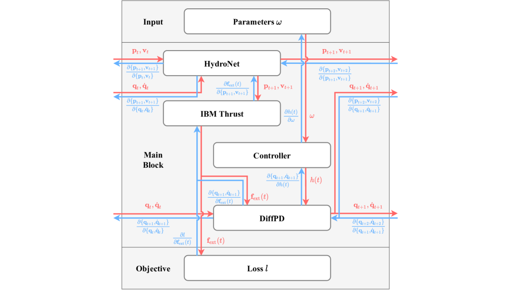
Figure 8: Detailed computation graph for our simulator. Red arrows represent forward pass computation, while blue arrows represent backward pass computation of gradients of the block’s variable with respect to forward pass quantitites.

We hereby detail our hybrid method for fast and fully differentiable simulation of soft body and fluid interaction. As shown in Figure 2, our approach consists of repeated, stacked interaction between the DiffPD solid simulator and the Hydrodynamics Neural Network (HydroNet) surrogate simulator. The output of the fluid simulation at time $t$ is used as input for the solid simulation at the same time $t$ through the introduction of an external fluidic force, while the output of the solid simulation at time $t$ is used as input for the fluid simulation at the next time step $t+1$ through the specification of a boundary condition. This interleaved interaction leads to the unfolding of a differentiable computation graph that can be backtraced by autodifferentiation frameworks to compute gradients through the entire simulation episode and optimize objectives (Figure 8). FEM element positions and velocities, actuations, fluid curls and pressures, boundary conditions, external forces and Young’s moduli are all differentiable with respect to each other. In the following sections, we describe each component of the system in detail.

3.1 Hydrodynamic Surrogate Simulation

Our goal for fluid simulation is that of obtaining a fast and differentiable surrogate model of hydrodynamics, so that swimmer designs and controls can be optimized by differentiating directly against the simulation environment, as opposed to doing so through evolutionary strategies or reinforcement learning.

In particular, our surrogate simulator needs to solve the incompressible Navier-Stokes equations describing fluidic flow costrained by Dirichlet boundary conditions. Given fluid density $\rho$ and viscosity $\mu$, and defining $\mathbf{v}$ and $\mathbf{p}$ to be velocity and pressure fields over a fluid domain $\Omega$, the equations consist of the following three terms:

$$\nabla\cdot\mathbf{v}=0 \qquad\text{on }\Omega\text{,}$$ (1)

$$\rho\left(\frac{\partial\mathbf{v}}{\partial t}+(\mathbf{v}\cdot\nabla)\mathbf{v}\right)=-\nabla\mathbf{p}+\mu\nabla^{2}\mathbf{v} \qquad\text{on }\Omega\text{,}$$ (2)

$$\mathbf{v}=\mathbf{v}_{d} \qquad\text{on }\partial\Omega\text{.}$$ (3)

Equation (1) is called the divergence term, and forces incompressibility of the fluid, disallowing any sources or sinks within $\Omega$. Equation (2) is the main hydrodynamic term, stating that changes in fluidic particle momentum must correspond to forces exerted by the pressure gradient and viscous friction. Equation (3) is the Dirichlet boundary condition, stating that velocities on the boundary $\partial\Omega$ of the fluidic domain must be equal to the supplied boundary velocities $\mathbf{v}_{d}$.

The equations can be simplified for the 2D case by observing that the Helmholtz theorem allows to decompose the velocities into a curl free part and a divergence-free part

$$\mathbf{v}=\nabla\mathbf{q}+\nabla\times\mathbf{a}\text{.}$$ (4)

By expressing velocities as $\mathbf{v}=\nabla\times\mathbf{a}$, with the curl $\mathbf{a}$ being one-dimensional in the 2D case, we implicitly force zero-divergence in our fluid without the need for explicitly solving for Equation (1).

To solve the equations, we train an unsupervised neural network model following the approach proposed by Wandel et al. (2021a). The model in focus is a U-net (Ronneberger et al., 2015) with limited convolutional channels that operates on discretized fields on a marker and cell (MAC) (Harlow & Welch, 1965) grid. The model takes as input the curl field $\mathbf{a}$, the pressure field $\mathbf{p}$, the boundary mask $\mathbf{b}$ identifying the domain $\Omega$, and the boundary velocities $\mathbf{v}_{d}$ from time step $t$. The model predicts as output the curl field $\mathbf{a}$ and the pressure field $\mathbf{p}$ for the next time step $t+1$, given a constant time step magnitude $h$.

The model is not trained on simulation data, but instead uses the Navier-Stokes residuals as its loss function:

$$L_{p} =\left\|\rho\left(\frac{\partial\mathbf{v}}{\partial t}+(\mathbf{v}\cdot\nabla)\mathbf{v}\right)+\nabla\mathbf{p}-\mu\nabla^{2}\mathbf{v}\right\|^{2}\quad\text{on }\Omega\text{,}$$ (5)

$$L_{b} =\left\|\mathbf{v}-\mathbf{v}_{d}\right\|^{2}\quad\text{on }\partial\Omega\text{,}$$ (6)

$$L =\beta L_{p}+\gamma L_{b}\text{.}$$ (7)

with parameters $\beta$ and $\gamma$ determining how much to prioritize the Navier-Stokes term or the boundary term.

Given this loss, the network is trained on synthetic episodes consisting of randomly generated boundary conditions, with the network’s curl and pressure fields output being fed back as training data at each iteration. This way, the physics-constrained loss is applied to increasingly realistic scenarios.

3.2 Differentiable Soft-Body Simulation

We model the soft-body dynamics by the following governing equations from continuum mechanics (Sifakis & Barbic, 2012):

$$\rho_{s}\ddot{{\bm{q}}}=\nabla\cdot\mathbf{P}+\mathbf{f}_{\textrm{ext}},$$ (8)

where $\rho_{s}$ stands for the soft material’s density, ${\bm{q}}={\bm{q}}(\mathbf{X},t)$ tracks the position of a material point $\mathbf{X}$ from the material space (undeformed shape) at time $t$, $\mathbf{P}$ represents the first Piola-Kirchoff stress tensor, and $\mathbf{f}_{\text{ext}}$ captures all external forces applied to $\mathbf{X}$ at time $t$. We refer interested readers to Sifakis & Barbic (2012) for more background information regarding soft-body simulation. The stress $\mathbf{P}$ determines the behavior of soft material and is specified by choosing soft material models. In this work, we use the linear co-rotated material model as suggested by DiffPD because of its balance between speed (Bouaziz et al., 2014) and physical accuracy (Du et al., 2021a; Zhang et al., 2021).

Given the continuous equations above, DiffPD uses standard finite-element methods (FEM) and the implicit time-stepping scheme to discretize the dynamic system spatially and temporally, leading to the nonlinear system of equations below:

$${\bm{q}}_{t+1} ={\bm{q}}_{t}+h\dot{{\bm{q}}}_{t+1},$$ (9)

$$\dot{{\bm{q}}}_{t+1} =\dot{{\bm{q}}}_{t}+h\rho_{s}^{-1}(\mathbf{f}_{\textrm{ext}}+\mathbf{f}_{\textrm{int}}(\mathbf{x}_{t+1})),$$ (10)

where ${\bm{q}}$ and $\dot{{\bm{q}}}$ now represent nodal positions and velocities of finite elements at time steps specified by their subscripts. The notation $\mathbf{f}_{\text{int}}$ denotes the elastic force induced by the stress tensor $\mathbf{P}$. Once the forward simulation process is established, DiffPD derives its gradients using standard chain rules and adjoint methods. Interested readers can refer to DiffPD (Du et al., 2021b) for detailed derivations of these equations.

3.3 Differentiable Fluid-Structure Interaction

FSI involves solving a two-way link between the DiffPD soft structure FEM simulation and our neural network hydrodynamic surrogate simulation. Hydrodynamic forces from the fluid simulation affect the soft body finite elements as an external force $\mathbf{f}_{\textrm{ext}}$, at the same time the soft body simulation determines the Dirichlet boundary conditions $\mathbf{b}$ and $\mathbf{v}_{d}$ for the hydrodynamics simulation. An additional cause of complexity stems from the fact that these operations must mediate between a Lagrangian and a discrete Eulerian representation for physical quantities, with the former being used the the solid simulation, and the latter for the fluid simulation.

Lagrangian methods handle physics simulation by modeling individual particles constituting the simulated material. DiffPD operates in a Lagrangian fashion, as the finite elements identified by ${\bm{q}}$ and $\dot{{\bm{q}}}$ track specific points within the soft body and move along with the body within the domain. Opposed to this, discrete Eulerian methods simulate PDEs on a discretized grid such as the fixed MAC grid used by Wandel et al. (2021a)’s hydrodynamics network. With this representation, $\mathbf{v}$ and $\mathbf{p}$ summarise fluid properties on fixed locations of the domain, without tracking individual fluid particles.

The challenge in this setting is that of providing a differentiable layer to compute these interaction quantities which mediate between representations. For the solid-to-fluid interaction, the Lagrangian elements described by ${\bm{q}}$ and $\dot{{\bm{q}}}$ must be used to compute a boundary mask $\mathbf{b}$ with a rasterization operation, which is however generally non-differentiable. Similarly, grid boundary velocities $\mathbf{v}_{d}$ are generally computed with a non-differentiable neighbourhood averaging operation. For the fluid-to-solid interaction, we turn to the fluid-to-solid stage of the Immersed Boundary Method (IBM) (Peskin, 2002), which samples Eulerian pressure values $\mathbf{p}$ on locations near the boundary in order to compute Lagrangian external forces $\mathbf{f}_{\textrm{ext}}$ affecting the solid finite elements.

Solid-to-Fluid Coupling

Given the state of the DiffPD soft body simulation from a specific time step, the finite element positions ${\bm{q}}$ and velocities $\dot{{\bm{q}}}$ fully determine the boundary condition for the subsequent hydrodynamic simulation step. The positions ${\bm{q}}$ determine the shape and location of the fish body, served as input to the Hydronet as a boundary mask $\mathbf{b}$. The velocities $\dot{{\bm{q}}}$ are instead used to compute the boundary velocities $\mathbf{v}_{d}$ as a granular cell-wise velocity obtained by averaging the closest elements to each boundary cell.

There is however a non trivial obstacle that renders a naive application of the boundary mask from Wandel et al. (2021a) non applicable to our optimization setting. By definition, the rasterization operation computing a binary mask is non-differentiable, thereby breaking the chain of differentiability which we rely on for optimization.

Our solution to this issue takes from the field of differentiable rendering (Liu et al., 2019), and in particular to the techniques associated with soft rasterization. Instead of producing a hard binary mask as a rasterization of the robot’s finite element mesh, we use a signed distance field to produce a soft differentiable mask, with real-valued entries $\mathbf{b}_{ij}\in[0,1]$.

Define ${\bm{x}}_{ij}\in\mathbb{R}^{2}$ as the spatial coordinates of the MAC grid cell in position $(i,j)$ and ${\bm{q}}^{k}$ those of the $k$-th finite element. Then each cell ${\bm{b}}_{ij}$ from the soft boundary mask is computed as

$$\mathbf{b}_{ij}=\text{sigm.}\left(\delta_{ij}\frac{\sum_{l}\left(\text{softmin}_{k}\frac{\|{\bm{x}}_{ij}-{\bm{q}}^{k}\|^{2}}{\xi}\right)_{l}\|{\bm{x}}_{ij}-{\bm{q}}^{l}\|^{2}}{\sigma}\right)$$ (11)

with $\sigma$ and $\xi$ being mask softness parameters, $\|\cdot\|^{2}$ the Euclidean distance and $\delta_{ij}=+1$ if the cell location ${\bm{x}}_{ij}$ is inside the fish body, while $\delta_{ij}=-1$ if outside.

We can similarly use a differentiable surrogate to obtain cell-wise fine-grained boundary velocities:

$${{\bm{v}}_{d}}_{ij}=\left(\sum_{l}{\left(\text{softmin}_{k}\frac{\|{\bm{x}}_{ij}-{\bm{q}}^{k}\|^{2}}{\tau}\right)_{l}{\dot{{\bm{q}}}}^{l}}\right)\cdot{\bm{b}}_{ij}$$ (12)

with $\tau$ being a softness parameter.

Tuning the softness parameters $\sigma$, $\xi$ and $\tau$ allows us to tune the trade-off between boundary accuracy and smooth gradients.

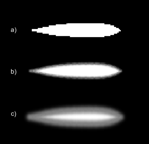
Figure 3: Soft boundary masks obtained with the softness parameters $\xi=$ 5e-7 and a) $\sigma=$ 5e-9, b) $\sigma=$ 5e-7, c) $\sigma=$ 5e-5.

Fluid-to-solid coupling

The overall purpose of our hybrid simulation approach is to optimize fish designs and/or control policies with respect to a more realistic model of hydrodynamics. Therefore, the mechanism by which the hydrodynamics simulation affects the soft body simulation is of utmost importance.

The way for hydrodynamic forces to affect DiffPD is through an external force $\mathbf{f}_{\textrm{ext}}$ applied to the simulation’s finite elements. Common drag/thrust optimizations such as that of Chen et al. (2021) often average the force over the entire solid surface. This force is shaped by two contributions, one due to the pressure field,

$$\mathbf{f}_{\textrm{pressure}}=-\int_{\partial\Omega}\mathbf{p}\cdot\mathbf{n}\,dl,$$ (13)

and the other is due to the velocity field,

$$\mathbf{f}_{\textrm{viscous}}=-\int_{\partial\Omega}\mu\mathbf{n}\times\mathbf{a}\,dl\text{,}\quad\mathbf{a}=\nabla\times\mathbf{v},$$ (14)

with $\partial\Omega$ being the solid body boundary and $\mathbf{n}$ its outward pointing normal vector. Total hydrodynamic force is obtained by summing $\mathbf{f}_{\textrm{ext}}=\mathbf{f}_{\textrm{pressure}}+\mathbf{f}_{\textrm{viscous}}$. However, for common water-like fluids with low viscosity $\mu$, the contribution of the viscous term $\mathbf{f}_{\textrm{viscous}}$ can be considered negligible and its computation can be omitted.

Figure 4: Our immersed boundary method for fluid-to-solid interaction. Each soft body surface element (red) is subjected to an external force ${\mathbf{f}_{\mathrm{ext}}}_{k}$ in the opposite direction of its normal $\mathbf{n}_{k}$. To compute the scalar force magnitude, nearby Eulerian cells from the pressure field are averaged with a Gaussian function centered around the element.

Given that our approach for solid simulation is based on finite elements, with each surface element $k$ being associated with its surface normal ${\bm{n}}_{k}$, we can compute individual elements’ surface forces ${\mathbf{f}_{\textrm{ext}}}_{k}$. To bridge the Eulerian to Lagrangian gap, we adopt the IBM fluid-to-solid step on forces

$${\mathbf{f}_{\textrm{ext}}}_{k}=-l_{k}{\bm{n}}_{k}\sum_{i,j}{{\bm{p}}_{ij}\delta\left(\mathbf{x}_{ij}-{\bm{q}}^{k}\right){\bm{b}}_{ij}}$$ (15)

where $\delta$ is the Dirac delta and $l_{k}=(\|{\bm{q}}^{k-1}-{\bm{q}}^{k}\|+\|{\bm{q}}^{k}-{\bm{q}}^{k+1}\|)/2$ is the surface length corresponding to finite element $k$. With the IBM, we are able to appropriately identify the force applied to Lagrangian element $k$, despite only having access to pressures on a fixed Eulerian grid.

In practice, due to the finite discretization, it is not feasible to adopt $\delta$ directly, but a surrogate $\tilde{\delta}({\bm{x}})=\phi(x_{1})\phi(x_{2})$ must be chosen such that it satisfies several properties as detailed in the original IBM paper (Peskin, 2002):

$$\phi(r)\text{ is continuous for all real }r\text{,}$$ (16)

$$\sum_{j<r}\phi(r-j)=\sum_{j>r}\phi(r-j)=\frac{1}{2}\text{ for all real }r\text{,}$$ (17)

$$\sum_{j}(r-j)\phi(r-j)=0\text{ for all real }r\text{,}$$ (18)

$$\sum_{j}(\phi(r-j))^{2}=C\text{ for all real }r\text{,}$$ (19)

where the constant $C$ is independent of $r$. The original formulation from Peskin (2002) included the additional property of $\phi(r)=0$ for $|r|>2$, however this is not strictly required and is only introduced for computational cost reasons, which are moot if the operation is performed with GPU parallelism.

We thus choose to use a normalized Gaussian distance for our IBM, namely in the form

$$\tilde{\delta}({\bm{x}}-{\bm{y}})=\exp\left(-\frac{\|{\bm{x}}-{\bm{y}}\|^{2}}{2\sigma^{\prime}}\right)\text{,}$$ (20)

with $\sigma^{\prime}$ being a smoothness parameter and the equation satisfying all relevant properties.

This choice then leads to our IBM formula for calculating individual elements’ ${\mathbf{f}_{\textrm{ext}}}_{k}$:

$${\mathbf{f}_{\textrm{ext}}}_{k}=-l_{k}{\bm{n}}_{k}\sum_{i,j}{{\bm{p}}_{ij}\frac{1}{Z}\exp\left(-\frac{\|\mathbf{x}_{ij}-{\bm{q}}^{k}\|^{2}}{2\sigma^{\prime}}\right){\bm{b}}_{ij}}\text{,}$$ (21)

with $Z=\sum_{i,j}\exp\left(-\frac{\|\mathbf{x}_{ij}-{\bm{q}}^{k}\|^{2}}{2\sigma^{\prime}}\right){\bm{b}}_{ij}$ being a normalization constant.

The reason we choose a Gaussian delta function is not only because of the increased stability due to larger function support (as is discussed by Peskin (2002)). Using a Gaussian as opposed to the original Dirac delta gives us the property of differentiability of the forces with respect to the entire pressure field. Once again, there is a trade-off between gradient smoothness and IBM precision, as lower $\sigma^{\prime}$ allows for more precise IBM interpolation, but causes the gradients with respect to the pressure field to vanish for most locations.

The obtained $\mathbf{f}_{\mathrm{ext}}$ is at the granularity of individual finite elements. It can either be applied as a DiffPD input as-is, allowing for precise but potentially unstable simulation of surface interaction, or it can be used to compute the overall thrust/drag

$$\mathbf{f}_{\textrm{ext}}=\sum_{k}{\mathbf{f}_{\textrm{ext}}}_{k}$$ (22)

which, divided by the total finite element number, can be applied as an average force to all the solid finite elements, to only model directional thrust.

3.4 Limitations

Our FSI simulator is fast and differentiable, and its hydrodynamics component is trainable on several different fluid parameter settings, also supporting both still and moving flow scenarios for swimmers (through setting of the inflow velocity as a boundary condition). However, this does not mean that the method is without limitations. For instance, the method does not generalize to flow velocities well outside those imposed by inflow boundary conditions during HydroNet training. The simulation can also present instabilities if the forces involved are too strong or applied suddenly between frames: for this reason we explictly set a burn-in number $N_{\text{burn-in}}$ of iterations during which surface forces $\mathbf{f}_{\textrm{ext}}$ are linearly smoothed by a factor of $t/N_{\text{burn-in}}$.

4 Experimental Setup and Results

4.1 Soft Carangiform Swimmer

Our main experimental setting is controller optimization for a soft body carangiform swimmer immersed in Navier-Stokes fluid with parameters resulting in various degrees of turbulence.

The swimmer’s profile is generated using a parametric polynomial $c(X)$ adapted from Curatolo & Teresi (2015) and the actuation envelope is obtained with a parametric curve adapted from Videler & Hess (1984) as shown in Figure 5. This parametric shape is discretized as a mesh, which is used to define the finite elements for DiffPD. We set the fish body’s Youngs’ modulus as $E=$6\text{\times}{10}^{5}\text{\,}\mathrm{Pa}$$, its Poisson ratio as $\nu=0.45$ and its density as $\rho_{s}=$100\text{\,}\mathrm{k}\mathrm{g}\mathrm{/}\mathrm{m}^{3}$$. We refer to Appendix B for further details.

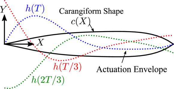
Figure 5: Coordinate system of the fish in the material frame, where $c(X)$ is the parametric shape of the carangiform fish and $h(X,t)$ is the actuation envelope (defined in Appendix B).

4.2 HydroNet Training

We model our fluid medium as a quadrilateral 2D box of size $$0.25\text{\,}\mathrm{m}$\times$0.75\text{\,}\mathrm{m}$$, discretized as a $100\times 300$ MAC grid with resolution of $2.5\text{\,}\mathrm{mm}$, and computed with time step $h=$0.01\text{\,}\mathrm{s}$$.

To immerse the solid simulation in a suitable water-like environment at this scale, we retrain the hydrodynamics network from Wandel et al. (2021a), performing a hyperparameter search on model hyperparameters and loss scalings to train for density $\rho\in[$10\text{\,}\mathrm{k}\mathrm{g}\mathrm{/}\mathrm{m}^{3}$,$50\text{\,}\mathrm{k}\mathrm{g}\mathrm{/}\mathrm{m}^{3}$]$ and viscosity $\mu\in[$0.125\text{\,}\mathrm{m}\mathrm{Pa}\cdot\mathrm{s}$,$1\text{\,}\mathrm{m}\mathrm{Pa}\cdot\mathrm{s}$]$. The resulting hydrodynamic networks model a variety of fluid environments, from conditions close to laminar flow to turbulent, light-water scenarios.

The main tuning challenge for training the network on the desired fluid parameters is that of re-scaling the terms appearing in the losses (Equations (5) and (6)), which in Wandel et al. (2021a) operate on time and space resolutions of whole seconds and metres. Given that we require a much finer resolution, re-scaling the equation terms by a factor of $1/0.0025=400$ allowed the training to converge.

4.3 FEM Validation with COMSOL

Our hybrid simulator has the properties of being fast and differentiable. However, the HydroNet component of our simulator makes it fundamentally a surrogate model with no strict numerical guarantees. It is therefore apparent that while using such a hybrid simulator model for design and control optimization will result in much faster convergence towards a solution, it will not evaluate such solution with respect to the underlying physical ground truth.

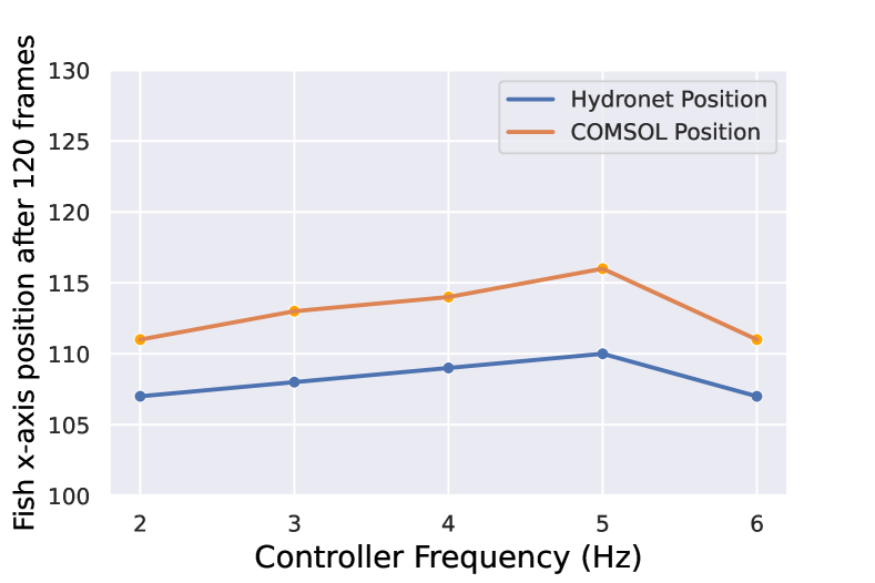
Figure 6: Comparison of travelled distance on the x-axis between COMSOL Multiphysics and our HydroNet simulator.

We therefore propose to benchmark our simulator against COMSOL Multiphysics for the forward swimming carangiform task, using FEM numerical simulation to model both hydrodynamics, soft body physics, and FSI (see Appendix C for further details). Our comparison of a surrogate model against a slow, non-differentiable, but physically-validated simulation is akin to performing sim2real validation (more appropriately, sim2sim). For a further baseline, we attempted a comparison with a heuristic hydrodynamic formula from the work of Min et al. (2019) commonly used in applications, however, this produced overly non-physical results, resulting in wholly incomparable motion.

Due to inherent chaotic behavior of the hydrodynamic system, it is impossible to perform direct step-by-step comparisons between simulation quantities, as any small difference can cause explicit residuals between the simulations to diverge. We therefore instead compare overall fish traveled distance between the simulations for different frequency parameter values of the controller: if the simulations maintain monotonicity of performance as a function of the parameter, then optimizing the parameter on the surrogate simulation will achieve high performance on the costly, realistic simulation. This is in contrast to Min et al. (2019)’s baseline, which results in off-scale, incomparable motion and thus would offer no guarantees on physical optimality.

Table 1: Runtime comparison between our hybrid simulator and COMSOL Multiphysics for a 300 frame episode. Note that COMSOL Multiphysics does not produce gradients and a fair comparison is therefore only to be made between COMSOL Multiphysics’s total runtime and our simulator’s forward pass. Also note that due to gradient checkpointing, the backward pass for our approach is slower than theoretically achievable.

Hybrid sim (ours)	Time
HydroNet Warmup	$$44\text{\,}\mathrm{s}$\pm$0.2\text{\,}\mathrm{s}$$
Total Forward pass	$3\text{\,}\mathrm{min}$ $$33\text{\,}\mathrm{s}$\pm$16.8\text{\,}\mathrm{s}$$
Forward pass: DiffPD	$2\text{\,}\mathrm{min}$ $$50\text{\,}\mathrm{s}$\pm$16.5\text{\,}\mathrm{s}$$
Forward pass: Hydronet	$$43\text{\,}\mathrm{s}$\pm$0.3\text{\,}\mathrm{s}$$
Backward pass	$3\text{\,}\mathrm{min}$ $$57\text{\,}\mathrm{s}$\pm$17.9\text{\,}\mathrm{s}$$
COMSOL Multiphysics	Time
Total runtime	$5\text{\,}\mathrm{h}$ $16\text{\,}\mathrm{min}$ $39\text{\,}\mathrm{s}$

We compare our carangiform swimmer simulation against COMSOL Multiphysics, modeling the swimmer as described in Section 4.1 immersed in fluid with $\rho=$50\text{\,}\mathrm{k}\mathrm{g}\mathrm{/}\mathrm{m}^{3}$$ and $\mu=$0.125\text{\,}\mathrm{m}\mathrm{Pa}\cdot\mathrm{s}$$. Figure 6 illustrates the comparison in terms of x-axis location of the swimmer’s head at the end of an episode of 120 frames ($1.2\text{\,}\mathrm{s}$) for controllers with frequency between 3 and $7\text{\,}\mathrm{Hz}$. As apparent, despite the presence of a systematic mismatch of on average 6 grid-units (equal to $6\cdot$2.5\text{\,}\mathrm{mm}$$ = $15\text{\,}\mathrm{mm}$), both simulations behave monotonically with respect to optimality of the frequency parameter, achieving the same maximum of travelled distance at $5\text{\,}\mathrm{Hz}$. In Table 1, we compare runtimes for our simulator and COMSOL, observing a speedup in the order of 100x.

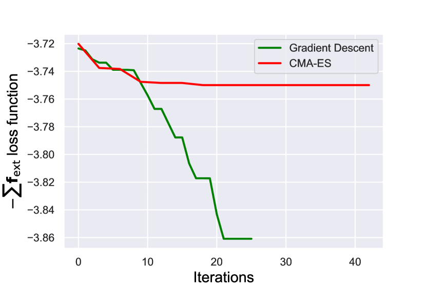
Figure 7: History plot of the controller frequency optimization, comparing gradient descent with the gradient-free CMA-ES method.

4.4 Controller Frequency Optimization

To demonstrate the typical use case for our fully differentiable hybrid simulator, we set up a forward swimming task for the carangiform swimmer with the controller as defined in Section 4.1, optimizing the total forward thrust $L_{\text{opt}}=-\sum_{t\in[1,T]}\mathbf{f}_{\mathrm{ext}}(t)_{x}$ for a simulation episode of length $T=500$ and time step $h=$0.01\text{\,}\mathrm{s}$$. Moreover, we fix the fish’s movement to be centered along the x axis, to favor modeling of forward speed only. The objective is to optimize the controller’s angular frequency $\omega$. We apply pressure thrust forces to the fish as an averaged vector $\mathbf{f}_{\mathrm{ext}}$ to limit drift and focus the optimization on swimming performance. To backpropagate over the long episode within memory limits, we resort to gradient checkpointing in between simulation steps.

The optimization experiment of the controller frequency was done in fluid medium with $\rho=$50\text{\,}\mathrm{k}\mathrm{g}\mathrm{/}\mathrm{m}^{3}$$ and $\mu=$0.125\text{\,}\mathrm{m}\mathrm{Pa}\cdot\mathrm{s}$$. The experiment was initialized with a frequency of $2\text{\,}\mathrm{Hz}$ and used Adam optimizer. As seen in Figure 7, the optimization converged after 21 iterations to a frequency of $6.3\text{\,}\mathrm{Hz}$. As benchmark comparison, the evolutionary strategy CMA-ES (Hansen, 2016), initialized with an uninformative standard deviation of $\sigma=1$, never leaves its initialization neighbourhood within the optimization budget, obtaining its best value at the frequency of $2.63\text{\,}\mathrm{Hz}$. The found optimum is different from that of Section 4.3 due to our fixing of the x axis, ignoring any sideways motion.

5 Conclusion

In this work, we introduced a fast, differentiable and accurate FSI simulation for immersed soft bodies. We demonstrated the suitability of our FSI simulation for simulating forward swimming motion of a carangiform swimmer, and we tested its use for the optimization of the frequency of a swimming controller. We believe our method paves the way for more complex but fast multi-physics simulations that couple fluid mechanics with continuum mechanics in a unified framework. An extension of our method has the potential to in the future enable ambitious works on physically accurate co-optimization of shape and control for many applications including vehicle design and soft robot optimization.

Appendix A Detailed Computation Graph

Appendix B Fish Parametric Actuation

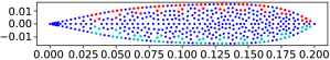
Figure 9: Discretized elements and actuated elements in the top half (red), and the bottom half (light blue) for the soft fish.

As shown in Figure 9, we specify spaced elements on the fish surface to be actuated by contraction, with each actuated element in longitudinal position $X$ receiving an actuation signal $h(X,t)$ at time $t$. The carangiform style of swimming can be described by the following $h(X,t)$ with a backward-traveling wave and envelope:

$$h(X,t)=Cv(X)\sin(\gamma X+\omega t)(1-e^{-\frac{t}{t_{a}}}),$$ (23)

where $C$ is a constant, $v(X)$ is the envelope of maximum lateral displacement, $\gamma$ the wave number of body undulations, $\omega$ the angular frequency, $c_{0}=\omega/\gamma$ the wave speed, and $t_{a}$ is the activation time. The envelope function $v(X)$ is given by

$$v(X)=\frac{4}{25L}X^{2}-\frac{6}{25}X+\frac{1}{10}L,$$ (24)

where $L$ is the length of the fish, which for our case is $L=$0.2\text{\,}\mathrm{m}$$.

Appendix C The COMSOL Material Model

The fish is modeled as an isotropic and linear elastic solid in COMSOL Multiphysics. The Piola-Kirchoff stress (or engineering stress) is

$$\mathbf{S}^{e}=2\mu_{s}\mathbf{E}^{e}+\lambda_{s}\textrm{tr}(\mathbf{E}^{e})\mathbf{I},$$ (25)

where $\mu_{s}$, $\lambda_{s}$ are the Lamé moduli and $\mathbf{E}^{e}$ is the Green-Lagrange strain. We can use an additive decomposition of the strain as

$$\mathbf{E}=\mathbf{E}^{e}+\mathbf{E}^{m},$$ (26)

where $\mathbf{E}^{m}=\mathbf{E}^{m}(X,Y,t)$ is a time-evolving distortion strain that models the actuation of muscles. The Green-Lagrange strain can be written in terms of the deformation gradient as

$$\mathbf{E}=\frac{1}{2}(\mathbf{F}^{\top}\mathbf{F}-\mathbf{I}).$$ (27)

The deformation gradient permits the multiplicative decomposition

$$\mathbf{F}=\mathbf{F}^{e}\mathbf{F}^{m}.$$ (28)

Note: by defining the elastic deformation as (26), the elastic deformation is

$$\mathbf{E}^{m}=\frac{1}{2}{\mathbf{F}^{m}}^{\top}({\mathbf{F}^{e}}^{\top}\mathbf{F}^{e}-\mathbf{I})\mathbf{F}^{m}.$$ (29)

To generate a flexural motion, we relate the distortion $\mathbf{E}^{m}$ to the curvature and the lateral displacement

$$E^{m}_{xx}(X,Y,t)=-Y\frac{\partial^{2}h(X,t)}{\partial X^{2}},$$ (30)

where $Y=h(X,t)$, with $h(X,t)$ being the actuation scheme described in Section 4.1, and the other components of $\mathbf{E}^{m}$ are identically zero.

Appendix D COMSOL Comparison plots

The following plots qualitatively illustrate our comparison between our approach and the COMSOL simulation.

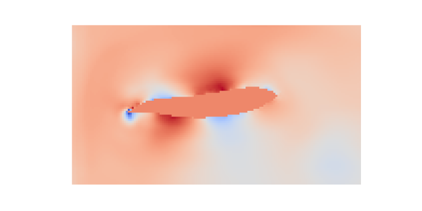
Figure 10: Ours: DiffPD + HydroNet swimmer simulation.

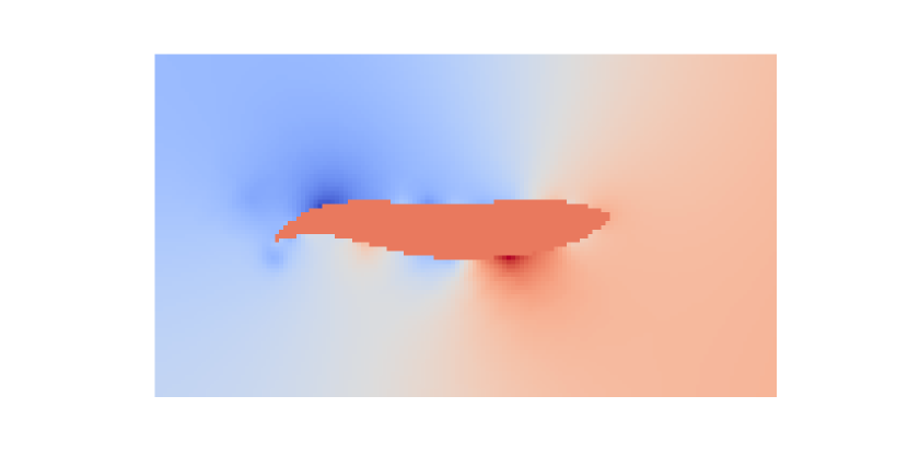
Figure 11: COMSOL swimmer simulation.

Figure 12: Normalized pressure fields for a frame of the two simulations.

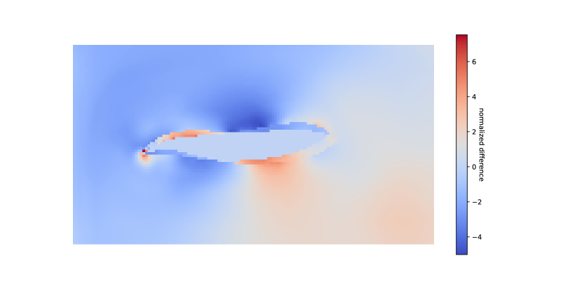
Figure 13: Overlay of the normalized pressure fields of our DiffPD + HydroNet simulation and the COMSOL simulation.

References

- Bouaziz et al. (2014) Bouaziz, S., Martin, S., Liu, T., Kavan, L., and Pauly, M. Projective dynamics: fusing constraint projections for fast simulation. ACM Transactions on Graphics, 33(4):154:1–154:11, July 2014. ISSN 0730-0301. doi: 10.1145/2601097.2601116. URL https://doi.org/10.1145/2601097.2601116.
- Brandt et al. (2019) Brandt, C., Scandolo, L., Eisemann, E., and Hildebrandt, K. The reduced immersed method for real-time fluid-elastic solid interaction and contact simulation. ACM Transactions on Graphics, 38(6):191:1–191:16, November 2019. ISSN 0730-0301. doi: 10.1145/3355089.3356496. URL https://doi.org/10.1145/3355089.3356496.
- Chen et al. (2021) Chen, L.-W., Cakal, B. A., Hu, X., and Thuerey, N. Numerical investigation of minimum drag profiles in laminar flow using deep learning surrogates. Journal of Fluid Mechanics, 919:A34, July 2021. ISSN 0022-1120, 1469-7645. doi: 10.1017/jfm.2021.398. URL http://arxiv.org/abs/2009.14339. arXiv: 2009.14339.
- Colabrese et al. (2017) Colabrese, S., Gustavsson, K., Celani, A., and Biferale, L. Flow Navigation by Smart Microswimmers via Reinforcement Learning. Physical Review Letters, 118(15):158004, April 2017. ISSN 0031-9007, 1079-7114. doi: 10.1103/PhysRevLett.118.158004. URL http://arxiv.org/abs/1701.08848. arXiv: 1701.08848.
- Curatolo & Teresi (2015) Curatolo, M. and Teresi, L. The virtual aquarium: simulations of fish swimming. In Proc. European COMSOL Conference, 2015.
- Dowell & Hall (2001) Dowell, E. H. and Hall, K. C. Modeling of Fluid-Structure Interaction. Annual Review of Fluid Mechanics, 33(1):445–490, 2001. doi: 10.1146/annurev.fluid.33.1.445. URL https://doi.org/10.1146/annurev.fluid.33.1.445. _eprint: https://doi.org/10.1146/annurev.fluid.33.1.445.
- Du et al. (2021a) Du, T., Hughes, J., Wah, S., Matusik, W., and Rus, D. Underwater Soft Robot Modeling and Control With Differentiable Simulation. IEEE Robotics and Automation Letters, 6(3):4994–5001, July 2021a. ISSN 2377-3766. doi: 10.1109/LRA.2021.3070305. Conference Name: IEEE Robotics and Automation Letters.
- Du et al. (2021b) Du, T., Wu, K., Ma, P., Wah, S., Spielberg, A., Rus, D., and Matusik, W. DiffPD: Differentiable Projective Dynamics. ACM Transactions on Graphics, 41(2):13:1–13:21, November 2021b. ISSN 0730-0301. doi: 10.1145/3490168. URL https://doi.org/10.1145/3490168.
- Fang et al. (2020) Fang, Y., Qu, Z., Li, M., Zhang, X., Zhu, Y., Aanjaneya, M., and Jiang, C. IQ-MPM: an interface quadrature material point method for non-sticky strongly two-way coupled nonlinear solids and fluids. ACM Transactions on Graphics, 39(4):51:51:1–51:51:16, July 2020. ISSN 0730-0301. doi: 10.1145/3386569.3392438. URL https://doi.org/10.1145/3386569.3392438.
- Feng et al. (2019) Feng, H., Wang, Z., Todd, P., and Lee, H. Simulations of self-propelled anguilliform swimming using the immersed boundary method in OpenFOAM. Engineering Applications of Computational Fluid Mechanics, 13:438–452, January 2019. doi: 10.1080/19942060.2019.1609582.
- Gazzola et al. (2016) Gazzola, M., Tchieu, A. A., Alexeev, D., de Brauer, A., and Koumoutsakos, P. Learning to school in the presence of hydrodynamic interactions. Journal of Fluid Mechanics, 789:726–749, February 2016. ISSN 0022-1120, 1469-7645. doi: 10.1017/jfm.2015.686. URL http://arxiv.org/abs/1509.04605. arXiv: 1509.04605.
- Geilinger et al. (2020) Geilinger, M., Hahn, D., Zehnder, J., Bächer, M., Thomaszewski, B., and Coros, S. ADD: analytically differentiable dynamics for multi-body systems with frictional contact. ACM Transactions on Graphics, 39(6):190:1–190:15, November 2020. ISSN 0730-0301. doi: 10.1145/3414685.3417766. URL https://doi.org/10.1145/3414685.3417766.
- Hansen (2016) Hansen, N. The CMA Evolution Strategy: A Tutorial. arXiv:1604.00772 [cs, stat], April 2016. URL http://arxiv.org/abs/1604.00772. arXiv: 1604.00772.
- Harlow & Welch (1965) Harlow, F. H. and Welch, J. E. Numerical Calculation of Time‐Dependent Viscous Incompressible Flow of Fluid with Free Surface. The Physics of Fluids, 8(12):2182–2189, December 1965. ISSN 0031-9171. doi: 10.1063/1.1761178. URL https://aip.scitation.org/doi/10.1063/1.1761178. Publisher: American Institute of Physics.
- Hawkes et al. (2021) Hawkes, E. W., Majidi, C., and Tolley, M. T. Hard questions for soft robotics. Science Robotics, April 2021. doi: 10.1126/scirobotics.abg6049. URL https://www.science.org/doi/abs/10.1126/scirobotics.abg6049. Publisher: American Association for the Advancement of Science.
- Hu et al. (2019) Hu, Y., Liu, J., Spielberg, A., Tenenbaum, J., Freeman, W., Wu, J., Rus, D., and Matusik, W. ChainQueen: A Real-Time Differentiable Physical Simulator for Soft Robotics. 2019 International Conference on Robotics and Automation (ICRA), 2019. doi: 10.1109/ICRA.2019.8794333.
- Hu et al. (2020) Hu, Y., Anderson, L., Li, T.-M., Sun, Q., Carr, N., Ragan-Kelley, J., and Durand, F. DiffTaichi: Differentiable Programming for Physical Simulation. International Conference on Learning Representations, February 2020. URL http://arxiv.org/abs/1910.00935. arXiv: 1910.00935.
- Kalitzin & Iaccarino (2003) Kalitzin, G. and Iaccarino, G. Toward Immersed Boundary Simulation of High Reynolds Number Flows. NTRS Author Affiliations: Stanford Univ. NTRS Document ID: 20040031709 NTRS Research Center: Headquarters (HQ), January 2003. URL https://ntrs.nasa.gov/citations/20040031709.
- Katzschmann et al. (2016) Katzschmann, R. K., Marchese, A. D., and Rus, D. Hydraulic Autonomous Soft Robotic Fish for 3D Swimming. In Hsieh, M. A., Khatib, O., and Kumar, V. (eds.), Experimental Robotics: The 14th International Symposium on Experimental Robotics, Springer Tracts in Advanced Robotics, pp. 405–420. Springer International Publishing, Cham, 2016. ISBN 978-3-319-23778-7. doi: 10.1007/978-3-319-23778-7˙27. URL https://doi.org/10.1007/978-3-319-23778-7_27.
- Katzschmann et al. (2018) Katzschmann, R. K., DelPreto, J., MacCurdy, R., and Rus, D. Exploration of underwater life with an acoustically controlled soft robotic fish. Science Robotics, March 2018. doi: 10.1126/scirobotics.aar3449. URL https://www.science.org/doi/abs/10.1126/scirobotics.aar3449. Publisher: American Association for the Advancement of Science.
- Li et al. (2021) Li, G., Chen, X., Zhou, F., Liang, Y., Xiao, Y., Cao, X., Zhang, Z., Zhang, M., Wu, B., Yin, S., Xu, Y., Fan, H., Chen, Z., Song, W., Yang, W., Pan, B., Hou, J., Zou, W., He, S., Yang, X., Mao, G., Jia, Z., Zhou, H., Li, T., Qu, S., Xu, Z., Huang, Z., Luo, Y., Xie, T., Gu, J., Zhu, S., and Yang, W. Self-powered soft robot in the Mariana Trench. Nature, 591(7848):66–71, March 2021. ISSN 1476-4687. doi: 10.1038/s41586-020-03153-z. URL https://www.nature.com/articles/s41586-020-03153-z. Bandiera_abtest: a Cg_type: Nature Research Journals Number: 7848 Primary_atype: Research Publisher: Nature Publishing Group Subject_term: Mechanical engineering;Mechanical properties;Polymers Subject_term_id: mechanical-engineering;mechanical-properties;polymers.
- Li et al. (2019) Li, Y., Wu, J., Tedrake, R., Tenenbaum, J. B., and Torralba, A. Learning Particle Dynamics for Manipulating Rigid Bodies, Deformable Objects, and Fluids. arXiv:1810.01566 [physics, stat], April 2019. URL http://arxiv.org/abs/1810.01566. arXiv: 1810.01566.
- Lin et al. (2021) Lin, Y.-H., Siddall, R., Schwab, F., Fukushima, T., Banerjee, H., Baek, Y., Vogt, D., Park, Y.-L., and Jusufi, A. Modeling and Control of a Soft Robotic Fish with Integrated Soft Sensing. Advanced Intelligent Systems, March 2021. doi: 10.1002/aisy.202000244.
- Liu et al. (2015) Liu, S., Smith, A. S., Gu, Y., Tan, J., Liu, C. K., and Turk, G. Computer Simulations Imply Forelimb-Dominated Underwater Flight in Plesiosaurs. PLOS Computational Biology, 11(12):e1004605, December 2015. ISSN 1553-7358. doi: 10.1371/journal.pcbi.1004605. URL https://journals.plos.org/ploscompbiol/article?id=10.1371/journal.pcbi.1004605. Publisher: Public Library of Science.
- Liu et al. (2019) Liu, S., Li, T., Chen, W., and Li, H. Soft Rasterizer: A Differentiable Renderer for Image-based 3D Reasoning. arXiv:1904.01786 [cs], April 2019. URL http://arxiv.org/abs/1904.01786. arXiv: 1904.01786.
- Lu et al. (2016) Lu, W., Jin, N., and Fedkiw, R. Two-way coupling of fluids to reduced deformable bodies. In Proceedings of the ACM SIGGRAPH/Eurographics Symposium on Computer Animation, SCA ’16, pp. 67–76, Goslar, DEU, July 2016. Eurographics Association. ISBN 978-3-905674-61-3.
- Ma et al. (2021) Ma, P., Du, T., Zhang, J. Z., Wu, K., Spielberg, A., Katzschmann, R. K., and Matusik, W. DiffAqua: A Differentiable Computational Design Pipeline for Soft Underwater Swimmers with Shape Interpolation. ACM Transactions on Graphics, 40(4):1–14, August 2021. ISSN 0730-0301, 1557-7368. doi: 10.1145/3450626.3459832. URL http://arxiv.org/abs/2104.00837. arXiv: 2104.00837.
- Mao et al. (2020) Mao, Z., Jagtap, A. D., and Karniadakis, G. E. Physics-informed neural networks for high-speed flows. Computer Methods in Applied Mechanics and Engineering, 360:112789, March 2020. ISSN 0045-7825. doi: 10.1016/j.cma.2019.112789. URL https://www.sciencedirect.com/science/article/pii/S0045782519306814.
- Min et al. (2019) Min, S., Won, J., Lee, S., Park, J., and Lee, J. SoftCon: simulation and control of soft-bodied animals with biomimetic actuators. ACM Transactions on Graphics, 38(6):208:1–208:12, November 2019. ISSN 0730-0301. doi: 10.1145/3355089.3356497. URL https://doi.org/10.1145/3355089.3356497.
- Mucha et al. (2004) Mucha, P., Tee, S., Weitz, D., Shraiman, B., and Brenner, M. A model for velocity fluctuations in sedimentation. Journal of Fluid Mechanics, 2004. doi: 10.1017/S0022112003006967.
- Peskin (2002) Peskin, C. S. The immersed boundary method. Acta Numerica, 11:479–517, January 2002. ISSN 1474-0508, 0962-4929. doi: 10.1017/S0962492902000077. URL https://www.cambridge.org/core/journals/acta-numerica/article/immersed-boundary-method/95ECDAC5D1824285563270D6DD70DA9A. Publisher: Cambridge University Press.
- Pfaff et al. (2021) Pfaff, T., Fortunato, M., Sanchez-Gonzalez, A., and Battaglia, P. W. Learning Mesh-Based Simulation with Graph Networks. arXiv:2010.03409 [cs], June 2021. URL http://arxiv.org/abs/2010.03409. arXiv: 2010.03409.
- Polverino et al. (2022) Polverino, G., Soman, V. R., Karakaya, M., Gasparini, C., Evans, J. P., and Porfiri, M. Ecology of fear in highly invasive fish revealed by robots. iScience, 25(1), January 2022. ISSN 2589-0042. doi: 10.1016/j.isci.2021.103529. URL https://www.cell.com/iscience/abstract/S2589-0042(21)01500-5. Publisher: Elsevier.
- Qiao et al. (2021) Qiao, Y.-L., Liang, J., Koltun, V., and Lin, M. C. Differentiable Simulation of Soft Multi-body Systems. In Conference on Neural Information Processing Systems (NeurIPS), 2021.
- Raissi et al. (2019) Raissi, M., Perdikaris, P., and Karniadakis, G. Physics-informed neural networks: A deep learning framework for solving forward and inverse problems involving nonlinear partial differential equations. Journal of Computational Physics, 378:686–707, February 2019. ISSN 00219991. doi: 10.1016/j.jcp.2018.10.045. URL https://linkinghub.elsevier.com/retrieve/pii/S0021999118307125.
- Raissi et al. (2020) Raissi, M., Yazdani, A., and Karniadakis, G. E. Hidden fluid mechanics: Learning velocity and pressure fields from flow visualizations. Science, 367(6481):1026–1030, February 2020. doi: 10.1126/science.aaw4741. URL https://www.science.org/doi/10.1126/science.aaw4741. Publisher: American Association for the Advancement of Science.
- Robinson-Mosher et al. (2008) Robinson-Mosher, A., Shinar, T., Gretarsson, J., Su, J., and Fedkiw, R. Two-way coupling of fluids to rigid and deformable solids and shells. ACM Transactions on Graphics, 27(3):1–9, August 2008. ISSN 0730-0301. doi: 10.1145/1360612.1360645. URL https://doi.org/10.1145/1360612.1360645.
- Ronneberger et al. (2015) Ronneberger, O., Fischer, P., and Brox, T. U-Net: Convolutional Networks for Biomedical Image Segmentation. In Navab, N., Hornegger, J., Wells, W. M., and Frangi, A. F. (eds.), Medical Image Computing and Computer-Assisted Intervention – MICCAI 2015, Lecture Notes in Computer Science, pp. 234–241, Cham, 2015. Springer International Publishing. ISBN 978-3-319-24574-4. doi: 10.1007/978-3-319-24574-4˙28.
- Sifakis & Barbic (2012) Sifakis, E. and Barbic, J. FEM simulation of 3D deformable solids: a practitioner’s guide to theory, discretization and model reduction. In ACM SIGGRAPH 2012 Courses, SIGGRAPH ’12, pp. 1–50, New York, NY, USA, August 2012. Association for Computing Machinery. ISBN 978-1-4503-1678-1. doi: 10.1145/2343483.2343501. URL https://doi.org/10.1145/2343483.2343501.
- Sun et al. (2020) Sun, L., Gao, H., Pan, S., and Wang, J.-X. Surrogate modeling for fluid flows based on physics-constrained deep learning without simulation data. Computer Methods in Applied Mechanics and Engineering, 361:112732, April 2020. ISSN 0045-7825. doi: 10.1016/j.cma.2019.112732. URL https://www.sciencedirect.com/science/article/pii/S004578251930622X.
- Teng et al. (2016) Teng, Y., Levin, D. I. W., and Kim, T. Eulerian solid-fluid coupling. ACM Transactions on Graphics, 35(6):200:1–200:8, November 2016. ISSN 0730-0301. doi: 10.1145/2980179.2980229. URL https://doi.org/10.1145/2980179.2980229.
- Verma et al. (2018) Verma, S., Novati, G., and Koumoutsakos, P. Efficient collective swimming by harnessing vortices through deep reinforcement learning. Proceedings of the National Academy of Sciences, 115(23):5849–5854, June 2018. ISSN 0027-8424, 1091-6490. doi: 10.1073/pnas.1800923115. URL https://www.pnas.org/content/115/23/5849. Publisher: National Academy of Sciences Section: Physical Sciences.
- Videler & Hess (1984) Videler, J. J. and Hess, F. Fast Continuous Swimming of Two Pelagic Predators, Saithe (Pollachius Virens) and Mackerel (Scomber Scombrus): a Kinematic Analysis. Journal of Experimental Biology, 109(1):209–228, March 1984. ISSN 0022-0949. doi: 10.1242/jeb.109.1.209. URL https://doi.org/10.1242/jeb.109.1.209.
- Wandel et al. (2021a) Wandel, N., Weinmann, M., and Klein, R. Learning Incompressible Fluid Dynamics from Scratch – Towards Fast, Differentiable Fluid Models that Generalize. arXiv:2006.08762 [cs, stat], March 2021a. URL http://arxiv.org/abs/2006.08762. arXiv: 2006.08762.
- Wandel et al. (2021b) Wandel, N., Weinmann, M., and Klein, R. Teaching the Incompressible Navier-Stokes Equations to Fast Neural Surrogate Models in 3D. Physics of Fluids, 33(4):047117, April 2021b. ISSN 1070-6631, 1089-7666. doi: 10.1063/5.0047428. URL http://arxiv.org/abs/2012.11893. arXiv: 2012.11893.
- Wandel et al. (2021c) Wandel, N., Weinmann, M., Neidlin, M., and Klein, R. Spline-PINN: Approaching PDEs without Data using Fast, Physics-Informed Hermite-Spline CNNs. arXiv:2109.07143 [physics], September 2021c. URL http://arxiv.org/abs/2109.07143. arXiv: 2109.07143.
- Yang & Balaras (2006) Yang, J. and Balaras, E. An embedded-boundary formulation for large-eddy simulation of turbulent flows interacting with moving boundaries. Journal of Computational Physics, 215(1):12–40, June 2006. ISSN 0021-9991. doi: 10.1016/j.jcp.2005.10.035. URL https://www.sciencedirect.com/science/article/pii/S0021999105004778.
- Zhang et al. (2021) Zhang, J. Z., Zhang, Y., Ma, P., Nava, E., Du, T., Arm, P., Matusik, W., and Katzschmann, R. K. Learning Material Parameters and Hydrodynamics of Soft Robotic Fish via Differentiable Simulation. Technical Report arXiv:2109.14855, arXiv, September 2021. URL http://arxiv.org/abs/2109.14855. arXiv:2109.14855 [cs] type: article.
- Zhang et al. (2007) Zhang, W., Jiang, Y., and Ye, Z. Two Better Loosely Coupled Solution Algorithms of CFD Based Aeroelastic Simulation. Engineering Applications of Computational Fluid Mechanics, 1(4):253–262, January 2007. ISSN 1994-2060. doi: 10.1080/19942060.2007.11015197. URL https://doi.org/10.1080/19942060.2007.11015197. Publisher: Taylor & Francis _eprint: https://doi.org/10.1080/19942060.2007.11015197.