Gaia Early Data Release 3

Abstract

Context. Gaia-CRF3 is the celestial reference frame for positions and proper motions in the third release of data from the Gaia mission, Gaia DR3 (and for the early third release, Gaia EDR3, which contains identical astrometric results). The reference frame is defined by the positions and proper motions at epoch 2016.0 for a specific set of extragalactic sources in the (E)DR3 catalogue.

Aims. We describe the construction of Gaia-CRF3 and its properties in terms of the distributions in magnitude, colour, and astrometric quality.

Methods. Compact extragalactic sources in Gaia DR3 were identified by positional cross-matching with 17 external catalogues of quasi-stellar objects (QSO) and active galactic nuclei (AGN), followed by astrometric filtering designed to remove stellar contaminants. Selecting a clean sample was favoured over including a higher number of extragalactic sources. For the final sample, the random and systematic errors in the proper motions are analysed, as well as the radio–optical offsets in position for sources in the third realisation of the International Celestial Reference Frame (ICRF3).

Results. Gaia-CRF3 comprises about 1.6 million QSO-like sources, of which 1.2 million have five-parameter astrometric solutions in Gaia DR3 and 0.4 million have six-parameter solutions. The sources span the magnitude range $G=13$ to 21 with a peak density at 20.6 mag, at which the typical positional uncertainty is about 1 mas. The proper motions show systematic errors on the level of 12 $\,\mu\text{as\,yr}^{-1}$ on angular scales greater than 15 deg. For the 3142 optical counterparts of ICRF3 sources in the S/X frequency bands, the median offset from the radio positions is about 0.5 mas, but it exceeds 4 mas in either coordinate for 127 sources. We outline the future of Gaia-CRF in the next Gaia data releases. Appendices give further details on the external catalogues used, how to extract information about the Gaia-CRF3 sources, potential (Galactic) confusion sources, and the estimation of the spin and orientation of an astrometric solution.

1 Introduction

Gaia is the second highly successful astrometric space mission of the European Space Agency (ESA) (Gaia Collaboration et al. 2016), vastly extending and improving the achievements of its predecessor Hipparcos (ESA 1997; Perryman et al. 1997; van Leeuwen 2007). While the latter delivered astrometry at the level of a milliarcsecond (mas) for nearly 120 000 preselected stars at the mean epoch 1991.25, the latest data release Gaia EDR3 contains astrometry for about 1.8 billion sources with accuracies from a few tens of microarcseconds ($\mu$as) to $\sim$1 mas, mainly depending on the brightness (Gaia Collaboration et al. 2021a; Lindegren et al. 2021b).

It is well known that the observational principles of Gaia (and Hipparcos) do not allow one to fully fix the reference frame, that is the coordinate system of positions and proper motions on the sky. Gaia effectively measures angular separations of sources on the sky, and these separations remain unchanged if one rotates the whole solution by an arbitrary angle at each moment of time. Although the degeneracy with rotation is not mathematically exact, owing to the effects of aberration and gravitational light bending which are coupled to the fixed solar system and Gaia ephemerides, those effects are too small to be of any practical help in fixing the reference frame. In the standard astrometric solution, the apparent motion of a source on the sky is modelled by five freely adjusted parameters: two angular components of its position at some reference epoch, the parallax, and two components of the mean proper motion over the observed time interval. This model gives a six-fold near-degeneracy in the astrometric solution: three constant angles of rotation for the positions at the reference epoch (the ‘orientation’ of the solution), and three components of the constant angular velocity of rotation that affect the proper motions (the ‘spin’ of the solution). In short, although there are many more observations than unknowns to fit, the resulting system always has a rank deficiency of six. To fix the reference frame of a Gaia solution, external information should be used to constrain precisely these six degrees of freedom, and nothing more.

Gaia routinely delivers astrometry for sources as faint as $G=21$ mag and, unlike Hipparcos, it can observe a large number of extragalactic sources. This capability plays an important role for the whole project. By directly linking the astrometric solution to a set of remote extragalactic sources, Gaia implements the principles set forth in the International Celestial Reference System (ICRS; Arias et al. 1995), a concept originally devised for the use in radio astrometry observing radio-loud quasars at cosmological distances. In practice, the term ‘extragalactic’ here refers to objects more distant than about 50 Mpc, that is well beyond the Local Group. The reasoning for choosing remote extragalactic sources is simple: because they are not affected by the complex motions in our Galaxy and have negligible apparent motions on the sky (thanks to their large distances), they provide reliable and stable beacons for astrometry. The suggestion to rely on very distant and nearly motionless sources can be traced back to W. Herschel and P.S. Laplace two centuries ago, well before quasars were spotted (see Sect. 6 of Fricke 1985 for a brief historical account).

The ICRS embraces two ideas of a very different nature. The first one concerns the orientation of a celestial reference frame at a given epoch while the second one deals with the rotational state (spin) of the reference frame. The orientation of a celestial reference frame at a given epoch is a pure convention, with no physical significance to the particular choice of axes. In this respect the choice of origin for the right ascension in ICRS is as arbitrary as, for example, the choice of Greenwich as the Prime Meridian for the geographic longitude in 1884. Gaia uses its own astrometric observations of the optical counterparts to sources from the well-established radio astrometric catalogue ICRF3 (Charlot et al. 2020) to fix the orientation of the Gaia catalogue. This choice is of a practical nature, namely to ensure consistency between the optical and radio frames and continuity of the orientation used in astronomy over past decades.

The second aspect, much more significant, is the use of remote extragalactic sources to fix the rotational state of the reference frame. Individual sources may show some (even non-linear) positional variations in time, owing to their peculiar motions or intrinsic variations of their structure (e.g. Taris et al. 2018), but it is assumed that objects at cosmological distances, on the average, show ‘no rotation’.

In the framework of Newtonian physics, the assumption of no rotation is interpreted as no rotation with respect to Newtonian absolute space. In the modern framework of the General Theory of Relativity, the procedure results in a reference frame in which the Hubble flow has no rotational component. One can argue that the no rotation assumption is related to Mach’s principle (e.g. Schiff 1964). However, we stress that Gaia’s observations of distant extragalactic objects can neither prove nor disprove that principle. To test Mach’s principle is a separate task beyond the scope of the current discussion.

Besides the task of fixing the Gaia reference frame, having a set of astrometrically well-behaved extragalactic sources is also important for assessing systematic errors in the Gaia astrometric solution. Again, this is possible because we can assume that the true values of the proper motions and parallaxes of these sources are all very close to zero. Such applications of the Gaia-CRF3 sample are found, for example, in Lindegren et al. (2021a) and Lindegren et al. (2021b).

Based on the way Gaia automatically detects and observes all point-like objects of sufficient brightness (de Bruijne et al. 2015), Gaia EDR3 is expected to contain a few million extragalactic objects suitable for defining a reference frame. However, it is not easy to reliably identify those sources in the Gaia catalogue. As was the case for Gaia-CRF1 (Mignard et al. 2016) and Gaia-CRF2 (Gaia Collaboration et al. 2018), the identification of well-behaved extragalactic sources for Gaia EDR3 relies on a dedicated cross-matching with external catalogues of quasi-stellar objects (QSOs; also often dubbed ‘quasars’ irrespective of their radio loudness) and active galactic nuclei (AGNs). For the purpose of this work the actual nature of the compact extragalactic sources plays no role, and we refer to them as ‘QSO-like’ sources, whether they are genuine QSOs of various kinds, galaxies with astrometrically compact nuclei, or other types of extragalactic objects. The resulting set of QSO-like objects selected on this basis constitutes Gaia-CRF3 – the third version of the Gaia-CRF. This paper describes the procedure used to select the sources of Gaia-CRF3 and presents its most important properties and its relation to the radio ICRF.

According to the principles of the ICRS, Gaia-CRF3 is entirely defined by the set of ${\sim\,}1.6$ million QSO-like sources described in this paper. It is implicitly assumed that the positions and proper motions of all other (mostly stellar) sources in Gaia DR3 are expressed in the same reference frame, and thus constitute a secondary, much denser reference frame that extends to the brightest magnitudes. For stars of similar magnitude and colour as the QSO-like sources, the consistency of the reference frames should be guaranteed by the methods of observation and data analysis in Gaia, which are exactly the same for both kinds of objects. For much brighter sources, and perhaps also for objects of extreme colours, this may not be the case owing to various instrumental effects and deficiencies in their modelling. Indeed, Cantat-Gaudin & Brandt (2021) have shown that the proper motions of bright ($G\lesssim 13$ mag) sources in Gaia EDR3 have a residual spin with respect to the fainter stars by up to $80\,\,\mu\text{as\,yr}^{-1}$, and provide a recipe for their correction. Similarly, the alignment errors for the bright sources in Gaia EDR3 were investigated by Lunz et al. (2021), who found differences of about 0.5 mas. The properties of the secondary (stellar) reference frame in Gaia EDR3 are not further discussed in this paper.

The structure of the paper is as follows. Section 2 describes the multi-step procedure used to select the Gaia-CRF3 sources. The properties of those sources are discussed in Sect. 3. The Gaia-CRF3 sources matched to the radio sources of ICRF3 give an important link to radio astrometry and are discussed in Sect. 4. Section 5 reviews the role of the Gaia-CRF3 sources in the ‘frame rotator’ of the primary astrometric solution for Gaia EDR3, which is where the reference frame was actually fixed. Some conclusions and prospects for future versions of the Gaia-CRF are given in Sect. 6.

The appendices provide more detailed information on a few more technical issues. Appendix B provides some additional details of the external catalogues used for Gaia-CRF3. Appendix C demonstrates how to select the Gaia-CRF3 sources in the Gaia Archive and trace which external catalogues have matches of those sources. In Appendix D we discuss the ‘confusion sources’ in Gaia EDR3, that is sources, mainly in the Galaxy or Local Group, whose astrometric parameters are roughly consistent with them being at cosmological distances, and that could therefore potentially be confused with QSO-like sources. Finally, Appendix E describes the algorithm used by the frame rotator to estimate the spin and orientation corrections for astrometric solutions.

2 Selection of Gaia sources

The goal of the source selection process for the Gaia-CRF is to find a set of QSO-like sources that combines three conflicting requirements: it should be as large as possible, as clean as possible (that is, free of stellar contaminants), and homogeneously distributed on the sky. We expect that this selection can eventually be made exclusively from Gaia’s own observations, using the astrophysical characterisation of sources based on a combination of astrometric and photometric information (e.g. Bailer-Jones et al. 2013; Delchambre 2018; Heintz et al. 2018; Bailer-Jones et al. 2019). This was not possible for Gaia EDR3, and similarly to what was done for the first two Gaia data releases, Gaia EDR3 uses external catalogues of QSOs and AGNs to identify QSO-like sources among the nearly two billion Gaia sources. As detailed below, the Gaia-CRF3 content is the result of cross-matches with 17 external catalogues, followed by a two-stage astrometric filtering. These external catalogues were all publicly available at the time of the final construction of Gaia-CRF3 in mid-June 2020.

2.1 Cross-matching

For the construction of Gaia-CRF3 we cross-matched the Gaia EDR3 astrometric catalogue with the external catalogues listed in Table 1 (see also Appendix B). Only astrometric information was used for the cross-matches. The first four entries in the table – three ICRF3 catalogues and OCARS – are based on VLBI astrometry in the radio domain and have an astrometric quality comparable to that of Gaia EDR3. For those catalogues the maximal cross-match radius was set to $\Delta_{\max}=100$ mas. The other catalogues have various levels of astrometric quality and for them the cross-match radius was set to $\Delta_{\max}=2$ arcsec. For virtually all catalogues the cross-matching results in a (relatively small) number of ambiguous matches, where more than one Gaia source was matched to a source in the external catalogue, or more than one source in the external catalogue was matched to the same Gaia source. In all such cases only the closest positional match was retained. For each external catalogue this gives a list of ‘unique’ matches in the form of pairs ‘Gaia source identifier’ – ‘external source identifier’, in which all identifiers appear only once. Table 1 gives the total number of sources in the catalogue and, in column 3, the number of unique matches in Gaia EDR3, to which the two-stage filtering described below was applied.

This cross-matching procedure adopted for Gaia-CRF3 is not perfect and could be refined in future releases. For example, the maximum cross-matching radius could be better tuned to the precisions of the individual external catalogues and the expected densities of stars and quasars in the different situations. A particular case concerns multiple lensed quasar images, where ideally all the images should be retained instead of just the closest match, as is presently done. In some ambiguous cases the cross-matching could benefit from using also the photometric information available in the external catalogues. This is however far from straightforward owing to the expected variability of the QSOs, differences in wavelength bands and resolution between the instruments, etc., which may even require a manual check of individual cases. For the current cross-matching we have chosen not to use such information.

2.2 Astrometric filtering: Individual sources

The first stage of the astrometric filtering ensures that the retained Gaia sources have five- and six-parameter astrometric solutions in Gaia EDR3 compatible with the assumed extragalactic nature of the source. For all the catalogues in Table 1 we applied the three criteria in Eqs. (1)–(3) below. This was found to be sufficient for the VLBI catalogues (the first four entries in the table), but for the remaining catalogues the two criteria in Eqs. (4) and (5) were also applied. Some of the criteria are alternatively formulated as parts of a query in the Gaia Archive using the Astronomical Data Query Language (ADQL).

The first criterion is that the source has a valid parallax and proper motion. This is ensured by selecting sources with five- or six-parameter astrometric solutions:

We note that astrometric_params_solved is a binary flag indicating which astrometric parameters are provided for the source, that is $11_{2}$, $11111_{2}$, and $1011111_{2}$ for two-, five-, and six-parameter solutions, with the seventh bit representing pseudo-colour.

Secondly, the measured parallax $\varpi$ of the source, corrected for the median parallax bias, should be zero within five times the formal uncertainty $\sigma_{\varpi}$:

$$\left|\frac{\varpi+0.017\,{\rm mas}}{\sigma_{\varpi}}\right|<5\,,$$ (2)

which translates to the ADQL query

abs((parallax + 0.017)/parallax_error) < 5

This takes into account the median parallax of $-0.017$ mas obtained from a provisional selection of QSO-like sources in Gaia EDR3, but ignores the complicated dependence of the parallax bias on the magnitude and other parameters discussed by Lindegren et al. (2021a). As shown by their Fig. 5, the variation of the parallax bias for the QSO-like sources is typically less than $\pm 0.010$ mas. Because this is many times smaller than the individual uncertainties (for example, 99% of the Gaia-CRF3 sources have $\sigma_{\varpi}>0.1$ mas), these variations were deemed uncritical for the astrometric filtering. Assuming Gaussian errors, $\left(\varpi+0.017\,{\rm mas}\right)/\sigma_{\varpi}$ is then expected to follow the standard normal distribution, and the probability that Eq. (2) is violated by random errors is, nominally, $\operatorname{erfc}\left(5/\!\sqrt{2}\,\right)\simeq 5.7\times 10^{-7}$.

The third criterion is that the proper motion components $\mu_{\alpha*}$ and $\mu_{\delta}$ should be small compared to their uncertainties $\sigma_{\mu\alpha*}$ and $\sigma_{\mu\delta}$. Here we take into account the correlation $\rho(\mu_{\alpha*},\mu_{\delta})$ between the two parameters. We require

$$X_{\mu}^{2}\equiv\begin{bmatrix}\leavevmode\nobreak\ \mu_{\alpha*}&&\mu_{\delta}\leavevmode\nobreak\ \end{bmatrix}\,\text{Cov}(\mbox{\boldmath$\mu$})^{-1}\begin{bmatrix}\leavevmode\nobreak\ \mu_{\alpha*}\\[6.0pt] \mu_{\delta}\end{bmatrix}\,<25\,,$$ (3)

where $\text{Cov}(\mbox{\boldmath$\mu$})$ is the covariance matrix given by Eq. (17). This corresponds to the query

( power(pmra/pmra_error,2)
  +power(pmdec/pmdec_error,2)
  -2*pmra_pmdec_corr
    *pmra/pmra_error
    *pmdec/pmdec_error )
/(1-power(pmra_pmdec_corr,2)) < 25

For Gaussian errors of the proper motion components, $X_{\mu}^{2}$ is expected to follow the chi-squared distribution with two degrees of freedom (see Appendix B of Mignard et al. 2016). In this case the nominal probability that a source violates Eq. (3) is $\exp\left(-25/2\right)\simeq 3.7\times 10^{-6}$. We neglect here the systematic proper motions of extragalactic objects caused by the acceleration of the solar system barycentre (e.g. Gaia Collaboration et al. 2021b). The amplitude of this effect, about 0.005 mas yr^-1, is much smaller than the typical proper-motion uncertainty of QSO-like sources in Gaia EDR3 (see below) and is therefore ignored in the filtering. We note that $X_{\mu}$ is independent of the reference frame, so that, in particular, it plays no role if the equatorial or, say, galactic components of the proper motions are used in Eq. (3).

For the VLBI catalogues based on high-accuracy radio astrometry (the first four entries in Table 1), the application of Eqs. (1)–(3) results in filtered samples that show no traces of stellar contamination. This is to be expected thanks to the high positional accuracy of the VLBI data and the small cross-match radius used (100 mas). Consequently, no additional filtering was considered for these catalogues.

The situation is very different for the remaining (non-VLBI) catalogues in Table 1. An analysis of their matches, filtered by Eqs. (1)–(3), revealed that a significant number of chance matches to (stellar) sources in Gaia EDR3 happen through a combination of two factors: (i) the high density of potentially matching stellar sources in certain areas of the sky; and (ii) the lower positional accuracy of these catalogues which motivated the use of a much larger cross-matching radius (2 arcsec) than for the VLBI catalogues.

To investigate the likely effects of chance matches we make use of the ‘confusion sources’ discussed in Appendix D. These are all the sources in Gaia EDR3 that satisfy all three conditions in Eqs. (1)–(3), irrespective of their true nature. The total number of confusion sources in Gaia EDR3 is approximately 213.5 million, of which 30.7 million have five-parameter solutions and 182.8 million have six-parameter solutions.

The galactic plane is especially problematic for the cross-matching: 23% of the confusion sources with five-parameter astrometric solutions and 50% of the confusion sources with six-parameter solutions are located in the 10% of the celestial sphere with the galactic latitude $b$ such that $\left|\,\sin b\,\right|<0.1$. The analysis of the matches from non-VLBI catalogues showed that the resulting samples of QSO candidates in that area are too much contaminated by stars and cannot reasonably be further cleaned by means of astrometric criteria alone. We therefore decided to completely avoid this area of the sky for Gaia-CRF3 for the matches to the non-VLBI catalogues.

Considering the distribution of the Gaia-CRF3 sources and the confusion sources in galactic latitude shown on Figs. 5 and 20, respectively, our results for Gaia EDR3 generally agree with the discussion of the stellar contamination at various galactic latitudes provided by Heintz et al. (2020) (see their Fig. 9).

The second factor important for the chance matches – the lower quality of the astrometric data in the non-VLBI catalogues – is also more problematic in the areas of higher density of confusion sources. Fig. 20 shows that the density of confusion sources is a strong function of the Galactic latitude $b$. To avoid too many chance matches at low $|\,b\,|$ we require a smaller matching distance $\Delta$ towards the Galactic plane. For the matches to the non-VLBI catalogues we therefore add the two criteria

$$\left|\,\sin b\,\right|>0.1\,$$ (4)

and

$$\Delta<(2\leavevmode\nobreak\ \text{arcsec})\times\,\left|\,\sin b\,\right|\,.$$ (5)

We note that, after the initial cross-matching, this last criterion is the only one that uses astrometric data (positions) from the external catalogue. The number of unique matches that survived the filtering by Eqs. (1)–(5), or Eqs. (1)–(3) for the VLBI catalogues, is given in the fourth column of Table 1.

Table 1: Statistics of the cross-matches of Gaia EDR3 to external QSO catalogues used in the construction of Gaia-CRF3.

catalogue	sources	unique matches	filtered sources	retained sources	code	reference
ICRF3 S/X	4536	3477	3142	3142	icrf3sx	Charlot et al. (2020)
ICRF3 K	824	715	660	660	icrf3k	Charlot et al. (2020)
ICRF3 X/Ka	678	611	576	576	icrf3xka	Charlot et al. (2020)
OCARS	7607	5337	4723	4723	ocars	Malkin (2018)
AllWISE	1 354 775	733 462	580 403	580 403	aw15	Secrest et al. (2015)
Milliquas v6.5	1 980 903	1 347 414	1 065 936*	1 039 610	m65	Flesch (2019)
R90	4 543 530	1 331 547	1 022 081	1 022 081	r90	Assef et al. (2018)
C75	20 907 127	2 068 813	1 265 419*	1 169 431	c75	Assef et al. (2018)
SDSS DR14Q	526 356	368 013	308 608	308 608	dr14q	Pâris et al. (2018)
LQAC-5	592 809	421 289	348 085	348 085	lqac5	Souchay et al. (2019)
LAMOST phase 1, DR1-5	42 578	42 255	39 886	39 886	lamost5	Yao et al. (2019)
LQRF	100 165	98 902	94 839	94 839	lqrf	Andrei et al. (2009)
2QZ	28 495	24 192	21 569	21 569	cat2qz	Croom et al. (2004)
Roma-BZCAT, release 5	3561	3343	2986	2986	bzcat5	Massaro et al. (2015)
2WHSP	1691	982	413	413	cat2whsp	Chang et al. (2017)
ALMA calibrators	3361	2746	2209	2209	alma19	Bonato et al. (2019)
Gaia-unWISE C75	2 734 464	2 726 201	2 061 253*	1 569 359	guw	Shu et al. (2019)
total retained matches				1 614 173

2.3 Astrometric filtering: Sample statistics

The second stage of the filtering is based on an assessment of the level of stellar contamination among the filtered unique matches in the different external catalogues. To this end we analysed histograms of the normalised parallaxes $\varpi/\sigma_{\varpi}$ and normalised proper motion components $\mu_{\alpha*}/\sigma_{\mu_{\alpha*}}$ and $\mu_{\delta}/\sigma_{\mu_{\delta}}$. Ignoring the small systematic and random offsets discussed in Sect. 2.2, we expect that, for a clean sample of QSOs, the normalised quantities should have Gaussian distributions with mean values close to zero and standard deviations only slightly greater than one (reflecting the slight underestimation of the formal uncertainties; see Sect. 3). Conversely, if their distributions deviate significantly from the expected Gaussian, it indicates that the sample is contaminated by stellar objects with non-zero parallaxes and/or proper motions.

Although the criteria in Eqs. (1)–(3) are based on the Gaussian hypothesis, they absolutely do not guarantee that the normalised parallaxes and proper motions are Gaussian after the filtering. Figures 21 and 22 show examples of the distributions of the normalised parameters for general Gaia EDR3 sources satisfying the criteria. While a fraction of the sources in these samples are QSOs (including Gaia-CRF3 sources), most of them are stars in our Galaxy or in nearby satellite galaxies such as the Large Magellanic Cloud (LMC) and Small Magellanic Cloud (SMC), and the histograms of the normalised quantities are very far from Gaussian.

A high level of stellar contamination in a sample can be directly seen in the histograms of the normalised parameters as a distortion of the expected Gaussian distribution. Any sub-sample large enough to create representative histograms can be checked separately. This gives a flexible tool for screening samples of QSO candidates against stellar contamination.

For the proper motions the same effect is illustrated in Fig. 1. This shows the relative frequencies of $X_{\mu}^{2}$ from Eq. (3) for the filtered matches to the catalogues in Table 1. If $X_{\mu}^{2}$ comes purely from the Gaussian errors of the Gaia proper motions, it should follow the $\chi^{2}$ distribution with two degrees of freedom, with normalised frequency $\exp(-\frac{1}{2}x/s^{2})$. Here $s$ is a scaling factor ($\simeq 1$) that takes into account that the uncertainties of the astrometric parameters in Gaia EDR3 are slightly underestimated. In Fig. 1 this expected frequency is a straight line through unity at $X_{\mu}^{2}=0$.

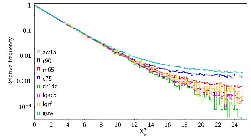
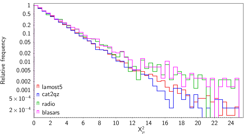
Figure 1: Relative frequencies of $X_{\mu}^{2}$ for the filtered matches to the catalogues in Table 1. The catalogues are identified by the codes given in column 6 of the table, with the eight larger catalogues in the upper panel and the smaller catalogues in the lower panel. The four radio catalogues (ICRF3 S/X, ICRF3 K, ICRF X/Ka, and OCARS) are combined under ‘radio’, and the three blasar catalogues (Roma-BZCAT, 2WHSP, and ALMA calibrators) are combined under ‘blasars’.

Applying this tool to the full sets of filtered matches to each external catalogue in Table 1 reveals that only the sources matched to three of the catalogues (C75, Milliquas v6.5, and Gaia-unWISE) show clear evidence of stellar contamination. These catalogues are marked with an asterisk in the table. The filtered matches of the remaining 14 catalogues show no obvious traces of stellar contamination and therefore qualify as being part of Gaia-CRF3.

The same Gaia source usually appears in the filtered cross-matches to several external catalogues. One reason for this, as discussed in Appendix B, is that many of the catalogues are at least partially based on the same observational material (the IR photometry of WISE, certain data releases of SDSS, etc.), although their criteria for the selection of QSOs may be different. But even when the observational material is different, it is no wonder that different approaches and algorithms result in strongly overlapping samples, namely if they tend to find the same objects. It is therefore reasonable to expect that the circumstance that a Gaia source has matches in several external catalogues increases the reliability of its classification as a QSO. If we split the set of Gaia sources matching a given external catalogue (after the astrometric filtering) into subsets that are present also in other catalogues and a subset that appears only in the cross-match with this particular catalogue, we can therefore use an analysis of these subsets to improve the purity of the final QSO selection.

Using this idea, we selected three sets of Gaia sources that appear only among the filtered matches of C75, Milliquas v6.5, and Gaia-unWISE, but do not appear in any of the other catalogues: we call these the c75-only, m65-only, and guw-only sets. All three sets show significant stellar contamination. We found no obvious way to clean the c75-only sources and this whole set of 95 988 sources was therefore dropped from further consideration. The Milliquas v6.5 and Gaia-unWISE catalogues include estimates of the probability that a source is a QSO. Selecting from the m65-only set only the sources with the highest probability of being a QSO did not remove the contamination and that set of 26 326 sources was therefore also dropped. For the guw-only set we found, on the contrary, that the subset of sources with the highest QSO probability ($\texttt{PROB\_RF}=1$) appears to be free of stellar contaminants. This gave an additional set of 229 914 sources for Gaia-CRF3. The other 491 894 guw-only sources were dropped (any relaxation of $\texttt{PROB\_RF}=1$ immediately gave samples with clear signs of stellar contamination). The number of sources from the cross-matches of each catalogue that passed also this second stage of astrometric filtering is given in the fifth column of Table 1, summing up to a total of 1 614 173 sources. The relative frequencies of $X_{\mu}^{2}$ in Gaia-CRF3 and in the three sets of sources dropped from C75, Milliquas v6.5, and Gaia-unWISE are shown in Fig. 2. Deviations from the exponential distribution expected for Gaussian errors are very obvious for the dropped sets; for the final selection the distribution is briefly discussed below (Sect. 2.4).

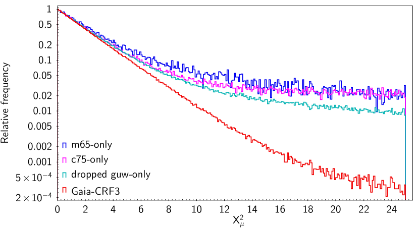
Figure 2: Relative frequencies of $X_{\mu}^{2}$ for the final selection of Gaia-CRF3 sources, and for the filtered matches to C75, Milliquas v6.5, and Gaia-unWISE that were dropped in the final selection.

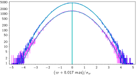
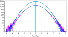
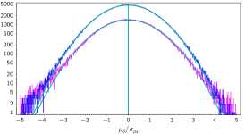
Figure 3: Distributions of the normalised parallaxes and proper motion components for the Gaia-CRF3 sources with five-parameter (blue) and six-parameter (magenta) solutions. The turquoise curves show the corresponding best-fit Gaussian distributions.

A separate investigation was done for the QSO candidates in the areas of the LMC and SMC, which have a very high density of confusion sources (Fig. 19) and therefore a higher risk of chance matches. The statistics of confusion sources in these areas are discussed in Appendix D. The Gaia-CRF3 contains 5411 and 2779 sources, respectively, in the LMC and SMC areas (as defined in the appendix). The distributions of the normalised quantities indicate a low level of stellar contamination in these sets.

Further checks of the selection were done by splitting the Gaia-CRF3 sources into subsets according to magnitude, colour, and Galactic or ecliptic latitude, and examining the distributions of normalised parallaxes and proper motions. No clear contamination was detected in any of the subsets.

Gaia-CRF3 contains only 195 sources with $\left|\,\sin b\,\right|<0.1$. They all come from the VLBI-based catalogues, for which Eqs. (4) and (5) were not applied. We made an attempt to find a clean set of QSO-like sources also in the Galactic plane area, that is without applying the criterion in Eq. (4). Using the cross-matches and the remaining four criteria, we found nearly 100 000 additional QSO candidates with $\left|\,\sin b\,\right|<0.1$. However, the distributions of their normalised parameters indicate a high level of stellar contamination. This demonstrates that the cross-matches and/or external astrophysical classifications are unreliable in this crowded part of the sky, and none of these sources were further considered for Gaia-CRF3. However, we note that this set should contain a significant percentage of genuine QSOs, part of which may be recovered in future versions of the Gaia-CRF (see Sect. 2.5).

2.4 Final selection

The union of all Gaia sources that passed both stages of the filtering contains 1 614 173 sources and constitutes the final source list of Gaia-CRF3. Of these, 1 215 942 (75%) have five-parameter solutions in Gaia EDR3 and 398 231 (25%) have six-parameter solution. Appendix C explains how to find the astrometric parameters of these sources and how to trace the matches of these sources in the external catalogues.

Figure 3 shows the distributions of the normalised parallaxes and proper motion components for both kinds of solutions. The standard deviations of the three normalised quantities are 1.052, 1.055, and 1.063 for the five-parameter solutions and 1.073, 1.099, and 1.116 for the six-parameter solutions. All distributions are very symmetric and close to the Gaussian shape (i.e. parabolic in the logarithmic plots), suggesting a low level of stellar contamination. The small excess of sources with normalised parameters beyond $\pm 4$ is not necessarily a sign of contamination, but could be produced by source structure or instrumental effects as well as by statistical fluctuations in the sample.

The number of (non-QSO) chance matches in Gaia-CRF3 can be estimated by counting the confusion sources that satisfy Eqs. (4) and (5) around positions that are slightly offset from the Gaia-CRF3 positions. Using offsets of $\pm 0.1$ deg in $\Delta\alpha\cos\delta$ or $\Delta\delta$ we conclude that Gaia-CRF3 is expected to contain up to 420 chance matches, of which 150 have five-parameter solutions and 270 have six-parameter solutions. This corresponds to a probable contamination of 0.012% and 0.068%, respectively, of the five- and six-parameter sources in Gaia-CRF3.

The chance matches are obviously not the only cause of stellar contamination in Gaia-CRF3. Further contaminants may come from erroneous classification of some sources in the external catalogues, even among the sources that passed the astrometric filtering in Eqs. (1)–(5). We have found no means to quantify this effect, but expect it to be quite small.

A certain hint on the possible (total) level of contamination could be given by the relative frequency of $X_{\mu}^{2}$ for Gaia-CRF3, as shown by the red curve in Fig. 2. This distribution can be rather well described as the mixture of two Gaussian distributions: one with standard deviation of 1.051 containing 98.0% of the sources, the other with standard deviation of 2.038 containing 2.0% of the sources. We stress that this cannot directly be interpreted in terms of the purity of the Gaia-CRF3: on one hand, genuine QSOs may show deviations from Gaussianity for other reasons (as mentioned above); on the other hand, some contaminants will have measured proper motion that are perfectly consistent with the extragalactic hypothesis. Nevertheless, we consider it unlikely that the level of contamination in Gaia-CRF3 is higher than 2%. Further investigations are needed to show if this claim is justified.

2.5 Discussion of the selection

Assuming that QSO-like sources have zero true values for the parallaxes and proper motions, and that the astrometric errors are Gaussian with uncertainties as given in Gaia EDR3, we expect that very few actual QSOs in a sample of a few million candidates will violate Eqs. (2) or (3). The numerical boundaries in Eqs. (2) and (3) were selected empirically, based on the data themselves, and represent a compromise taking into account possible non-Gaussian systematic errors and effects of complex and sometimes time-dependent source structure. The latter are to be expected for QSOs and could produce apparent proper motions over several years of observations, while parallaxes are much less affected by such effects. This justifies setting separate criteria for parallaxes and proper motions as described above. In future Gaia data releases, when these effects may be better known and statistically quantified, it will be possible to adopt a mathematically more consistent filtering approach based on the $3\times 3$ covariance matrix of the parallax and proper motion components.

As already mentioned, we expect that future versions of Gaia-CRF will to a higher degree depend on Gaia’s own (astrometric, photometric, and spectroscopic) observations, and that external catalogues of AGNs will consequently become less important for the selection of QSO-like sources. These catalogues will continue to be important for validation purposes, but their uses in the selection process may become more complex if the astrometry in external catalogues is already Gaia-based. For example, a criterion such as Eq. (5) may not be meaningful if the position in the external catalogue comes from a previous Gaia data release.

The search for the QSOs in the Galactic plane is an important scientific problem that requires further investigation. We note that more advanced methods to combine different datasets in the search for QSOs in the Galactic plane are under development (e.g., Fu et al. 2021). Combined with the expected use of Gaia’s own object classification, one can hope that these methods will result in a much improved completeness of the Gaia-CRF in the Galactic plane in the future.

The selection of QSO-like objects described here is mainly driven by the reliability of the resulting set of sources. The resulting set of QSO-like sources can be considered ‘reliable’, but by no means ‘complete’. It is clear that the selection algorithm rejects some genuine quasars, for example if they show observable mean proper motions for the time span of the Gaia EDR3 data. A prominent example here is 3C273 – the brightest quasar on the sky, which has significant proper motion in declination in Gaia EDR3 and $X_{\mu}^{2}=29.7$ (Eq. 3).

For the purposes of aligning the reference frame of Gaia EDR3 with the ICRF, and especially for ensuring that it has negligible spin with respect to distant galaxies, one can use a much smaller set of QSO-like sources than the full Gaia-CRF3 without significantly increasing the statistical uncertainties of the global system. Indeed, this system was defined in the final stages of the primary astrometric solution, as described in Sect. 5, using only about 0.4 million ‘frame rotation’ sources. However, the purpose of Gaia-CRF3 is not just to fix the system for the Gaia astrometric solution, but to provide the community with a direct access to this system with sources as faint as permitted by the sensitivity of Gaia, while still having a very low level of stellar contamination.

3 Statistical properties of the Gaia-CRF3 sources

In this section we present the overall properties of Gaia-CRF3 primarily in terms of its distributions in position, magnitude, colour, and astrometric quality.

3.1 Distribution of the sources on the sky

The spatial distribution of the ${\sim}1.6$ million Gaia-CRF3 sources is shown in Fig. 4. Their distributions in galactic longitude and latitude are shown in Fig. 5. In the avoidance zone $\left|\,\sin b\,\right|<0.1$ Gaia-CRF3 has only 195 sources matched to the radio catalogues as described in Sect. 2. Outside the avoidance zone the average density is about 42 deg^-2, but with significant variations with galactic latitude; the density is typically below average for $|\,b\,|\lesssim 30^{\circ}$ and above at higher latitudes. This comes from the source catalogues used in our compilation combined with the selection function in Eq. (4), designed to avoid stellar contaminants near the Galactic plane. From Fig. 18 one can see that also most of the external catalogues avoid crowded regions on the sky. We note that the density of Gaia-CRF3 reaches about 110 deg^-2 in some areas on the sky. Given the expected isotropic distribution of QSOs and the effects of Galactic extinction, a complete version of a Gaia-CRF could therefore potentially comprise about 4 million sources. This estimate is also suggested by recent studies (e.g. Shu et al. 2019; Bailer-Jones et al. 2019; Fu et al. 2021) of the QSOs as well as by the extragalactic results of Gaia DR3.

Table 2: Characteristics of the Gaia-CRF3 sources.

type	number	$G$	$G_{\text{BP}}-G_{\text{RP}}$	$\nu_{\rm eff}$	RUWE	$\sigma_{\text{pos,max}}$	$\sigma_{\mu\alpha*}$	$\sigma_{\mu\delta}$
of solution	of sources	[mag]	[mag]	[$\mu\text{m}^{-1}$]		[$\,{\mu}\text{as}$]	[$\,\mu\text{as\,yr}^{-1}$]	[$\,\mu\text{as\,yr}^{-1}$]
five-parameter	1 215 942	19.92	0.64	1.589	1.013	385	457	423
six-parameter	398 231	20.46	0.92	1.541	1.044	749	892	832
all	1 614 173	20.06	0.68	1.585	1.019	447	531	493

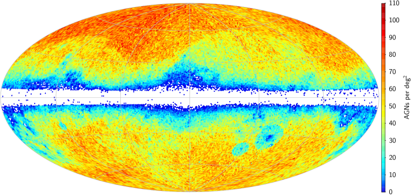
Figure 4: Sky distribution of the Gaia-CRF3 sources. The plot shows the density of sources per square degree computed from the source counts per pixel using HEALPix of level 6 (pixel size $\simeq 0.84$ deg²). The magnitude distribution and further properties of the sources are shown on Fig. 6. This full-sky map uses a Hammer–Aitoff projection in galactic coordinates, with $l=b=0$ at the centre, north up, and $l$ increasing from right to left.

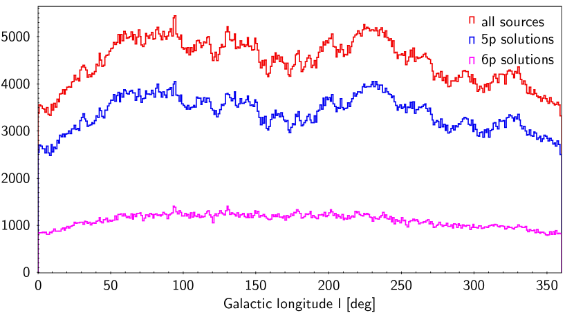
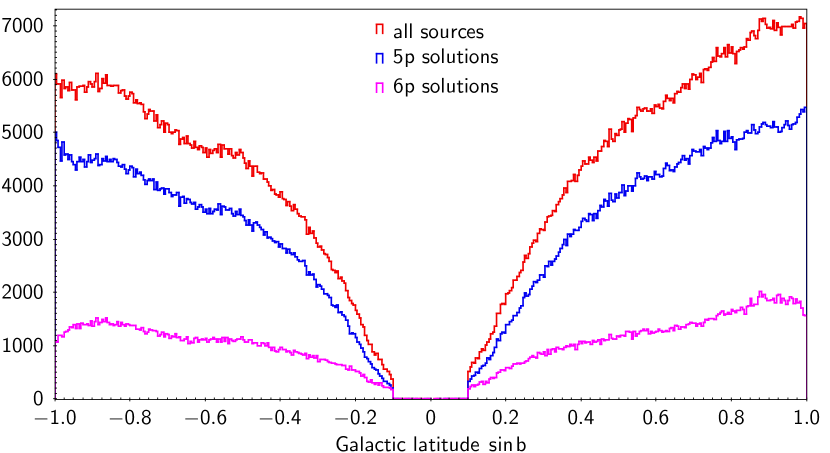
Figure 5: Distribution of the Gaia-CRF3 sources in galactic coordinates. There are only 195 sources in the avoidance zone $\left|\,\sin b\,\right|<0.1$. The distribution is shown for the whole Gaia-CRF3 and separately for the sources with five- and six-parameter astrometric solutions.

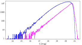
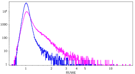
Figure 6: Histograms of some important characteristics of the Gaia-CRF3 sources with five-parameter solutions (blue) and six-parameter solutions (magenta). Left to right: $G$ magnitudes, colour index $G_{\text{BP}}-G_{\text{RP}}$, and the astrometric quality indicator RUWE.

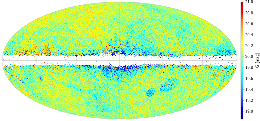
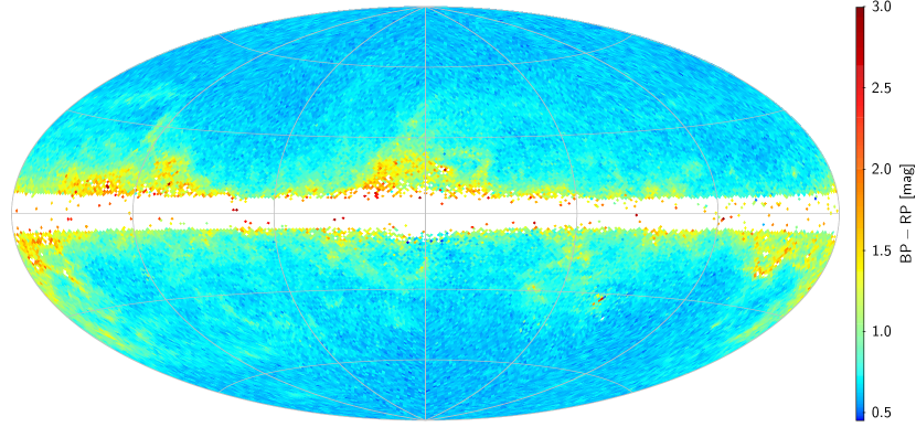
Figure 7: Median $G$ magnitude (top) and median colour index $G_{\text{BP}}-G_{\text{RP}}$ (bottom) of the Gaia-CRF3 sources. These maps use a Hammer–Aitoff projection in galactic coordinates, with $l=b=0$ at the centre, north up, and $l$ increasing from right to left.

3.2 Main characteristics of the sources

Table 2 and Fig. 6 show the median values and distributions of several important properties of the Gaia-CRF3 sources, split according to the nature of the solution (five- or six-parameter solution): magnitude ($G$), colour index ($G_{\text{BP}}-G_{\text{RP}}$), and the renormalised unit weight error (RUWE; Lindegren et al. 2021b). The RUWE is a measure of the goodness-of-fit of the astrometric model to the observations of the source. The expected value for a good fit is 1.0. A higher value could indicate that the source is not point-like at the optical resolution of Gaia (${\simeq}\,0.1\arcsec$), or that it has a time-variable structure. As seen in the left panel of Fig. 6, the proportion of six-parameter solutions increases for $G\gtrsim 19$, a feature that also implies that these sources are on average of lower astrometric accuracy, not only because they are fainter but also because the model fit is often worse, as shown in the right panel. The sources with six-parameter solutions are also on average redder (middle panel).

The sky distributions of the median magnitude $G$ and the colour index $G_{\text{BP}}-G_{\text{RP}}$ (Fig. 7) clearly show the effects of the Galactic extinction and reddening. We also see that the selection favours brighter sources in the crowded areas such as the Galactic plane and the LMC and SMC areas.

3.3 Astrometric parameters of the sources

The left panel of Fig. 8 shows the distribution of the formal positional uncertainty in Gaia-CRF3 separately for the five- and six-parameter solution. The positional uncertainty, $\sigma_{\text{pos,max}}$, is defined as the semi-major axis of the uncertainty ellipse (see Eq. (1) in Gaia Collaboration et al. 2018) at the reference epoch J2016.0. The middle panel is a scatter plot of $\sigma_{\text{pos,max}}$ versus $G$, with the smoothed median indicated by the dashed curve. In the right panel, the black curve (labeled ‘all sources’) gives the fraction of the full sky that has a density of Gaia-CRF3 sources exceeding the value on the horizontal axis. The other curves give the fractions when only sources with $\sigma_{\text{pos,max}}$ below a certain level are counted. In the 10% of the sky nearest to the Galactic plane ($\left|\,\sin b\,\right|<0.1$) the source density is negligible (cf. Fig. 4), which explains why none of the curves reaches above 90% sky coverage. To compute the fractions, the celestial sphere was divided into 49 152 pixels of equal area (${\simeq\,}0.8393\leavevmode\nobreak\ \text{deg}^{2}$, i.e. HEALPix level 6) and the density computed in each pixel. It should be noted that the curves therefore refer to the source densities at a spatial resolution of about 1 deg and would not be the same at a different resolution (pixel size). The plot shows, for example, that for a minimum density of 35 Gaia-CRF3 sources per square degree, about 62% of the sky could be covered; this fraction is reduced to 55% or 20% if we require, in addition, that $\sigma_{\text{pos,max}}$ is below 1.0 or 0.5 mas. Conversely, at 62% coverage there could be at least 30, 18, and 3 sources per square degree with $\sigma_{\text{pos,max}}<1$, 0.5, and 0.2 mas, if in each case the most populated pixels are chosen. The corresponding magnitude distributions can be gleaned from the scatter plot in the middle panel, where the different levels of positional uncertainty have been marked.

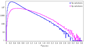
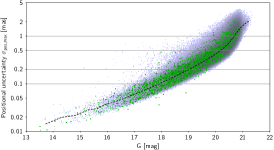
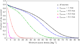
Figure 8: Positional uncertainty and source density distribution in Gaia-CRF3. Left: histogram of the positional uncertainty $\sigma_{\text{pos,max}}$ for Gaia-CRF3 sources with five-parameter solutions (blue) and six-parameter solutions (magenta). Middle: scatter plot of $\sigma_{\text{pos,max}}$ versus the $G$ magnitude. The dashed curve is the smoothed median uncertainty versus magnitude. The green points are the sources matched to ICRF3 S/X. Right: fraction of sky covered by a given minimum density of Gaia-CRF3 sources at different levels of positional uncertainty (see text for further explanation).

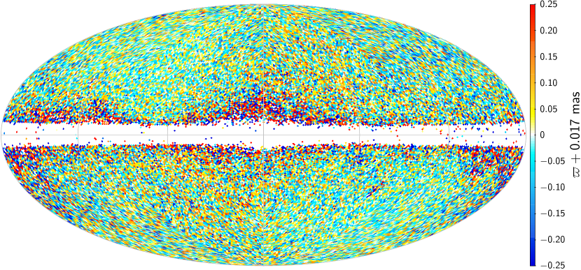
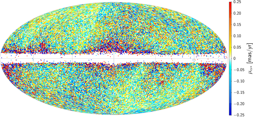
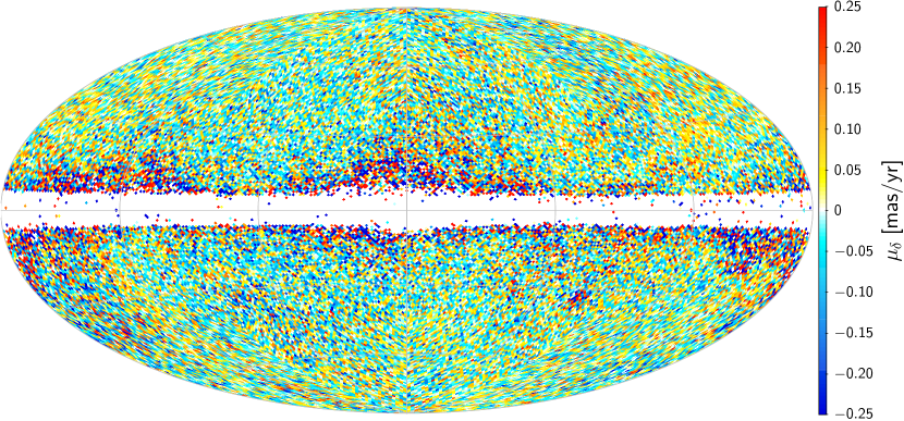
Figure 9: Sky distributions of the parallax $\varpi$ and the components of proper motion $\mu_{\alpha*}$ and $\mu_{\delta}$. Median values over the pixels of HEALPix level 6 (pixel size $\simeq 0.84$ deg²) are shown. These maps use a Hammer–Aitoff projection in galactic coordinates, with $l=b=0$ at the centre, north up, and $l$ increasing from right to left.

Figure 9 shows the distributions of the median parallax and proper motion components on the sky. Both large-scale systematics and small-scale inhomogeneities are visible in these maps. The large-scale systematics are discussed in Sect. 3.4. Small-scale inhomogeneities, seen as fluctuating median values between neighbouring HEALPix cells in the maps, are mainly caused by the statistical scatter of the astrometric parameters in each cell. They are generally stronger in areas of low source density (Fig. 4) or fainter median magnitude (Fig. 7, top), and also in the ecliptic belt (ecliptic latitude $\left|\,\beta\,\right|\lesssim 45^{\circ}$), where the scanning law usually results in less accurate astrometric solutions than at high ecliptic latitudes (see, for example, Sect. 5.4 and Figs. 8 and 9 in Lindegren et al. 2021b). Numerous streaks, edges, and other small-scale features can also be traced to the scanning law. The overall scatter of the median values in the three maps is about 0.11 mas ($\varpi$), 0.12 $\,\text{mas\,yr}^{-1}$ ($\mu_{\alpha*}$), and 0.11 $\,\text{mas\,yr}^{-1}$ ($\mu_{\delta}$), if only the cells with at least five QSOs are counted (covering 85% of the sky). The positional errors are expected to be of a roughly similar size as the parallax scatter. Thus, we conclude that Gaia-CRF3, on an angular scale of about $1^{\circ}$ and over most of the sky, defines a local reference frame accurate to better than 0.2 mas in position and 0.2 $\,\text{mas\,yr}^{-1}$ in proper motion.

3.4 Systematic errors

Systematic errors in Gaia-CRF3 were discussed already in Lindegren et al. (2021b, Section 5.6). In particular, the left column of their Fig. 13 contains smoothed maps of the parallaxes and proper motions of the Gaia-CRF3 sources that have five-parameter astrometric solutions. These maps were obtained by a special smoothing procedure applied to the parameters of the individual sources. Including also the less numerous and fainter sources with six-parameter solutions does not noticeably change these maps.

Here we present the results of a different way to analyse systematics in the Gaia-CRF3 proper motions, namely by fitting an expansion of vector spherical harmonics (VSH; Mignard & Klioner 2012) up to a certain degree $\ell$. Although the VSH provide a smooth model of the systematic errors also in the regions where only a few sources are present, such as in the Galactic plane, the higher-degree harmonics ($\ell\gtrsim 15$) are only weakly constrained in these areas, resulting in unreliable estimates of the VSH coefficients also in other parts of the sky because of the global scope of the fitted VSH functions.

Analogous to the discussion of parallax systematics in Sect. 5.7 of Lindegren et al. (2021b), using (scalar) spherical harmonics, the VSH allow us to estimate the angular power spectrum of the systematics in the Gaia-CRF3 proper motions. To this end we used the set of 1 215 942 Gaia-CRF3 sources with five-parameter solutions. Given the vector field of proper motions of those sources we computed the VSH expansion as given by Eq. (30) of Mignard & Klioner (2012), including all the terms of degree $1\leq\ell\leq L$. It was found that the VSH fit is reasonably stable for $L\leq 12$. When higher degrees are included, the fits become questionable, mainly because of the inhomogeneous distribution of the sources on the sky (see Sect. 3.1 above and Figs. 3 and 4 of Gaia Collaboration et al. 2021b). All subsequent computations used $L=12$. The fitted VSH coefficients confirmed the maps of systematic errors in proper motion shown on Fig. 13 of Lindegren et al. (2021b). From the same coefficients we obtained the powers $P^{t}_{\ell}$, $P^{s}_{\ell}$ of the toroidal and spheroidal signals of degree $\ell$, as defined by Eq. (76) of Mignard & Klioner (2012). The total power of degree $\ell$ is $P_{\ell}=P^{t}_{\ell}+P^{s}_{\ell}$. The mean powers of the toroidal and spheroidal harmonics of degree $\ell$ are then $C^{t}_{\ell}=P^{t}_{\ell}/(2\ell+1)$ and $C^{s}_{\ell}=P^{s}_{\ell}/(2\ell+1)$, where $2\ell+1$ is the number of harmonics at the degree $\ell$. This is fully analogous to the definitions for the scalar spherical harmonics given by Eq. (31) of Lindegren et al. (2021b).

We note that the VSH components of degree $\ell=1$ in the proper motions should be analysed separately from other systematic effects. The toroidal harmonic of degree $\ell=1$ represents a residual spin of the reference frame, and should in principle be negligible thanks to the way the reference frame is constructed (see Sect. 5 below). The spheroidal harmonic of degree $\ell=1$ represents a ‘glide’ component of the proper motions that is expected as a consequence of the acceleration of the Solar system in the rest frame of remote sources (Gaia Collaboration et al. 2021b). Although these terms need to be included in the VSH fit, the subsequent discussion of systematics in the Gaia-CRF3 proper motions only considers the VSH components of degree $\ell=2,\dots,12$.

Formally, the powers and the mean powers are weighted sums of the squared VSH coefficients. Appendix A of Gaia Collaboration et al. (2021b) demonstrates that such quantities are biased (overestimated) when the VSH coefficient are estimated in a least squares fit. Equation (A.1) of that Appendix gives the exact formula to correct the bias. In particular, the corrected (unbiased) values of the mean powers are

$$\hat{C}_{\ell}^{t} = C_{\ell}^{t}-N_{\ell}^{t}\,,$$ (6)

$$\hat{C}_{\ell}^{s} = C_{\ell}^{s}-N_{\ell}^{s}\,,$$ (7)

where the noise corrections $N_{\ell}^{t}$ and $N_{\ell}^{s}$ are obtained by the same formulas as $C_{\ell}^{t}$ and $C_{\ell}^{s}$ but using the uncertainties of the VSH coefficients instead of the coefficients themselves. Explicit computations for the present data show that $N_{\ell}^{t}\simeq N_{\ell}^{s}\simeq 3.44-0.07\,\ell-0.01\,\ell^{2}\leavevmode\nobreak\ \mu\text{as}^{2}\,{\text{yr}}^{-2}$ ($2\leq\ell\leq 12$).

Figure 10 shows the corrected estimates $\hat{C}^{t}_{\ell}$ and $\hat{C}^{s}_{\ell}$ for $\ell=2,\dots,12$. The ragged shape of (especially) the toroidal spectrum is very real, as shown by the error bars. One sees that the toroidal powers are substantially larger than the spheroidal ones for the odd degrees, while they are more similar for even degrees. We have no explanation for this but presume it is related to the specific parameters of the scanning law and basic angle.

In analogy with Eq. (32) of Lindegren et al. (2021b), it is convenient to consider the cumulative characteristics

$$R^{t}(\ell_{\text{max}}) = \sqrt{{1\over 4\pi}\sum_{\ell=2}^{\ell_{\text{max}}}(2\ell+1)\,\hat{C}_{\ell}^{t}}\,,$$ (8)

$$R^{s}(\ell_{\text{max}}) = \sqrt{{1\over 4\pi}\sum_{\ell=2}^{\ell_{\text{max}}}(2\ell+1)\,\hat{C}_{\ell}^{s}}\,,$$ (9)

$$R(\ell_{\text{max}}) = \sqrt{{1\over 4\pi}\sum_{\ell=2}^{\ell_{\text{max}}}(2\ell+1)\,\left(\hat{C}_{\ell}^{t}+\hat{C}_{\ell}^{s}\right)}\,$$ (10)

quantifying the RMS variations of the toroidal, spheroidal and total proper motion systematics on angular scales $\gtrsim 180^{\circ}/\ell_{\text{max}}$ (Fig. 11). We note that the toroidal components completely dominate the systematics for $\ell\geq 5$.

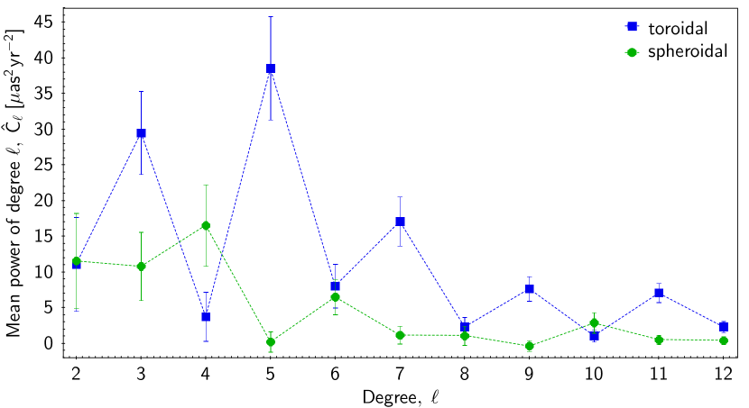
Figure 10: Corrected mean toroidal and spheroidal powers $\hat{C}^{t}_{\ell}$ and $\hat{C}^{s}_{\ell}$ of the systematics in proper motions of the Gaia-CRF3 sources with five-parameter solutions. The error bars show the $\pm 1$ standard deviation of each point, calculated on the assumption that the $2\ell+1$ contributing VSH coefficients have Gaussian errors.

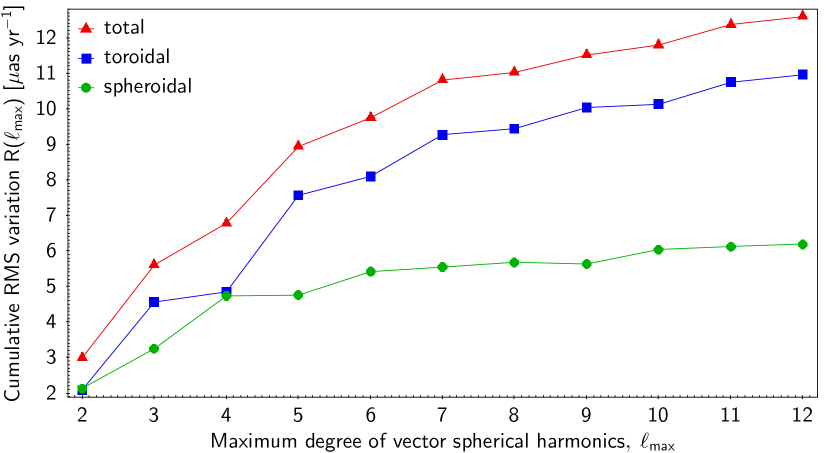
Figure 11: Corrected cumulative angular power spectrum of the systematic in proper motions of the Gaia-CRF3 sources with five-parameter solutions.

Summarising all this information we can claim that the frame-independent RMS of the vector field representing systematic errors in proper motions is $\lesssim 12$ $\,\mu\text{as\,yr}^{-1}$down to angular scales of ${\sim\,}15^{\circ}$. This level of systematic errors is low compared to the random errors of individual sources given in Table 2 and made it possible to reliably measure the subtle physical effect of the acceleration of the Solar system in Gaia EDR3 (Gaia Collaboration et al. 2021b).

4 Gaia-CRF3 counterparts of ICRF3 sources

Radio-loud sources in Gaia-CRF3 deserve special attention as they provide a direct link between the ICRF implementations in the radio and optical regimes. In this section we focus on the properties of the Gaia-CRF3 sources matched to ICRF3 (Charlot et al. 2020) and a statistical comparison of the optical and radio positions.

4.1 Statistics of ICRF3 sources in Gaia-CRF3

Gaia-CRF3 contains a total of 4723 radio-loud sources, of which 3181 are optical counterparts of radio sources in ICRF3 (Charlot et al. 2020), while an additional 1542 sources are found only in OCARS. Because the ICRF3 sources have the best quality of the astrometry in the radio domain and represent the official realisation of the ICRF in the radio, we restrict the discussion in this section to the 3181 Gaia-CRF3 sources in common with ICRF3. This set is the union of 3142, 660, and 576 sources matching the ICRF3 sources in the S/X, K, and X/Ka bands, respectively (69.3%, 80.1% and 85.0% of the corresponding catalogues). Most of the analysis below is further limited to the 3142 sources in ICRF3 S/X. Very few additional Gaia EDR3 sources are found only in the K or X/Ka bands of the ICRF3 (24 and 31 sources, respectively), and their overall properties are not too different from those of the S/X set.

From the sky distribution of the 3181 ICRF3 sources in Gaia-CRF3 (Fig. 12) we see that a band along the Galactic plane and the region with $\delta<-30^{\circ}$ (part of the fourth quadrant of the map in the Galactic coordinates) are underpopulated. This reflects the strong optical extinction in the Galactic plane and the fact that ICRF3 itself has a lower density of sources for $\delta<-30^{\circ}$.

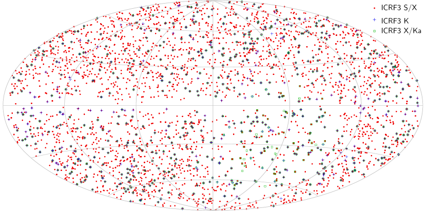
Figure 12: Distribution of the ICRF3 sources in Gaia-CRF3 in Galactic coordinates. Sources from ICRF3 S/X are shown by red dots, from ICRF3 K by blue crosses, and from ICRF3 X/Ka by turquoise squares. This map uses a Hammer–Aitoff projection in galactic coordinates, with $l=b=0$ at the centre, north up, and $l$ increasing from right to left.

The left panel in Fig. 13 shows the magnitude distribution of the 3142 Gaia-CRF3 sources in common with ICRF3 S/X and for the subset of 259 sources that are defining sources in ICRF3. As expected, there is no marked difference between the two sets, since the optical brightness plays no role in the ICRF3 selection of defining sources. The median $G=18.9$ is about one magnitude brighter than for the whole Gaia-CRF3 (Table 2).

The central panel in Fig. 13 shows the distribution of the positional uncertainty $\sigma_{\text{pos,max}}$ in Gaia-CRF3 for the same selections. The median uncertainty is 194 $\,{\mu}\text{as}$ for the whole set of ICRF3 S/X sources, and 162 $\,{\mu}\text{as}$ for the defining sources. These values are less than one half of the median positional uncertainty in the full Gaia-CRF3 sample, which can be attributed to their different distributions in $G$. Indeed, as shown by the middle panel of Fig. 8, the ICRF3 sources follow the same general variation of $\sigma_{\text{pos,max}}$ with $G$ as other Gaia-CRF3 sources. In other words, nothing in the Gaia astrometry suggests that the ICRF3 are better or worse than other Gaia-CRF3 sources of comparable magnitude.

The right panel in Fig. 13 shows the distribution of the positional uncertainty in the radio domain for the same sources. By coincidence, the median positional uncertainty of the 3142 sources in ICRF3, 197 $\,{\mu}\text{as}$, is practically the same as in Gaia-CRF3. For the subset of defining sources, however, the positional uncertainties in ICRF3 are much smaller (the median is 39 $\,{\mu}\text{as}$), as these sources were selected precisely for their high radio-astrometric quality. In Gaia-CRF3 the defining sources are only marginally more accurate than the non-defining sources, consistent with the former being, on average, about 0.2 mag brighter (cf. Fig. 13, left panel).

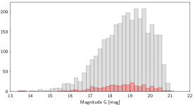
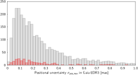
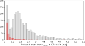
Figure 13: Distribution of magnitudes and formal positional uncertainties for the sources common to Gaia-CRF3 and ICRF3 S/X. The full set of 3142 sources is shown by the grey histograms, and the 259 defining sources by the red histograms. Left: distribution of magnitudes $G$. Middle: distribution of positional uncertainties in Gaia EDR3. There are 126 sources with $\sigma_{\text{pos,max}}^{\text{EDR3}}>1$ mas, of which eight are defining sources in ICRF3. Right: distribution of positional uncertainties in ICRF3 S/X. There are 155 sources with $\sigma_{\text{pos,max}}^{\text{ICRF3}}>1$ mas, of which one is a defining source.

4.2 Positional differences

We now compare the individual positions of ICRF3 S/X sources in ICRF3 and Gaia-CRF3. Thanks to the high positional accuracy in both catalogues and the small cross-matching radius $\Delta_{\text{max}}=100$ mas used, cross-matching errors between the two catalogues are highly unlikely and we can assume that the optical and radio emissions being compared originate in broadly the same extragalactic object. Positional differences $\Delta\alpha{*}=(\alpha_{\text{EDR3}}-\alpha_{\text{ICRF3}})\cos\delta$ and $\Delta\delta=\delta_{\text{EDR3}}-\delta_{\text{ICRF3}}$ are computed after propagating the ICRF3 positions from the ICRF3 epoch (J2015.0) to the Gaia-CRF3 epoch (J2016.0), using the precepts described in Charlot et al. (2020, Section 5.3); this takes into account the small shifts ($\lesssim 5\,\,{\mu}\text{as}$) expected from the Galactic acceleration.

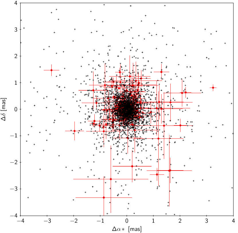
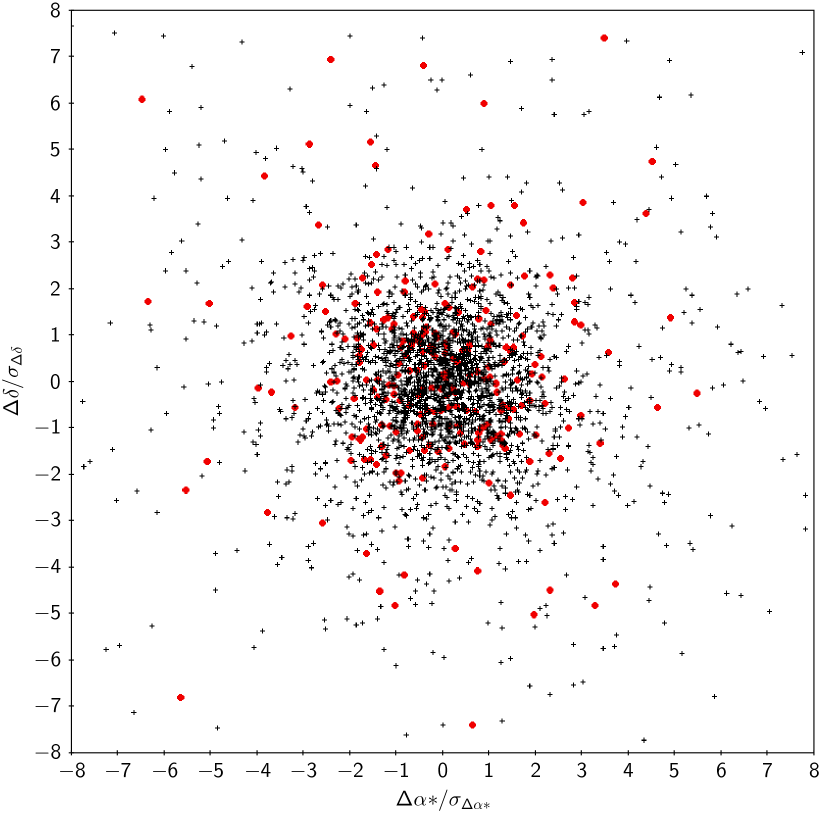
Figure 14: Positional differences in $\alpha$ and $\delta$ between Gaia-CRF3 and ICRF3 S/X for the 3142 common sources. The 259 defining sources in ICRF3 are shown as filled red circles, other sources as black crosses. Top: differences in mas. Errors bars representing the quadratically combined uncertainties in the two catalogues are shown only for the defining sources. Bottom: the same differences divided by the quadratically combined uncertainties in the two catalogues. No error bars are shown in this plot, as they would all be $\pm 1$ unit.

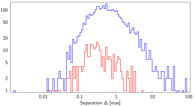
Figure 15: Histograms of the separations $\Delta$ between Gaia-CRF3 and ICRF3 S/X for the full set of 3142 common sources (blue; the median is 0.516 mas) and the 259 defining sources (red; the median is 0.292 mas).

The top panel of Fig. 14 is a scatter diagram of the positional differences. Of the 3142 sources, 127 (4%) have a positional difference $>4$ mas in either coordinate and fall outside the boundaries of the plot. The median separation $\Delta=(\Delta\alpha{*}^{2}+\Delta\delta^{2})^{1/2}$ is 0.516 mas for all 3142 sources, and 0.292  mas for the 259 defining sources (Fig. 15).

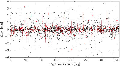
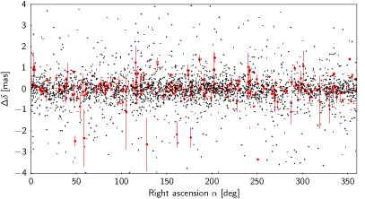
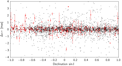
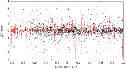
Figure 16: Positional differences between Gaia-CRF3 and ICRF3 S/X versus $\alpha$ (top) and $\sin\delta$ (bottom). Defining sources in ICRF3 are shown as filled red circles, with errors bars representing the combined positional uncertainties in the two catalogues; other sources are shown as black crosses.

The distributions of $\Delta\alpha{*}$ and $\Delta\delta$ are roughly symmetric around zero with a median offset of $+4\,\,{\mu}\text{as}$ in right ascension and $-6\,\,{\mu}\text{as}$ in declination. Similarly, the scatter diagrams of the positional differences versus right ascension and declination (Fig. 16) show no significant systematics or trends in either coordinate. The distributions are very regular with a pronounced central concentration of width below 1 mas, plus a scatter of several hundred outliers at several mas. Furthermore, an analysis of the positional differences using VSH does not reveal any significant systematic effects. The statistical significance of the fitted coefficients is low, while the largest effects represented by the VSH expansion are located in the areas with low source density (around the Galactic plane and for $\delta<-30^{\circ}$).

The lower panel of Fig. 14 shows the same position differences as in the upper panel, but normalised by the quadratic combination of the uncertainties in the ICRF3 and Gaia-CRF3 catalogues. If the optical and radio centres of emission coincided, we would expect the normalised position differences to follow a normal distribution with standard deviation only slightly above 1.0. In fact, the distributions are significantly wider (the RSE is 1.92 in right ascension and 1.80 in declination), with fatter tails than expected for a Gaussian: 225 sources fall outside the plotted frame, and more than 100 are outside $\pm 5\times\text{RSE}$ in each coordinate.

Both in ICRF3 and in Gaia-CRF3 there are significant correlations between the errors in right ascension and declination, and a useful statistic that takes this into account is

$$X_{\Delta}^{2}\equiv\begin{bmatrix}\leavevmode\nobreak\ \Delta\alpha{*}&&\Delta\delta\leavevmode\nobreak\ \end{bmatrix}\,\text{Cov}(\mbox{\boldmath$\Delta$})^{-1}\begin{bmatrix}\leavevmode\nobreak\ \Delta\alpha{*}\\[6.0pt] \Delta\delta\end{bmatrix}\,,$$ (11)

where $\text{Cov}(\mbox{\boldmath$\Delta$})$ is the covariance matrix given by Eq. (20). This is completely analogous to the statistic $X_{\mu}^{2}$ for the proper motions, defined in Eq. (3), and like $\Delta$ it is independent of the reference frame used. The distributions of $X_{\Delta}^{2}$ are shown in Fig. 17. For Gaussian errors we expect exponential distributions. The dashed lines are the functions $1450\exp[-\frac{1}{2}(X_{\Delta}/1.3)^{2}]$ and $120\exp[-\frac{1}{2}(X_{\Delta}/1.3)^{2}]$ fitted by eye to the inner parts of the histograms ($X_{\Delta}^{2}\lesssim 10$). The integrals of these exponential are 2450.5 and 202.8, that is 78% of respective sample. One possible interpretation of this is that the (combined) uncertainties are generally underestimated by a factor 1.3, and that about 22% of the objects in the samples have radio–optical positional offsets that are statistically significant at the current level of accuracy in the two catalogues; this fraction is, moreover, the same for the defining sources as for the full sample. Using a criterion such as $X_{\Delta}^{2}>25$ to pick out the individual sources that have a significant offset yields 433 sources, 36 of which are defining ones, or 14% of the respective samples. The angular offsets of these sources range from 0.17 mas to tens of mas, with a median value of 2.3 mas for the 433 sources from the full sample, and 0.84 mas for the 36 defining sources.

We note that the median $X_{\mu}^{2}$ is slightly higher (2.36) for the 433 sources with $X_{\Delta}^{2}>25$ than for the full sample of 3142 sources (1.82). This could indicate that the positional offsets are not constant over the time scale of the Gaia observations.

These results confirm and amplify the conclusion reached already with Gaia DR1 and Gaia DR2, namely that radio–optical offsets are significant for a large fraction of the ICRF3 sources. The correlation with jets has been well established, for example by Petrov et al. (2019) and Plavin et al. (2019), and the physical signature of offsets is also supported in the studies by Lambert et al. (2021) and Liu et al. (2021).

The question now is therefore not so much the existence of such offsets but rather what consequences they have for the relation between the radio and optical frames. A plain match between the two catalogues leaves sources with true differences in position, much larger than the expected random scatter. These differences will not decrease with future versions of the radio and optical frames. Although this does not impact the quality of either realisation, it could limit the attainable accuracy of their mutual alignment. To circumvent this problem, specific procedures may be required, such as the selection of a common set of reference sources for the alignment. More generally, the importance of physical deviations between the reference frames at different wavelength bands needs to be better understood. This problem will be even more important for the future high-accuracy astrometric observations in the near infrared (Hobbs et al. 2021).

A closely related question concerns the interpretation and use of the reference frame at different epochs. ICRF3 is the first realisation of the VLBI frame that has an epoch (2015.0) and an official procedure to transform from this epoch to another (Charlot et al. 2020). The reason for the epoch transformation is the effect of the acceleration of the Solar system relative to the remote celestial sources, often referred to as ‘Galactic acceleration’, although it may contain other components as well. If ignored, the Galactic acceleration will slowly distort the frame at a rate of about 6 $\,\mu\text{as\,yr}^{-1}$. The effect should therefore be taken into account when comparing ICRF3 with the Gaia-CRF, as was indeed done for this paper. The transformation depends on three parameters that can be determined by observation; for ICRF3, however, a set of fixed values are specified. In case of Gaia, full astrometric solutions including parallaxes and proper motions are computed for all Gaia-CRF sources. Each version of Gaia-CRF has a particular epoch common to that of the astrometric catalogue of the corresponding Gaia DR; for Gaia-CRF3 this is 2016.0. No specific correction for the Galactic acceleration is applied or recommended for Gaia-CRF. However, the effect is implicitly contained in the measured proper motions and a normal epoch transformation would take also this effect into account, albeit with a positional accuracy that degrades with the epoch difference. In Gaia Collaboration et al. (2021b) the components of the acceleration of the Solar system were determined from the proper motions of Gaia-CRF3. Although that determination differs from the ICRF3 prescription by less than 1 $\,\mu\text{as\,yr}^{-1}$, there thus is a conceptual difference between how the effect is treated in the two reference frames.

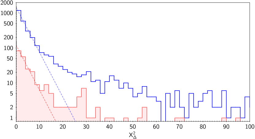
Figure 17: Histograms of the normalised separations $X_{\Delta}^{2}$ between Gaia-CRF3 and ICRF3 S/X for the full set of 3142 common sources (blue) and the 259 defining sources (red). The dashed curves are the exponential functions described in the text. A total of 195 sources have $X_{\Delta}>10$ and fall outside this plot (10 of them are defining sources in ICRF3).

5 Use of Gaia-CRF3 sources in the frame rotator of AGIS 3.2

In the astrometric core solution for Gaia (the Astrometric Global Iterative Solution, AGIS; Lindegren et al. 2012), the frame rotator ensures that the reference frame of the astrometric solution complies, in a global sense, with the ICRS requirements. The frame rotator uses a pre-selected set of QSO-like sources, including optical counterparts of ICRF3 sources, to estimate the six rotation parameters (spin and orientation) for the solutions obtained in successive iterations, and corrects them in such a way that the QSO-like sources have no net rotation and are globally aligned with the ICRF3 sources.

The frame rotator sources are a subset of the much larger set of primary sources (about 14.3 million for EDR3) that contribute to the estimation of attitude, calibration, and global parameters in AGIS. Special selection rules apply to the primary sources; in particular, they must have colour information from Gaia’s BP and RP photometers of adequate quality for the calibration of colour-dependent instrumental effects. The selection of primary sources, including the frame rotator sources, is revised with each new release of astrometric data, but for logistic reasons it is mainly based on the astrometric and photometric data of the previous release. Thus, for Gaia EDR3 the selection of frame rotator sources was primarily based on the 556 869 QSO-like sources, including 2820 ICRF3 counterparts, that constitute the Gaia-CRF2 (Gaia Collaboration et al. 2018). However, not all of them had adequate colour information or passed the more stringent astrometric criteria for primary sources in Gaia EDR3, and the number of frame rotator sources used for EDR3 is therefore substantially smaller (429 249 sources). All of them have five-parameter solutions in Gaia EDR3 and were filtered by a procedure similar to the one used for Gaia-CRF3 but using a preliminary version of the Gaia EDR3 catalogue known as AGIS 3.1 (Lindegren et al. 2021b).

Details of the frame rotator as used for Gaia EDR3 are given in Appendix E. As described in the appendix, the orientation ($\varepsilon$) and spin ($\omega$) are estimated by separate least-squares solutions to the position differences of the ICRF3 sources (for the orientation) and to the proper motions of the many more QSO-like sources (for the spin). The algorithm includes an iterative procedure to identify and eliminate outliers, that is sources that deviate very significantly from the overall fit in one or both coordinates. Thus, we need to distinguish between the sources that were ‘considered’ by the algorithm, and the subset of non-outliers that was actually ‘used’ to determine the orientation or spin. The auxiliary table gaiaedr3.frame_rotator_source in the Gaia Archive lists the 429 249 frame rotator sources for Gaia EDR3 and contains flags to indicate which of them were considered and used for the orientation and spin solutions. As specified in the table, 428 034 of the sources considered for the spin were actually used to determine the spin in the final iteration of the primary solution, while 1215 (0.3%) were rejected as outliers. Of the 2269 sources with counterparts in ICRF3 S/X considered for the orientation, 2007 sources were actually used to determine the orientation, while 262 (11.5%) were rejected as outliers. Eight of the sources were rejected in both the spin and orientation solutions.

Because the preliminary AGIS 3.1 astrometry had to be used to select the frame rotator sources, it turns out that 46 of the latter do not pass the stricter criteria for the Gaia-CRF3 selection described in Sect. 2. These sources are thus listed in gaiaedr3.frame_rotator_source although they are not part of the Gaia-CRF3. This slight inconsistency has minimal impact on the resulting reference frame, as only two of the 46 sources were accepted by the frame rotator algorithm for the determination of the spin, and none of them for the determination of the orientation.

If the frame rotator algorithm is applied to this subset of sources, using the astrometric data as given in Gaia EDR3, the resulting estimates of the orientation and spin vectors are not strictly zero, as might be expected. For the spin, we obtain $\left|\,\mbox{\boldmath$\omega$}\,\right|\simeq 0.8\,\,\mu\text{as\,yr}^{-1}$ with an uncertainty of about $0.4\leavevmode\nobreak\ \,\mu\text{as\,yr}^{-1}$ in each axis; for the orientation, the result is $\left|\,\mbox{\boldmath$\varepsilon$}(2016.0)\,\right|\simeq 6.2\leavevmode\nobreak\ \,{\mu}\text{as}$ with an uncertainty of about $7\leavevmode\nobreak\ \,{\mu}\text{as}$ per axis. These deviations from zero can be traced to small differences in the positions and proper motions between the last iteration of the primary solution and the secondary source updates, from which the final data are taken. The reason for this (undesirable) effect is currently under investigation.

If the same algorithm is instead applied to the full set of Gaia-CRF3 sources, the result for the spin is

$$\mbox{\boldmath${\omega}$}=\begin{bmatrix}-3.44\pm 0.30\\ +1.57\pm 0.28\\ -1.24\pm 0.32\end{bmatrix}\leavevmode\nobreak\ \text{$\mu$as\leavevmode\nobreak\ yr${}^{-1}$,}$$ (12)

in which 1 607 289 (99.6%) of the sources are accepted; for the orientation correction the result is

$$\mbox{\boldmath${\varepsilon}$}(2016.0)=\begin{bmatrix}+3.41\pm 6.71\\ +8.99\pm 6.50\\ -1.47\pm 6.04\end{bmatrix}\leavevmode\nobreak\ \text{$\mu$as,}$$ (13)

in which 2738 (87.1%) of the 3142 ICRF3 S/X sources are accepted. Generally speaking, the result is sensitive to the precise selection of sources at the level of a few $\,\mu\text{as\,yr}^{-1}$ in spin and several $\,{\mu}\text{as}$ in the orientation.

6 Conclusions and prospects

In this paper we have reported on the construction and properties of the Gaia-CRF3, a celestial reference frame materialised in the optical domain resulting from the Gaia all-sky survey. Although built on only 33 months of data (from August 2014 to May 2017), the astrometric accuracy is already very similar to what was expected for the 5-year nominal mission, and with a larger set of QSOs than originally anticipated.

The Gaia-CRF3 consists of an astrometric catalogue of more than 1.6 million QSOs selected using a number of existing catalogues, with further filtering based on the Gaia data to ensure that the sample is as much as possible free of stellar contaminants. The $G$ magnitude extends from ${\sim\,}13$ to ${\sim\,}21$ mag, with a peak density at $G\simeq 20.5$ mag. The formal uncertainty is primarily ruled by the $G$ magnitude, with a typical precision of 1 mas at $G=20.6$, 0.4 mas at $G=20$ and 0.1 mas at $G=17.9$. There are 32 000 sources with formal position uncertainty ${<\,}0.1$ mas and 210 000 with ${<\,}0.2$ mas. Gaia-CRF3 is aligned to the radio ICRF3 by minimising the position differences for about 2000 common sources with high-quality solutions.

The comparison with ICRF3 shows that the floor formal accuracies are comparable in the optical and radio domains and better than 0.05 mas for the best measured sources. However the normalised positional differences are not compatible with a standard normal distribution and an estimated ${\sim\,}20\%$ of the common sources have statistically significant positional radio–optical offsets. For many sources, if not all, these offsets are probably real, although this is hard to prove without a detailed investigation at the source level (Petrov et al. 2019; Plavin et al. 2019). The radio and optical CRFs are both internally very consistent and materialise the ICRS in their respective wavelength range, but in view of the detected offsets it remains unclear how much their mutual consistency can be improved without a better knowledge of the physical processes responsible for the light and radio emissions. It is hoped that high-resolution observations and improved radio and optical positions will further characterise these offsets and lead to a better understanding of the underlying mechanisms (Johnson et al. 2019).

It should be understood that Gaia-CRF3 is entirely defined by the Gaia EDR3 data for the $\sim\,$1.6 million QSO-like sources discussed in this paper. These data include not only the barycentric positions of the sources at the reference epoch 2016.0, but also their proper motions (and parallaxes). Although individually insignificant in the vast majority of cases, these data provide invaluable information on the quality of the data and on possible systematic effects in the reference frame, both of instrumental and astrophysical origin. The reference frame defined by the proper motions of the Gaia-CRF3 sources is globally non-rotating at a level of a few $\,\mu\text{as\,yr}^{-1}$. It is not possible to quantify more precisely than this how well the Gaia-CRF3 complies with the ‘no rotation’ condition, because different subsets of the Gaia-CRF3 lead to determinations of the spin that differ on this level, which is also consistent with the estimated RMS level of systematics on large angular scales (low values of $\ell_{\text{max}}$) depicted in Fig. 11. As mentioned in Sect. 1, the secondary frame defined by the positions and proper motions of stars in Gaia EDR3, in particular at bright magnitudes, may have significantly higher systematics.

Gaia-CRF3 is by far the best realisation to date of the celestial reference frame in the visible. It meets the ICRS requirements for a realisation based on extragalactic sources. The IAU, during its XXXIst General Assembly in August 2021, resolved (Resolution B3) that ICRF3 at radio wavelengths and Gaia-CRF3 in the optical are realisations (ICRF) of the International Celestial Reference System (ICRS) to be used as a fundamental standard in their respective domain.

A new version of the Gaia-CRF comes out with every release of a new astrometric solution based on a larger volume of Gaia data. The current version, Gaia-CRF3, is common to Gaia EDR3 and Gaia DR3, for which the basic astrometric data are identical. Two more releases are expected, Gaia DR4 based on 66 months of observations, and Gaia DR5 using up to 120 months of data. The positional accuracy improves roughly as $T^{-1/2}$, where $T$ is the time baseline, leading to an improvement by almost a factor two for the final version compared with Gaia-CRF3.

It is expected that the systematics will also be improved in the future releases, although this cannot easily be quantified. A dramatic illustration of the improvement from Gaia-CRF2 to Gaia-CRF3 is the successful use of the latter to determine the acceleration of the Solar System (Gaia Collaboration et al. 2021b). Of paramount importance for the quality of the reference frame is the accuracy of proper motions, which impacts both the astrometric filtering of the sources (thus reducing stellar contamination) and the accuracy of the positions at earlier and later epochs. Proper motions generally improve as $T^{-3/2}$, which could give a factor seven more precise proper motions in the final release. Corresponding improvements can be expected for the determination of the reference frame (especially, its spin) as well as for the various physical effects that may be seen in the proper motions (e.g. the solar system acceleration; see Sect. 8 in Gaia Collaboration et al. 2021b for a brief discussion of other effects).

As mentioned in Sect. 3, up to 4 million QSOs could be recognised by Gaia. In future releases the identification of the QSOs will be refined using a combination of all kinds of Gaia data: an improved astrometry, spectrophotometry, and variability analysis. Special efforts will be made to better identify QSOs in the crowded areas and to improve the homogeneity of the sky coverage (a reduced source density at the Galactic plane will however persist due to the effects of Galactic extinction). The prospect for the future versions of the Gaia-CRF therefore lies not only in a further improvement of positional accuracy, but even more in the number of sources, a better homogeneity of the source distribution of the sky, the purity of the selection and in the overall consistency of the solution.

Appendix A Acknowledgments

This work presents results from the European Space Agency (ESA) space mission Gaia. Gaia data are being processed by the Gaia Data Processing and Analysis Consortium (DPAC). Funding for the DPAC is provided by national institutions, in particular the institutions participating in the Gaia MultiLateral Agreement (MLA). The Gaia mission website is https://www.cosmos.esa.int/gaia. The Gaia archive website is https://archives.esac.esa.int/gaia.

The Gaia mission and data processing have financially been supported by, in alphabetical order by country:

the Algerian Centre de Recherche en Astronomie, Astrophysique et Géophysique of Bouzareah Observatory; the Austrian Fonds zur Förderung der wissenschaftlichen Forschung (FWF) Hertha Firnberg Programme through grants T359, P20046, and P23737; the BELgian federal Science Policy Office (BELSPO) through various PROgramme de Développement d’Expériences scientifiques (PRODEX) grants and the Polish Academy of Sciences - Fonds Wetenschappelijk Onderzoek through grant VS.091.16N, and the Fonds de la Recherche Scientifique (FNRS), and the Research Council of Katholieke Universiteit (KU) Leuven through grant C16/18/005 (Pushing AsteRoseismology to the next level with TESS, GaiA, and the Sloan DIgital Sky SurvEy – PARADISE); the Brazil-France exchange programmes Fundação de Amparo à Pesquisa do Estado de São Paulo (FAPESP) and Coordenação de Aperfeicoamento de Pessoal de Nível Superior (CAPES) - Comité Français d’Evaluation de la Coopération Universitaire et Scientifique avec le Brésil (COFECUB); the Chilean Agencia Nacional de Investigación y Desarrollo (ANID) through Fondo Nacional de Desarrollo Científico y Tecnológico (FONDECYT) Regular Project 1210992 (L. Chemin); the National Natural Science Foundation of China (NSFC) through grants 11573054, 11703065, and 12173069, the China Scholarship Council through grant 201806040200, and the Natural Science Foundation of Shanghai through grant 21ZR1474100; the Tenure Track Pilot Programme of the Croatian Science Foundation and the École Polytechnique Fédérale de Lausanne and the project TTP-2018-07-1171 ‘Mining the Variable Sky’, with the funds of the Croatian-Swiss Research Programme; the Czech-Republic Ministry of Education, Youth, and Sports through grant LG 15010 and INTER-EXCELLENCE grant LTAUSA18093, and the Czech Space Office through ESA PECS contract 98058; the Danish Ministry of Science; the Estonian Ministry of Education and Research through grant IUT40-1; the European Commission’s Sixth Framework Programme through the European Leadership in Space Astrometry (ELSA) Marie Curie Research Training Network (MRTN-CT-2006-033481), through Marie Curie project PIOF-GA-2009-255267 (Space AsteroSeismology & RR Lyrae stars, SAS-RRL), and through a Marie Curie Transfer-of-Knowledge (ToK) fellowship (MTKD-CT-2004-014188); the European Commission’s Seventh Framework Programme through grant FP7-606740 (FP7-SPACE-2013-1) for the Gaia European Network for Improved data User Services (GENIUS) and through grant 264895 for the Gaia Research for European Astronomy Training (GREAT-ITN) network; the European Cooperation in Science and Technology (COST) through COST Action CA18104 ‘Revealing the Milky Way with Gaia (MW-Gaia)’; the European Research Council (ERC) through grants 320360, 647208, and 834148 and through the European Union’s Horizon 2020 research and innovation and excellent science programmes through Marie Skłodowska-Curie grant 745617 (Our Galaxy at full HD – Gal-HD) and 895174 (The build-up and fate of self-gravitating systems in the Universe) as well as grants 687378 (Small Bodies: Near and Far), 682115 (Using the Magellanic Clouds to Understand the Interaction of Galaxies), 695099 (A sub-percent distance scale from binaries and Cepheids – CepBin), 716155 (Structured ACCREtion Disks – SACCRED), 951549 (Sub-percent calibration of the extragalactic distance scale in the era of big surveys – UniverScale), and 101004214 (Innovative Scientific Data Exploration and Exploitation Applications for Space Sciences – EXPLORE); the European Science Foundation (ESF), in the framework of the Gaia Research for European Astronomy Training Research Network Programme (GREAT-ESF); the European Space Agency (ESA) in the framework of the Gaia project, through the Plan for European Cooperating States (PECS) programme through contracts C98090 and 4000106398/12/NL/KML for Hungary, through contract 4000115263/15/NL/IB for Germany, and through PROgramme de Développement d’Expériences scientifiques (PRODEX) grant 4000127986 for Slovenia; the Academy of Finland through grants 299543, 307157, 325805, 328654, 336546, and 345115 and the Magnus Ehrnrooth Foundation; the French Centre National d’Études Spatiales (CNES), the Agence Nationale de la Recherche (ANR) through grant ANR-10-IDEX-0001-02 for the ‘Investissements d’avenir’ programme, through grant ANR-15-CE31-0007 for project ‘Modelling the Milky Way in the Gaia era’ (MOD4Gaia), through grant ANR-14-CE33-0014-01 for project ‘The Milky Way disc formation in the Gaia era’ (ARCHEOGAL), through grant ANR-15-CE31-0012-01 for project ‘Unlocking the potential of Cepheids as primary distance calibrators’ (UnlockCepheids), through grant ANR-19-CE31-0017 for project ‘Secular evolution of galxies’ (SEGAL), and through grant ANR-18-CE31-0006 for project ‘Galactic Dark Matter’ (GaDaMa), the Centre National de la Recherche Scientifique (CNRS) and its SNO Gaia of the Institut des Sciences de l’Univers (INSU), its Programmes Nationaux: Cosmologie et Galaxies (PNCG), Gravitation Références Astronomie Métrologie (PNGRAM), Planétologie (PNP), Physique et Chimie du Milieu Interstellaire (PCMI), and Physique Stellaire (PNPS), the ‘Action Fédératrice Gaia’ of the Observatoire de Paris, the Région de Franche-Comté, the Institut National Polytechnique (INP) and the Institut National de Physique nucléaire et de Physique des Particules (IN2P3) co-funded by CNES; the German Aerospace Agency (Deutsches Zentrum für Luft- und Raumfahrt e.V., DLR) through grants 50QG0501, 50QG0601, 50QG0602, 50QG0701, 50QG0901, 50QG1001, 50QG1101, 50QG1401, 50QG1402, 50QG1403, 50QG1404, 50QG1904, 50QG2101, 50QG2102, and 50QG2202, and the Centre for Information Services and High Performance Computing (ZIH) at the Technische Universität Dresden for generous allocations of computer time; the Hungarian Academy of Sciences through the Lendület Programme grants LP2014-17 and LP2018-7 and the Hungarian National Research, Development, and Innovation Office (NKFIH) through grant KKP-137523 (‘SeismoLab’); the Science Foundation Ireland (SFI) through a Royal Society - SFI University Research Fellowship (M. Fraser); the Israel Ministry of Science and Technology through grant 3-18143 and the Tel Aviv University Center for Artificial Intelligence and Data Science (TAD) through a grant; the Agenzia Spaziale Italiana (ASI) through contracts I/037/08/0, I/058/10/0, 2014-025-R.0, 2014-025-R.1.2015, and 2018-24-HH.0 to the Italian Istituto Nazionale di Astrofisica (INAF), contract 2014-049-R.0/1/2 to INAF for the Space Science Data Centre (SSDC, formerly known as the ASI Science Data Center, ASDC), contracts I/008/10/0, 2013/030/I.0, 2013-030-I.0.1-2015, and 2016-17-I.0 to the Aerospace Logistics Technology Engineering Company (ALTEC S.p.A.), INAF, and the Italian Ministry of Education, University, and Research (Ministero dell’Istruzione, dell’Università e della Ricerca) through the Premiale project ‘MIning The Cosmos Big Data and Innovative Italian Technology for Frontier Astrophysics and Cosmology’ (MITiC); the Netherlands Organisation for Scientific Research (NWO) through grant NWO-M-614.061.414, through a VICI grant (A. Helmi), and through a Spinoza prize (A. Helmi), and the Netherlands Research School for Astronomy (NOVA); the Polish National Science Centre through HARMONIA grant 2018/30/M/ST9/00311 and DAINA grant 2017/27/L/ST9/03221 and the Ministry of Science and Higher Education (MNiSW) through grant DIR/WK/2018/12; the Portuguese Fundação para a Ciência e a Tecnologia (FCT) through national funds, grants SFRH/BD/128840/2017 and PTDC/FIS-AST/30389/2017, and work contract DL 57/2016/CP1364/CT0006, the Fundo Europeu de Desenvolvimento Regional (FEDER) through grant POCI-01-0145-FEDER-030389 and its Programa Operacional Competitividade e Internacionalização (COMPETE2020) through grants UIDB/04434/2020 and UIDP/04434/2020, and the Strategic Programme UIDB/00099/2020 for the Centro de Astrofísica e Gravitação (CENTRA); the Slovenian Research Agency through grant P1-0188; the Spanish Ministry of Economy (MINECO/FEDER, UE), the Spanish Ministry of Science and Innovation (MICIN), the Spanish Ministry of Education, Culture, and Sports, and the Spanish Government through grants BES-2016-078499, BES-2017-083126, BES-C-2017-0085, ESP2016-80079-C2-1-R, ESP2016-80079-C2-2-R, FPU16/03827, PDC2021-121059-C22, RTI2018-095076-B-C22, and TIN2015-65316-P (‘Computación de Altas Prestaciones VII’), the Juan de la Cierva Incorporación Programme (FJCI-2015-2671 and IJC2019-04862-I for F. Anders), the Severo Ochoa Centre of Excellence Programme (SEV2015-0493), and MICIN/AEI/10.13039/501100011033 (and the European Union through European Regional Development Fund ‘A way of making Europe’) through grant RTI2018-095076-B-C21, the Institute of Cosmos Sciences University of Barcelona (ICCUB, Unidad de Excelencia ‘María de Maeztu’) through grant CEX2019-000918-M, the University of Barcelona’s official doctoral programme for the development of an R+D+i project through an Ajuts de Personal Investigador en Formació (APIF) grant, the Spanish Virtual Observatory through project AyA2017-84089, the Galician Regional Government, Xunta de Galicia, through grants ED431B-2021/36, ED481A-2019/155, and ED481A-2021/296, the Centro de Investigación en Tecnologías de la Información y las Comunicaciones (CITIC), funded by the Xunta de Galicia and the European Union (European Regional Development Fund – Galicia 2014-2020 Programme), through grant ED431G-2019/01, the Red Española de Supercomputación (RES) computer resources at MareNostrum, the Barcelona Supercomputing Centre - Centro Nacional de Supercomputación (BSC-CNS) through activities AECT-2017-2-0002, AECT-2017-3-0006, AECT-2018-1-0017, AECT-2018-2-0013, AECT-2018-3-0011, AECT-2019-1-0010, AECT-2019-2-0014, AECT-2019-3-0003, AECT-2020-1-0004, and DATA-2020-1-0010, the Departament d’Innovació, Universitats i Empresa de la Generalitat de Catalunya through grant 2014-SGR-1051 for project ‘Models de Programació i Entorns d’Execució Parallels’ (MPEXPAR), and Ramon y Cajal Fellowship RYC2018-025968-I funded by MICIN/AEI/10.13039/501100011033 and the European Science Foundation (‘Investing in your future’); the Swedish National Space Agency (SNSA/Rymdstyrelsen); the Swiss State Secretariat for Education, Research, and Innovation through the Swiss Activités Nationales Complémentaires and the Swiss National Science Foundation through an Eccellenza Professorial Fellowship (award PCEFP2_194638 for R. Anderson); the United Kingdom Particle Physics and Astronomy Research Council (PPARC), the United Kingdom Science and Technology Facilities Council (STFC), and the United Kingdom Space Agency (UKSA) through the following grants to the University of Bristol, the University of Cambridge, the University of Edinburgh, the University of Leicester, the Mullard Space Sciences Laboratory of University College London, and the United Kingdom Rutherford Appleton Laboratory (RAL): PP/D006511/1, PP/D006546/1, PP/D006570/1, ST/I000852/1, ST/J005045/1, ST/K00056X/1, ST/K000209/1, ST/K000756/1, ST/L006561/1, ST/N000595/1, ST/N000641/1, ST/N000978/1, ST/N001117/1, ST/S000089/1, ST/S000976/1, ST/S000984/1, ST/S001123/1, ST/S001948/1, ST/S001980/1, ST/S002103/1, ST/V000969/1, ST/W002469/1, ST/W002493/1, ST/W002671/1, ST/W002809/1, and EP/V520342/1.

Further acknowledgments can be found at https://gea.esac.esa.int/archive/documentation/GEDR3/Miscellaneous/sec_acknowl/.

Appendix B Source distributions in external catalogues

Figure 18 shows the distribution of the sources in the 17 external catalogues used for Gaia-CRF3 as discussed in Sect. 2 and listed in Table 1. The maps show all the sources in the respective catalogue, irrespective of whether they are also in Gaia-CRF3. For the VLBI and blazar catalogues (ICRF3 S/X, ICRF3 K, ICRF3 X/Ka, Roma-BZCAT, 2WHSP, and the ALMA calibrators) that have a small source density on the sky, individual sources are plotted. All three parts of ICRF3 are shown on one plot using different colours. For the other catalogues, the maps show the density of sources per square degree, computed from the source counts per pixel using HEALPix of level 6 (pixel size $\simeq 0.84$ deg²). One sees the strong inhomogeneity of the input catalogues caused by the special observational programmes not covering the whole sky (e.g. SDSS and LAMOST), by the observational schedule of the WISE satellite (AllWISE, R90, and C75), and by the artificial de-selection of certain crowded areas applied by the authors of some catalogues (e.g. the Galactic plane and the LMC and SMC areas in R90, C75, and Gaia-unWISE). It is also obvious from the maps that not all catalogues are independent. For example, one directly sees that LQRF and LQAC-5 considered the results of 2QZ and that SDSS DR14Q was used in LQAC-5. Detailed information on all these aspects can be found in the corresponding original publications cited in Table 1. All these inhomogeneities contribute to the resulting inhomogeneity of Gaia-CRF3, the density of which is shown in Fig. 4.

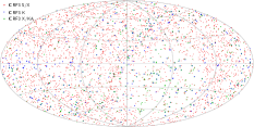
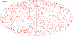
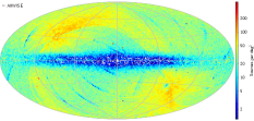
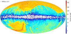
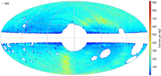
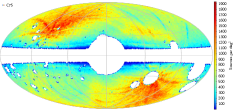
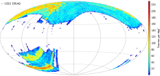
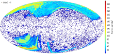
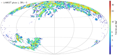
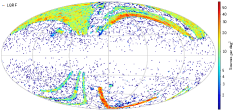
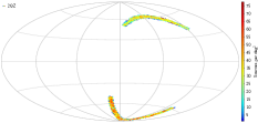
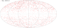
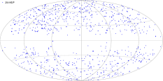
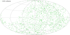
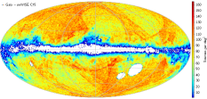
Figure 18: Distribution of the sources in the external catalogues listed in Table 1. These maps use a Hammer–Aitoff projection in galactic coordinates, with $l=b=0$ at the centre, north up, and $l$ increasing from right to left.

Appendix C Access to the Gaia-CRF3 data

Information on the Gaia-CRF3 sources is distributed over several tables in the Gaia Archive. Table gaiaedr3.agn_cross_id lists all sources (source_id) of Gaia-CRF3 together with the name of one external catalogue where the source can also be found as well as the name of the source in that catalogue. Table gaiaedr3.frame_rotator_source contains information on the sources used by the frame rotator (see Sect. 5) to define the orientation and spin of the Gaia EDR3 catalogue. Together with the Gaia EDR3 source identifier source_id, it contains the boolean flags considered_for_reference_frame_orientation and considered_for_reference_frame_spin to indicate if the source was considered by the frame rotator algorithm to fix the orientation and spin of the Gaia EDR3 catalogue, respectively. The frame rotator algorithm has a mechanism to detect outliers (see Appendix E), and another pair of boolean flags, used_for_reference_frame_orientation and used_for_reference_frame_spin, to specify which sources were used to fix, respectively, the orientation and rotation of the Gaia EDR3 catalogue. The sources that were considered but not used are the ones identified as outliers by the frame rotator algorithm.

Using these two tables and the main Gaia EDR3 astrometric table gaiaedr3.gaia_source, one can retrieve astrometric data of the Gaia-CRF3 sources and their subsets. We give here a few useful examples of ADQL queries that can be directly used in the Gaia Archive. The query

SELECT agn.source_name_in_catalogue,
       agn.catalogue_name, edr3.*
FROM gaiaedr3.agn_cross_id AS agn
INNER JOIN gaiaedr3.gaia_source AS edr3
USING (source_id)

gives a table containing astrometric data for all 1 614 173 Gaia-CRF3 sources. Adding a conditional clause at the end of the same query,

SELECT agn.source_name_in_catalogue,
       agn.catalogue_name, edr3.*
FROM gaiaedr3.agn_cross_id AS agn
INNER JOIN gaiaedr3.gaia_source AS edr3
USING (source_id)
WHERE edr3.astrometric_params_solved = 31

allows one to retrieve the astrometric data for only the 1 215 942 Gaia-CRF3 sources that have five-parameter astrometric solutions. This dataset was used for example in Gaia Collaboration et al. (2021b) to measure the acceleration of the Solar System. Changing ‘31’ to ‘95’ in the last line, one gets instead the 398 231 Gaia-CRF3 sources with six-parameter astrometric solutions.

For the sources used to define the orientation and spin of the Gaia EDR3 catalogue the following two queries are useful. The query

SELECT sub.source_name_in_catalogue,
       sub.catalogue_name, edr3.*
FROM (
SELECT frame.source_id, agn.source_name_in_catalogue,
       agn.catalogue_name
FROM gaiaedr3.frame_rotator_source AS frame
LEFT OUTER JOIN gaiaedr3.agn_cross_id AS agn
USING (source_id)
WHERE frame.used_for_reference_frame_orientation=’true’
) AS sub
INNER JOIN gaiaedr3.gaia_source AS edr3
USING (source_id)

gives data for the 2007 sources that were used to define the orientation of the Gaia EDR3 catalogue, while

SELECT sub.source_name_in_catalogue,
       sub.catalogue_name, edr3.*
FROM (
SELECT frame.source_id, agn.source_name_in_catalogue,
       agn.catalogue_name
FROM gaiaedr3.frame_rotator_source AS frame
LEFT OUTER JOIN gaiaedr3.agn_cross_id AS agn
USING (source_id)
WHERE frame.used_for_reference_frame_spin = ’true’
) AS sub
INNER JOIN gaiaedr3.gaia_source AS edr3
USING (source_id)

gives data for the 428 034 sources used to define the rotation (spin) of Gaia EDR3. The field names used_for_… can be replaced by considered_for_… to get the data of all sources considered by the reference frame algorithm. As discussed in Sect. 5, all sources that were considered by the frame rotator algorithm for fixing the orientation of the Gaia EDR3 catalogue also belong to Gaia-CRF3. However, among the sources that were considered for fixing the spin, there are 46 sources that are not part of Gaia-CRF3. Two of them were used to fix the spin. For those 46 or 2 sources, the respective queries return empty names of the source and the external catalogue.

As described in Sect. 2, the Gaia-CRF3 sources resulted from a filtered cross-match between the Gaia EDR3 catalogue and a number of external AGN/QSO catalogues. The information on which sources were found in the different external catalogues is given in table gaiadr3.gaia_crf3_xm. We note that gaiaedr3.agn_cross_id cannot be used to retrieve all Gaia-CRF3 sources from a given external catalogue, because a Gaia-CRF3 source may be found in several external catalogues but gaiaedr3.agn_cross_id only gives its identifier in one of them. To obtain a list of the Gaia-CRF3 sources that were selected from a specific external catalogue one can use the query:

SELECT xm.$$$_name, edr3.*
FROM gaiaedr3.gaia_source AS edr3
INNER JOIN gaiadr3.gaia_crf3_xm AS xm
USING (source_id)
WHERE xm.$$$ = ’true’

where ‘$$$’ should be replaced by the catalogue code from column 6 of Table 1. For the sources in the three ICRF3 catalogues (the catalogue codes icrf3sx, icrf3k, icrf3xka) gaiadr3.gaia_crf3_xm provides two source designations as also given in the original ICRF3 catalogues: the ICRF and IERS designations as icrf_name and iers_name, respectively. Additionally, the above ADQL query with the catalogue code ’b19’ can be used to see the 920 599 Gaia-CRF3 sources that were also found in the catalogue of Bailer-Jones et al. (2019).

We note that when considering an external catalogue ‘$$$’ some sources were rejected only because a lower quality of astrometry used in that catalogue resulted in the cross-match distance $\Delta$ being too large to satisfy Eq. (5) in Sect. 2. For those sources the field gaiadr3.gaia_crf3_xm.$$$ is set to false. In some cases, however, the same Gaia source was found also in other external catalogues and eventually selected for Gaia-CRF3. In those cases, the name gaiadr3.gaia_crf3_xm.$$$_name of that Gaia source in catalogue ‘$$$’ is also given. To obtain all Gaia-CRF3 sources that appear in an external catalogue one should replace the last line in the previous ADQL query by ‘WHERE xm.$$$_name IS NOT NULL’. This helps to mitigate the effect of a lower quality astrometry in some of the external catalogues and improve the overall cross-match quality for those catalogues.

Appendix D Confusion sources in Gaia EDR3

In this appendix we give the number and distributions of sources in Gaia EDR3 that satisfy Eqs. (1)–(3), ensuring that the Gaia astrometry is statistically compatible with the hypothesis that a source is extragalactic with zero parallax and proper motion. (As discussed in Sect. 2, we ignore the small effects of the Galactic acceleration and possible apparent proper motions induced by variable source structure, but take into account an overall parallax offset of $-0.017$ mas.) In this paper we call these the ‘confusion sources’, because most of them are in fact distant stars in our Galaxy or its satellite galaxies, and stellar contaminants resulting from erroneous cross-matching with external QSO catalogue (or from stellar contamination in these catalogues) can be expected to have similar characteristics as the confusion sources.

We give separate statistics for confusion sources with five- and six-parameter solutions in Gaia EDR3. For the five-parameter solutions, an explicit query of the Gaia EDR3 catalogue

SELECT * FROM gaiaedr3.gaia_source AS g
WHERE g.astrometric_params_solved = 31
  AND abs((g.parallax + 0.017)/g.parallax_error) < 5
  AND ( power(g.pmra/g.pmra_error,2)
       +power(g.pmdec/g.pmdec_error,2)
       -2*g.pmra_pmdec_corr*
          g.pmra/g.pmra_error*
          g.pmdec/g.pmdec_error)/
      (1-power(g.pmra_pmdec_corr,2)) < 25

results in 30 723 995 sources satisfying Eqs. (1)–(3). Their sky density is shown in the top panel of Fig. 19. Of those, 7 090 844 sources are in the Galactic zone with $\left|\,\sin b\,\right|<0.1$, thus violating the fourth criterion in Eq. (4). The remaining 23 633 151 confusion sources with five-parameter astrometric solutions in Gaia EDR3 satisfy all four criteria and could, based on their astrometry alone, be potential candidates for the Gaia-CRF.

A corresponding query of Gaia EDR3 for confusion sources with six-parameter solutions (obtained by changing the second line of the query to ‘WHERE g.astrometric_params_solved = 95’) returns 182 814 959 sources. Their sky density is shown in the lower panel of Fig. 19). 90 979 403 of the sources have $\left|\,\sin b\,\right|>0.1$ and thus satisfy all four criteria in Eqs. (1)–(4).

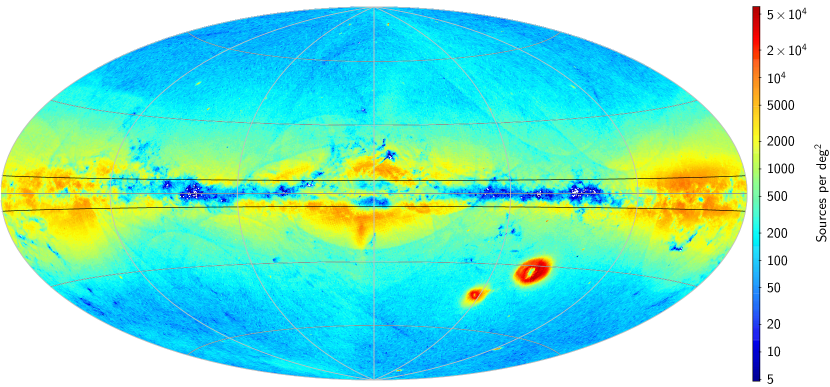
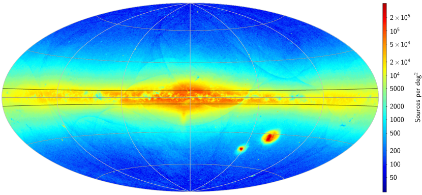
Figure 19: Distribution of the confusion sources in Gaia EDR3. These maps use a Hammer–Aitoff projection in galactic coordinates, with $l=b=0$ at the centre, north up, and $l$ increasing from right to left. The black lines bound the Galactic zone $\left|\,\sin b\,\right|<0.1$ where sources are normally excluded by Eq. (4). Top: sources with five-parameter solutions. Bottom: sources with six-parameter solutions.

Among the many features seen in Fig. 19 we recognise the expected density distribution due to the overall distribution of Galactic stars and a strong over-density in the areas of the LMC and SMC. There are several more compact high-density areas outside the Galactic plane. A detailed (but not exhaustive) inspection of the density map revealed about 20 stellar (mostly globular) clusters and 10 (dwarf) galaxies on the maps. Not counting the LMC and SMC areas, the total number of sources in these clusters and galaxies is however only about 5000, which is ignored in the statistical considerations below. We note that the Sagittarius stream is clearly visible (mainly in the top panel), as well as numerous streaks of under-density related to the scanning law.

A prominent feature in Fig. 19 is the relatively low density of sources with five-parameter solutions along the Galactic equator and in the centres of the Magellanic Clouds. This is caused by the difficulty to obtain reliable colour information from the BP and RP spectra on faint sources in these very crowded areas (Riello et al. 2021). As a result, the astrometric solution did not use a spectrophotometrically determined colour (effective wavenumber) for many of these sources, but instead determined a pseudo-colour as the sixth astrometric parameter.

Because the confusion sources in the LMC and SMC tend to have distinctly different kinematics from the Galactic stars, it is advantageous to separate out the sources in the LMC and SMC areas in the further analysis. Guided by the density maps, we take a circle of radius $9^{\circ}$ centred on $(\alpha,\delta)=(81.3^{\circ},-68.7^{\circ})$ to represent the LMC, and a circle of radius $6^{\circ}$ centred on $(\alpha,\delta)=(16.0^{\circ},-72.8^{\circ})$ to represent the SMC. These areas contain, respectively, 2 657 059 and 496 520 confusion sources with five-parameter solutions (6 817 915 and 1 307 591 with six-parameter solutions). This simplistic selection does not pretend to any deeper physical significance, and only partially coincides with the carefully selected samples of Gaia EDR3 sources in the LMC and SMC discussed in Gaia Collaboration et al. (2021c).

Figure 20 shows the distribution of the confusion sources in galactic coordinates and magnitude, split by the kind of solution (five or six parameters) and further divided into four disjoint groups: sources in the LMC and SMC areas defined above, and for the remaining sources according to $\left|\,\sin b\,\right|\gtrless 0.1$. The confusion sources outside the LMC and SMC areas are called ‘Galactic’ below, although it is clear that this set contains also many extragalactic objects.

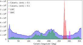
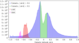
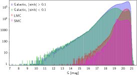
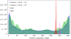
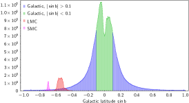
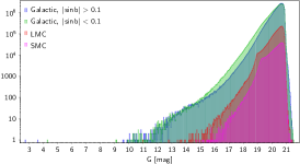
Figure 20: Distribution of confusion sources in (from left to right) galactic longitude, sine of galactic latitude, and magnitude. Top: sources with five-parameter solutions. Bottom: sources with six-parameter solutions. The selections indicated in the legend are further explained in the text.

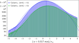
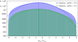
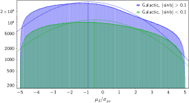
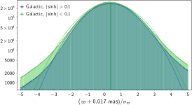
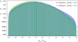
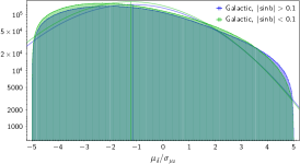
Figure 21: Histograms of the normalised parallaxes and proper motion components for the Galactic confusion sources. Top: sources with five-parameter solutions. Bottom: sources with six-parameter solutions. The different colours show the selections indicated in the legend.

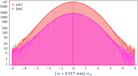
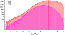
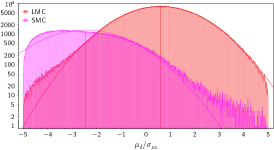
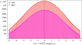
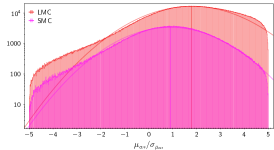
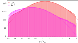
Figure 22: Histograms of the normalised parallaxes and proper motion components for the confusion sources in the LMC and SMC areas. Top: sources with five-parameter solutions. Bottom: sources with six-parameter solutions.

Figures 21 and 22 show the distributions of the normalised parallaxes and proper motions of the confusion sources separately for the Galactic sources (split by galactic latitude) and the LMC and SMC areas. The distributions are strongly non-Gaussian (with the possible exception of parallaxes in the LMC/SMC areas) and very different from those of the Gaia-CRF3 sources in Fig. 3. In Sect. 2, this difference was used to check the purity of the filtered sources in the external QSO catalogues and in the final Gaia-CRF3. The proper motions give the strongest indication of impurity. Interestingly, for the Galactic confusion sources there is no clear dependence according to $\left|\,\sin b\,\right|\gtrless 0.1$. On the other hand, the confusion sources in the LMC and SMC areas give rather different and distinct distributions. The distributions for the five- and six-parameter solutions are not drastically different and mainly reflect the generally higher uncertainties of the six-parameter sources, which makes their distributions slightly less non-Gaussian.

Selection of QSO-like objects in the Gaia catalogue, based exclusively on parallaxes and proper motions, is an interesting prospect already discussed in the literature (Heintz et al. 2015; 2018). Among the Gaia EDR3 sources with five-parameter solutions, there are 23.6 million satisfying Eqs. (1)–(4), of which 1.2 million (5.1%) are also in Gaia-CRF3. Allowing that the actual number of QSOs among the five-parameter sources in Gaia EDR3 could be a factor two higher (cf. Sect. 3), we conclude that the purity of such a selection from Gaia EDR3 would be at most about 10% – too low to be of practical use, but still interesting and promising. In certain areas on the sky the percentage of true QSO-like sources in the sample is much higher. For example, excluding $\left|\,b\,\right|<20^{\circ}$ and the LMC/SMC areas, there are 5 767 163 confusion sources, of which 1 410 314 (24.5%) are Gaia-CRF3 sources. The purity of such selections in future Gaia data releases will improve drastically thanks to the higher accuracy of parallaxes and (especially) proper motions (cf. Sect. 2.5).

Appendix E Estimating the spin and orientation corrections

As described in Sect. 6.1 of Lindegren et al. (2012), the frame rotator is an integral part of AGIS with three main functions: (i) to estimate the spin and orientation corrections needed to bring the current astrometric solution onto the ICRS; (ii) to apply the estimated corrections to the astrometric parameters of the primary sources; and (iii) to apply the corresponding corrections to the attitude parameters. This appendix describes the algorithm used for the first function in the construction of Gaia EDR3.

The 2012 paper gave a stringent mathematical framework for all three functions and outlined how they could be implemented in AGIS. The frame rotator used for the first two releases of Gaia data followed these prescriptions quite rigorously, which however resulted in code that was unnecessarily complex and not very transparent. For example, it permitted the use of different reference epochs for the AGIS solution, comparison catalogue, and orientation parameters, while in practice this was never needed. It also foresaw the use of radio stars observed by VLBI to help align the reference frame, which is no longer considered necessary or even desirable. On the other hand, the details of the numerical algorithm used for the robust least-squares estimation (LSE) of the rotation parameters were not at all described in Lindegren et al. (2012), making it very difficult for outside users to reproduce how the frame rotator worked in those releases.

In 2018 it was decided to implement a new version of the frame rotator to be used for the third and subsequent data releases. The main changes with respect to the earlier version are as follows: only two kinds of sources are used for estimating the rotation parameters, namely QSO-like sources with high-accuracy external positions (the VLBI positions of ICRF3 S/X in Gaia EDR3), used for both orientation and spin, and QSO-like sources without accurate external positions, used only for the spin. The same reference epoch is used for rotation parameters as for the astrometric data (2016.0 for (E)DR3), which permits to separate completely the solution for the orientation from that of the spin. Furthermore, the observation equations are written directly in terms of the proper motions and position differences (Sect. E.1), rather than using the rigorous but less transparent formalism of Lindegren et al. (2012). The solution takes into account the correlation between the components in right ascension and declination of both Gaia and external data (Sect. E.2), and has a transparent scheme for the detection and treatment of outliers (Sect. E.3). Finally, the solution provides reasonable estimates of the statistical uncertainties of the rotation parameters also when the uncertainties of the input data are underestimated (Sect. E.4), and may optionally include additional terms, such as a glide in the proper motions or more general expansions of the proper motions and position differences (Sect. E.5).

All these changes concern the estimation algorithm, that is the first function of the frame rotator. The remaining two functions, that is the application of the corrections to the source and attitude data, are still done as described in Sects. 6.1.2 and 6.1.3 of the 2012 paper and are not further discussed here.

We denote by ${\cal Q}_{0}$ the set of QSO-like sources considered for the determination of the spin correction, of which the subset ${\cal Q}$ was actually used after elimination of outliers; similarly, ${\cal R}_{0}$ and ${\cal R}$ are the set of sources considered and used for the determination of the orientation. Although not required by the algorithm, we normally have ${\cal R}_{0}\subseteq{\cal Q}_{0}$. The number of sources in each set is denoted $n({\cal Q}_{0})$, etc. We use $\sigma(x)$, $\rho(x,y)$, and $\text{Cov}(x,y)$ for the uncertainty, correlation coefficient, and covariance of the arbitrary parameters $x$ and $y$. The asterisk in $\alpha^{*}$ indicates that the $\cos\delta$ factor is implicit, as in $\mu_{\alpha^{*}}=\dot{\alpha}\cos\delta$. To distinguish between data in the current astrometric solution and the corresponding data in the external catalogue, we put an overline ($\bar{\phantom{x}}$) on the latter. The prime ^′ denotes the matrix transpose.

E.1 Observation equations

Let $\mbox{\boldmath$\omega$}=[\omega_{X},\leavevmode\nobreak\ \omega_{Y},\leavevmode\nobreak\ \omega_{Z}]^{\prime}$ be the spin correction of the current solution, expressed by its components along the principal axes of the ICRS. (As indicated by the prime, $\omega$ is a column matrix.) In matrix form, the observation equations in proper motion for source $i$ are

$$\mbox{\boldmath$A$}_{i}\mbox{\boldmath$\omega$}=\mbox{\boldmath$\mu$}_{i}\,,$$ (14)

with coefficient matrix

$$\mbox{\boldmath$A$}=\begin{bmatrix}-\cos\alpha_{i}\sin\delta_{i}&\quad&+\sin\alpha_{i}\sin\delta_{i}&\quad&+\cos\delta_{i}\\ +\sin\alpha_{i}&&-\cos\alpha_{i}&&0\end{bmatrix}\,$$ (15)

and right-hand side

$$\mbox{\boldmath$\mu$}_{i}=\begin{bmatrix}\mu_{\alpha^{*}i}\\ \mu_{\delta{}i}\end{bmatrix}\,.$$ (16)

Here, $\alpha_{i}$, $\delta_{i}$, $\mu_{\alpha^{*}i}$ and $\mu_{\delta{}i}$ are the position and proper motion components of the source in the current solution, with reference epoch $t_{\text{ref}}$ ($=2016.0$ for Gaia EDR3). For the weight normalisation and decorrelation (Sect. E.2), we also need the covariance of the right-hand side in Eq. (16),

$$\text{Cov}(\mbox{\boldmath$\mu$}_{i})=\\ \begin{bmatrix}\sigma(\mu_{\alpha^{*}i})^{2}&\rho(\mu_{\alpha^{*}i},\mu_{\delta{}i})\,\sigma(\mu_{\alpha^{*}i})\,\sigma(\mu_{\delta{}i})\leavevmode\nobreak\ \\[6.0pt] \leavevmode\nobreak\ \rho(\mu_{\alpha^{*}i},\mu_{\delta{}i})\,\sigma(\mu_{\alpha^{*}i})\,\sigma(\mu_{\delta{}i})&\sigma(\mu_{\delta{}i})^{2}\end{bmatrix}\,.$$ (17)

Similarly, let $\mbox{\boldmath$\varepsilon$}=[\varepsilon_{X},\leavevmode\nobreak\ \varepsilon_{Y},\leavevmode\nobreak\ \varepsilon_{Z}]^{\prime}$ be the orientation correction at the reference epoch $t_{\text{ref}}$, expressed by its components in the ICRS. The linearised observation equations in position for source $i$ are

$$\mbox{\boldmath$A$}_{i}\mbox{\boldmath$\varepsilon$}=\mbox{\boldmath$\Delta$}_{i}\,,$$ (18)

with the same coefficient matrix $\mbox{\boldmath$A$}_{i}$ as before. The right-hand side,

$$\mbox{\boldmath$\Delta$}_{i}\equiv\begin{bmatrix}\Delta\alpha^{*}_{i}\\ \Delta\delta_{i}\end{bmatrix}=\begin{bmatrix}\left(\alpha_{i}-\bar{\alpha}_{i}\right)\cos\delta_{i}\\ \delta_{i}-\bar{\delta}_{i}\end{bmatrix}\,,$$ (19)

is the difference between the position $(\alpha_{i},\leavevmode\nobreak\ \delta_{i})$ in the current solution and the position $(\bar{\alpha}_{i},\leavevmode\nobreak\ \bar{\delta}_{i})$ according to the external catalogue. We note that the external positions at $t_{\text{ref}}$ (= 2016.0 for EDR3) should be used here. In particular, for Gaia EDR3 the galactic acceleration should be taken into account with the ICRF3 S/X positions as prescribed in Sect. 5.3 of Charlot et al. (2020). The covariance of $\mbox{\boldmath$\Delta$}_{i}$ in Eq. (19) is computed on the assumption that the positional errors of the current solution and of the external catalogue are independent:

$$\text{Cov}(\mbox{\boldmath$\Delta$}_{i})=\text{Cov}(\alpha^{*}_{i},\leavevmode\nobreak\ \delta_{i})+\text{Cov}(\bar{\alpha}^{*}_{i},\leavevmode\nobreak\ \bar{\delta}_{i})\,,$$ (20)

where

$$\text{Cov}(\alpha^{*}_{i},\leavevmode\nobreak\ \delta_{i})=\\ \begin{bmatrix}\sigma(\alpha^{*}_{i})^{2}&\quad&\rho(\alpha^{*}_{i},\delta_{i})\,\sigma(\alpha^{*}_{i})\,\sigma(\delta_{i})\leavevmode\nobreak\ \\[6.0pt] \leavevmode\nobreak\ \rho(\alpha^{*}_{i},\delta_{i})\,\sigma(\alpha^{*}_{i})\,\sigma(\delta_{i})&\quad&\sigma(\delta_{i})^{2}\end{bmatrix}\,,$$ (21)

and correspondingly for the external data. We note that

$$\sigma(\Delta\alpha^{*}_{i}) =\sqrt{\sigma(\alpha^{*}_{i})^{2}+\sigma(\bar{\alpha}^{*}_{i})^{2}}\,,$$ (22)

$$\sigma(\Delta\delta_{i}) =\sqrt{\sigma(\delta_{i})^{2}+\sigma(\bar{\delta}_{i})^{2}}\,,$$ (23)

$$\rho(\Delta\alpha^{*}_{i},\Delta\delta_{i}) =\frac{\rho(\alpha^{*}_{i},\delta_{i})\,\sigma(\alpha^{*}_{i})\,\sigma(\delta_{i})+\rho(\bar{\alpha}^{*}_{i},\bar{\delta}_{i})\,\sigma(\bar{\alpha}^{*}_{i})\,\sigma(\bar{\delta}_{i})}{\sigma(\Delta\alpha^{*}_{i})\,\sigma(\Delta\delta_{i})}\,.$$ (24)

The total number of observation equations considered for $\omega$ is $2n({\cal Q}_{0})$, and for $\varepsilon$ it is $2n({\cal R}_{0})$. A feature of the algorithm described here is that the observation equations always come in pairs, as in Eqs. (14) and (18), and that the two components in a pair are always treated together. This simplifies the decorrelation of data (see below), and affects the way outliers are detected and removed. The resulting solution and statistics are independent of the coordinate system in which they are calculated.

E.2 Weight normalisation and decorrelation

Because the observation equations have different uncertainties (heteroscedasticity) and are pairwise correlated, they should be solved by the generalised least-squares method for optimality. Equivalently, the ordinary (unweighted) least-squares method can be applied to the normalised equations,

$$\mbox{\boldmath$K$}_{i}\mbox{\boldmath$A$}_{i}\mbox{\boldmath$\omega$} =\mbox{\boldmath$K$}_{i}\mbox{\boldmath$\mu$}_{i}\,,$$ (25)

$$\mbox{\boldmath$L$}_{i}\mbox{\boldmath$A$}_{i}\mbox{\boldmath$\varepsilon$} =\mbox{\boldmath$L$}_{i}\mbox{\boldmath$\Delta$}_{i}\,,$$ (26)

where $\mbox{\boldmath$K$}_{i}$ and $\mbox{\boldmath$L$}_{i}$ are $2\times 2$ matrices chosen in such a way that the transformed right-hand sides are uncorrelated and of unit variance. This condition does not define $\mbox{\boldmath$K$}_{i}$ and $\mbox{\boldmath$L$}_{i}$ uniquely, since any orthogonal transformation of them will give the same result; the form used here is the inverse lower Cholesky factor of the covariance matrix, or

$$\mbox{\boldmath$K$}_{i}=\begin{bmatrix}\frac{1}{\sigma(\mu_{\alpha^{*}i})}&\quad&0\\[12.0pt] \leavevmode\nobreak\ \frac{-\rho(\mu_{\alpha^{*}i},\,\mu_{\delta{}i})}{\sigma(\mu_{\alpha^{*}i})\sqrt{1-\rho(\mu_{\alpha^{*}i},\,\mu_{\delta{}i})^{2}}}&\quad&\frac{1}{\sigma(\mu_{\delta{}i})\sqrt{1-\rho(\mu_{\alpha^{*}i},\,\mu_{\delta{}i})^{2}}}\leavevmode\nobreak\ \end{bmatrix}\,$$ (27)

and

$$\mbox{\boldmath$L$}_{i}=\begin{bmatrix}\frac{1}{\sigma(\Delta\alpha^{*}_{i})}&\quad&0\\[12.0pt] \leavevmode\nobreak\ \frac{-\rho(\Delta\alpha^{*}_{i},\,\Delta\delta_{i})}{\sigma(\Delta\alpha^{*}_{i})\sqrt{1-\rho(\Delta\alpha^{*}_{i},\,\Delta\delta_{i})^{2}}}&\quad&\frac{1}{\sigma(\Delta\delta_{i})\sqrt{1-\rho(\Delta\alpha^{*}_{i},\,\Delta\delta_{i})^{2}}}\leavevmode\nobreak\ \end{bmatrix}\,.$$ (28)

It is readily verified that, as required, $\mbox{\boldmath$K$}_{i}\text{Cov}(\mbox{\boldmath$\mu$}_{i})\mbox{\boldmath$K$}_{i}{{}^{\prime}}=\mbox{\boldmath$I$}$ and $\mbox{\boldmath$L$}_{i}\text{Cov}(\mbox{\boldmath$\Delta$}_{i})\mbox{\boldmath$L$}_{i}{{}^{\prime}}=\mbox{\boldmath$I$}$, where $I$ is the identity matrix.

Given the subsets ${\cal Q}$, ${\cal R}$ of the accepted sources, the generalised least-squares solutions are obtained by minimising the sum of squared normalised residuals,

$$X^{2}(\mbox{\boldmath$\omega$},{\cal Q}) =\sum_{i\,\in\,{\cal Q}}\,\bigl{|}\mbox{\boldmath$K$}_{i}\mbox{\boldmath$\mu$}_{i}-\mbox{\boldmath$K$}_{i}\mbox{\boldmath$A$}_{i}\mbox{\boldmath$\omega$}\,\bigr{|}^{2}\,,$$ (29)

$$X^{2}(\mbox{\boldmath$\varepsilon$},{\cal R}) =\sum_{i\,\in\,{\cal R}}\,\bigl{|}\mbox{\boldmath$L$}_{i}\mbox{\boldmath$\Delta$}_{i}-\mbox{\boldmath$L$}_{i}\mbox{\boldmath$A$}_{i}\mbox{\boldmath$\varepsilon$}\,\bigr{|}^{2}\,.$$ (30)

This can be done by a range of standard numerical techniques, including orthogonal transformations and the use of normal equations (e.g. Lawson & Hanson 1995, Björck 1996). For the frame rotator, the normalised observation equations in Eqs. (25) and (26) are solved by QR decomposition, using Householder transformations.

E.3 Residual statistics and treatment of outliers

Standard least-squares fitting is sensitive to outliers, that is data points that do not reasonably fit the observation equations, considering the uncertainties and the typical scatter of residuals. Outliers must be expected among the external counterparts, as well as among the other QSO-like sources, for a variety of reasons. It is therefore essential that the fit is robust against outliers. The method adopted for the frame rotator is to identify the outliers that must be removed from the originally considered samples (${\cal Q}_{0}$, ${\cal R}_{0}$) to create the subsets ${\cal R}$ and ${\cal Q}$ used in Eqs. (30) and (29). Two things should be noted concerning this process. Firstly, outliers are identified at source level, that is, a given source is either rejected in both coordinates ($\alpha$ and $\delta$, or $\mu_{\alpha^{*}}$ and $\mu_{\delta}$), or accepted in both coordinates. This makes sense from a physical viewpoint, because a ‘bad’ source is probably bad (at some level) in both coordinates. Secondly, because $\omega$ and $\varepsilon$ are treated separately, it happens that a source rejected in ${\cal R}$ (for the orientation) is accepted in ${\cal Q}$ (for the spin), or vice versa. Again, this could be motivated on physical grounds.

Details of the subsequent algorithm are exactly the same for Eqs. (29) and (30), and are therefore described in terms of the generic function

$$X^{2}(\mbox{\boldmath$x$},{\cal S})=\sum_{i\,\in\,{\cal S}}\,X^{2}_{i}(\mbox{\boldmath$x$})\,,$$ (31)

where

$$X_{i}(\mbox{\boldmath$x$})=\bigl{|}\,\mbox{\boldmath$d$}_{i}-\mbox{\boldmath$D$}_{i}\mbox{\boldmath$x$}\,\bigr{|}\,.$$ (32)

Here, $x$ could be either $\omega$ or $\varepsilon$, with ${\cal S}$, $d$, and $D$ correspondingly defined according to Eq. (29) or (30).

We note that the functions $X_{i}(\mbox{\boldmath$x$})$, which can be computed for all the sources in ${\cal S}_{0}$, are a natural measure of the discrepancy of source $i$ from the model for given parameter vector $x$. A useful overall statistic is the median discrepancy

$$X_{0.5}(\mbox{\boldmath$x$})=\operatorname*{med\,}_{i\,\in\,{\cal S}_{0}}\bigl{(}X_{i}(\mbox{\boldmath$x$})\bigr{)}\,,$$ (33)

and a robust estimator could be to simply minimise this quantity. However, if the errors are approximately Gaussian, with a moderate fraction of outliers, robust least-squares estimation is more accurate and therefore preferred for the frame rotator. If $x$ is the true parameter vector, and all the errors are Gaussian with nominal covariances, $X_{0.5}(\mbox{\boldmath$x$})$ is expected to be around $\sqrt{\ln 4}\simeq 1.1774$ (which is the median of the chi-distribution with two degrees of freedom).

The adopted solution $\hat{x}$ and accepted subset ${\cal S}$ simultaneously satisfy the three conditions

$$\left.\begin{aligned} \mbox{\boldmath$\hat{x}$}=\operatorname*{argmin}_{\mbox{\boldmath$x$}}\sum_{i\,\in\,{\cal S}}X^{2}_{i}(\mbox{\boldmath$x$})\,,\\ \forall i\in{\cal S}:X_{i}(\mbox{\boldmath$\hat{x}$})\leq\kappa\,X_{0.5}(\mbox{\boldmath$\hat{x}$})\,,\\[6.0pt] \forall i\in{\cal S}_{0}\backslash{\cal S}:X_{i}(\mbox{\boldmath$\hat{x}$})>\kappa\,X_{0.5}(\mbox{\boldmath$\hat{x}$})\,\end{aligned}\quad\right\}$$ (34)

for the chosen clip limit $\kappa\geq 1$ (see below). It is not obvious that these conditions lead to a unique solution; indeed, it is easy to construct examples where this is not the case, for example if ${\cal S}_{0}$ consists of disjoint subsets with distinctly different rotation parameters. However, these are somewhat contrived examples and in practice the non-uniqueness is hardly an issue. More relevant is the question whether a solution always exists – to which we do not know the answer. We take the pragmatic view that a unique solution ‘close enough’ to satisfying Eq. (34) can always be found by the following algorithm.

Start by provisionally accepting all the sources in ${\cal S}_{0}$, compute the least-squares estimate $\mbox{\boldmath$\hat{x}$}_{0}$ by minimising $X^{2}(\mbox{\boldmath$x$},{\cal S}_{0})$, and hence obtain the statistic $X_{0.5}(\mbox{\boldmath$\hat{x}$}_{0})$. In the next iteration, let ${\cal S}_{1}$ be the subset of sources satisfying $X_{i}(\mbox{\boldmath$\hat{x}$}_{0})\leq\kappa\,X_{0.5}(\mbox{\boldmath$\hat{x}$}_{0})$, leading to the estimate $\mbox{\boldmath$\hat{x}$}_{1}$ minimising $X^{2}(\mbox{\boldmath$x$},{\cal S}_{1})$ and the new statistic $X_{0.5}(\mbox{\boldmath$\hat{x}$}_{1})$, from which the subset ${\cal S}_{2}$ is constructed, and so on. This gives a sequence of subsets ${\cal S}_{k}$, $k=0,\,1,\,2,\,\dots$ that may converge to a stable subset (i.e. ${\cal S}_{k+1}={\cal S}_{k}$ for some $k$). If so, the stable subset and the corresponding estimate $\mbox{\boldmath$\hat{x}$}_{k}$ is the desired solution. But even if the sequence does not converge, it will sooner or later be found that the same subsets reappear cyclically in the sequence, that is ${\cal S}_{k+p}={\cal S}_{k}$, where $p>1$ is the cycle period. In such a case any of the solutions in the cycle might be accepted. However, by adopting the rule that the sequence is stopped at the lowest $k$ where ${\cal S}_{k}={\cal S}_{k-p}$ for some $p>0$, we arrive at a unique result both for a converging sequence ($p=1$) and in the cyclic case ($p>1$).

To avoid having to save and compare the (potentially many and large) subsets ${\cal S}_{k}$, we assign a fixed random number $r_{i}$ to each source in ${\cal S}_{0}$, and save from previous iterations only the outlier ‘checksum’ $o_{k}=\sum_{i\,\in\,{\cal S}_{0}\backslash{\cal S}_{k}}r_{i}$. The iteration stops as soon as $o_{k}=o_{k-p}$ for some $p>0$, at which point we adopt ${\cal S}={\cal S}_{k}$ and $\mbox{\boldmath$\hat{x}$}=\mbox{\boldmath$\hat{x}$}_{k}$ as the solution.

The clip limit $\kappa$ is a dimensionless number, typically in the range 2–5, to be chosen by the researcher. A value $\kappa\geq 1$ ensures that at most 50% of the sources in ${\cal S}_{0}$ are rejected as outliers, but in practice a higher value should always be used. In principle, an optimum clip level that minimises the expected uncertainty of $\hat{x}$ can be estimated by careful modelling of the actual error distribution in ${\cal S}_{0}$, but for the frame rotator we always use a fixed $\kappa=3$. In the nominal case of purely Gaussian errors and no actually bad data, this will (erroneously) reject about 1% of the sources. This appears to be an acceptable price to pay for an estimation algorithm that is both efficient and very robust.

E.4 Uncertainty of the estimates

The covariance of $\hat{x}$ is estimated as

$$\text{Cov}\left(\mbox{\boldmath$\hat{x}$}\right)=\left[\sum_{i\,\in\,{\cal S}}\mbox{\boldmath$D$}_{i}^{\prime}\mbox{\boldmath$D$}_{i}\right]^{-1}\times f\,,$$ (35)

where the first factor (the inverse of the weighted normal matrix) is the nominal covariance obtained on the assumption that the data uncertainties in $\text{Cov}(\mbox{\boldmath$\Delta$}_{i})$ and $\text{Cov}(\mbox{\boldmath$\mu$}_{i})$ are correctly estimated, and that no outlier rejection is applied. An empirical correction factor $f>0$ takes into account that the data uncertainties may be systematically wrong (usually underestimated), and that the nominal covariance estimate is biased by the outlier rejection process even if the data uncertainties are correctly estimated.

In practice, the correction factor $f$ must be derived from the residuals of the least-squares solution, or in our case from the statistics of $X_{i}(\mbox{\boldmath$\hat{x}$})$. An obvious possibility is to use the reduced chi-square (the square of the unit weight error $u$),

$$u^{2}=\frac{X^{2}(\mbox{\boldmath$\hat{x}$},{\cal S})}{2n({\cal S})-m}\,,$$ (36)

as an estimate of $f$, where $n({\cal S})$ is the number of accepted sources and $m$ is the dimension of $x$ (here, $m=3$). This is accurate if $n({\cal S})$ is large (as it usually is in our applications), the fraction of outliers is very small, and the data uncertainties are biased by an approximately constant factor. However, when a significant fraction of the sources are rejected as outliers, the use of $f=u^{2}$ tends to severely underestimate the uncertainties of $\hat{x}$. A more reasonable correction factor should therefore consider the error distribution in the full sample ${\cal S}_{0}$, not just in the accepted subset ${\cal S}$. Discrepancy quantiles such as $X_{0.5}$ in Eq. (33) provide robust characterisation of the full error distribution.

Based on numerical simulations, we have adopted the following recipe for the correction factor to be used in Eq. (35):

$$f=\max\left[u^{2},\leavevmode\nobreak\ X^{2}_{0.5}/(\ln 4)\right]\,.$$ (37)

In the ideal case of Gaussian errors, correctly estimated data uncertainties, and a negligible fraction of outliers, we expect $u^{2}\simeq 1$ and $X^{2}_{0.5}\simeq\ln 4$, and hence $f\simeq 1$. If the data uncertainties are biased by a certain factor, both $u$ and $X_{0.5}$ scale by the same factor, and the recipe still works. For samples yielding a non-negligible fraction of outliers we normally have $u^{2}<X^{2}_{0.5}/(\ln 4)$, and the higher factor then tends to give a more accurate estimate of the uncertainties, hence Eq. (37).

E.5 Optional parameters

The estimation as described above has only three unknowns, that is the components of $\omega$ or $\varepsilon$. The algorithm, including weight normalisation, decorrelation, and outlier treatment, is readily adapted to more general linear models, for example using VSH to represent higher-order distortions of the proper motions and position differences (Mignard & Klioner 2012), or including terms depending on the colour and magnitude of the source. However, while such more complex models are useful for investigating the properties of the final catalogue, they should normally not be used in the frame rotator.

One possible exception is the glide in proper motion, which is expected to be present on physical grounds. Already in Gaia EDR3 this effect is very clear, and found to be consistent with the expected Galactic acceleration of the solar system barycentre (Gaia Collaboration et al. 2021b). The proper motion model implicit in Eq. (14) neglects this effect, which was deemed acceptable for the frame rotator in the first three releases of Gaia astrometry. For future releases this may not be accurate enough (since the effects of rotation and glide can be correlated and mutually disturb each other). One possible remedy is then to correct the observed proper motions in Eq. (16) for the assumed Galactic glide. However, a better option may be to estimate the glide $g$ together with $\omega$, using the augmented observation equations

$$\mbox{\boldmath$A$}_{i}\mbox{\boldmath$\omega$}+\mbox{\boldmath$B$}_{i}\mbox{\boldmath$g$}=\mbox{\boldmath$\mu$}_{i}\,.$$ (38)

The estimation follows the generic scheme outlined above, minimising $X^{2}=\sum_{i\,\in\,{\cal Q}}\,|\,\mbox{\boldmath$d$}_{i}-\mbox{\boldmath$D$}_{i}\mbox{\boldmath$x$}\,|^{2}$ with

$$\mbox{\boldmath$x$}=\begin{bmatrix}\mbox{\boldmath$\omega$}\\ \mbox{\boldmath$g$}\end{bmatrix}\,,\quad\mbox{\boldmath$d$}_{i}=\mbox{\boldmath$L$}_{i}\mbox{\boldmath$\mu$}_{i}\,,\quad\text{and}\quad\mbox{\boldmath$D$}_{i}=\mbox{\boldmath$L$}_{i}\,\Bigl{[}\,\mbox{\boldmath$A$}_{i}\leavevmode\nobreak\ \leavevmode\nobreak\ \mbox{\boldmath$B$}_{i}\,\Bigr{]}\,.$$ (39)

It should be noted that the application of the spin and orientation corrections to the source and attitude data, that is functions (ii) and (iii) of the frame rotator, is in any case restricted to the pure rotations given by $\omega$ and $\varepsilon$. In particular, the published source parameters are never corrected for the (assumed or estimated) glide in proper motion.