Learning Eco-Driving Strategies at Signalized Intersections

Abstract

Signalized intersections in arterial roads result in persistent vehicle idling and excess accelerations, contributing to fuel consumption and CO₂ emissions. There has thus been a line of work studying eco-driving control strategies to reduce fuel consumption and emission levels at intersections. However, methods to devise effective control strategies across a variety of traffic settings remain elusive. In this paper, we propose a reinforcement learning (RL) approach to learn effective eco-driving control strategies. We analyze the potential impact of a learned strategy on fuel consumption, CO₂ emission, and travel time and compare with naturalistic driving and model-based baselines. We further demonstrate the generalizability of the learned policies under mixed traffic scenarios. Simulation results indicate that scenarios with 100% penetration of connected autonomous vehicles (CAV) may yield as high as 18% reduction in fuel consumption and 25% reduction in CO₂ emission levels while even improving travel speed by 20%. Furthermore, results indicate that even 25% CAV penetration can bring at least 50% of the total fuel and emission reduction benefits.

I Introduction

Global greenhouse gas emission and fuel consumption rates have significantly increased over the last decade, indicating early signs of a major climate crisis in the near future. While many sectors actively contribute to greenhouse gas emission (GHG), transportation sector in the US contributes 29% of which 77% is due to land transportation [1]. With clear indications that frequent vehicle stops created by stop-and-go waves [2, 3], slow speeds on congested roads, over speeds [3, 4], and idling can significantly increase fuel consumption and emission levels, carefully designed driving strategies are becoming imperative. The urge to reduce fuel consumption and related emission levels in driving has thus created a line of work on studying eco-driving strategies.

In particular, eco-driving at signalized intersections has received significant attention due to the possible energy savings and reduction of emission levels. In arterial roads, traffic signals result in stop-and-go traffic waves producing acceleration, and idling events, increasing fuel consumption and emission levels. Recent studies have thus utilized connected automated vehicles (CAVs) as a means of control to achieve low fuel consumption and emissions when approaching and leaving an intersection [5]. Such CAV control techniques fall under the broad umbrella of Lagrangian control, which describes traffic control techniques based on mobile actuators (e.g. vehicles), rather than fixed-location actuators (e.g. traffic signals). In addition, the capability of CAVs to sense or communicate with nearby vehicles using V2V (Vehicle to Vehicle) and nearby intersections to exchange Signal and Phase Timing (SPaT) messages through V2I (Vehicle to Infrastructure) makes them well-suited control units for the Lagrangian control.

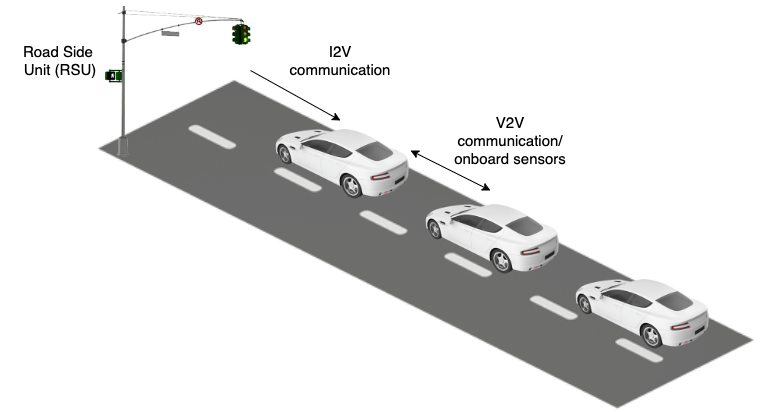
Figure 1: Schematic overview of the approaching fleet of CAVs in a signalized intersection and the communication channels available for eco-driving

Most of the existing work on energy efficient driving at signalized intersections make assumptions on the vehicle dynamics and inter-vehicle dynamics, simplify the objective only to reduce fuel/emission without considering the impact on travel time, or usually involve solving a non-linear optimization problem in real time [5, 6, 7]. Such methods fall under the broader class of model-based control methods.

Recently, learning-based model-free control methods have been proposed to solve challenging control problems. In particular, deep reinforcement learning has been used in obtaining desired control policies in many control tasks ranging from transportation [8, 9], and healthcare [10] to economics and finance [11]. In this work, we leverage deep reinforcement learning (DRL) to obtain Lagrangian control policies for CAVs when approaching and leaving a signalized intersection. In particular, we take a multi-agent DRL approach.

Unlike most existing works, which focus on reducing fuel consumption or emission reduction without explicitly factoring in the impact on travel time caused by the new strategy, we formulate a more realistic objective by reducing fuel consumption while minimizing the impact on travel time. Since there is a general consensus that the fuel consumption is proportional to CO₂ emission levels [12], we also measure CO₂ emission levels under the resultant policy.

We show that the learned control policies perform on par with model-based baselines and significantly outperform naturalistic driving baselines, and the transfer capacity to out-of-distribution settings is successful.

Our main contributions in this study are:

• We formulate Lagrangian control at intersections as a Partially Observable Markov Decision Process (POMDP) and solve it using reinforcement learning to reduce fuel consumption (and thereby emission levels) caused by accelerations, and idling while minimizing the impact on travel time.

• We assess the benefit of learned eco-driving control policies under naturalistic driving scenarios and model-based baselines and show significant savings in fuel and reductions in emission levels even while improving the average travel time.

• We assess the generalizability of the learned policies by zero-shot transfer of the learned control policies to mixed traffic scenarios (varying CAV penetration rates) that were unseen at the training time.

II Related Work

II-A Eco-driving

Studies on eco-driving can be categorized into freeway-based and arterial-based control strategies. Freeway-based strategies are mainly concerned with maintaining a desirable speed without fluctuations, as traffic flow is rarely affected by traffic signals. This is usually achieved using advisory speed limits [13] or platoon-based operations [14]. Arterial-based eco-driving is more involved due to the shock waves created by consecutive traffic signals. Yang et al. and Yang et al. introduce eco-driving control strategies based on queue length estimates and queue discharging estimates for single and multiple intersections, respectively [15, 5]. Ozkan et al. propose a receding-horizon optimization-based non-linear model predictive control algorithm for CAVs to reduce fuel consumption [7]. Zhao et al. propose a platoon-based eco-driving strategy for mixed traffic [16]. Similarly, model predictive control (MPC) is employed in HomChaudhuri et al. [17] where as dynamic programming is used in Sun et al. [18].

Additionally, there have been experimental field studies that focus on eco-driving. Many of them study the benefit of eco-driving that arises from smart driving after a fuel-efficient driving course was provided to a selected set of human drivers [19, 20]. Further studies have also been carried out to field test and quantify the fuel saving benefits of eco-driving using CAVs [21, 22].

However, all these work share a standard set of limitations. They usually assume a model of the dynamics, require solving a non-linear optimization problem in real-time, are not amenable to changes in the environments or make assumptions on queue lengths around the signalized intersection and the respective discharging rates. In contrast, our proposed DRL method does not assume any model of the dynamics, is faster to execute, and makes no assumptions of the queue length or discharging rates.

II-B Reinforcement learning for autonomous traffic control

Reinforcement learning has been gaining notable attention recently due to its ability to learn near-optimal control in complex environments. Many recent studies have attempted to use RL in devising control strategies in various traffic tasks. Wu et al. demonstrated the use of RL in mixed traffic scenarios and showed even a fraction of autonomous vehicles could stabilize the traffic from stop-and-go waves [9]. Vinitsky et al. use RL to derive Lagrangian control policies for autonomous vehicles to improve the throughput of a bottleneck [23]. Yan et al. [24] demonstrated that even without reward shaping, reinforcement learning based CAVs learn to coordinate to exhibit traffic signal-like behaviors [24]. Many studies have utilized RL in traffic signal control and have shown significant benefits that are otherwise hard to obtain [25, 26].

Recently a few works have utilized RL to derive eco-driving control strategies. Zhu et al. use RL to seek optimal speed and power profiles to minimize fuel consumption over a given trip itinerary [27] for a single CAV. Similar work has been done by Guo et al. with an auxiliary model to factor in lane changing [28]. Wegner et al. propose a twin-delayed deep deterministic policy gradient method for eco-driving that takes only the information of the traffic light timing and minimal sensor data as inputs [29]. Although these works model multiple signalized intersections, they focus on reducing the fuel consumption for an ego agent; in contrast, our work seeks to optimize the full system of vehicles. Naturally, the prior work is then modeled as a single-agent problem; our work pursues a multi-agent formulation.

III Preliminaries

III-A Model-free Reinforcement Learning for Eco-driving

A reinforcement learning environment is commonly formulated as a finite horizon discounted Markov Decision Process (MDP) defined by the six-tuple $\mathcal{M}=\left\langle\mathcal{S},\mathcal{A},p,r,\rho_{0},\gamma\right\rangle$ consisting of a state space $\mathcal{S}$, an action space $\mathcal{A}$, a stochastic transition function $p:\mathcal{S}\times\mathcal{A}\rightarrow\Delta(\mathcal{S})$, a reward function $r:\mathcal{S}\times\mathcal{A}\times\mathcal{S}\rightarrow\mathbb{R}$, an initial state distribution $\rho_{0}:\mathcal{S}\rightarrow\Delta(\mathcal{S})$ and a discounting factor $\gamma\in[0,1]$. Here, the probability simplex over $\mathcal{S}$ is defined by the $\Delta(\mathcal{S})$. The objective of RL then becomes searching for a policy $\pi_{\theta}:\mathcal{S}\rightarrow\Delta\mathcal{(A)}$ that maximizes the expected cumulative discounted reward over the MDP. Often a neural network parameterized by $\theta$ will be used as the policy $\pi_{\theta}$.

$$\max_{\theta}\mathbb{E}_{s_{0}\sim\rho_{0},a_{t}\sim\pi_{\theta}\left(\cdot|s_{t}\right),s_{t+1}\sim p(\cdot|s_{t},a_{t})}\left[\sum_{t=0}^{T-1}\gamma^{t}r\left(s_{t},a_{t},s_{t+1}\right)\right]$$ (1)

In environments where the RL agent can not observe the actual state, an extended MDP formulation containing two more components, observation space $\Omega$ and conditional observation probabilities $O:\mathcal{S}\times\Omega\rightarrow\Delta(\Omega)$ can be used. The extended MDP is referred to as a Partially Observable Markov Decision Process (POMDP). In this work, we formulate eco-driving at intersections as a POMDP and use DRL to solve it.

III-B Fuel Consumption Model

In this study we adopt the instantaneous Virginia Tech Comprehensive Power-based Fuel Consumption Model (VT-CPFM) as our vehicle fuel consumption model [30]. The model provides fairly accurate fuel consumption figures while being easy to calibrate and less computationally expensive. In VT-CPFM, the fuel consumption is modeled as a second order polynomial of vehicle power as given in equation 2.

$$F(t)=\left\{\begin{array}[]{cl}\alpha_{0}+\alpha_{1}P(t)+\alpha_{2}P(t)^{2}&\forall P(t)\geq 0\\ \alpha_{0}&\forall P(t)<0\end{array}\right.$$ (2)

Here, instantaneous fuel consumption and vehicle power are denoted by $F(\cdot)$ and $P(\cdot)$ respectively. $\alpha_{0},\alpha_{1}$ and $\alpha_{2}$ are constants that needs to be calibrated and $t$ is the time step. The instantaneous power $P(\cdot)$ is computed as,

$$P(t)=\left(\frac{R(t)+1.04ma(t)}{3600\eta}\right)v(t)$$ (3)

where the vehicle resistance $R(\cdot)$ is derived from,

$$R(t)= \frac{\rho}{25.92}C_{d}C_{a}A_{f}v(t)^{2}+9.8066m\frac{c_{0}}{1000}c_{1}v(t)$$ (4)

$$+9.8066m\frac{c_{0}}{1000}c_{2}+9.8066mG(t)$$

Here, $C_{d},C_{a}$ and $A_{f}$ are vehicle drag coefficient, altitude correction factor and vehicle front area respectively. $c_{0},c_{1}$ and $c_{2}$ are rolling resistance related parameters that depends on the road and tire condition. Vehicle mass is given by $m$, instantaneous vehicle acceleration by $a$ and roadway grade by $G$. Air density is denoted by $\rho$ while vehicle driveline efficiency is denoted by $\eta$. In this work, we accommodate the calibrated and validated parameters of VT-CPFM fuel consumption model presented in [30, 31]. The parameter configurations for typical gasoline driven passenger cars are shown in Table I.

Parameter	Unit	Value	Parameter	Unit	Value
$\alpha_{0}$	-	0.00078	m	kg	3152
$\alpha_{1}$	-	0.000006	$\eta$	-	0.92
$\alpha_{2}$	-	1.9556e-05	$\rho$	$kg/m^{3}$	1.23
$c_{0}$	-	1.75	$C_{a}$	-	0.98
$c_{1}$	-	0.033	$C_{d}$	-	0.6
$c_{2}$	-	4.575	$A_{f}$	$m^{2}$	3.28
G	-	0

TABLE I: VT-CPFM parameters and their calibrated values

III-C CO₂ Emission Model

Due to the limited availability of efficient emission models, we utilize the default emission model of microscopic traffic simulator SUMO as our CO₂ emission model [32]. SUMO default emission model is based on the Handbook Emission Factors for Road Transport (HBEFA) which includes emission factors for a variety of vehicle categories for different traffic conditions. In this work, we specifically use default HBEFA-v3.1 based CO₂ emission model described in [32] as a third order polynomial. The emission is given as an instantaneous CO₂ emission of a vehicle measured in milligrams. In this work, we leverage default SUMO parameter configurations for gasoline driven Euro 4 passenger cars.

III-D Intelligent Driver Model

We use the Intelligent Driver Model (IDM) as the car-following model to represent human drivers. As a commonly used car-following model in the research community, IDM can reasonably represent the realistic driver behavior [33] and can produce traffic waves. IDM defined instantaneous acceleration $a(t)$ is given by the Equation 5, where $v_{0},h_{0}$ and $T$ denote desired velocity, space headway and time headway respectively. Maximum acceleration is given by $c$ and comfortable braking deceleration is given by $b$. Velocity difference between ego vehicle and the leading vehicle is denoted by $\Delta v(t)$ whereas $\delta$ is a constant.

$$a(t)=\frac{dv(t)}{dt}=c\left[1-\left(\frac{v(t)}{v_{0}}\right)^{\delta}-\left(\frac{H(v(t),\Delta v(t)}{h(t)}\right)^{2}\right]$$ (5)

$$H(v(t),\Delta v(t))=h_{0}+\max\left(0,v(t)T+\frac{v(t)\Delta v(t)}{2\sqrt{cb}}\right)$$ (6)

The IDM parameters and their calibrated values for human-like driving are given in Table II.

Parameter	Unit	Value	Parameter	Unit	Value
$v_{0}$	m/s	30	c	$m/s^{2}$	1
T	s	1	b	$m/s^{2}$	1.5
$h_{0}$	m	1.5	$\delta$	-	4

TABLE II: IDM car following model parameters and their calibrated values

IV Method

In this section, we discuss the DRL based eco-driving controller design for CAVs when approaching and leaving a signalized intersection. We first formally state the problem of eco-driving at signalized intersections and then leverage model-free reinforcement learning in devising the control policy.

IV-A Problem Formulation

The optimal-control problem for eco-driving at signalized intersections concerns with minimizing the fuel consumption of a fleet of CAVs while having a minimal impact on travel time when the vehicles approach and leave a signalized intersection. Given a vehicle dynamics model $f$ and the traffic signal timing plan $TL_{plan}$ of the immediate signalized intersection, we formulate the optimal-control problem as follows,

$$\min J=\sum_{i=1}^{n}\int_{0}^{T_{i}}F\left(a_{i}(t),v_{i}(t)\right)dt+T_{i}$$ (7)

such that for every vehicle $i$,

$$a_{i}(t)=f_{i}(h_{i}(t),\dot{h}_{i}(t),v_{i}(t))$$ (8a)

$$\int_{0}^{T_{i}}v_{i}(t)dt=d$$ (8b)

$$h_{min}\leq h_{i}(t)\leq h_{max}\quad\forall t\in[0,T_{i}]$$ (8c)

$$v_{min}\leq v_{i}(t)\leq v_{max}\quad\forall t\in[0,T_{i}]$$ (8d)

$$a_{min}\leq a_{i}(t)\leq a_{max}\quad\forall t\in[0,T_{i}]$$ (8e)

Here $n$ is the number of vehicles, $F(\cdot)$ is the fuel consumption as defined by Equation 2, $T_{i}$ is the travel time of the CAV $i$ and $d$ is the defined total travel distance. $h(t)$ and $\dot{h}(t)$ denote the headway and relative velocity. $h_{min}$ and $h_{max}$ are the minimum and maximum headway, $v_{min}$ and $v_{max}$ are minimum and maximum velocities, $a_{min}$ and $a_{max}$ are minimum and maximum accelerations, respectively. The three enforced constraints guarantee the safety, connectivity through V2V communication, and passenger comfort.

IV-B Model-free Reinforcement Learning for Approximate Control

The optimal control problem introduced in Section IV-A is challenging to solve given its non linear nature. A model based approach for solving it usually makes simplifying assumptions about vehicle dynamics, inter-vehicle dynamics apart from requiring significant computation power and thereby being challenging to be used in the real time context. Therefore in this work, we leverage reinforcement learning in solving it approximately. In particular, we formulate the problem of eco-driving at signalized intersections as a discrete time POMDP and use policy gradient methods to solve it.

We note that our POMDP formulation explained below is defined from a single CAV’s perspective. However, we utilize centralized training and a fleet based reward in the POMDP. Therefore, the ultimate control problem we solve is similar to the one presented in Section IV-A.

Assumptions: We assume each CAV is equipped with on board sensors or V2V (Vehicle to Vehicle) communication with a maximum communication range $r_{v2v}$ for the purpose of communicating with the nearby vehicles. We also assume each CAV can receive Signal Phase and Timing (SPaT) messages from the immediate upcoming traffic signal through I2V (Infrastructure to Vehicle) communications when the vehicle is within the proximity $r_{i2v}$ to the intersection. A schematic overview of these requirements are denoted in Figure 1.

We characterize the POMDP formulation for Lagrangian control at signalized intersections for energy efficient driving as follows.

• Observations: With the mentioned assumptions in place, we define an observation $o\in O$ as an eight tuple ($v_{cav},p_{cav},tl_{phase},v_{lead},p_{lead},v_{follow},p_{follow},tl_{time}$) where $v_{cav},v_{lead},v_{follow}$ denote the speed of the ego-CAV, immediately leading vehicle and the following vehicle of the ego-CAV. Similarly, $p_{cav},p_{lead},p_{follow}$ denote the positions of ego-CAV, lead and follower vehicles. A one hot encoding which gives the phase that the ego-CAV belongs to is denoted by $tl_{phase}$. Finally, $tl_{time}$ is the time to green for the $tl_{phase}$. All observation features are normalized using min-max normalization. Since there are physical limitations on maximum possible communication range in V2V communications, we require $p_{av}-p_{lead}\in(-r_{v2v},r_{v2v})$. Similarly, to ensure uninterrupted I2V communication we require $p_{av}-p_{tl}\in(0,r_{i2v})$ where $p_{tl}$ is the position of the traffic signal.

• Actions: The action is the continuous acceleration command $a\in(a_{min},a_{max})$ for the longitudinal control of the CAV.

• Transition Function: We do not directly define the stochastic transition function of the underlying environment. Instead, advanced microscopic simulation tools are used to sample $s_{t+1}\sim p(s_{t},a_{t})$. The simulator is in control of applying the accelerations to vehicles and simulates the underlying environment.

• Reward: We seek to minimize two objective terms, 1) fuel consumption and 2) impact on travel time. We note that designing a reward function and fine-tuning it is challenging with our two objective terms for several reasons. First, reducing fuel consumption encourage deceleration and thereby low speed. On the other hand, encouraging high average speed reduces the impact on travel time. The two objective terms are therefore competing. Second, the two reward terms are different order polynomials. Therefore, the rate of change of the two reward terms are different in different regions of the composite objective. These two factors make the design of reward function difficult. With manual trial and error, we fine-tuned our reward function to follows. For each phase of the traffic signal, we define the instantaneous reward such that,

  $$R_{1}=\mu_{1}\\$$ (9a)

  $$R_{2}=\mu_{2}+\mu_{3}\exp{(\bar{v})}\\$$ (9b)

  $$R_{3}=\mu_{4}+\mu_{5}\exp{(\bar{v})}+\mu_{6}\bar{s}\\$$ (9c)

  $$R_{4}=\mu_{7}+\mu_{8}\exp{(\mu_{9}\bar{f})}+\mu_{10}\exp{(\bar{v})}+\mu_{11}\bar{s}\\$$ (9d)

  $$r(s,a):=\left\{\begin{array}[]{ l l }R_{1}&\quad\text{if any vehicle stops }\\ &\quad\textit{at the start of an approach}\\ R_{2}&\quad\text{if}\bar{f}\leq\delta\wedge\bar{s}=0\\ R_{3}&\quad\text{if}\bar{f}\leq\delta\wedge\bar{s}>0\\ R_{4}&\quad\text{otherwise }\end{array}\right.$$ (10)

where $\bar{f},\bar{v},\bar{s}$ are normalized average fuel consumption per vehicle per phase, normalized average speed per vehicle per phase and normalized number of vehicle stopped on average per phase, respectively. $\delta$ and $\mu_{i}$ where $i\in[1,\cdots,10]$ are constants and the assigned values are given in Table III. Both fuel consumption and velocity are normalized based on min-max normalization while per phase number of vehicle stopped are normalized over the total number of vehicle in the phase.

Reward term $R_{1}$ in Equation 9a encourages vehicles not to stop at the beginning of an incoming approach. Such a behavior is locally optimal as a stopped vehicle at the start of an incoming approach can block the inflow of vehicles and that leads to low fuel consumption due to lack of vehicles around the intersection. Reward term $R_{2}$ is defined to encourage high speed of vehicles when the average fuel consumption is below a defined threshold $\delta$. In $R_{3}$, given that the fuel consumption is still below the defined threshold $\delta$, we penalize low speeds and vehicle stops near the intersection (due to red light) encouraging less stop-and-go behaviors. Finally, in $R_{4}$, we reward low fuel consumption and high speeds while penalizing vehicle stops to reduce stop-and-go behaviors.

Parameter	Value	Parameter	Value	Parameter	Value
$\mu_{1}$	-100	$\mu_{2}$	-5	$\mu_{3}$	5
$\mu_{4}$	-5	$\mu_{5}$	5	$\mu_{6}$	-10
$\mu_{7}$	-7	$\mu_{8}$	-3	$\mu_{9}$	1000
$\mu_{10}$	4	$\delta$	0.01	$\mu_{11}$	-10

TABLE III: Reward function co-coefficients

V Experimental Setup

In this section, we discuss the settings used in our numerical experiments.

V-A Network and simulation settings

SUMO microscopic traffic simulator [34] is used for experimental simulations. A four-way intersection with only through-traffic is designed for the experiments. All incoming and outgoing approaches of the intersection consist of a 250m single lane. For simplicity, we only use standard passenger cars in the experiments. A more realistic traffic mix could be interesting and is kept as future work of this study. We set speed limits (free-flow speed) of the vehicles to $15ms^{-1}$. All vehicles enter the system with a speed of $10ms^{-1}$. For the base experiments, we use 100% CAV penetration rate and a deterministic vehicle inflow rate of 800 vehicles/hour to simulate vehicle arrivals. The traffic signal is designed to carry out a pre-timed fixed time plan with 30 seconds green phase followed by a 4-second yellow phase before turning red.

V-B Training hyperparameters

Trust Region Policy Optimization (TRPO) algorithm [35] is used to train a neural network with two hidden layers of 64 neurons each and tanh activations as the policy $\pi_{\theta}$. We use centralized training and decentralized execution paradigm with actor critic architecture. A discount factor $\gamma=0.99$, learning rate $\beta=0.001$, a training batch size of 55000, and 3000 training iterations are used. We recognize the simulation step duration plays a significant role in minimizing fuel consumption. With a small step duration, CAVs can be controlled more frequently and therefore can achieve better reduction in fuel consumption. However, with small step duration, the training can take significantly more time to converge. To balance the trade-off, we use a simulation step duration of 0.5 seconds with a training horizon of 600 steps in which 100 steps are warm-up steps. Warm-up steps are used to bring the traffic flow to an equilibrium level before introducing control.

VI Results

We evaluate the benefits of proposed Lagrangian control policy for eco-driving against baseline approaches, with the aim of answering the following two questions:

Q1 How does the proposed control policy compare to naturalistic driving and model-based control baselines?

Q2 How well does the proposed control policy generalize to environments unseen at training time?

To answer these questions, we develop multiple baseline approaches for eco-driving as follows.

• V-IDM: This is the deterministic vanilla version of the IDM car-following model introduced in Section III-D. It is a driving baseline that can produce realistic shock waves.

• N-IDM: This baseline adds a noise sampled from a uniform distribution $unif(-0.2,0.2)$ to the IDM defined acceleration $a$. This is a driving baseline that can produce realistic shock waves and models variability in driving behaviors of humans.

• M-IDM: This baseline is developed on top of N-IDM model such that IDM parameters introduced in Section III-D for each driver are sampled from respective Gaussian distributions. It represents a more diverse mix of drivers with varying levels of aggressiveness.

• Eco-CACC: This is a model-based trajectory optimization strategy introduced in [15]. We omit the details of the model due to space limitations and refer the reader to [15] for the implementation details.

VI-A Analysis of performance

In answering Q1, we present the performance comparison of the proposed DRL control policy vs. the baselines in Table IV. Average per vehicle fuel consumption, emission level and speed are presented. Our proposed control policy is denoted as DRL.

Compared to naturalistic driving, our DRL control policy can perform significantly better on all three fronts - fuel, emission, and average speed. This can be observed by comparing the performance against all three IDM variants. We specifically note the average speed improvement, which we presume to arise as a result of reducing variability in human driving, alongside the gains from driving energy efficient manner.

We also note the percentage improvement difference between fuel consumption and emission levels where the emission levels have a greater improvement. We attribute this observation to the model inefficiencies in the SUMO emission model. In particular, the SUMO emission model does not generate any emissions when a vehicle decelerates, leading to an underestimation of the actual emission values. Thus, although our choice for using SUMO emission model was mainly motivated by the computational efficiency and availability, we expect better-calibrated emission models would produce similar improvements as in fuel consumption improvements.

In comparison to Eco-CACC, our DRL control policy performs better in fuel consumption and emission levels while maintaining a similar average speed per vehicle. We note that our DRL policy achieves slightly better performance than Eco-CACC without having access to information such as queue discharge rates at intersections and without assuming a vehicle dynamics model as Eco-CACC does.

To further investigate the behaviors of these policies, we present the time-space diagrams of each policy behavior in Figure 2. As can be seen from Figure 2a, 2b and 2c, all IDM-based variants stop the vehicles at the intersection creating stop-and-go waves. Also, with imperfect driving and varying aggressiveness levels, the number of vehicles that can cross the intersection within a green phase decreases, as shown by the annotations on each of the figures. Under 100% CAV penetration rate, Eco-CACC model does not create any stop-and-go waves as shown in Figure 2d. Similarly, our DRL model demonstrates a not stopping behavior for the majority of the vehicles while only one vehicle stops at the intersection. However, 15 vehicles are crossing the intersection under both DRL and Eco-CACC models within a single green phase, giving a throughput advantage over all IDM variants.

We hypothesize that the reason for one vehicle stopping at the intersection under DRL model is aligned with the composite reward function we utilized and how the state features are used by the policy to control the CAV. In particular, we found that there are two types of behaviors that the DRL based control policy has to learn when controlling CAVs that are approaching the intersection: 1) the behavior of the leading vehicle (CAV that is closest to the intersection) and 2) the behavior of the following vehicles. The leading vehicle must learn to utilize the time remaining in the current phase to decide an acceleration to achieve the not stopping behavior. However, all the other following vehicles only need to observe their immediate leading vehicle to achieve not stopping behavior and utilize the remaining phase time only to calibrate their action. This creates two different mappings from states to actions. We expect further reward tuning and state-space refinements or training separate policies for leading and non-leading CAVs could result in the leading vehicle demonstrating the not stopping behavior, further reducing fuel consumption and emission levels.

In Figure 2f, we present the speed profile of the same vehicle under the five different control strategies. Interestingly, DRL policy-based speed profile takes a profile that is closer to naturalistic driving than Eco-CACC. This may actually be a desired behavior of a CAV control policy, especially in a context like mixed traffic where there is a mix of human drivers and CAVs. In such cases, it is desirable to have a CAV control policy that is more familiar to the human drivers who are following such a CAV. Often referred in the literature as socially compatible driving design [36], CAVs are expected to consider the impacts of their actions on the following human drivers in car-following scenarios. Therefore, the velocity profile in Figure 2f under DRL policy can be treated as socially compatible design due to its similarity to human-like driving behaviors (V-IDM, N-IDM and M-IDM).

Model	Metric
	Fuel(L)	Emission(kg)	Avg. speed(m/s)
V-IDM	0.1160	0.1308	3.96
N-IDM	0.1169	0.1345	3.94
M-IDM	0.1281	0.1465	3.60
Eco-CACC	0.1001	0.1006	$\mathbf{4.80}$
DRL	$\mathbf{0.0954}$	$\mathbf{0.0976}$	${4.75}$
Gain (vs V-IDM)	${17.76\%}$	${25.38\%}$	${19.95\%}$
Gain (vs N-IDM)	${18.39\%}$	${27.43\%}$	${20.56\%}$
Gain (vs M-IDM)	${25.53\%}$	${33.38\%}$	${31.94\%}$
Gain (vs Eco-CACC)	${4.70\%}$	${2.98\%}$	${-1.04\%}$

TABLE IV: Comparison of per vehicle fuel consumption (lower is better), emission level (lower is better) and average speed (higher is better) under different control strategies with 100% CAV penetration rate.

(a) Human driven vehicles based on V-IDM model

(b) Human driven vehicles based on N-IDM model

(c) Human driven vehicles based on M-IDM model

(d) Eco-CACC vehicles

(e) DRL model based vehicles

(f) Speed profiles

Figure 2: Time space diagrams of north-bound vehicle trajectories produced by a) V-IDM model, b) N-IDM model, c) M-IDM model, d) Eco-CACC model, and e) DRL model. Both Eco-CACC and DRL models demonstrate behaviors which involve reduced stopping at the intersection as compared to IDM variants. Both Eco-CACC and DRL models increase the throughput of vehicles during a green light phase by one extra vehicle as can be seen in Figure 2d and 2e. Figure 2f shows the speed profile of a selected vehicle under the five different control strategies.

VI-B Generalizability of the control policy

In answering Q2, we analyze the zero-shot transfer capacity of the learned policy to unseen mixed traffic scenarios. The results are shown in Table V and in Figure 3. In these experiments, a fraction of CAVs is controlled by the DRL policy directly applied from 100% CAVs based training (zero-shot transfer). The remaining vehicles are human-driven vehicles (and thus create the context of mixed traffic) controlled by one of the three naturalistic driving baselines: V-IDM, N-IDM, M-IDM. Since in the 100% CAVs based training, the policy has not seen human-like naturalistic driving behaviors, the mixed traffic scenarios naturally fall under the context of out-of-distribution.

As can be seen, Table V and Figure 3 indicate promising results in terms of the generalizability of the learned policy. As expected, the 25% CAV penetration level produces the lowest performance while 100% produces the highest. This phenomenon can be intuitively understood given that more CAVs can introduce more control to the system. It should be noted that even with 25% CAV penetration rate, the DRL policy can still achieve significant benefits on all three fronts (fuel, emission and average speed). In general, for both fuel and emission, 25% CAVs bring at least 40% of the total benefit where it is more than 50% when the V-IDM model is used for human driving. Furthermore, the out-of distribution performance of the learned policy under the noisy and varying aggressiveness-based IDM variants demonstrates a highly favorable trait of a desired eco-driving strategy–the possibility to perform under unexpected events–which is challenging to achieve with model-based methods.

CAV %	Percentage improvement from baseline (Table IV)
	V-IDM (F$|$E$|$S)%	N-IDM (F$|$E$|$S)%	M-IDM (F$|$E$|$S)%
25	9.40$|$15.0$|$9.80	7.27$|$12.9$|$7.36	12.0$|$14.0$|$12.5
50	13.4$|$21.5$|$14.4	12.9$|$22.4$|$13.2	16.3$|$21.1$|$17.8
75	15.0$|$22.1$|$16.7	16.0$|$24.4$|$17.0	22.6$|$28.2$|$26.7
100	17.8$|$25.4$|$19.9	18.4$|$27.4$|$20.6	25.5$|$33.4$|$31.9

TABLE V: Percentage improvement from the IDM variant baselines given in Table IV in terms of per vehicle fuel consumption, emission level and average speed under different CAV penetration rates controlled by zero-shot transferred DRL policy. Here F denotes fuel consumption percentage improvement, E denotes emission level percentage improvement and S denotes average speed percentage improvement.

.

(a) Percentage fuel usage improvement

(b) Percentage emission level improvement

(c) Percentage speed improvement

Figure 3: Percentage improvement in terms of fuel usage, emission levels and average speed from the IDM variant baselines given in Table IV under different CAV penetration rates (CAVs are controlled by zero-shot transferred DRL policy).

VII Conclusion and Future work

In this work, we study eco-driving at signalized intersections in which we seek to reduce fuel consumption and emission levels while having a minimal impact on the travel time of the vehicles. Future work of this study can span out in multiple directions. First, one interesting direction is to consider a fleet CAVs under multiple signalized intersections to quantitatively assess the benefit of reinforcement learning for eco-driving at intersections. Second, as we have found, designing a composite reward function with multiple competing objectives is challenging. Given that the ultimate gain of the proposed method significantly depends on the design of the reward function, further studies that can shed light in this direction are encouraged.

VIII Acknowledgement

The authors acknowledge the MIT SuperCloud and Lincoln Laboratory Supercomputing Center for providing computational resources that have contributed to the research results reported within this paper. The authors are grateful to Mark Taylor, Blaine Leonard, Matt Luker and Michael Sheffield at the Utah Department of Transportation for numerous constructive discussions. The authors would also like to thank Zhongxia Yan for his help in developing the original framework that was extended to produce the computational results reported in this paper.

References

- [1] Energy literacy. http://energyliteracy.com. [Online; accessed 22-04-2022].
- [2] Hesham Rakha, Kyoungho Ahn, and Antonio Trani. Comparison of mobile5a, mobile6, vt-micro, and cmem models for estimating hot-stabilized light-duty gasoline vehicle emissions. Canadian Journal of Civil Engineering, 30(6):1010–1021, 2003.
- [3] Matthew Barth and Kanok Boriboonsomsin. Real-world carbon dioxide impacts of traffic congestion. Transportation Research Record, 2008.
- [4] Yonglian Ding. Trip-based explanatory variables for estimating vehicle fuel consumption and emission rates. Water Air and Soil Pollution Focus, 2:61–77, 09 2002.
- [5] Hao Yang, Fawaz Almutairi, and Hesham A. Rakha. Eco-driving at signalized intersections: A multiple signal optimization approach. IEEE Transactions on Intelligent Transportation Systems, 2021.
- [6] Lian Cui, Huifu Jiang, B. Brian Park, Young-Ji Byon, and Jia Hu. Impact of automated vehicle eco-approach on human-driven vehicles. IEEE Access, 6:62128–62135, 2018.
- [7] M. Ozkan and Yao Ma. A predictive control design with speed previewing information for vehicle fuel efficiency improvement. 2020 American Control Conference (ACC), pages 2312–2317, 2020.
- [8] Cathy Wu, Aboudy Kreidieh, Eugene Vinitsky, and Alexandre M Bayen. Emergent behaviors in mixed-autonomy traffic. In Conference on Robot Learning, 2017.
- [9] Cathy Wu, Abdul Rahman Kreidieh, Kanaad Parvate, Eugene Vinitsky, and Alexandre M Bayen. Flow: A modular learning framework for mixed autonomy traffic. IEEE Transactions on Robotics, 2021.
- [10] Chao Yu, Jiming Liu, and Shamim Nemati. Reinforcement learning in healthcare: A survey. 2019.
- [11] Arthur Charpentier, Romuald Elie, and Carl Remlinger. Reinforcement Learning in Economics and Finance. Technical report, 2020.
- [12] Georgios Fontaras, Nikiforos-Georgios Zacharof, and Biagio Ciuffo. Fuel consumption and co2 emissions from passenger cars in europe – laboratory versus real-world emissions. Progress in Energy and Combustion Science, 60:97–131, 2017.
- [13] Ziran Wang, Guoyuan Wu, Peng Hao, Kanok Boriboonsomsin, and Matthew Barth. Developing a platoon-wide eco-cooperative adaptive cruise control (cacc) system. In Intelligent Vehicles Symposium, 2017.
- [14] Matthew Barth and Kanok Boriboonsomsin. Energy and emissions impacts of a freeway-based dynamic eco-driving system. Transportation Research Part D: Transport and Environment, 14(6):400–410, 2009. The interaction of environmental and traffic safety policies.
- [15] Hao Yang, Hesham Rakha, and Mani Venkat Ala. Eco-cooperative adaptive cruise control at signalized intersections considering queue effects. IEEE Transactions on Intelligent Transportation Systems, 18(6):1575–1585, 2017.
- [16] Weiming Zhao, Dong Ngoduy, Simon Shepherd, Ronghui Liu, and Markos Papageorgiou. A platoon based cooperative eco-driving model for mixed automated and human-driven vehicles at a signalised intersection. Transportation Research Part C: Emerging Technologies.
- [17] Baisravan HomChaudhuri, Ardalan Vahidi, and Pierluigi Pisu. A fuel economic model predictive control strategy for a group of connected vehicles in urban roads. In 2015 American Control Conference (ACC), pages 2741–2746, 2015.
- [18] Chao Sun, Xinwei Shen, and Scott Moura. Robust optimal eco-driving control with uncertain traffic signal timing. In 2018 Annual American Control Conference (ACC), pages 5548–5553, 2018.
- [19] Bart Beusen, Steven Broekx, Tobias Denys, Carolien Beckx, Bart Degraeuwe, Maarten Gijsbers, Kristof Scheepers, Leen Govaerts, Rudi Torfs, and Luc Int Panis. Using on-board logging devices to study the longer-term impact of an eco-driving course. Transportation Research Part D: Transport and Environment, 14(7):514–520, 2009.
- [20] Maria Zarkadoula, Grigoris Zoidis, and Efthymia Tritopoulou. Training urban bus drivers to promote smart driving: A note on a greek eco-driving pilot program. Transportation Research Part D: Transport and Environment, 12(6):449–451, 2007.
- [21] Jiaqi Ma, Jia Hu, Ed Leslie, Fang Zhou, and Zhitong Huang. Eco-drive experiment on rolling terrain for fuel consumption optimization – summary report. Transport Research International Documentation.
- [22] Ziran Wang, Yuan-Pu Hsu, Alexander Vu, Francisco Caballero, Peng Hao, Guoyuan Wu, Kanok Boriboonsomsin, Matthew J. Barth, Aravind Kailas, Pascal Amar, Eddie Garmon, and Sandeep Tanugula. Early findings from field trials of heavy-duty truck connected eco-driving system. In 2019 IEEE Intelligent Transportation Systems Conference (ITSC), pages 3037–3042, 2019.
- [23] Eugene Vinitsky, Kanaad Parvate, Aboudy Kreidieh, Cathy Wu, and Alexandre Bayen. Lagrangian control through deep-rl: Applications to bottleneck decongestion. In 2018 21st International Conference on Intelligent Transportation Systems (ITSC), pages 759–765, 2018.
- [24] Zhongxia Yan and Cathy Wu. Reinforcement learning for mixed autonomy intersections. In 2021 IEEE International Intelligent Transportation Systems Conference (ITSC), 2021.
- [25] Hua Wei, Guanjie Zheng, Huaxiu Yao, and Zhenhui Li. Intellilight: A reinforcement learning approach for intelligent traffic light control. KDD ’18, page 2496–2505, 2018.
- [26] Vindula Jayawardana, Anna Landler, and Cathy Wu. Mixed autonomous supervision in traffic signal control. In 2021 IEEE International Intelligent Transportation Systems Conference (ITSC), 2021.
- [27] Zhaoxuan Zhu, Shobhit Gupta, Abhishek Gupta, and Marcello Canova. A deep reinforcement learning framework for eco-driving in connected and automated hybrid electric vehicles. 2021.
- [28] Qiangqiang Guo, Ohay Angah, Zhijun Liu, and Xuegang (Jeff) Ban. Hybrid deep reinforcement learning based eco-driving for low-level connected and automated vehicles along signalized corridors. Transportation Research Part C: Emerging Technologies, 124:102980, 2021.
- [29] Marius Wegener, Lucas Koch, Markus Eisenbarth, and Jakob Andert. Automated eco-driving in urban scenarios using deep reinforcement learning. Transportation Research Part C: Emerging Technologies, 126:102967, 2021.
- [30] Sangjun Park, Hesham Rakha, Kyoungho Ahn, and Kevin Moran. Virginia tech comprehensive power-based fuel consumption model (vt-cpfm): Model validation and calibration considerations. International Journal of Transportation Science and Technology, 2013.
- [31] Virginia tech comprehensive power-based fuel consumption model: Model development and testing. Transportation Research Part D: Transport and Environment, 16(7):492–503, 2011.
- [32] Daniel Krajzewicz, Michael Behrisch, Peter Wagner, Raphael Luz, and Mario Krumnow. Second generation of pollutant emission models for sumo. In Michael Behrisch and Melanie Weber, editors, Modeling Mobility with Open Data, pages 203–221, Cham, 2015. Springer International Publishing.
- [33] Treiber, Hennecke, and Helbing. Congested traffic states in empirical observations and microscopic simulations. Physical review. E, 2000.
- [34] Pablo Alvarez Lopez, Michael Behrisch, Laura Bieker-Walz, Jakob Erdmann, Yun-Pang Flötteröd, Robert Hilbrich, Leonhard Lücken, Johannes Rummel, Peter Wagner, and Evamarie Wießner. Microscopic traffic simulation using sumo. 2018.
- [35] John Schulman, Sergey Levine, Pieter Abbeel, Michael Jordan, and Philipp Moritz. Trust region policy optimization. In Proceedings of the 32nd International Conference on Machine Learning, 2015.
- [36] Mehmet Fatih Ozkan and Yao Ma. Socially compatible control design of automated vehicle in mixed traffic. IEEE Control Systems Letters (L-CSS), 2021.