A direct measurement of the distance to the Galactic center using the kinematics of bar stars

Abstract

The distance to the Galactic center $R_{0}$ is a fundamental parameter for understanding the Milky Way, because all observations of our Galaxy are made from our heliocentric reference point. The uncertainty in $R_{0}$ limits our knowledge of many aspects of the Milky Way, including its total mass and the relative mass of its major components, and any orbital parameters of stars employed in chemo-dynamical analyses. While measurements of $R_{0}$ have been improving over a century, measurements in the past few years from a variety of methods still find a wide range of $R_{0}$ being somewhere within $8.0$ to $8.5\,\mathrm{kpc}$. The most precise measurements to date have to assume that Sgr A^∗ is at rest at the Galactic center, which may not be the case. In this paper, we use maps of the kinematics of stars in the Galactic bar derived from APOGEE DR17 and Gaia EDR3 data augmented with spectro-photometric distances from the astroNN neural-network method. These maps clearly display the minimum in the rotational velocity $v_{T}$ and the quadrupolar signature in radial velocity $v_{R}$ expected for stars orbiting in a bar. From the minimum in $v_{T}$, we measure $R_{0}=8.23\pm 0.12\,\mathrm{kpc}$. We validate our measurement using realistic $N$-body simulations of the Milky Way. We further measure the pattern speed of the bar to be $\Omega_{\mathrm{bar}}=40.08\pm 1.78\,\mathrm{km\,s}^{-1}\mathrm{kpc}^{-1}$. Because the bar forms out of the disk, its center is manifestly the barycenter of the bar+disc system and our measurement is therefore the most robust and accurate measurement of $R_{0}$ to date.

1 Introduction

Our understanding of the present chemo-dynamical state of the Milky Way has dramatically improved in the past few years by the exquisite astrometric precision of the Gaia data (Gaia Collaboration et al., 2021). The precision of astrometric data has leaped dramatically from the $\approx 1\,\mathrm{mas}$ for HIPPARCOS in the early 1990s (Perryman et al., 1997) to the $\approx 0.02\,\mathrm{mas}$ for Gaia EDR3 (Gaia Collaboration et al., 2021). This improved astrometry for a large sample of stars allows us to determine the kinematics of stars within a few kiloparsec and has led to such discoveries as the Gaia Sausage (e.g., Belokurov et al. 2018; Helmi et al. 2018) and kinematic substructures in the disc (e.g., Antoja et al. 2018; Kawata et al. 2018) and halo (e.g., Starkman et al. 2020; Ibata et al. 2020). As the precision of our heliocentric observations improves, the precision requirement on the parameters describing the transformation to the Galactocentric coordinate frame grows, because Milky Way physics occurs in the Galactocentric frame. Foremost among these parameters is the Sun’s location within the Galaxy: Gaia has allowed the Sun’s height above the local mid-plane to be measured to $0.3\,\mathrm{pc}$ precision (or $1.4\%$; Bennett & Bovy 2019), however, the Sun’s distance $R_{0}$ to the center of the Milky Way remains uncertain. We are, in particular, interested in the distance $R_{0}$ to the Milky Way’s barycenter. This is the relevant center for most dynamical and galaxy-evolution studies of the Milky Way, but it need not coincide with the region of highest stellar density or with the location of the Milky Way’s supermassive black hole Sgr A^∗ (Kerr & Lynden-Bell, 1986). Most past measurements have assumed that the barycenter coincides with one of these options.

Considerable efforts have been made to determine $R_{0}$ over the past century. One of the first attempts to estimate $R_{0}$ was performed by Shapley (1918), where they showed that the distribution of globular clusters forms a spherical system with center approximately $13\,\mathrm{kpc}$ away in the direction of the Sagittarius constellation. They assumed that this center is the Galactic center, but this failed to account for the yet-to-be-discovered effect of interstellar extinction (Trumpler, 1930), leading to an overestimation of $R_{0}$. Since this inauspicious start, multiple other authors have estimated $R_{0}$ from the apparent center of the spatial distributions of globular clusters (e.g., $8.5\,\mathrm{kpc}$ from Harris 1976) and of stars (e.g., $7.7\,\mathrm{kpc}$ from Cepheid variables; Majaess et al. 2009).

Because of advances in observational techniques and in dynamical modelling, $R_{0}$ can now be determined using a variety of methods across the electromagnetic spectrum from radio to X-ray (e.g. Ebisuzaki et al. 1984 with distribution of X-ray bursts from compact objects). The resulting $R_{0}$ measurements range from $8\,\mathrm{kpc}$ to $8.5\,\mathrm{kpc}$ in recent years. A summary of some of the major historical $R_{0}$ measurements is given in Figure 1. A catalog of historical measurements of $R_{0}$ up to the year 2016 and analyses of the trends in the measurements can be found in de Grijs & Bono (2016). We provide only a brief overview of some of the most recent measurements here. McMillan (2011) used global dynamical modelling of the Milky Way using multiple observational constraints and obtained $R_{0}=8.29\pm 0.16\,\mathrm{kpc}$. Fitting axisymmetric rotation-curve models to radio parallaxes and proper motions of water masers tracing high-mass star-forming regions gave $R_{0}=8.34\pm 0.16\,\mathrm{kpc}$ (Reid et al., 2014). A direct radio parallax is not possible for Sgr A^∗ at present, but is possible for the source Sgr B2 that is near Sgr A^∗; this gives $R_{0}=7.9\pm 0.75\,\mathrm{kpc}$ (Reid et al., 2009b).

The most precise (but not necessarily most accurate) measurements of $R_{0}$ to date use orbit modelling of the star S2 orbiting the Milky Way’s supermassive black hole Sgr A^∗, most recently giving $R_{0}=7.97\pm 0.059\,\mathrm{kpc}$ (from the UCLA group; Do et al. 2019) and $R_{0}=8.275\pm 0.034\,\mathrm{kpc}$ (from the MPE group using GRAVITY; Gravity Collaboration et al. 2021). The uncertainties in these S2-based measurements are hard to match with other methods, but the significant difference between them demonstrates that systematic uncertainties are still likely larger than estimated by both groups, because issues like aberrations introduced by small optical imperfections along the path from the telescope to the detector in the GRAVITY instrument can have a large effect on the resulting value of $R_{0}$ (i.e., from $R_{0}=8.122\,\mathrm{kpc}$ in Gravity Collaboration et al. 2018 to $R_{0}=8.275\pm 0.034\,\mathrm{kpc}$ in Gravity Collaboration et al. 2021). More fundamentally, all S2-based (or, more generally, central-parsec-from-Sgr A^∗-based) $R_{0}$ determinations have to make the plausible, yet not watertight, assumption that Sgr A^∗ resides at the barycenter of the Galaxy. Indeed, observational constraints on the offsets between supermassive black holes and the centers of their host galaxies find that $\approx 100\,\mathrm{pc}$ offsets are common (see Fig. 1 and references in Bartlett et al. 2021)

In this paper, we present a novel approach to determining $R_{0}$ that manifestly and directly pinpoints the barycenter of the bar+disc system using the kinematics of stars in the central bar region of the Milky Way. Given that the disc dominates the mass distribution out to the solar circle and significantly contributes within the central tens of kpc, this is likely the barycenter of the Milky Way. To do this, we combine data from multiple sources to map the bar’s kinematics. APOGEE (Majewski et al., 2017) is an all-sky, high resolution, high signal-to-noise ratio, near-infrared spectroscopic survey within SDSS-IV (Blanton et al., 2017) that combined with the all-sky Gaia data allows for detailed studies of the chemo-kinematics of stars in the disc, bar/bulge, and halo components of the Milky Way. Previously, Bovy et al. (2019) combined APOGEE DR16 data with Gaia DR2 data and obtained precise spectro-photometric distances from Leung & Bovy (2019b) generated with a Bayesian neural network. The resulting six-dimensional phase-space data provided an unprecedented view on the Galactic bar region. Now APOGEE DR17 and Gaia EDR3 have even greater coverage of and more precise astrometry in the bar region, allowing us to directly map the kinematics of stars near the Galactic center region and determine $R_{0}$ from it.

This paper is organized as follows. In Section 2, we introduce the basic data underlying the analysis and the different samples that we use. Section 3 contains a detailed investigation of systematics in the spectro-photometric distances that we use. We discuss the methodology that we use to determine $R_{0}$ using our data in Section 4 and present its results in Section 5. Section 6 contains a discussion of our results, comparing our $R_{0}$ measurement to other recent measurements, discussing some implications of our measurement, and we also perform an updated measurement of the bar’s pattern speed using our kinematic maps. We summarize our results in Section 7 and look forward to the future.

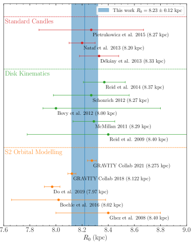
Figure 1: A selection of historical $R_{0}$ measurements using different methods. The vertical blue line and blue colored shaded area show the result and uncertainty from this work.

Pietrukowicz et al. (2015) Dékány et al. (2013) Nataf et al. (2013) Reid et al. (2009a) McMillan (2011) Bovy et al. (2012) Schönrich (2012) Reid et al. (2014) Ghez et al. (2008) Boehle et al. (2016) Gravity Collaboration et al. (2018) Do et al. (2019) Gravity Collaboration et al. (2021)

2 Data

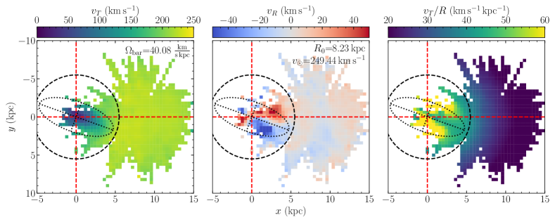
Figure 2: Kinematic maps of the bar and disc of the Milky Way using $R_{0}=8.23\ \mathrm{kpc}$ and $v_{\odot}/R_{0}=30.32\,\mathrm{km\,s}^{-1}\mathrm{kpc}^{-1}$. In each panel, the ellipse with its semi-major and semi-minor axis represented by dotted lines shows the bar with a bar angle of 20^∘. The measured pattern speed from these maps is $40.08\pm 0.65\,\mathrm{km\,s}^{-1}\mathrm{kpc}^{-1}$ (see Section 6.3), which is consistent with Bovy et al. (2019). Comparing to the similar plot in Bovy et al. (2019), which used APOGEE DR16 and Gaia DR2, this plot using APOGEE DR17 and Gaia EDR3 shows a clear, bar-shaped global minimum in tangential velocity and clear blue and red regions separated by the semi-major and semi-minor axis in the radial velocity.

To map the kinematics of the bar region with full six-dimensional phase-space, we use a combination of data from Gaia EDR3 (Gaia Collaboration et al., 2021) and SDSS-IV’s APOGEE’s DR17 (Blanton et al., 2017; Majewski et al., 2017; Abdurro’uf et al., 2022). Briefly, for a sample of stars selected from APOGEE, we obtain sky coordinates and proper motions from Gaia EDR3, line-of-sight velocities from APOGEE, and distances from the astroNN spectro-photometric-distance method from Leung & Bovy (2019b) applied to the APOGEE spectra. In this section, we briefly discuss how we use the different data sets to derive the six-dimensional phase-space data that is the basis of our kinematic maps.

The APO Galactic Evolution Experiment (APOGEE) is a near-infrared ($1.5\ \mu m$ to $1.7\ \mu m$), high resolution ($R\sim 22,500$), high signal-to-noise ratio (typical $\mathrm{SNR}>100$ per pixel for $H<12.2$ with 3 hours of integration) large-scale all-sky spectroscopic survey of Sloan Digital Sky Survey (SDSS) mainly targeting red-giants (Zasowski et al. (2013); Zasowski et al. (2017)). The two 300-fiber cryogenic spectrographs (Wilson et al., 2019) operate at the 2.5-meter Sloan Foundation Telescope (Gunn et al., 2006) at Apache Point Observatory (APO) responsible for the northern celestial hemisphere and 2.5-meter Irénée du Pont Telescope (Bowen & Vaughan, 1973) at Las Campanas Observatory (LCO) responsible for southern the celestial hemisphere. We use data from APOGEE’s latest data release DR17 (Abdurro’uf et al., 2022) where radial velocity, stellar parameters and abundances are derived with the ASPCAP pipeline (Nidever et al., 2015).

We employ the APOGEE data here for two main purposes: (a) to train, test, and evaluate the astroNN spectro-photometric distances using different subsamples of the data and (b) to obtain the line-of-sight velocity of stars in our kinematic sample. For all APOGEE data that we use, we require a line-of-sight velocity scatter $v_{\mathrm{scatter}}<1\ \mathrm{km\,s}^{-1}$, that no STARFLAG flags are set, and that there is a $K_{s}$ band apparent magnitude with corresponding extinction available. We perform additional cuts based on the use case that is detailed below. We solely rely on astroNN-determined stellar parameters and abundances (Leung & Bovy, 2019a) for any cuts based on them below.

We use sky coordinates, parallaxes, and proper motions from Gaia EDR3. Parallaxes are only used to train the astroNN spectro-photometric distances, but they are not directly used in the production of the kinematic maps of the bar. Sky coordinates and proper motions are only used to create the kinematic maps. For the kinematic APOGEE sample, we obtain Gaia EDR3 sky coordinates and proper motions by matching the sky positions with a $2^{\prime\prime}$ matching radius and then use the closest match (this is unambiguous in all cases); the only additional quality cuts on the Gaia EDR3 data for this sample that we apply is that the proper motions cannot be Nan. The proper motion uncertainty is $\approx 0.02\,\mathrm{mas\,yr}^{-1}$ for $G<15$ at which the bulk of our sample lies. For the parallaxes used in the astroNN training, we perform additional quality cuts and corrections.

To obtain distances for our kinematic sample, we have re-trained our neural-network spectro-photometric distance method astroNN by applying the methods from Leung & Bovy (2019b) to the APOGEE DR17 and Gaia EDR3 data (Leung & Bovy 2019b used APOGEE DR14 and Gaia DR2). The input data are improved compared with the original training data in the following ways: (i) the number of APOGEE spectra available has increased by almost $300\%$ to 101,435, (ii) the Gaia EDR3 parallax uncertainty is smaller by about a factor of two, and (iii) the Gaia parallax zero-point is smaller by more than a factor of two as well (Lindegren et al., 2021). By retraining astroNN, we are able to take advantage of these improvements. The resulting improved distances are included as part of the DR17 astroNN VAC (Abdurro’uf et al., 2022).

To construct the training set, we select APOGEE stars with spectral signal-to-noise $\mathrm{SNR}>200$ in addition to the other cuts discussed above. For the training parallaxes from Gaia EDR3, we cut on the Re-normalized Unit Weight Error $\texttt{ruwe}<1.4$, on $\texttt{ip\_frac\_multi\_peak}\leq 2$ and $\texttt{ipd\_gof\_harmonic\_amplitude}<0.1$ (these cuts indicate that a source is non-single, and on parallax uncertainty $\sigma_{\varpi}<0.1\,\mathrm{mas}$. These cuts are adopted from the recommendations in Fabricius et al. (2021) for astrometry from Gaia EDR3. We apply the parallax zero-point correction from Lindegren et al. (2021) and do not fit for it separately (as we did in Leung & Bovy (2019b); we discuss the Gaia zero-point further in Section 3.1. The resulting training set has 101,435 out of all 733,901 APOGEE DR17 stars for training and validation. When training, the parallax is converted to a pseudo-luminosity $L_{\mathrm{pseudo}}=10^{\frac{1}{5}m_{\mathrm{apparent}}}=10^{\frac{1}{5}M_{\mathrm{absolute}}+2}$ from Anderson et al. (2018), where we use the 2MASS $K_{s}$ apparent magnitude and extinction (Skrutskie et al., 2006). This pseudo-luminosity preserves the Gaussianity of the parallax uncertainty when we train the neural network model.

After training, the resulting neural-network spectro-photometric distance accuracy is $\approx 5\ \%$. This is better than Gaia at large distances ($\approx 5\ \mathrm{kpc}$). Because the distance is the most important uncertain ingredient in our data analysis, we validate our distance determinations in more detail in Section 3. When using the astroNN distance for distance validation, we cut on NN $\log g$ uncertainty $<0.15\ \mathrm{dex}$, on Re-normalized Unit Weight Error $\texttt{ruwe}<1.4$ to ensure Gaia astrometric solution quality, within $500\ \mathrm{pc}$ from the mid-plane and Gaia proper motion is not NaN. The rationale for these cuts are discussed in Section 3.

The kinematic sample then consists of all stars in APOGEE DR17 that satisfy $\log g$ uncertainty $<0.15\ \mathrm{dex}$, $0.8<\log g<3.5$ to cut out stars at the edges of parameter space, Re-normalized Unit Weight Error $\texttt{ruwe}<1.4$, and Gaia proper motion is not NaN. This sample has $293,960$ stars in total. To study the kinematics of the bar and disc, we only use stars with vertical distances from the mid-plane less than $500\,\mathrm{pc}$. That sample consists of $138,611$ stars, $16,437$ of which are in the bar region with Galactocentric radii less than 5 kpc. We convert between heliocentric and Galactocentric coordinates using astropy (Astropy Collaboration et al., 2013, 2018). To perform this transformation, we need the position and velocity of the Sun in the Milky Way. Everywhere, we will fix the Sun’s height above the mid-plane to $z_{0}=20.8\,\mathrm{pc}$ (Bennett & Bovy, 2019) and the Sun’s velocity along the radial and vertical direction to $U_{\odot}=11.1\,\mathrm{km\,s}^{-1}$ and $W_{\odot}=7.25\,\mathrm{km\,s}^{-1}$ (Schönrich et al., 2010). The remaining two parameters, $R_{0}$ and the Sun’s velocity $v_{\odot}$ in the rotational direction are varied in our analysis, although we will typically fix $v_{\odot}/R_{0}=30.32\,\mathrm{km\,s}^{-1}\mathrm{kpc}^{-1}$ following Reid et al. (2019).

We use the kinematic sample to make maps of the median Galactocentric rotational velocity $v_{T}$, Galactocentric radial velocity $v_{R}$, and rotational frequency $v_{T}/R$ in the disc and bar region near the mid-plane. For the data, using what we will find to be the best-fit value of $R_{0}$ below, these are shown in Figure 2.

3 Distance accuracy

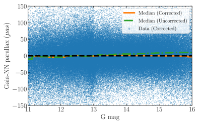
Figure 3: Parallax difference between Gaia EDR3 and the (inverse) astroNN spectro-photometric distance as a function of Gaia $G$ magnitude. The green dotted line shows the median of the parallax difference after adapting the Gaia zero-point correction from Lindegren et al. (2021), while the orange line includes an additional correction of $5(G-13)\mu\mathrm{as}$ for stars with $13<G<16$ (the black dotted line simply shows $y=0$ for reference). The additional linear correction of the orange line is good for at least $13<G<16$ where stars belong to the same window class in the Gaia astrometric calibration pipeline stars with $13\lesssim G\lesssim 16$ belong to WC1).

One of the main factors affecting the accuracy of our $R_{0}$ measurement is the accuracy of the astroNN neural-network distances that we use. Any systematic bias in the astroNN distances will lead to a similar relative bias in our inferred value of $R_{0}$. Systematics in the distances can result from deficiencies in the training set or in the neural-network model itself. Because we train using the Gaia parallaxes, the Gaia parallax zero-point presents a potential issue, especially if the zero-point has complex dependencies on color and ecliptic longitude as shown in Arenou et al. (2018). While in Leung & Bovy (2019b), we also inferred the Gaia zero-point as part of training the neural network, we do not do that here because the zero-point correction presented by Arenou et al. (2018) turns out to be good enough for our purposes (see below). Other deficiencies in the training set can be an issue, such as incomplete or sparse sampling of important parts of parameter space. For example, the luminous giants that we rely on in APOGEE to investigate the bar region are rare locally and, thus, underrepresented in the training set. This sparseness at the edge of the training set can lead to a neural-network model that performs badly at the edge, as predictions tend to regress to the mean located at the less-luminous giants. We discuss these two possible sources of systematics in the following subsections.

3.1 Gaia parallax systematics

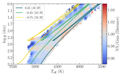
Figure 4: Maximum-likelihood ratio from Equation (1) of the Gaia parallax to the astroNN parallax as a function of $T_{\mathrm{eff}}$ and $\log g$ within $0.5\,\mathrm{kpc}$ of the Galactic plane and including only stars with $G<16$ for reasons discussed in Figure 3 and Section 3.1. Each bin has a width of $20\,\mathrm{K}$ in $T_{\mathrm{eff}}$ and of $0.03\,\mathrm{dex}$ in $\log g$; we only display bins with ten or more stars. PARSEC isochrones (Bressan et al., 2012) for an age of $5\ \mathrm{Gyr}$ are over-plotted to give a sense of where $-0.75$ $[\mathrm{M/H}]$ to $0.25$ $[\mathrm{M/H}]$ tracks are located. The Gaia parallaxes on average agree with the astroNN parallaxes to about a percent in the well-populated parts of stellar-parameter space and at worst disagree by a few percent.

The Gaia parallaxes are known to suffer from a zero-point issue at least partially caused by the variation of the basic angle between the two fields of view that Gaia employs (Butkevich et al., 2017) and also because of deficiencies in the data processing pipeline. The zero-point correction is not only important in the training of the astroNN distances, but also in the validation of our distances that we present in this section. Normally, neural networks transfer any systematics present in the training data to the network and, thus, to any outputs derived from it. But we are not directly training on the Gaia parallaxes when training the astroNN model, instead the model predicts a pseudo-luminosity that needs to be combined with a star’s apparent magnitude to obtain the distance. Because the Gaia zero-point cannot be predicted directly from the APOGEE spectra, the astroNN will transfer the average effect of the parallax zero-point as a result. However, this could still lead to systematic biases.

Unlike in Leung & Bovy (2019b), we fix the Gaia parallax zero-point during the training rather than fitting for it and we fix it to the model from Lindegren et al. (2021). Numerous other works have independently validated the accuracy of the Lindegren et al. (2021) correction. For example, Zinn (2021) validated the correction using stars with astrometric distances in the APOGEE-Kepler field and they report that the Lindegren et al. (2021) zero-point correction for the five-parameters astrometric solution, which is the relevant case for almost all APOGEE stars, is good within $2\ \mu\mathrm{as}$ at $G<13$. However, they do not cover $G>13$ due to a lack of stars at these magnitudes in their sample, which is not ideal because we do depend on these stars and the Gaia instrument and pipeline processes data at these magnitudes differently due to the use of astrometric window classes. Stars with $G>13$ are particularly of interest due to the high level of extinction towards the bar. Huang et al. (2021) validated the Gaia zero-point correction using LAMOST primary red-clump stars and they report that the zero-point over-corrects the parallaxes for stars with $G>14$ in the five-parameters astrometric solution.

To investigate the appropriateness of the Lindegren et al. (2021) correction, Figure 3 shows the parallax difference between Gaia and our astroNN distances as a function of Gaia $G$ magnitude. The parallax zero-point is known to be a non-trivial function of magnitude, color, sky position, etc. Most of the zero-point’s dependencies cannot be inferred from spectra alone, thus, they do not affect the resulting spectro-photometric distances (discussed extensively in Leung & Bovy 2019b). Without the presence of any parallax bias there should be no median difference between Gaia and astroNN parallaxes, but any parallax bias from Gaia will show up as a trend as a function of zero-point dependencies. Thus, by looking for trends in the difference between Gaia and astroNN parallaxes, we can test for the presence of remaining zero-point systematics in Gaia. The green line is the median as a function of $G$ and we observe an over-correction at faint end similar to that found by Huang et al. (2021). The over-correction is clearly seen to start at $G>13$, which is unsurprising as it is a break-point in Gaia’s astrometric analysis. In Figure 3, the orange dotted line (median) and the blue scattered points (individual stars) both display the difference after an additional correction of $5(G-13)\,\mu\mathrm{as}$ for stars with $13<G<16$. It is clear that this succeeds in flattening the green curve. Thus, we find that the Lindegren et al. (2021) correction should be slightly altered at $13<G<16$. While ideally we would apply this new correction before training the astroNN distance network, stars with $13<G<16$ are sufficiently rare in the training set, because of our signal-to-noise ratio cut, that the trained network is hardly affected by this change. We have explored retraining the model after applying the additional correction, but find no significant difference in the predicted distances. Therefore, we continue to use the original distances in this paper (these are the ones in the official astroNN VAC and this choice therefore makes it easier to reproduce our results). However, we do apply the additional correction in the next section when validating our astroNN distances, because stars with $13<G<16$ are common at large distances and while the astroNN distance does not depend on the additional correction, the Gaia parallaxes that we use to validate our distances do strongly depend on them.

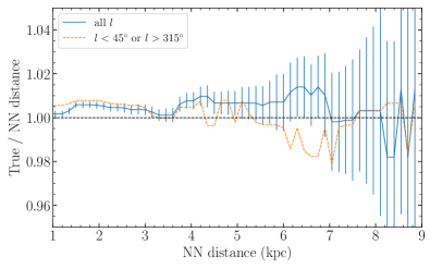
Figure 5: Ratio of the true distance to the astroNN spectro-photometric distance as a function of astroNN distance ranging from $1\,\mathrm{kpc}$ to $9\,\mathrm{kpc}$ within $0.5\,\mathrm{kpc}$ of the Galactic mid-plane. Only stars with $G<16$ are used and an additional zero-point correction of $5(G-13)\mu\mathrm{as}$ for stars with $13<G<16$ is applied ton the Gaia parallaxes for the reasons discussed in Figure 3 and Section 3.1. The true distance is the distance inferred from a robust maximum-likelihood stacking of the Gaia parallaxes in $0.15\,\mathrm{kpc}$ wide bins in astroNN distance (Equation 2). The error bars are statistical uncertainty determined by bootstrap re-sampling; they are correlated because neighbouring bins overlap. The blue line employs all of the stars, while the orange line only uses stars within the direction to the bar. The ratio is almost always within $1\%$ for both lines showing that the astroNN distance accuracy is $\lesssim 1\%$.

3.2 astroNN distance systematics

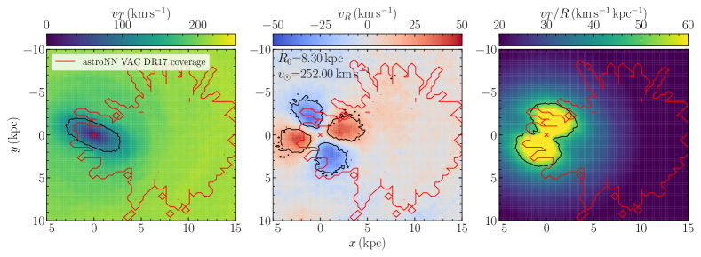
Figure 6: Kinematic maps of the bar and disc for the simulation from Kawata et al. (2017). The bar pattern speed ground truth is $24.5\,\mathrm{km\,s}^{-1}\mathrm{kpc}^{-1}$ at a $25^{\circ}$ bar angle. Each bin has a width of $0.2\,\mathrm{kpc}$. The red contours represent the area covered by the APOGEE data in the Milky Way.

The neural-network model used to train and evaluate the astroNN distances can introduce distance systematics, for example, if important parts of parameter space are sparsely covered by training data or at the edges of parameter space, where predictions will tend to regress to the mean. Because we depend on luminous giants in APOGEE to reach the Galactic bar region, which are rare in the training sample with high signal-to-noise ratio spectra and located near the edge of parameter space, both of these effects are highly relevant.

We investigate the presence of any systematic biases in the astroNN distances in this sub-section. Figure 4 displays the ratio between the Gaia parallax with the additional $G$-mag dependent correction shown in Figure 3 and the inverse astroNN distance (i.e., the astroNN parallax). We robustly determine the ratio in bins of $T_{\mathrm{eff}}$ and $\log g$ by assuming that stars in the same $T_{\mathrm{eff}}$$\log g$ bin have similar luminosities. The space of $T_{\mathrm{eff}}$ and $\log g$ is a logical choice of parameter space, because the neural-network model predicts spectro-photometric distances from spectra, and therefore, features like $T_{\mathrm{eff}}$, $\log g$, and metallicity dominate the features used by the network. The feature $\log g$ is a particularly important for predicting the luminosity. In the absence of any distance bias, we expect that the shown parallax ratio is one in each bin. Our robust estimate of the ratio in each bin is obtained using a maximum-likelihood-like method by minimizing

$$\min_{\Delta}\qquad\sum_{i}{\left|\frac{\varpi_{\mathrm{i,gaia}}}{\varpi_{\mathrm{i,NN}}}-\Delta\right|\frac{1}{\sigma_{\varpi,i}}}$$ (1)

for $\Delta$, the inferred parallax ratio. Most stars are within only a few percent in Figure 4 except in some parts of the metal-poor end of the diagram that is sparsely covered in the training set. The median of $|1-\Delta|\approx 1\%$ for the bins displayed in Figure 4.

To test in more detail for the presence of distance biases in the Galactic bar region, we also examine how distance biases vary as a function of distance in Figure 5. In this figure, we present a similar check as first performed by Bovy et al. (2019): we assume that if astroNN states that two stars are at the same distance, they truly are so, even if astroNN might return a biased distance. Thus, we can create large samples of stars at a given distance. For these, we can statistically stack the Gaia parallaxes (corrected for zero-point offsets) and determine the true, geometric distance that provides a good check for distance biases. Specifically, for stars in a bin of astroNN distance, we infer the Gaia distance by minimizing

$$\min_{D}\qquad\sum_{i}\frac{|\varpi_{i}-1/D|}{\sigma_{\varpi,i}}$$ (2)

where $D$ is the true distance that minimize the equation for each distance bin. Figure 5 displays the resulting ratio between the true and the astroNN distance as a function of astroNN distance for all stars within $0.5\,\mathrm{kpc}$ from the mid-plane as well as for those stars towards the bar region. The ratio is almost always within $1\%$ in both cases.

The tests shown in Figure 4 and Figure 5 demonstrate that our astroNN distances have systematic biases $\lesssim 1\%$, or about $80\,\mathrm{pc}$ at the distance of the Galactic center.

4 Methodology

Stars in the Milky Way disc and bar rotate around the center with a mean tangential velocity $\langle v_{T}\rangle$. The $m=2$ symmetry of the bar requires that $\langle v_{T}\rangle$ reaches an extremum at the location of the barycenter of the Milky Way. Simulations such as the ones that we discuss below demonstrate that this extremum is a minimum at $\langle v_{T}\rangle\approx 0$ for galaxies with bars similar to that of the Milky Way. It is this minimum in $\langle v_{T}\rangle$ that we use to determine $R_{0}$.

Figure 6 shows similar kinematic maps of the mean $v_{T}$, $v_{R}$, and $v_{T}/R$ for the simulation of a barred Milky-Way-like galaxy from Kawata et al. (2017). This simulation does not include a supermassive black hole at the center or gas, but a comparison with the kinematic maps of the data in Figure 2 demonstrates that they are similar and the simulation therefore matches the dynamics in the bar region well despite its limitations. We have oriented the bar at an angle of $25^{\circ}$ to approximately match the bar angle in the Milky Way. Figure 6 displays the data correctly, that is, without distorting them by using an incorrect value of $R_{0}$. We also overlay the approximate footprint of the data kinematic maps (which is driven by APOGEE’s selection function). We see multiple signatures pinpointing the location of the galactic center. The mean rotational velocity $v_{T}$ shows a well-defined minimum at the center, while the radial velocity $v_{R}$ displays a saddle point, and the rotational frequency $v_{T}/R$ a maximum. The radial velocity map also displays a distinct clover-leaf pattern of high and low radial velocities within the bar region. This clover-leaf pattern also locates the galactic center. However, it does not do so as clearly as the minimum in $v_{T}$.

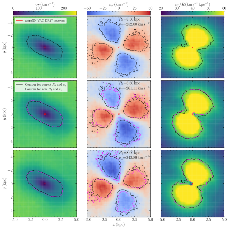
Figure 7: Kinematic maps like in Figure 6, but zooming in on the central region and including the effects of assuming the wrong galactic parameters. The different rows use different sets of $R_{0}$ and $v_{\odot}$ while keeping $v_{\odot}/R_{0}$ fixed at $\approx 30.32\,\mathrm{km\,s}^{-1}\mathrm{kpc}^{-1}$. The top row uses the true $R_{0}$ and $v_{\odot}$ ($R_{0}=8.3\,\mathrm{kpc}$ and $v_{\odot}252.00\,\mathrm{km\,s}^{-1}$). The second row uses an $R_{0}$ offset by $0.3\,\mathrm{kpc}$ and $v_{\odot}=261.11\,\mathrm{km\,s}^{-1}$, while the third row uses an $R_{0}$ offset by $-0.3\,\mathrm{kpc}$ and $v_{\odot}=242.89\,\mathrm{km\,s}^{-1}$. The red cross in each panel always highlights the location of the center at $(0,0)$. The black contours in all three rows shows the contours of $120\,\mathrm{km\,s}^{-1}$ for $v_{T}$, $20\,\mathrm{km\,s}^{-1}$ for $v_{R}$, and $50\,\mathrm{km\,s}^{-1}\mathrm{kpc}^{-1}$ for $v_{T}/R$ using the correct set of $R_{0}$ and $v_{\odot}$, while in the second and third row, the purple contours represent the same levels for the incorrect set of $R_{0}$ and $v_{\odot}$.

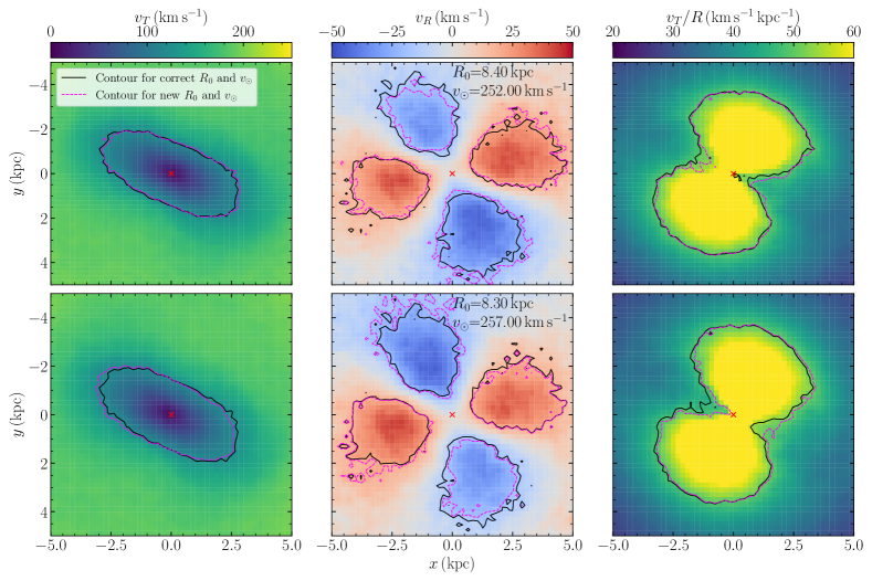
Figure 8: Like the middle and bottom row of Figure 7, but changing $R_{0}$ and $v_{\odot}$ without keeping $v_{\odot}/R_{0}$ constant. Comparing to Figure 6, a small offset in either $R_{0}$ or $v_{\odot}$ produces more significant shifts in the kinematic maps than offsets in $R_{0}$ and $v_{\odot}$ that keep $v_{\odot}/R_{0}$ fixed.

Figure 7 contains a zoomed-in version of Figure 6 as the top row and the middle and bottom row shows what happens when we create the kinematic maps of the simulation using wrong values of $R_{0}$ and the Sun’s rotational velocity $v_{\odot}$—this $v_{\odot}$ is the second most important parameter that has to be assumed to make the kinematic maps in the Galactocentric frame—but keeping the value of $v_{\odot}/R_{0}$ constant. That is, we convert the simulation’s phase-space data to the heliocentric coordinates of a mock observer located at $R=8.3\,\mathrm{kpc}$, $\phi=z=0$, $v_{\odot}=252\,\mathrm{km\,s}^{-1}$, and $U_{\odot}=W_{\odot}=0$. We then convert these coordinates back to Galactocentric coordinates assuming a wrong value of $R_{0}$ and $v_{\odot}$.

The left panels clearly demonstrate that the location of the minimum shifts away from $(0,0)$, while the middle panels show that the saddle point in $v_{R}$ remains approximately at $(0,0)$. The change in the $v_{R}$ pattern is therefore more subtle and, thus, more difficult to detect: the leafs of the clover become asymmetric (compare the purple contours of simulations with the wrong parameters to the symmetric contours of the simulation with the correct parameters), but this is difficult to detect without full coverage of the bar region. While the maximum in $v_{T}/R$ does shift away from $(0,0)$, we do not use it, because (i) it does not contain different information from $v_{T}$ and (ii) the maximum’s value is less universal.

Figure 8 shows another two sets of wrong values for $R_{0}$ or $v_{\odot}$, but this time not keeping the ratio $v_{\odot}/R_{0}$ constant. Comparing to Figure 6, we see that the changes to the contours in $v_{R}$ and $v_{T}/R$ are similar, even though the changes to $R_{0}$ and $v_{\odot}$ are much smaller than those in Figure 6. Thus, when $v_{\odot}/R_{0}$ is well constrained, constraining $R_{0}$ using $v_{R}$ or $v_{T}/R$ is more difficult, while the minimum in $v_{T}$ remains sensitive to $R_{0}$ shifts.

To investigate the universality of the minimum in $v_{T}$ that we observe in Figure 6, we also consider kinematic maps created from the simulation suite presented by Bennett et al. (2022), which includes unperturbed Milky-Way-like galaxies as well as galaxies perturbed by the Sgr dwarf galaxy. Figure 9 shows an example kinematic $v_{T}$ map from one of their simulations, which is perturbed by the infall of the massive Sgr dwarf. It is clear from this figure that this simulated bar does not have as clear of a minimum as the simulation in Figure 6 and there is some structure along the minor axis that is not present in the simulations from Kawata et al. (2017). Nevertheless, running the fitting routine described below on the data in Figure 9 returns the correct value of $R_{0}$ albeit with larger uncertainties. The other simulations in the suite from Bennett et al. (2022) give similar results. Because the observed kinematic maps resemble those from Figure 6 more than they do that in Figure 9 (which is also seen by Eilers et al. 2021 using the spectro-photometric distances from Hogg et al. 2019), they provide a more realistic test of our method.

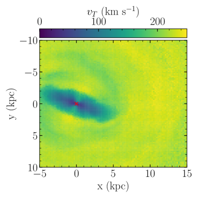
Figure 9: Kinematic $v_{T}$ map from a Milky-Way-like simulation Milky-Way disc presented in Bennett et al. (2022). The simulated disc is perturbed by the infall of a massive Sgr-like dwarf. The red cross show the location of the galactic center at $(0,0)$. The figure shows that $v_{T}$ is approximately constant near the center without showing as clear of a minimum as for the simulation presented in Figure 6 or as in the real data from Figure 2. Nevertheless, applying our fitting routine returns the correct value of $R_{0}$ for this simulation, albeit with larger uncertainties than for the simulation in Figure 6.

The current footprint of the data (shown by the red contours in Figure 6) clearly limits our use of the data: as discussed above, detecting the subtle changes in the clover-leaf pattern in $v_{R}$ is difficult with this footprint, and even in $v_{T}$ we do not have a wide range of Galactocentric azimuths. To keep things simple, therefore, we only use $v_{T}$ along the $y=0$ axis, that is, we use a one-dimensional slice of the kinematic maps along the center-Sun line. The main advantage of this is that it makes the creation of an objective function to minimize simple.

To find the minimum in $v_{T}$, we calculate the smoothed running median using sliding window of $v_{T}$ along the x-axis (with $|y|<0.5\,\mathrm{kpc}$) for the stars in our kinematic sample within $500\ \mathrm{pc}$ from mid-plane. Then we find the value of $R_{0}$ that minimizes the following objective function:

$$\min_{R_{0}}\qquad f\left(R_{0},v_{\odot}[R_{0}]\right)=\sqrt{\left(\frac{x_{i}}{2\ \mathrm{kpc}}\right)^{2}+\left(\frac{v_{T,i}}{50\ \mathrm{km\,s}^{-1}}\right)^{2}}$$ (3)

where the scaling parameters $2\ \mathrm{kpc}$ and $50\ \mathrm{km\,s}^{-1}$ are chosen to approximately scale both $R$ and $v_{T}$ onto the same scale. The rotational velocity $v_{T,i}$ is the value of the running median at positions $x_{i}$ indexed by $i$. We always use $R_{0}$ and $v_{\odot}/R_{0}$ as the independent parameters, so $v_{\odot}(R_{0})=R_{0}\times v_{\odot}/R_{0}$ when we vary the assumed value of $v_{\odot}/R_{0}$.

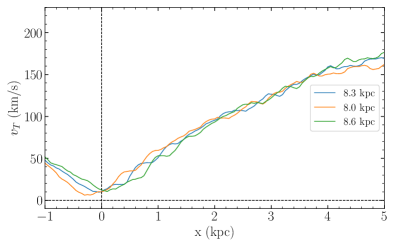
Figure 10: Median tangential velocity $v_{T}$ for stars in the simulation from Kawata et al. (2017) that are $\pm 0.5\,\mathrm{kpc}$ from the $x$-axis smoothed by a Gaussian kernel. The median velocity $v_{T}$ is calculated for $R_{0}=8.0\,\mathrm{kpc}$, $8.3\,\mathrm{kpc}$ (the correct value), and $8.6\,\mathrm{kpc}$. For the correct $R_{0}$, a minimum in $v_{T}$ is observed near the origin. For incorrect values of $R_{0}$, the minimum occurs away from $x=0$ and at larger values of $v_{T}$. This figure is similar to Figure 12 for the real data.

We apply this fitting routine to the simulations from Kawata et al. (2017) shown in Figure 6, using different true values of $R_{0}$ for the heliocentric observer in the simulation. The value of the median $v_{T}$ as a function of $x$ for three different true values of $R_{0}$ is shown in Figure 10, where the correct minimum should occur at $x=0$. This figure demonstrates that we successfully recover $R_{0}$ to an accuracy of $\approx 0.05\,\mathrm{kpc}$.

5 Result

We determine $R_{0}$ using the kinematic sample by optimizing the objective function in Equation (3) and we obtain its random uncertainty by bootstrapping the kinematic sample (that is, we create new kinematic samples of the same size by re-sampling with replacement from the original one). To account for the uncertainty in the angular Galactocentric velocity $v_{\odot}/R_{0}$ of the Sun, we use the measurement of $v_{\odot}/R_{0}=30.32\pm 0.27\ \mathrm{km\,s}^{-1}\mathrm{kpc}^{-1}$ from Reid et al. (2019) in the following way. To determine our best-fit value of $R_{0}$, we fix $v_{\odot}/R_{0}=30.32\,\mathrm{km\,s}^{-1}\mathrm{kpc}^{-1}$, but when determining the uncertainty in $R_{0}$, we sample from a Gaussian distribution with a mean of $v_{\odot}/R_{0}=30.32\,\mathrm{km\,s}^{-1}\mathrm{kpc}^{-1}$ and a standard deviation that is eight times the uncertainty from Reid et al. (2019): $\sigma_{v_{\odot}/R_{0}}=2.16\,\mathrm{km\,s}^{-1}\mathrm{kpc}^{-1}$. We use eight times the stated uncertainty as the standard deviation to be very conservative in our assumption about $v_{\odot}/R_{0}$. Because the measurement from Reid et al. (2019) is based on the kinematics of masing high-mass star-forming regions in the disk, it is independent from Sgr A^∗ and our adoption of $v_{\odot}/R_{0}$ from Reid et al. (2019) therefore does not introduce any dependence on Sgr A^∗ being at the center of the Milky Way.

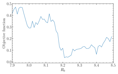
Figure 11: Objective function from Equation 3 for a range of possible values of spanning the range of historical measurements. The objective function displays a minimum at $R_{0}=8.23\pm 0.12\,\mathrm{kpc}$. Values of $R_{0}\lesssim 8.15\,\mathrm{kpc}$ are especially disfavored.

The resulting measurement is $R_{0}=8.23\pm 0.12\,\mathrm{kpc}$. Figure 11 shows the objective function for $v_{\odot}/R_{0}=30.32\,\mathrm{km\,s}^{-1}\mathrm{kpc}^{-1}$. It displays a clear minimum at $R_{0}\approx 8.2\,\mathrm{kpc}$. Values of $R_{0}\lesssim 8.15\,\mathrm{kpc}$ in particular lead to large values of the objective function and are, thus, disfavored. This clearly rules out the lower end of historical $R_{0}$ measurements shown in Figure 1.

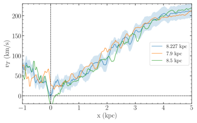
Figure 12: Median tangential velocity $v_{T}$ for stars in the kinematic sample that are $\pm 0.5\,\mathrm{kpc}$ from the $x$-axis smoothed by a Gaussian kernel. The median velocity $v_{T}$ is calculated for $R_{0}=7.90\,\mathrm{kpc}$, $8.50\,\mathrm{kpc}$, and $8.23\,\mathrm{kpc}$—our optimal value of $R_{0}$. All curves use $v_{\odot}/R_{0}=30.32\,\mathrm{km\,s}^{-1}\mathrm{kpc}^{-1}$ from Reid et al. (2019). The blue band shows the effect of varying $v_{\odot}/R_{0}$ within $8\sigma$ of the Reid et al. (2019) measurement, which translates to about a $9\,\mathrm{km\,s}^{-1}$ variation in solar tangential velocity. For the optimal $R_{0}$, a minimum in $v_{T}$ at $\approx 0\,\mathrm{km\,s}^{-1}$ near the origin is observed $\approx 0.05\ \mathrm{kpc}$ away from $x=0$, well within the accuracy of our astroNN spectro-photometric distances. For non-optimal values of $R_{0}$, the minimum occurs away from $x=0$ and at larger values of $v_{T}$.

Figure 12 displays $v_{T}$ as a function of $x$ for a few values of $R_{0}$. We see that for assumed values of $R_{0}$ away from the best-fit value, the minimum of the curve both shifts away from $x=0$ and the minimum has a higher $v_{T}$ value. Both of these indicate that these values of $R_{0}$ are disfavored. We also shows the effect of varying $v_{\odot}/R_{0}$ within its assumed uncertainty (eight times the nominal uncertainty from Reid et al. 2019) as a band around the curve for the best-fit value of $R_{0}$. It is clear that our solution is not very sensitive to the choice of $v_{\odot}/R_{0}$.

The kinematic maps of the disc and bar region using our optimal value of $R_{0}$ and $v_{\odot}/R_{0}=30.32\,\mathrm{km\,s}^{-1}\mathrm{kpc}^{-1}$ from Reid et al. (2019) is shown in Figure 2. In this figure, the left panel showing $v_{T}$ displays a minimum that is clearly shaped like a bar and the middle $v_{R}$ panel shows clear blue and red regions separated by the semi-major and semi-minor axes of the bar. Comparing these maps to those determined from the Milky-Way-like simulation in Figure 6, we see that they are remarkably similar.

6 Discussion

We have presented a new measurement of the distance $R_{0}$ to the Galactic center using the kinematics of stars in the Galactic bar. In this section, we compare our measurement to other recent measurements of $R_{0}$, we consider the implications for Sgr A^∗, and we derive an updated measurement of the bar’s pattern speed using the method of Bovy et al. (2019) applied to the kinematic maps of Figure 2.

6.1 Comparison to other recent measurements of $R_{0}$

We compare our determination of $R_{0}=8.23\pm 0.12\,\mathrm{kpc}$ to a selection of other recent measurements in Figure 1. Visually, it is immediately clear that our measurement has a smaller uncertainty than essentially all but the S2-based measurements (Gravity Collaboration et al., 2018; Do et al., 2019; Gravity Collaboration et al., 2021) (the Nataf et al. 2013 measurement being a notable exception that agrees well with ours). Bland-Hawthorn & Gerhard (2016) summarized measurements up to $\approx 2016$ (thus excluding the recent, high-precision S2-based measurements) and derived an overall best estimate of $R_{0}=8.2\pm 0.1\,\mathrm{kpc}$. This is in remarkably good agreement with our own measurement here both in value and uncertainty, but the value derived by Bland-Hawthorn & Gerhard (2016) is a consensus value based on all pre-2016 measurements, while ours is a measurement based on a single simple and robust signature of the Galactic center.

The most recent S2-based measurements using the GRAVITY instrument and using Keck have achieved high precision by taking advantage of S2’s 2018 pericentric passage around Sgr A^∗. The resulting precision is about a factor of 2 to 4 better than our measurement. However, all S2-based (or, more generally, Sgr A^∗-based) measurements have to assume that Sgr A^∗ is located at the center of the Milky Way. This does not have to be the case for a variety of reasons that are discussed in more detail in the next section: Sgr A^∗ might not be at rest at the Galactic center even if it is orbiting the true center, or the nuclear star cluster (NSC) that contains Sgr A^∗ might be sloshing around within the bar/disc system. In both cases, the offset between Sgr A^∗ and the true barycenter can be larger than the current measurement uncertainties. Our measurement, on the other hand, is unambiguously of the barycenter of the bar/disc system, which are coupled because the bar is an integral dynamical part of the disc, and this is likely the actual barycenter. More prosaically, the S2-based methods are still somewhat plagued by instrumental effects like aberrations and by the difficulty of tying the small field-of-view reference frame to a global one. The difference between the Do et al. (2019) and Gravity Collaboration et al. (2021) measurements (and the significant differences between different iterations of the GRAVITY measurements based on similar data) demonstrate that these remain real issues and that the true uncertainty of the S2-based methods is likely larger than their reported uncertainty. Indeed, simply splitting the difference between Do et al. 2019 and Gravity Collaboration et al. 2021 as an estimate of their true uncertainty gives $R_{0}\approx 8.15\pm 0.15\,\mathrm{kpc}$, consistent with our own measurement with similar uncertainty.

6.2 Implications for the position and motion of Sgr A^∗

As discussed above, recent measurements of $R_{0}$ based on the orbit of the star S2 around Sgr A^∗ have achieved very high precision, but these measurements have to assume that Sgr A^∗ is located at the barycenter of the Milky Way. This may not be the case. A supermassive black hole at the center of a dense NSC like the Milky Way’s will perform Brownian motion resulting from the random combined kicks from passing stars (Chatterjee et al., 2002; Merritt et al., 2007). The agreement between the value of $v_{\odot}/R_{0}=30.32\pm 0.27\,\mathrm{km\,s}^{-1}\mathrm{kpc}^{-1}$ obtained from the kinematics of masers (Reid et al., 2019) and the value $v_{\odot}/R_{0}=30.39\pm 0.04\,\mathrm{km\,s}^{-1}\mathrm{kpc}^{-1}$ obtained from the proper motion of an assumed-at-rest Sgr A^∗ (Reid & Brunthaler, 2020) demonstrates that the velocity of this Brownian motion is $\lesssim 0.27\,\mathrm{km\,s}^{-1}\mathrm{kpc}^{-1}\times R_{0}\approx 2\,\mathrm{km\,s}^{-1}$. For the $\gtrsim 10^{6}\,M_{\odot}\,\mathrm{pc}^{-3}$ density of the NSC, this would lead to a spatial offset $\ll 1\,\mathrm{pc}$. Brownian motion of Sgr A^∗ within the NSC on its own is therefore not a significant issue in determining $R_{0}$ using Sgr A^∗.

Even if Sgr A^∗ is at the center of the NSC, it is possible that the entire NSC is moving with respect to the barycenter of the entire Milky Way. The NSC may have formed through the accretion of a dense stellar system and in this case, the NSC sinks to the Galactic center through dynamical friction. However, if the stellar density is cored near the center—as direct measurements of the stellar density hint it might be within the central few hundred pc (Wegg & Gerhard, 2013)—the inspiraling NSC may stall near the core radius (Petts et al., 2016). The NSC and Sgr A^∗ may therefore find itself $\approx 100\,\mathrm{pc}$ away from the barycenter of the bar/disc. Observational determinations of the locations of supermassive black holes relative to the centers of their host galaxies indeed show that $\approx 100\,\mathrm{pc}$ offsets are common (see Fig. 1 and references in Bartlett et al. 2021). The agreement between non-Sgr-A^∗-based and Sgr-A^∗-based measurements of $v_{\odot}/R_{0}$ again limit the velocity of the motion of the NSC to be $\lesssim 2\,\mathrm{km\,s}^{-1}$, implying that we should be seeing the NSC near a turning point if its orbit extends out to $\approx 100\,\mathrm{pc}$. While this is unlikely, it is within the realm of possibility. The agreement between our $R_{0}$ measurement and the Sgr-A^∗-based ones shows that the offset between the NSC and the barycenter is $\lesssim 100\,\mathrm{pc}$, consistent with the previous considerations without providing a stringent constraint on them.

6.3 Pattern Speed

Because the Galactic bar dominates the mass distribution in the central regions of our Galaxy, determining its properties is essential to understanding the co-evolution of the bar and the other Galactic components and for studying the dynamics of stars in the bar, disc, and halo (e.g., Pearson et al. 2017; Hunt & Bovy 2018; Antoja et al. 2018; Banik & Bovy 2019; Fragkoudi et al. 2019). One of the most important properties that has been historically challenging to measure is the bar’s pattern speed $\Omega_{\mathrm{bar}}$. Because the bar’s pattern speed sets the locations of resonances in the disc and halo, its exact value is important for, e.g., the interpretation of the velocity structure near the Sun in terms of bar and spiral resonances (e.g., Hunt et al. 2019; Trick et al. 2021. Measurements over the last decade have found a wide range of pattern speeds, with disc-kinematic measurements finding $\Omega_{\mathrm{bar}}\approx 50\,\mathrm{km\,s}^{-1}\mathrm{kpc}^{-1}$ by assuming that the solar-neighbourhood Hercules stream is caused by the 2:1 outer Lindblad resonance (e.g., Antoja et al. 2014), gas kinematics in the bar finding $\Omega_{\mathrm{bar}}\approx 33\,\mathrm{km\,s}^{-1}\mathrm{kpc}^{-1}$ (Li et al., 2016), and stellar kinematics preferring values at $\Omega_{\mathrm{bar}}\approx 40\,\mathrm{km\,s}^{-1}\mathrm{kpc}^{-1}$ Portail et al. (2017); Sanders et al. (2019); Bovy et al. (2019).

Bovy et al. (2019) presented a purely-kinematic measurement of $\Omega_{\mathrm{bar}}$ based on the application of the continuity equation (similar to the famous Tremaine & Weinberg 1984 method) to the kinematic maps of $v_{T}$ and $v_{R}$ in the bar region. They found $\Omega_{\mathrm{bar}}=41\pm 3\,\mathrm{km\,s}^{-1}\mathrm{kpc}^{-1}$ using similar data as we use here, but based on the earlier APOGEE DR16, Gaia DR2, and astroNN VAC DR16 data. For this measurement, they assumed a fiducial value of $R_{0}=8.125$ based on Gravity Collaboration et al. (2018) and $v_{\odot}=242\,\mathrm{km\,s}^{-1}$. Repeating their measurement with the kinematic maps derived here that are shown in Figure 2 and using our best-fit value of $R_{0}=8.23\,\mathrm{kpc}$ combined with $v_{\odot}=249.44\,\mathrm{km\,s}^{-1}$ (from combining $R_{0}$ with $v_{\odot}/R_{0}=30.32\,\mathrm{km\,s}^{-1}\mathrm{kpc}^{-1}$), we find $\Omega_{\mathrm{bar}}=40.08\pm 0.65\,\mathrm{km\,s}^{-1}\mathrm{kpc}^{-1}$ where the uncertainty is purely statistical. This measurement is consistent with the measurement from Bovy et al. (2019), but slightly lower and with smaller statistical uncertainties (the statistical uncertainty in Bovy et al. 2019 was $1.5\,\mathrm{km\,s}^{-1}\mathrm{kpc}^{-1}$).

Systematics in the measurement of $\Omega_{\mathrm{bar}}$ come in two flavours: model uncertainty about how well the method and its assumption work for a galaxy like the Milky Way and uncertainty in the adopted Galactic parameters $R_{0}$ and $v_{\odot}$. By applying the method to simulated galaxies that are realistic representations of the Milky Way’s dynamics (including the simulation from Kawata et al. 2017), Bovy et al. (2019) showed the model uncertainty to be $\approx 1.5\,\mathrm{km\,s}^{-1}$ and this uncertainty remains. However, our improved measurement of $R_{0}$ leads to a decreased systematic uncertainty from the Galactic parameters. Table 1 gives the measured $\Omega_{\mathrm{bar}}$ for different sets of $R_{0}$ and $v_{\odot}$ to investigate this source of systematic uncertainty. The top section varies $R_{0}$ in the range $8.0$ to $8.4\,\mathrm{kpc}$ while keeping $v_{\odot}/R_{0}$ fixed to its fiducial value. In this case, $\Omega_{\mathrm{bar}}$ barely changes by $\approx 0.2\,\mathrm{km\,s}^{-1}\mathrm{kpc}^{-1}$. The middle section shows what happens if we change $R_{0}$ or $v_{\odot}$ independently from their fiducial values by a large amount (compared to the uncertainties). In this case, $\Omega_{\mathrm{bar}}$ changes significantly. Thus, the pattern speed is mainly affected by the solar tangential velocity, with only a minor effect from the uncertainty in $R_{0}$. The bottom section then more rigorously considers the effect of changing $v_{\odot}/R_{0}$ within its uncertainties from Reid et al. (2019): when varying $v_{\odot}/R_{0}$ by $1\sigma$, $\Omega_{\mathrm{bar}}$ changes by $0.7\,\mathrm{km\,s}^{-1}\mathrm{kpc}^{-1}$ (we also show the $8\sigma$ range considered previously to show the effect of large changes in $v_{\odot}/R_{0}$). Thus, the systematic uncertainty from the Galactic parameters is $\approx 0.7\,\mathrm{km\,s}^{-1}\mathrm{kpc}^{-1}$, about the same as the random uncertainty in the measurement. Note that we do not use the measurement of $v_{\odot}/R_{0}$ from Reid & Brunthaler (2020) that is derived from the proper motion of Sgr A^∗ even though it has smaller uncertainties, because of the possibility of Brownian motion of Sgr A^∗ (see the discussion in Section 6.2 above).

Thus, our measurement of the pattern speed is

$$\Omega_{\mathrm{bar}} =40.08\pm 0.65\,(\mathrm{stat.})\,\pm 0.70\,(v_{\odot}/R_{0}\,\mathrm{unc.})$$ (4)

$$\ \ \quad\qquad\pm 1.5\,(\mathrm{model\ unc.})\,\mathrm{km\,s}^{-1}\mathrm{kpc}^{-1}\,,$$

$$=40.08\pm 1.78\,\mathrm{km\,s}^{-1}\mathrm{kpc}^{-1}\,,$$ (5)

where in the last line we have combined all the different sources of uncertainty into a single number.

$R_{0}\ (\mathrm{kpc})$	$v_{\odot}\ (\mathrm{km\,s}^{-1})$	$\frac{v_{\odot}}{R_{0}}\ (\mathrm{km\,s}^{-1}\mathrm{kpc}^{-1})$	$\Omega_{\mathrm{bar}}\ (\mathrm{km\,s}^{-1}\mathrm{kpc}^{-1})$
8.23	249.44	30.32	$40.08\pm 0.65$
8.00	242.56	30.32	$39.90\pm 0.75$
8.40	254.69	30.32	$39.95\pm 0.61$
8.00	249.44	31.18	$42.00\pm 0.71$
8.23	240.00	29.17	$37.25\pm 0.64$
8.23	247.22	$30.32-0.27$	$39.36\pm 0.63$
8.23	251.66	$30.32+0.27$	$40.78\pm 0.65$
8.23	231.67	$30.32-2.16$	$34.85\pm 0.69$
8.23	267.21	$30.32+2.16$	$44.12\pm 0.69$

Table 1: Pattern speed $\Omega_{\mathrm{bar}}$ measurement using different sets of $R_{0}$ and $v_{\odot}$. The first row uses the best-fit $R_{0}$ from this paper combined with the $v_{\odot}/R_{0}$ measurement from Reid et al. (2019). The top section shows the result of changing $R_{0}$ while keeping $v_{\odot}/R_{0}$ fixed. The middle section varies $R_{0}$ and $v_{\odot}$ by significant amount from their top-row values to demonstrate the effect of varying them independently. The bottom section shows how $\Omega_{bar}$ changes when varying $v_{\odot}/R_{0}$ by $1\sigma$ (first two rows of the section) or by $8\sigma$ (last two rows). The pattern speed is largely insensitive to changes in $R_{0}$ that keep $v_{\odot}/R_{0}$ constant, but is sensitive to variations in $v_{\odot}/R_{0}$.

7 Conclusion

The distance $R_{0}$ between the Sun and the Milky Way’s barycenter is one of the most important parameters of the Milky Way, yet few previous measurements clearly and explicitly determine the distance to the barycenter itself, rather than to the region of highest stellar density or to the Milky Way’s supermassive black hole. While it is likely that all three definitions of the center coincide in practice, they do not have to. In this paper, we have presented a direct, simple, and robust measurement of the distance to the barycenter of the bar+disc system based on the kinematics of stars in the Galactic bar region. The barycenter of the bar+disc likely coincides with the overall barycenter, unless the dark-matter halo sloshes around with respect to the disc, which is unlikely given the relatively quiescent recent history of the Milky Way. Our measurement simply searches for the expected minimum in the rotational velocity $v_{T}$ of stars along the Sun–Galactic-center line and determines $R_{0}$ by placing this minimum at the Galactic center. Our resulting measurement is

$$R_{0}=8.23\pm 0.12\,\mathrm{kpc}\,.$$ (6)

Our measurement is based on spectro-photometric distances, obtained from using the astroNN method to APOGEE DR17 spectra, combined with kinematics from APOGEE and Gaia EDR3. Extensive tests of our distance accuracy demonstrates that systematics in the distances are $\lesssim 1\%$, such that distance systematics do not significantly contribute to the uncertainty.

We have also used the kinematics of stars in the bulge to perform an updated measurement of the bar’s pattern speed of $\Omega_{\mathrm{bar}}=40.08\pm 1.78\,\mathrm{km\,s}^{-1}\mathrm{kpc}^{-1}$ using the method of Bovy et al. (2019). Equation (4) gives a detailed accounting of the different sources of random and systematic uncertainty in the error budget. This value is in good agreement with other recent measurements, which mostly agree that $\Omega_{\mathrm{bar}}\approx 40\,\mathrm{km\,s}^{-1}\mathrm{kpc}^{-1}$ (e.g., Portail et al. 2017; Sanders et al. 2019; Bovy et al. 2019; Li et al. 2022).

Our measurement of $R_{0}$ is more precise and more accurate than most previous measurements, while also being one of the most simple and direct. This improvement over previous measurements is the result of (a) a significant improvement in the quality and coverage of stellar kinematics in the Galactic bar by combining the APOGEE and Gaia data and (b) the ability of modern machine-learning methods such as astroNN (Leung & Bovy, 2019b) and other methods (e.g., Hogg et al. 2019) to leverage the precise Gaia parallaxes and create high-precision, high-accuracy spectro-photometric distances for large samples of stars at the distance of the Galactic center. The astroNN distances have a precision of $\approx 5\%$ with systematics $\lesssim 1\%$; this is crucial for attaining our high-precision measurement of $R_{0}$.

The only class of measurements that have smaller uncertainties than ours are measurements based on the orbit of the star S2 around Sgr A^∗, the Milky Way’s supermassive black hole. The best such measurements have uncertainties that are a factor of a few smaller than ours (e.g., Do et al. 2019; Gravity Collaboration et al. 2021). However, these measurements are not direct determinations of the distance to the Milky Way’s barycenter, but have to make the additional assumption that Sgr A^∗ is at rest at the barycenter. While this is a plausible assumption, it does not have to be the case (see Section 6.2). The S2-based methods are also still plagued by instrumental effects like aberrations and by the difficulty of tying the small field-of-view reference frame to a global one, while measurements such as ours do not suffer from the same systematics.

Future data will allow improved measurements of the type performed in this paper. First, the ongoing SDSS-V Milky Way Maper survey will increase the number of stars in the bar region by a factor of 100, significantly increasing the size of the sample where we have data now and increasing the bar’s coverage to include the entire bar. While we will still have to rely on spectro-photometric distances with this sample, the full coverage of the bar will allow the use of the full two-dimensional kinematic maps to determine $R_{0}$, the pattern speed, and the detailed orbit distribution in the bar. Further in the future, Small-Jasmine will perform an astrometric survey of the inner Galaxy ($l\approx b\approx 0^{\circ}$) with an accuracy of $25\,\mu\mathrm{as}$ in parallax and $25\,\mu\mathrm{as}\,\mathrm{yr}^{-1}$ in proper motion (Gouda & Jasmine Team, 2020). Because the minimum in $v_{T}$ that we use to determine $R_{0}$ is essentially a signature in proper motion $\mu_{l}$, Small-Jasmine will be able to measure $R_{0}$ using a similar method as ours, but using parallax distances instead. Similarly, the bulge microlensing survey that will be carried out by the Roman telescope will allow for $10\%$ parallaxes and $10\mu\mathrm{as}\,\mathrm{yr}^{-1}$ proper-motion measurements for millions of disk and bar stars in a $\approx 2\,\mathrm{deg}^{2}$ region towards the Galactic center (Gaudi et al., 2019). A subset of $10^{6}$ giants of these will have ultra-precise ($\approx 0.3\%$) parallaxes (Gould et al., 2015). Using our method, these parallaxes and proper motions can lead to a high-precision, distance-systematics-free measurement of the distance $R_{0}$ to the Milky Way’s barycenter.

Data Availability

The basic data described in Section 2 that this work is based on is available in the astroNN DR17 VAC available as part of SDSS-IV’s DR17. All of the code underlying this article is available on GitHub at https://github.com/henrysky/astroNN_GC_distance

References

- Abdurro’uf et al. (2022) Abdurro’uf et al., 2022, ApJS, 259, 35
- Anderson et al. (2018) Anderson L., Hogg D. W., Leistedt B., Price-Whelan A. M., Bovy J., 2018, AJ, 156, 145
- Antoja et al. (2014) Antoja T., et al., 2014, A&A, 563, A60
- Antoja et al. (2018) Antoja T., et al., 2018, Nature, 561, 360
- Arenou et al. (2018) Arenou F., et al., 2018, A&A, 616, A17
- Astropy Collaboration et al. (2013) Astropy Collaboration et al., 2013, A&A, 558, A33
- Astropy Collaboration et al. (2018) Astropy Collaboration et al., 2018, AJ, 156, 123
- Banik & Bovy (2019) Banik N., Bovy J., 2019, MNRAS, 484, 2009
- Bartlett et al. (2021) Bartlett D. J., Desmond H., Ferreira P. G., 2021, Phys. Rev. D, 103, 023523
- Belokurov et al. (2018) Belokurov V., Erkal D., Evans N. W., Koposov S. E., Deason A. J., 2018, MNRAS, 478, 611
- Bennett & Bovy (2019) Bennett M., Bovy J., 2019, MNRAS, 482, 1417
- Bennett et al. (2022) Bennett M., Bovy J., Hunt J. A. S., 2022, ApJ, 927, 131
- Bland-Hawthorn & Gerhard (2016) Bland-Hawthorn J., Gerhard O., 2016, ARA&A, 54, 529
- Blanton et al. (2017) Blanton M. R., et al., 2017, AJ, 154, 28
- Boehle et al. (2016) Boehle A., et al., 2016, ApJ, 830, 17
- Bovy et al. (2012) Bovy J., et al., 2012, ApJ, 759, 131
- Bovy et al. (2019) Bovy J., Leung H. W., Hunt J. A. S., Mackereth J. T., García-Hernández D. A., Roman-Lopes A., 2019, MNRAS, 490, 4740
- Bowen & Vaughan (1973) Bowen I. S., Vaughan A. H., 1973, Appl. Opt., 12, 1430
- Bressan et al. (2012) Bressan A., Marigo P., Girardi L., Salasnich B., Dal Cero C., Rubele S., Nanni A., 2012, MNRAS, 427, 127
- Butkevich et al. (2017) Butkevich A. G., Klioner S. A., Lindegren L., Hobbs D., van Leeuwen F., 2017, A&A, 603, A45
- Chatterjee et al. (2002) Chatterjee P., Hernquist L., Loeb A., 2002, ApJ, 572, 371
- Dékány et al. (2013) Dékány I., Minniti D., Catelan M., Zoccali M., Saito R. K., Hempel M., Gonzalez O. A., 2013, ApJ, 776, L19
- Do et al. (2019) Do T., et al., 2019, Science, 365, 664
- Ebisuzaki et al. (1984) Ebisuzaki T., Hanawa T., Sugimoto D., 1984, PASJ, 36, 551
- Eilers et al. (2021) Eilers A.-C., Hogg D. W., Rix H.-W., Ness M. K., Price-Whelan A. M., Meszaros S., Nitschelm C., 2021, arXiv e-prints, p. arXiv:2112.03295
- Fabricius et al. (2021) Fabricius C., et al., 2021, A&A, 649, A5
- Fragkoudi et al. (2019) Fragkoudi F., et al., 2019, MNRAS, 488, 3324
- Gaia Collaboration et al. (2021) Gaia Collaboration et al., 2021, A&A, 649, A1
- Gaudi et al. (2019) Gaudi B. S., et al., 2019, BAAS, 51, 211
- Ghez et al. (2008) Ghez A. M., et al., 2008, ApJ, 689, 1044
- Gouda & Jasmine Team (2020) Gouda N., Jasmine Team 2020, in Valluri M., Sellwood J. A., eds, Vol. 353, Galactic Dynamics in the Era of Large Surveys. pp 51–53, doi:10.1017/S1743921319007968
- Gould et al. (2015) Gould A., Huber D., Penny M., Stello D., 2015, Journal of Korean Astronomical Society, 48, 93
- Gravity Collaboration et al. (2018) Gravity Collaboration et al., 2018, A&A, 615, L15
- Gravity Collaboration et al. (2021) Gravity Collaboration et al., 2021, A&A, 647, A59
- Gunn et al. (2006) Gunn J. E., et al., 2006, AJ, 131, 2332
- Harris (1976) Harris W. E., 1976, AJ, 81, 1095
- Helmi et al. (2018) Helmi A., Babusiaux C., Koppelman H. H., Massari D., Veljanoski J., Brown A. G. A., 2018, Nature, 563, 85
- Hogg et al. (2019) Hogg D. W., Eilers A.-C., Rix H.-W., 2019, AJ, 158, 147
- Huang et al. (2021) Huang Y., Yuan H., Beers T. C., Zhang H., 2021, ApJ, 910, L5
- Hunt & Bovy (2018) Hunt J. A. S., Bovy J., 2018, MNRAS, 477, 3945
- Hunt et al. (2019) Hunt J. A. S., Bub M. W., Bovy J., Mackereth J. T., Trick W. H., Kawata D., 2019, MNRAS, 490, 1026
- Ibata et al. (2020) Ibata R., Bellazzini M., Thomas G., Malhan K., Martin N., Famaey B., Siebert A., 2020, ApJ, 891, L19
- Kawata et al. (2017) Kawata D., Grand R. J. J., Gibson B. K., Casagrande L., Hunt J. A. S., Brook C. B., 2017, MNRAS, 464, 702
- Kawata et al. (2018) Kawata D., Baba J., Ciucǎ I., Cropper M., Grand R. J. J., Hunt J. A. S., Seabroke G., 2018, MNRAS, 479, L108
- Kerr & Lynden-Bell (1986) Kerr F. J., Lynden-Bell D., 1986, MNRAS, 221, 1023
- Leung & Bovy (2019a) Leung H. W., Bovy J., 2019a, MNRAS, 483, 3255
- Leung & Bovy (2019b) Leung H. W., Bovy J., 2019b, MNRAS, 489, 2079
- Li et al. (2016) Li Z., Gerhard O., Shen J., Portail M., Wegg C., 2016, ApJ, 824, 13
- Li et al. (2022) Li Z., Shen J., Gerhard O., Clarke J. P., 2022, ApJ, 925, 71
- Lindegren et al. (2021) Lindegren L., et al., 2021, A&A, 649, A4
- Majaess et al. (2009) Majaess D. J., Turner D. G., Lane D. J., 2009, MNRAS, 398, 263
- Majewski et al. (2017) Majewski S. R., et al., 2017, AJ, 154, 94
- McMillan (2011) McMillan P. J., 2011, MNRAS, 414, 2446
- Merritt et al. (2007) Merritt D., Berczik P., Laun F., 2007, AJ, 133, 553
- Nataf et al. (2013) Nataf D. M., et al., 2013, ApJ, 769, 88
- Nidever et al. (2015) Nidever D. L., et al., 2015, AJ, 150, 173
- Pearson et al. (2017) Pearson S., Price-Whelan A. M., Johnston K. V., 2017, Nature Astronomy, 1, 633
- Perryman et al. (1997) Perryman M. A. C., et al., 1997, A&A, 500, 501
- Petts et al. (2016) Petts J. A., Read J. I., Gualandris A., 2016, MNRAS, 463, 858