On strong second-order optimality conditions under
relaxed constant rank constraint qualification

Abstract

We discuss the (first- and second-order) optimality conditions for nonlinear programming under the relaxed constant rank constraint qualification. This condition generalizes the so-called linear independence constraint qualification. Although the optimality conditions are well established in the literature, the proofs presented here are based solely on the well-known inverse function theorem. This is the only prerequisite from real analysis used to establish two auxiliary results needed to prove the optimality conditions, thereby making this paper totally self-contained.

Keywords. Nonlinear programming, Second-order optimality conditions, Constraint qualifications, Relaxed constant rank constraint qualification.

Subclass. 90C30, 90C33, 90C46

1 Introduction

In this short note we are concerned with the nonlinear programming problem

$$\begin{array}[]{cl}\displaystyle\mathop{\rm minimize}&f(x)\\ {\rm subject\ to}&g(x)\leq 0,\\ &h(x)=0,\end{array}$$ (1)

where $f:\mathbb{R}^{n}\to\mathbb{R}$, $g:\mathbb{R}^{n}\to\mathbb{R}^{m}$ and $h:\mathbb{R}^{n}\to\mathbb{R}^{p}$ are twice continuously differentiable functions. The feasible set of the problem (1) is denoted by

$$\Omega=\{x\in\mathbb{R}^{n}\mid g(x)\leq 0,h(x)=0\}$$

and the active index set by $I_{g}(x)=\{i\mid g_{i}(x)=0\}$. Also, the Lagrangian function associated with (1) is $\ell:\mathbb{R}^{n}\times\mathbb{R}^{m}\times\mathbb{R}^{p}\to\mathbb{R}$ given by

$$\ell(x,\mu,\lambda)=f(x)+\mu^{T}g(x)+\lambda^{T}h(x).$$ (2)

The main role of the several constraint qualifications (CQs) [1, 4, 6, 7, 8, 9, 11, 13, 15] is to guarantee the existence of Lagrange multipliers for any continuously differentiable function $f$ at the points of its local minimum on the set $\Omega$ or in other words the satisfaction of the Karush-Kuhn-Tucker conditions

$$\nabla_{x}\ell(x,\mu,\lambda)=0,\quad\mu^{T}g(x)=0,\quad\mu\geq 0.$$

Moreover, most textbooks on nonlinear programming present the classical second-order result: under linear independence constraint qualification (LICQ) the Lagrangian Hessian is positive semidefinite on the so-called critical cone.

Nevertheless, not all constraint qualifications have this obviously desirable property. Indeed, many of the most important CQs do not ensure such a positive semidefiniteness (see, for instance, Example 3.2).

Here we focus our attention in two second-order CQs that are natural generalizations of LICQ.

Definition 1.1 ([9])

We say that the constant rank constraint qualification (CRCQ) holds at a feasible point $\bar{x}\in\Omega$ if for any subsets $\mathcal{I}\subset I_{g}(\bar{x})$ and $\mathcal{J}\subset\{1,\ldots,p\}$, the family of gradients

$$\nabla g_{i}(x),\ i\in\mathcal{I},\quad\nabla h_{j}(x),\ j\in\mathcal{J},$$

has the same rank for every $x$ in a neighborhood of $\bar{x}$.

Definition 1.2 ([13])

We say that the relaxed constant rank constraint qualification (RCRCQ) holds at a feasible point $\bar{x}\in\Omega$ if for any subset $\mathcal{I}\subset I_{g}(\bar{x})$, the family of gradients

$$\nabla g_{i}(x),\ i\in\mathcal{I},\quad\nabla h_{j}(x),\ j\in\{1,\ldots,p\},$$

has the same rank for every $x$ in a neighborhood of $\bar{x}$.

Note that the only difference between the above definitions relies on the set of equality gradients, so that for inequality constrained problems they are equivalent. We mention that there are equivalent ways to characterize RCRCQ and CRCQ in terms of linear dependence of vectors [4, 15]. It is also obvious that these two conditions generalize LICQ. On the other hand, (R)CRCQ and Mangasarian-Fromovitz constraint qualification (MFCQ) are independent of each other [4, 9].

In [3], the authors prove strong second-order necessary conditions (SSONC) under CRCQ. Assuming CRCQ, it is proved in [9] the first-order Kuhn-Tucker regularity condition. In [13, Theorem 1] and [14, Lemma 6] it is proved that RCRCQ implies Abadie Constraint Qualification (ACQ) by making use of Lyusternik’s theorem and rank theorem, respectively. In [12, Corollary 2.3] and [14, Theorem 6] it is established SSONC assuming RCRCQ. Other assumptions ensuring second-order necessary conditions can be found in [2, 5], as we will detail later.

In this paper we revisit first- and second-order optimality conditions associated with the problem (1). Concerning the prerequisites for the main results of the paper, we generalize some results of [3, 9] assuming RCRCQ instead of CRCQ. We then establish that RCRCQ is indeed a constraint qualification and that SSONC holds by means of a different, simpler and self-contained analysis (when comparing with [12, 13, 14]), using only the inverse function theorem as the basic tool to obtain auxiliary results.

The paper is organized as follows: in Sect. 2 we provide the basic mathematical tools used in this paper. Sect. 3 is devoted to discuss the first- and second-order optimality conditions under RCRCQ. Conclusions are presented in Sect. 4.

Notation. Throughout this paper, the full Jacobian (or derivative) of a function $\xi:\mathbb{R}^{n}\to\mathbb{R}^{s}$ at $x\in\mathbb{R}^{n}$ is denoted by $\xi^{\prime}(x)=\nabla\xi(x)^{T}\in\mathbb{R}^{s\times n}$, while for an index set $J\subset\{1,\ldots,n\}$ such that $|J|=r$ the partial Jacobian is $\partial_{J}\xi(x)=\nabla_{x_{J}}\xi(x)^{T}\in\mathbb{R}^{s\times r}$.

2 Preliminaries

In this section we prove two technical lemmas based on mathematical analysis which will be used to establish the main results of this paper.

The first auxiliary lemma says that a function of rank $r$ can be expressed (after a change of variables) in terms of $r$ variables in a very special way. This result is established based solely on the well-known inverse function theorem.

Lemma 2.1

Let $\sigma:\mathbb{R}^{n}\to\mathbb{R}^{q}$ be a twice continuously differentiable function and suppose that $\sigma^{\prime}(x)$ has constant rank, say $r$, in a neighborhood of the point $\bar{x}\in\mathbb{R}^{n}$. Then there exist an open set $Z\subset\mathbb{R}^{n}$, a neighborhood $V$ of $\bar{x}$, an index set $J\subset\{1,\ldots,n\}$ and twice continuously differentiable functions $\alpha:Z\to V$ and $\lambda:\mathbb{R}^{r}\to\mathbb{R}^{q-r}$ such that $|J|=r$ and $\sigma(\alpha(z))=(z_{J},\lambda(z_{J}))$ for all $z\in Z$.

Proof. Suppose, after rearranging the components of $\sigma$ if necessary, that

$${\rm rank}\{\nabla\sigma_{1}(\bar{x}),\ldots,\nabla\sigma_{r}(\bar{x})\}=r$$

and define $\xi:\mathbb{R}^{n}\to\mathbb{R}^{r}$ by $\xi(x)=(\sigma_{1}(x),\ldots,\sigma_{r}(x))$. Then there exists an index set $J\subset\{1,\ldots,n\}$ such that $|J|=r$ and $\partial_{J}\xi(\bar{x})\in\mathbb{R}^{r\times r}$ is nonsingular. Define $K=\{1,\ldots,n\}\setminus J$ and $\varphi:\mathbb{R}^{n}\to\mathbb{R}^{n}$ by $\varphi(x)=(\xi(x),x_{K})$. Thus,

$$\varphi^{\prime}(\bar{x})=\left(\begin{array}[]{cc}\partial_{J}\xi(\bar{x})&\partial_{K}\xi(\bar{x})\\ 0&I\end{array}\right)$$

is nonsingular and hence we can apply the inverse function theorem to conclude that there exist a neighborhood $V$ of $\bar{x}$ and an open set $Z\subset\mathbb{R}^{n}$ such that $\varphi_{\mid V}:V\to Z$ is invertible with inverse $\alpha:Z\to V$ twice continuously differentiable. Writing $\alpha(z)=(\alpha_{J}(z),\alpha_{K}(z))$, for all $z\in Z$ we have

$$z=\varphi(\alpha(z))=(\xi(\alpha(z)),\alpha_{K}(z)),$$

which means that

$$\xi(\alpha(z))=z_{J}\quad\mbox{and}\quad\alpha_{K}(z)=z_{K}.$$ (3)

Therefore, letting $\lambda(z)=(\sigma_{r+1}(\alpha(z)),\ldots,\sigma_{q}(\alpha(z)))$, we have

$$\sigma(\alpha(z))=(\xi(\alpha(z)),\lambda(z))=(z_{J},\lambda(z)).$$

It remains to show that $\lambda(z)$ does not depend on $z_{K}$. For this purpose note that

$$\sigma^{\prime}(\alpha(z))\alpha^{\prime}(z)=(\sigma\circ\alpha)^{\prime}(z)=\left(\begin{array}[]{cc}I&0\\ \partial_{J}\lambda(z)&\partial_{K}\lambda(z)\end{array}\right).$$

Moreover, since we may assume that $\sigma^{\prime}$ has constant rank $r$ in $V$, we have ${\rm rank}(\sigma^{\prime}(\alpha(z))\alpha^{\prime}(z))=r$, which implies that $\partial_{K}\lambda(z)=0$. Moreover, the set $Z$ can be assumed to be convex (otherwise, take an open ball $B(\varphi(\bar{x}),\delta)\subset Z$ and redefine the sets: $Z\leftarrow B(\varphi(\bar{x}),\delta)$ and $V\leftarrow\alpha(Z)$). Therefore, $\lambda(z)$ does not depend on $z_{K}$ and can be written as $\lambda(z_{J})$.  

Figure 1 illustrates Lemma 2.1. We point out that $z$ and $\alpha(z)$ share the same $K$ coordinates, as established in the relation (3) of the proof. Moreover, since $\sigma(\alpha(z))=(z_{J},\lambda(z_{J}))$, we have that all the points on the same “vertical line” (constant $J$ coordinates) are mapped by $\sigma\circ\alpha$ into a single point in $\mathbb{R}^{q}$.

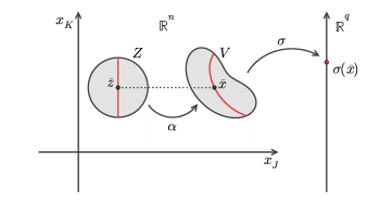
Figure 1: Graphical illustration of Lemma 2.1. The function $\alpha$ preserves the $K$ coordinates: $\alpha(z)=(\alpha_{J}(z),z_{K})$. On the other hand, since $\sigma(\alpha(z))=(z_{J},\lambda(z_{J}))$, points on the same “vertical line” (constant $J$ coordinates) are mapped by $\sigma\circ\alpha$ into a single point in $\mathbb{R}^{q}$.

In the next result we rewrite [3, Proposition 3.1] and [9, Proposition 2.2] in a suitable and more precise way. Despite the authors in these references comment, without adding any further argument, that this result is a special case of the constant rank theorem of [10], we consider that such a relation is not evident and the analysis is somewhat involved. We then give here a completely self-contained proof, using only the previous lemma.

Lemma 2.2

Let $\sigma:\mathbb{R}^{n}\to\mathbb{R}^{q}$ be a twice continuously differentiable function and suppose that $\sigma^{\prime}(x)$ has constant rank in a neighborhood of the point $\bar{x}\in\mathbb{R}^{n}$. Denote $D=\mathcal{N}(\sigma^{\prime}(\bar{x}))$ the nullspace of $\sigma^{\prime}(x)$. Then there exist neighborhoods $U$, $V$ of $\bar{x}$ and a twice continuously differentiable function $\phi:U\to V$ such that

$$\phi(\bar{x})=\bar{x},$$ (4a)

$$\phi^{\prime}(\bar{x})=I\in\mathbb{R}^{n\times n}\,(\mbox{the identity matrix}),$$ (4b)

$$\sigma(\phi(x+d))=\sigma(\phi(x))\mbox{ for all $x\in U$ and $d\in D$ such that $x+d\in U$.}$$ (4c)

In particular, $\sigma(\phi(\bar{x}+d))=\sigma(\bar{x})$ for all $d\in D$ such that $\bar{x}+d\in U$.

Proof. Let ${\rm rank}(\sigma^{\prime}(\bar{x}))=r$ and consider the function $\alpha:Z\to V$ defined in Lemma 2.1, which we know that has the form $\alpha(z)=(\alpha_{J}(z),z_{K})$. Define $\bar{z}=\alpha^{-1}(\bar{x})=(\xi(\bar{x}),\bar{x}_{K})$, $A=(\alpha^{\prime}(\bar{z}))^{-1}\in\mathbb{R}^{n\times n}$, $\gamma:\mathbb{R}^{n}\to\mathbb{R}^{n}$ by

$$\gamma(x)=A(x-\bar{x})+\bar{z},$$

$U=\gamma^{-1}(Z)$ and $\phi=\alpha\circ\gamma:U\to V$. Thus, we note immediately that $\phi(\bar{x})=\bar{x}$, giving (4a). Moreover, (4b) follows from

$$\phi^{\prime}(\bar{x})=\alpha^{\prime}(\gamma(\bar{x}))\gamma^{\prime}(\bar{x})=\alpha^{\prime}(\bar{z})\gamma^{\prime}(\bar{x})=I.$$

Finally, take $x\in U$ and $d\in D$ such that $x+d\in U$. Then,

$$\sigma^{\prime}(\alpha(\bar{z}))\alpha^{\prime}(\bar{z})Ad=\sigma^{\prime}(\bar{x})\alpha^{\prime}(\bar{z})Ad=\sigma^{\prime}(\bar{x})d=0.$$

On the other hand, since $\sigma(\alpha(z))=(z_{J},\lambda(z_{J}))$, we have

$$\sigma^{\prime}(\alpha(\bar{z}))\alpha^{\prime}(\bar{z})=\left(\begin{array}[]{cc}I&0\\ \lambda^{\prime}(\bar{z}_{J})&0\end{array}\right).$$

Therefore,

$$\left(\begin{array}[]{cc}I&0\\ \lambda^{\prime}(\bar{z}_{J})&0\end{array}\right)\left(\begin{array}[]{c}{[Ad]}_{J}\\ {[Ad]}_{K}\end{array}\right)=\left(\begin{array}[]{c}0\\ 0\end{array}\right),$$

which implies $[Ad]_{J}=0$ and hence,

$$\begin{array}[]{rcl}\sigma(\phi(x+d))&=&\sigma(\alpha(\gamma(x+d)))\vspace{.1cm}\\ &=&\sigma(\alpha(A(x-\bar{x}+d)+\bar{z}))\vspace{.1cm}\\ &=&([A(x-\bar{x}+d)+\bar{z}]_{J},\lambda([A(x-\bar{x}+d)+\bar{z}]_{J}))\vspace{.1cm}\\ &=&([A(x-\bar{x})+\bar{z}]_{J},\lambda([A(x-\bar{x})+\bar{z}]_{J}))\vspace{.1cm}\\ &=&([\gamma(x)]_{J},\lambda([\gamma(x)]_{J}))\vspace{.1cm}\\ &=&\sigma(\alpha(\gamma(x)))\vspace{.1cm}\\ &=&\sigma(\phi(x)),\end{array}$$

proving (4c).  

Lemma 2.2 is illustrated in Figure 2. The main role of the linear function $\gamma$ consists in mapping the points $x+d\in U$ into the “vertical line” in $Z$, making constant the function $d\mapsto\sigma(\phi(x+d))$.

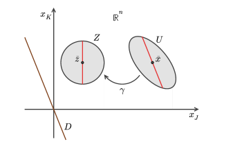
Figure 2: Illustration of Lemma 2.2. The linear function $\gamma$ maps the points $x+d\in U$ into the “vertical line” in $Z$, making constant the function $d\mapsto\sigma(\phi(x+d))$.

3 Second-order optimality conditions

In order to establish the results of this section, let us recall the three cones associated with problem (1), the tangent cone to $\Omega$ at $\bar{x}\in\Omega$

$$\mathcal{T}(\bar{x})=\left\{d\in\mathbb{R}^{n}\mid\exists\,(x^{k})\subset\Omega\mbox{, }(t_{k})\subset\mathbb{R}_{+}\mbox{ : }t_{k}\to 0\mbox{ and }\dfrac{x^{k}-\bar{x}}{t_{k}}\to d\right\},$$

the linearized cone

$$\mathcal{L}(\bar{x})=\{d\in\mathbb{R}^{n}\mid\nabla g_{i}(\bar{x})^{T}d\leq 0,\;i\in I_{g}(\bar{x}),\;\nabla h(\bar{x})^{T}d=0\}$$

and the strong critical cone

$$\mathcal{C}^{S}(\bar{x})=\{d\in\mathcal{L}(\bar{x})\mid\nabla f(\bar{x})^{T}d\leq 0\}.$$

First of all, note that if $\bar{x}$ is a KKT point for problem (1), then we can rewrite $\mathcal{C}^{S}(\bar{x})$ without using $\nabla f$ but instead, using the multipliers of $\bar{x}$. To be precise, if $(\bar{x},\mu,\lambda)\in\mathbb{R}^{n}\times\mathbb{R}^{m}_{+}\times\mathbb{R}^{p}$ is a primal-dual KKT point and $I_{g}^{+}(\bar{x})=\{i\in I_{g}(\bar{x})\mid\mu_{i}>0\}$, then

$$\mathcal{C}^{S}(\bar{x})=\{d\in\mathcal{L}(\bar{x})\mid\nabla g_{i}(\bar{x})^{T}d=0,\ i\in I_{g}^{+}(\bar{x})\}.$$

This follows immediately from the fact that

$$\nabla f(\bar{x})^{T}d=-\sum_{i\in I_{g}(\bar{x})}\mu_{i}\nabla g_{i}(\bar{x})^{T}d$$

for all $d\in\mathcal{L}(\bar{x})$.

Definition 3.1

Let $\bar{x}$ be a KKT point for problem (1). We say that $\bar{x}$ fulfills the strong second-order optimality necessary condition (SSONC) if for every multiplier vector $(\mu,\lambda)\in\mathbb{R}_{+}^{m}\times\mathbb{R}^{p}$ associated with $\bar{x}$ we have

$$d^{T}\nabla^{2}_{xx}\ell(\bar{x},\mu,\lambda)d\geq 0$$

for all $d\in\mathcal{C}^{S}(\bar{x})$.

In the example below, we see that MFCQ is not a second-order constraint qualification (and hence, none of CQs implied by MFCQ).

Example 3.2

Consider the problem in $\mathbb{R}^{2}$ given by

$$\begin{array}[]{cl}\displaystyle\mathop{\rm minimize}&f(x)=x_{2}\\ {\rm subject\ to}&g_{1}(x)=x_{1}^{2}+(x_{2}-1)^{2}-1\leq 0,\\ &g_{2}(x)=1-x_{1}^{2}-(x_{2}+1)^{2}\leq 0.\end{array}$$

It is easy to see that $x^{*}=\left(\begin{array}[]{c}0\\ 0\end{array}\right)$ is the global solution of the problem and that MFCQ holds at $x^{*}$. Indeed, $(x_{2}-1)^{2}\leq x_{1}^{2}+(x_{2}-1)^{2}\leq 1$ implies that $x_{2}\geq 0$. Moreover, we have

$$\nabla g_{1}(x^{*})=\nabla g_{2}(x^{*})=\left(\begin{array}[]{c}0\\ -2\end{array}\right),$$

which means that there exists $d\in\mathbb{R}^{2}$ such that $\nabla g_{i}(x^{*})^{T}d<0$.

On the other hand,

$$\nabla f(x^{*})+\mu_{1}\nabla g_{1}(x^{*})+\mu_{2}\nabla g_{2}(x^{*})=\left(\begin{array}[]{c}0\\ 1\end{array}\right)+\left(\begin{array}[]{c}0\\ -2\mu_{1}-2\mu_{2}\end{array}\right),$$

so that the Lagrange multipliers satisfy $2(\mu_{1}+\mu_{2})=1$. The critical cone is

$$\mathcal{C}^{S}(x^{*})=\{d\in\mathbb{R}^{2}\mid d_{2}=0\}$$

and the Lagrangian Hessian at this point is

$$\nabla^{2}f(x^{*})+\mu_{1}\nabla^{2}g_{1}(x^{*})+\mu_{2}\nabla^{2}g_{2}(x^{*})=2(\mu_{1}-\mu_{2})I.$$

Thus, taking $\mu_{1}<\mu_{2}$ and $d\in\mathcal{C}^{S}(x^{*})\setminus\{0\}$, we have

$$d^{T}\left(\nabla^{2}f(x^{*})+\mu_{1}\nabla^{2}g_{1}(x^{*})+\mu_{2}\nabla^{2}g_{2}(x^{*})\right)d=2(\mu_{1}-\mu_{2})d_{1}^{2}<0.$$

The result below shows, in particular, that (under RCRCQ) any linearized feasible direction $\bar{d}\in\mathcal{L}(\bar{x})$ is the velocity vector of a feasible arc at $\bar{x}\in\Omega$, which will allow us to derive ACQ directly from RCRCQ (without following the path of Figure 2 of [6]).

Proposition 3.3

Suppose that the relaxed constant rank constraint qualification holds at $\bar{x}\in\Omega$. Given $\bar{d}\in\mathcal{L}(\bar{x})$, define $J=\{j\in I_{g}(\bar{x})\mid\nabla g_{j}(\bar{x})^{T}\bar{d}=0\}$. Then there exists a twice continuously differentiable arc $\zeta:(-\delta,\delta)\to\mathbb{R}^{n}$ such that

$$\zeta(0)=\bar{x},\;\zeta^{\prime}(0)=\bar{d},$$ (5a)

$$g_{j}(\zeta(t))=0\mbox{ for all $t\in(-\delta,\delta)$ and $j\in J$,}$$ (5b)

$$g_{j}(\zeta(t))\leq 0\mbox{ for all $t\in(-\delta,\delta)$ and $j\notin I_{g}(\bar{x})$,}$$ (5c)

$$g_{j}(\zeta(t))\leq 0\mbox{ for all $t\in[0,\delta)$ and $j\in I_{g}(\bar{x})\setminus J$,}$$ (5d)

$$h(\zeta(t))=0\mbox{ for all $t\in(-\delta,\delta)$.}$$ (5e)

In particular, $\zeta(t)\in\Omega$ for all $t\in[0,\delta)$ and hence, $\bar{d}\in\mathcal{T}(\bar{x})$.

Proof. Define $\sigma:\mathbb{R}^{n}\to\mathbb{R}^{|J|+p}$ defined by $\sigma(x)=(g_{J}(x),h(x))$. By the constraint qualification, $\sigma^{\prime}(x)$ has constant rank in a neighborhood of $\bar{x}$. Therefore, applying Lemma 2.2 we conclude that there exist neighborhoods $U$, $V$ of $\bar{x}$ and a twice continuously differentiable function $\phi:U\to V$ such that $\phi(\bar{x})=\bar{x}$, $\phi^{\prime}(\bar{x})=I\in\mathbb{R}^{n\times n}$ and

$$\sigma(\phi(\bar{x}+d))=\sigma(\bar{x})$$ (6)

for all $d\in\mathcal{N}(\sigma^{\prime}(\bar{x}))$ such that $\bar{x}+d\in U$. Consider $\delta>0$ such that $\bar{x}+t\bar{d}\in U$ for all $t\in(-\delta,\delta)$ and define $\zeta:(-\delta,\delta)\to\mathbb{R}^{n}$ by $\zeta(t)=\phi(\bar{x}+t\bar{d})$. Thus,

$$\zeta(0)=\phi(\bar{x})=\bar{x}\quad\mbox{and}\quad\zeta^{\prime}(0)=\phi^{\prime}(\bar{x})\bar{d}=\bar{d},$$

giving (5a). Furthermore, since $\bar{d}\in\mathcal{N}(\sigma^{\prime}(\bar{x}))$, we have

$$\sigma(\zeta(t))=\sigma(\phi(\bar{x}+t\bar{d}))=\sigma(\bar{x})=0,$$

proving (5b) and (5e). The continuity of $g$ immediately gives (5c). Now, given $j\in I_{g}(\bar{x})\setminus J$, we have $\nabla g_{j}(\bar{x})^{T}\bar{d}<0$ and then

$$(g_{j}\circ\zeta)^{\prime}(0)=g_{j}^{\prime}(\zeta(0))\zeta^{\prime}(0)=g_{j}^{\prime}(\bar{x})\bar{d}=\nabla g_{j}(\bar{x})^{T}\bar{d}<0,$$

giving $g_{j}(\zeta(t))\leq g_{j}(\zeta(0))=0$ for all $t\geq 0$ sufficiently small. By reducing $\delta$ if necessary, we obtain (5d). Finally, taking $(t_{k})\subset(0,\delta)$ with $t_{k}\to 0$, we have

$$\dfrac{\zeta(t_{k})-\bar{x}}{t_{k}}\to\bar{d},$$

which means that $\bar{d}\in\mathcal{T}(\bar{x})$.  

We point out that Proposition 3.3 generalizes [3, Proposition 3.2] and [9, Proposition 2.3] in three aspects. First, we assume the weaker hypothesis RCRCQ instead of CRCQ. Second, the arc $\zeta$ we constructed here is defined on the whole interval $(-\delta,\delta)$, while in the mentioned references the domain is an interval of the form $(0,\delta)$ and hence they have only the right-hand derivative. Finally we proved stronger smoothness of the arc $\zeta$ than in the referred references: we shall need second-order differentiability to establish second-order optimality conditions.

We should also mention that [12, Lemma 2.5] provides an arc with similar properties. However, the relation in (5b) is valid for the bigger set $J$. Moreover, they consider a direction in the relative interior of the critical cone, while here we take an arbitrary direction in the linearized cone.

A first (and immediate) consequence of Proposition 3.3 is given next.

Corollary 3.4

Suppose that RCRCQ holds at $\bar{x}\in\Omega$. Then $\mathcal{L}(\bar{x})\subset\mathcal{T}(\bar{x})$, which in turn implies ACQ.

Now we derive the main result of the paper as another consequence of Proposition 3.3, with a quite elementary proof.

Theorem 3.5

Let $x^{*}\in\Omega$ be a local minimizer of the problem (1) satisfying RCRCQ. Then SSONC (Definition 3.1) holds at $x^{*}$.

Proof. Since $\mathcal{C}^{S}(x^{*})\subset\mathcal{L}(x^{*})$, Proposition 3.3 ensures the existence of a twice continuously differentiable arc $\zeta:(-\delta,\delta)\to\mathbb{R}^{n}$ such that $\zeta(0)=x^{*}$, $\zeta^{\prime}(0)=d$, $\zeta(t)\in\Omega$ for all $t\in[0,\delta)$ and $g_{j}(\zeta(t))=0$ for all $t\in(-\delta,\delta)$ and $j\in I_{g}^{+}(x^{*})$ (note that $I_{g}^{+}(x^{*})\subset J$). Define $\beta:(-\delta,\delta)\to\mathbb{R}$ by $\beta(t)=f(\zeta(t))$. Since $x^{*}$ satisfies the KKT conditions, let $(\mu,\lambda)\in\mathbb{R}^{m}_{+}\times\mathbb{R}^{p}$ be an arbitrary multiplier vector associated with it. Then

$$\nabla f(x^{*})+\sum_{j\in I_{g}^{+}(x^{*})}\mu_{j}\nabla g_{j}(x^{*})+\sum_{i=1}^{p}\lambda_{i}\nabla h_{i}(x^{*})=0$$ (7)

and consequently $\beta^{\prime}(0)=\nabla f(x^{*})^{T}d=0$. Moreover, $x^{*}$ is a local minimizer of (1) and hence $\beta(0)\leq\beta(t)$ for all $t\geq 0$ sufficiently small. Therefore,

$$d^{T}\nabla^{2}f(x^{*})d+\nabla f(x^{*})^{T}\zeta^{\prime\prime}(0)=\beta^{\prime\prime}(0)\geq 0.$$ (8)

On the other hand, we have

$$d^{T}\nabla^{2}g_{j}(x^{*})d+\nabla g_{j}(x^{*})^{T}\zeta^{\prime\prime}(0)=(g_{j}\circ\zeta)^{\prime\prime}(0)=0.$$ (9)

for $j\in I_{g}^{+}(x^{*})$ and

$$d^{T}\nabla^{2}h_{i}(x^{*})d+\nabla h_{i}(x^{*})^{T}\zeta^{\prime\prime}(0)=(h_{i}\circ\zeta)^{\prime\prime}(0)=0.$$ (10)

for $i=1,\ldots,p$. Thus, multiplying (9) by $\mu_{j}$, (10) by $\lambda_{i}$ and summing the resulting expressions over $j\in I_{g}^{+}(x^{*})$ and $i=1,\ldots,p$ together with (8), we obtain the desired result in view of (7).  

It should be noted that, although RCRCQ is weaker than LICQ and CRCQ, it is not a necessary assumption for strong second-order condition, as we see in the next example.

Example 3.6

Consider the two dimensional problem

$$\begin{array}[]{cl}\displaystyle\mathop{\rm minimize}&f(x)=x_{2}\\ {\rm subject\ to}&g_{1}(x)=x_{1}^{2}-x_{2}\leq 0,\\ &g_{2}(x)=-x_{2}\leq 0.\end{array}$$

We have that $x^{*}=\left(\begin{array}[]{c}0\\ 0\end{array}\right)$ is the global solution of the problem. Moreover, since

$$\nabla g_{1}(x^{*})=\nabla g_{2}(x^{*})=\left(\begin{array}[]{c}0\\ -1\end{array}\right),$$

MFCQ holds at $x^{*}$. Thus, there exist Lagrange multipliers and they must satisfy

$$\left(\begin{array}[]{c}0\\ 1-\mu_{1}-\mu_{2}\end{array}\right)=\nabla f(x^{*})+\mu_{1}\nabla g_{1}(x^{*})+\mu_{2}\nabla g_{2}(x^{*})=0,$$

which means that $\mu_{1}+\mu_{2}=1$. The critical cone is

$$\mathcal{C}^{S}(x^{*})=\{d\in\mathbb{R}^{2}\mid d_{2}=0\}$$

and the Lagrangian Hessian at $x^{*}$ is

$$\nabla^{2}f(x^{*})+\mu_{1}\nabla^{2}g_{1}(x^{*})+\mu_{2}\nabla^{2}g_{2}(x^{*})=2\left(\begin{array}[]{cc}\mu_{1}&0\\ 0&0\end{array}\right),$$

so that SSONC is satisfied at this point. On the other hand, the vectors $\nabla g_{1}(x)=\left(\begin{array}[]{c}2x_{1}\\ -1\end{array}\right)$ and $\nabla g_{2}(x)=\left(\begin{array}[]{c}0\\ -1\end{array}\right)$ do not have the same rank for every $x$ in a neighborhood of $x^{*}$, that is, RCRCQ does not hold at $x^{*}$.

In view of the example above, it is natural to ask whether there is a constraint qualification, weaker than RCRCQ, that implies SSONC. In [2, Theorem 3.2] the authors establish SSONC under an Abadie-type assumption. Despite their hypothesis is weaker than RCRCQ, it is not a constraint qualification. So, the existence of Lagrange multipliers is not guaranteed by such an assumption. On the other hand, the second-order cone-continuity property (CCP2) [5] is a constraint qualification implied by RCRCQ. However, it ensures only the weak second-order optimality condition (WSONC) [5, Theorem 4.2]. In this reference the authors also define strong CCP2 (SCCP2) and prove that SSONC is valid under this CQ [5, Theorem 4.16], but RCRCQ and SCCP2 are independent of each other. Both CCP2 and SCCP2 are constraint qualifications associated to a second-order sequential optimality condition (AKKT2) related to the convergence of optimization algorithms. Indeed, note that Example 3.2, together with the relations among all established CQs, allows us to conclude that RCRCQ is the weakest constraint qualification that ensures strong second-order necessary condition.

4 Conclusions

In this short note we have discussed and established the first- and second-order optimality conditions for nonlinear programming, assuming the relaxed constant rank constraint qualification, through a quite elementary approach. The only prerequisite used here to establish auxiliary results is the classical and well-known inverse function theorem. We also have generalized results of [3, 9] assuming RCRCQ instead of CRCQ and presented examples and discussions that allow us to conclude that RCRCQ is the weakest CQ ensuring SSONC.

References

[1]
Abadie, J.: On the Kuhn-Tucker Theorem.
In: J. Abadie (ed.) Nonlinear Programming, pp. 19–36. North Holland,
Amsterdam (1967)
[2]
Andreani, R., Behling, R., Haeser, G., Silva, P.J.S.: On second-order
optimality conditions in nonlinear optimization.
Optim. Methods Softw. 32, 22–38 (2017).
DOI 10.1080/10556788.2016.1188926
[3]
Andreani, R., Echagüe, C.E., Schuverdt, M.L.: Constant-rank condition and
second-order constraint qualification.
J. Optim. Theory Appl. 146, 255–266 (2010).
DOI 10.1007/s10957-010-9671-8
[4]
Andreani, R., Haeser, G., Ramos, A., Silva, P.J.S.: A relaxed constant positive
linear dependence constraint qualification and applications.
Math. Program. 135, 255–273 (2012)
[5]
Andreani, R., Haeser, G., Ramos, A., Silva, P.J.S.: A second-order sequential
optimality condition associated to the convergence of optimization
algorithms.
IMA J. Numer. Anal. 37(4), 1902–1929 (2017)
[6]
Andreani, R., Martínez, J.M., Ramos, A., Silva, P.J.S.: A cone-continuity
constraint qualification and algorithmic consequences.
SIAM J. Optim. 26(1), 96–110 (2016)
[7]
Andreani, R., Martínez, J.M., Schuverdt, M.L.: On the relation between
constant positive linear dependence condition and quasinormality constraint
qualification.
J. Optim. Theory Appl. 125(2), 473–485 (2005)
[8]
Guignard, M.: Generalized Kuhn-Tucker conditions for mathematical
programming problems in a Banach space.
SIAM J. Control 7, 232–241 (1969)
[9]
Janin, R.: Directional derivative of the marginal function in nonlinear
programming.
In: A.V. Fiacco (ed.) Sensitivity, Stability and Parametric Analysis,
vol. 21, pp. 110–126. Math. Program. Stud., Berlin Heidelberg (1984).
DOI 10.1007/BFb0121214
[10]
Malliavin, P.: Géométrie différentielle intrinsèque.
Herman, Paris (1972)
[11]
Mangasarian, O.L., Fromovitz, S.: The fritz john necessary optimality
conditions in the presence of equality and inequality constraints.
J. Math. Anal. Appl. 17, 37–47 (1967)
[12]
Minchenko, L., Leschov, A.: On strong and weak second-order necessary
optimality conditions for nonlinear programming.
Optimization 65, 1693–1702 (2016).
DOI 10.1080/02331934.2016.1179300
[13]
Minchenko, L., Stakhovski, S.: On relaxed constant rank regularity condition in
mathematical programming.
Optimization 60, 429–440 (2011).
DOI 10.1080/02331930902971377
[14]
Minchenko, L., Stakhovski, S.: Parametric nonlinear programming problems under
the relaxed constant rank condition.
SIAM J. Optim. 21, 314–332 (2011).
DOI 10.1137/090761318
[15]
Qi, L., Wei, Z.: On the constant positive linear dependence condition and its
application to SQP methods.
SIAM J. Optim. 10(4), 963–981 (2000)