Self-Supervised Information Bottleneck for Deep Multi-View Subspace Clustering

Abstract

In this paper, we explore the problem of deep multi-view subspace clustering framework from an information-theoretic point of view. We extend the traditional information bottleneck principle to learn common information among different views in a self-supervised manner, and accordingly establish a new framework called Self-supervised Information Bottleneck based Multi-view Subspace Clustering (SIB-MSC). Inheriting the advantages from information bottleneck, SIB-MSC can learn a latent space for each view to capture common information among the latent representations of different views by removing superfluous information from the view itself while retaining sufficient information for the latent representations of other views. Actually, the latent representation of each view provides a kind of self-supervised signal for training the latent representations of other views. Moreover, SIB-MSC attempts to learn the other latent space for each view to capture the view-specific information by introducing mutual information based regularization terms, so as to further improve the performance of multi-view subspace clustering. To the best of our knowledge, this is the first work to explore information bottleneck for multi-view subspace clustering. Extensive experiments on real-world multi-view data demonstrate that our method achieves superior performance over the related state-of-the-art methods.

1 Introduction

Multi-view subspace clustering aims to discover the underlying subspace structures of data by fusing different view information. A popular strategy is to take advantage of a linear model to learn an affinity matrix for each view, and then build a consensus graph based on these affinity matrices  Günnemann et al. (2012). Following this line, many approaches have been proposed in the past decade. For instance, Gao et al. (2015) performs subspace clustering on each view, and uses a common cluster structure to make sure the consistence among different views. Cao et al. (2015) employs the Hilbert Schmidt Independence Criterion (HSIC) Gretton et al. (2005) to explore the complementary information of different views, and obtains diverse subspace representations. Zhang et al. (2015) presents a low-rank tensor constraint to explore the complementary information from multiple views, which can capture the high order correlations of multi-view data. Furthermore, Zhang et al. (2017) attempts to seek a latent representation to well reconstruct the data of all views, and perform clustering based on the learned latent representation. Kang et al. (2020) proposes to learn a smaller graph between the raw data points and the generated anchors for each view, and then designs an integration mechanism to merge those graphs, making the eigen-value decomposition accelerated significantly. However, all of these methods use linear models to model multi-view data, thus often failing in handling data with complex (often nonlinear) structures.

In recent years, with the development of deep learning techniques, a few deep learning based methods have been gradually proposed for multi-view subspace clustering Abavisani and Patel (2018); Zhu et al. (2019); Zhang et al. (2020), which mainly aim to leverage deep learning to non-linearly map data into latent spaces for capturing complementary information or diverse information among different views. The representative works including Deep Multimodal Subspace Clustering networks (DMSC) Abavisani and Patel (2018), Multi-View Deep Subspace Clustering Networks (MvDSCN) Zhu et al. (2019), generalized Latent Multi-View Subspace Clustering (gLMSC) Zhang et al. (2020). Because of the powerful representation ability of deep learning, these methods achieve promising performance.

Recently, information bottleneck has attracted increasing attention in the machine learning community Motiian et al. (2016); Federici et al. (2020); Wan et al. (2021); Yu et al. (2021). Information bottleneck is an information theoretic principle that can learn a minimal sufficient representation for downstream prediction tasks Tishby et al. (2000). So far, information bottleneck has been widely applied to representation learning Wan et al. (2021), graph learning Wu et al. (2020), visual recognition Motiian et al. (2016), etc. However, there is few work to explore information bottleneck for deep multi-view subspace clustering.

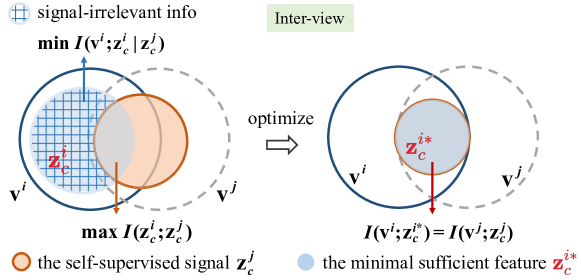
Figure 1: High-level takeaways for our self-supervised information bottleneck.

In light of this, we propose a new deep multi-view subspace clustering framework in this paper, called Self-supervised Information Bottleneck based Multi-view Subspace Clustering (SIB-MSC). In order to learn the view-common information, we extend information bottleneck to learn the latent space of each view by removing superfluous information from the view itself while retaining sufficient information for the latent representations of other views. As shown in Figure 1, taking the latent representation $\mathbf{z}_{c}^{j}$ extracted from the $j$-th view as an anchor, we expect that $\mathbf{z}_{c}^{i}$ can remove superfluous information from the original input $\mathbf{v}^{i}$ of the $i$-th view by minimizing the conditional mutual information $I(\mathbf{v}^{i};\mathbf{z}_{c}^{i}|\mathbf{z}_{c}^{j})$ while preserving sufficient information for $\mathbf{z}_{c}^{j}$ by maximizing the mutual information between $\mathbf{z}_{c}^{i}$ and $\mathbf{z}_{c}^{j}$. Actually, the latent representation $\mathbf{z}_{c}^{j}$ serves as a self-supervised signal to guide the learning of the latent representation $\mathbf{z}_{c}^{i}$. Moreover, we attempt to learn view-specific information for each view by imposing mutual information based constraints to further improve the representation ability of the model. After that, the affinity matrices based on the minimal sufficient view-common representations is taken as the input to spectral clustering.

In summary, our contributions are four-fold:

• We propose an information bottleneck based framework for deep multi-view subspace clustering. To the best of our knowledge, this is the first work to explore information bottleneck for multi-view subspace clustering.

• We put forward to learn the minimal sufficient latent representation for each view with the guidance of self-supervised information bottleneck, which can obtain common information among different views.

• We present mutual information based constraints to capture a view-specific space for each view to be complementary to the view-common space, and well reconstruct the samples, such that the performance can be further improved.

• Extensive experiments on multi-view data verify the effectiveness of our proposed model. Moreover, our model achieves superior performance over the existing deep multi-view subspace clustering algorithms.

2 Related Work

In this section, we review some related works on deep multi-view subspace clustering and information bottleneck based representation learning.

Deep Multi-View Subspace Clustering.

Deep learning has demonstrated the powerful representation ability in various learning tasks. In recent years, there are a few works which attempt to leverage deep learning to solve the problem of multi-view subspace clustering Abavisani and Patel (2018); Zhu et al. (2019); Zhang et al. (2020). DMSC Abavisani and Patel (2018) takes advantage of deep learning to investigate the early, intermediate and late fusion strategies to learn a latent space which is used to discover the subspace structures of the data. Zhu et al. (2019) proposes to learn a view-specific self-representation matrix for each view and a common self-representation matrix for all views. Then, the learned common self-representation matrix is used to perform spectral clustering Ng et al. (2002). gLMSC Zhang et al. (2020) aims to integrate multi-view inputs into a comprehensive latent representation which can encode complementary information from different views and well capture the underlying subspace structure. Different from these works, we focus on studying the problem of deep multi-view subspace clustering from an information-theoretic point of view.

Representation Learning with Information Bottleneck.

The information bottleneck principle can learn a robust representation by removing information from the input that is not relevant to a given task. Tishby et al. (2000). Because of its effectiveness, information bottleneck has been successfully applied to representation learning Motiian et al. (2016); Alemi et al. (2017); Federici et al. (2020); Wan et al. (2021); Yu et al. (2021). Motiian et al. (2016) extends the information bottleneck principle to leverage an auxiliary data view during training for learning a better visual classifier. VIB  Alemi et al. (2017) is a variational approximation to the information bottleneck, which can parameterize the information bottleneck method using a neural network. MIB Federici et al. (2020) is proposed to minimize the mutual information between two different views to reduce the redundant information across them, where the original input is regarded as a self-supervised signal. Wan et al. (2021) utilizes the information bottleneck principle to remove the superfluous information from the multi-view data. Yu et al. (2021) applies information bottleneck to identify the maximally informative yet compressive subgraph for subgraph recognition. As aforementioned, we attempt to extend the information bottleneck principle to deep multi-view subspace clustering, motivated by these methods.

3 The Proposed Method

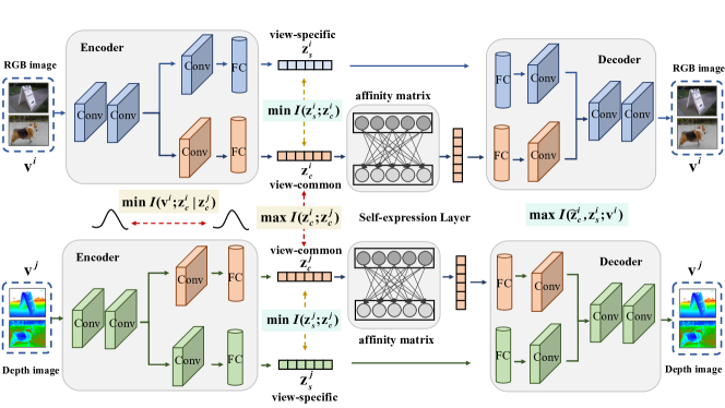
Figure 2: Illustration of the overall architecture. SIB-MSC extends information bottleneck to learn a latent space $\mathbf{z}_{c}^{i}$ for each the $i-$th view for capturing view-common information among different views. Taking the latent representation $\mathbf{z}_{c}^{j}$ as an anchor, we expect to eliminate the useless information from the original view $i$ by minimizing $I(\mathbf{v}^{i};\mathbf{z}_{c}^{i}|\mathbf{z}_{c}^{j})$ while preserving sufficient information for $\mathbf{z}_{c}^{j}$ by maximizing $I(\mathbf{z}_{c}^{i};\mathbf{z}_{c}^{j})$. Here, the latent representation $\mathbf{z}_{c}^{j}$ plays a role of self-supervision. Moreover, the view-specific feature $\mathbf{z}_{s}^{i}$ is extracted to maintain the complementary information, by minimizing $I(\mathbf{z}_{s}^{i};\mathbf{z}_{c}^{i})$ to disentangle from $\mathbf{z}_{c}^{i}$ and maximizing $I(\widetilde{\mathbf{z}}_{c}^{i},\mathbf{z}_{s}^{i};\mathbf{v}^{i})$ to achieve jointly informative to the original inputs, such that the performance of multi-view subspace learning can be further improved. After that, the affinity matrices obtained based on the view-common representations are taken as the input to spectral clustering.

In this section, we will elaborate the details of the proposed deep multi-view subspace clustering framework, as shown in Figure 2. For better clarification, we first give some notations.

Notation Statement.

Suppose that we have $m$ views, let $\mathbf{V}=\{\mathbf{V}^{1},\cdots,\mathbf{V}^{m}\}$ be the input samples, where $\mathbf{V}^{i}=\{\mathbf{v}_{1}^{i},\mathbf{v}_{2}^{i},\cdots,\mathbf{v}_{n}^{i}\}\in\mathbb{R}^{n\times d_{i}}$ denotes the samples of the $i$-th view, $d_{i}$ denotes the feature dimension of the $i$-th view, and $n$ is the number of samples. $\mathbf{v}^{i}_{k}$ denotes the $k$-th sample of view $i$. For writing conveniently, we use the notation $\mathbf{v}^{i}$ to take place of $\mathbf{v}^{i}_{k}$ throughout the paper. For each sample $\mathbf{v}^{i}$, we extract two kinds of features: a view-common feature $\mathbf{z}_{c}^{i}\in\mathbb{R}^{d}$ and a view-specific feature $\mathbf{z}_{s}^{i}\in\mathbb{R}^{d}$. Given three random variables, ${X}$, ${Y}$ and ${Z}$, we measure the mutual dependence between $X$ and $Y$ with the aid of mutual information $I({X};{Y})$. In addition, we can leverage conditional mutual information $I({X};{Y}|{Z})$ to measure the amount of information that $Y$ can capture from $X$ that is irrelevant to $Z$.

3.1 Learning View-Common via Information Bottleneck

To capture the view-common information, we extend information bottleneck to reach this goal, where the latent representation of each view is learnt by discarding useless information from the view that is not relevant to other views. In this paper, we first consider the case of two views, in order to simplify the statement. It is easily extended to the general case which has more than two views.

As shown in Figure 2, to make the learnt $\mathbf{z}_{c}^{i}$ and $\mathbf{z}_{c}^{j}$ contain the common information as much as possible, we take $\mathbf{z}_{c}^{i}$ and $\mathbf{z}_{c}^{j}$ as self-supervised signals to guide the learning of each other, respectively. Here, we take $\mathbf{z}_{c}^{j}$ as an example to show how to guide the learning of $\mathbf{z}_{c}^{i}$. The learning process of $\mathbf{z}_{c}^{j}$ is the same. We first decompose the mutual information between $\mathbf{v}^{i}$ and $\mathbf{z}_{c}^{i}$ into two components:

$$I(\mathbf{v}^{i};\mathbf{z}_{c}^{i})=\underbrace{I(\mathbf{v}^{i};\mathbf{z}_{c}^{i}|\mathbf{z}_{c}^{j})}_{\rm signal-irrelevant}+\underbrace{I(\mathbf{z}_{c}^{i};\mathbf{z}_{c}^{j})}_{\rm signal-relevant},$$ (1)

where the conditional mutual information $I(\mathbf{v}^{i};\mathbf{z}_{c}^{i}|\mathbf{z}_{c}^{j})$ represents the information that $\mathbf{z}_{c}^{i}$ can capture from $\mathbf{v}^{i}$ and is not relevant to $\mathbf{z}_{c}^{j}$, i.e., the superfluous information. $I(\mathbf{z}_{c}^{i};\mathbf{z}_{c}^{j})$ measures how much information of $\mathbf{z}_{c}^{j}$ is accessible from $\mathbf{z}_{c}^{i}$.

In Eq. (1), we minimize the signal-irrelevant part to discard the superfluous information, and maximize the signal-relevant part to encourage $\mathbf{z}_{c}^{i}$ to be sufficient for $\mathbf{z}_{c}^{j}$. Therefore, we propose to minimize the following loss function to learn the minimal sufficient feature $\mathbf{z}_{c}^{i}$ as:

$$\mathcal{L}_{c}^{i}=-I(\mathbf{z}_{c}^{i};\mathbf{z}_{c}^{j})+\lambda_{i}I(\mathbf{v}^{i};\mathbf{z}_{c}^{i}|\mathbf{z}_{c}^{j}),$$ (2)

where $\lambda_{i}$ is the Lagrangian multiplier introduced by the information constraint.

Since it is difficult to directly handle the conditional mutual information, we can conduct the transformation based on the chain rule of the conditional mutual information as:

$$I(\mathbf{v}^{i};\mathbf{z}_{c}^{i}|\mathbf{z}_{c}^{j})=I(\mathbf{v}^{i};\mathbf{z}_{c}^{i},\mathbf{z}_{c}^{j})-I(\mathbf{v}^{i};\mathbf{z}_{c}^{j})$$

$$=I(\mathbf{v}^{i};\mathbf{z}_{c}^{i})+I(\mathbf{z}_{c}^{j};\mathbf{v}^{i}|\mathbf{z}_{c}^{i})-I(\mathbf{v}^{i};\mathbf{z}_{c}^{j})$$

$$=I(\mathbf{v}^{i};\mathbf{z}_{c}^{i})-I(\mathbf{v}^{i};\mathbf{z}_{c}^{j}).$$ (3)

Based on Eq. (3.1), we can rewrite Eq. (2) as:

$$\mathcal{L}_{c}^{i} =-I(\mathbf{z}_{c}^{i};\mathbf{z}_{c}^{j})+\lambda_{i}I(\mathbf{v}^{i};\mathbf{z}_{c}^{i}|\mathbf{z}_{c}^{j})$$

$$=- I(\mathbf{z}_{c}^{i};\mathbf{z}_{c}^{j})+\lambda_{i}(I(\mathbf{v}^{i};\mathbf{z}_{c}^{i})-I(\mathbf{z}_{c}^{j};\mathbf{v}^{i})).$$ (4)

Let us first study the cross-view mutual information maximization $I(\mathbf{z}_{c}^{j};\mathbf{v}^{i})$. Considering the fact that $\mathbf{v}^{i}$ is over-informative for subspace clustering concerning more about the structure information, we relieve $\mathbf{v}^{j}$ to $\mathbf{h}^{j}$ which is the exact feature the encoder extracted before splitting into two parts, thus we have $I(\mathbf{z}_{c}^{j};\mathbf{v}^{i})\geq I(\mathbf{z}_{c}^{j};\mathbf{h}^{i})$.

Jointly considering the $i$-th and $j$-th views, we can obtain the loss function for learning the view-common latent space:

$$\mathcal{L}_{c}= \mathcal{L}_{c}^{i}+\mathcal{L}_{c}^{j}$$

$$= -2*I(\mathbf{z}_{c}^{i};\mathbf{z}_{c}^{j})+\lambda_{i}(I(\mathbf{v}^{i};\mathbf{z}_{c}^{i})-I(\mathbf{z}_{c}^{j};\mathbf{v}^{i}))$$

$$+\lambda_{j}(I(\mathbf{v}^{j};\mathbf{z}_{c}^{j})-I(\mathbf{z}_{c}^{i};\mathbf{v}^{j}))$$

$$\leq -2*I(\mathbf{z}_{c}^{i};\mathbf{z}_{c}^{j})-(\lambda_{i}I(\mathbf{z}_{c}^{j};\mathbf{h}^{i})+\lambda_{j}I(\mathbf{z}_{c}^{i};\mathbf{h}^{j}))$$

$$+(\lambda_{i}I(\mathbf{v}^{i};\mathbf{z}_{c}^{i})+\lambda_{j}I(\mathbf{v}^{j};\mathbf{z}_{c}^{j})).$$ (5)

where we can divide the above loss function into three types of terms as $\mathcal{L}_{c}^{dis}=-2*I(\mathbf{z}_{c}^{i};\mathbf{z}_{c}^{j})$, $\mathcal{L}_{c}^{cmi}=-(\lambda_{i}I(\mathbf{z}_{c}^{j};\mathbf{h}^{i})+\lambda_{j}I(\mathbf{z}_{c}^{i};\mathbf{h}^{j}))$, $\mathcal{L}_{c}^{mkl}=\lambda_{i}I(\mathbf{v}^{i};\mathbf{z}_{c}^{i})+\lambda_{j}I(\mathbf{v}^{j};\mathbf{z}_{c}^{j})$. We denote these notations, with the purpose of performing the ablation study in the experiment conveniently.

Thus, minimizing $\mathcal{L}_{c}$ can be relaxed to minimize its upper bound, i.e., the right part of the inequality sign. Since it is difficult to directly optimize Eq. (3.1) due to involving several mutual information terms, we attempt to seek an approximate solution to Eq. (3.1). Here we only present our formulation for view $i$, as the one for view $j$ is analogous. We first consider the cross-view mutual information maximization:

$$I(\mathbf{z}_{c}^{j};\mathbf{h}^{i})=D_{KL}[p(\mathbf{z}_{c}^{j},\mathbf{h}^{i})||p(\mathbf{z}_{c}^{j})p(\mathbf{h}^{i})].$$ (6)

As the essence of mutual information is KL divergence and the maximization of KL-divergence is divergent, we instead seek for the convergent Jensen-Shannon MI estimator as in  Nowozin et al. (2016), thus a tractable estimation of $I(\mathbf{z}_{c}^{j};\mathbf{h}^{i})$ can be defined as:

$$\max\quad \mathbb{E}_{(\mathbf{z}_{c}^{j};\mathbf{h}^{i})}[\log\mathrm{D}(\mathbf{z}_{c}^{j},\mathbf{h}^{i})]$$

$$+\mathbb{E}_{(\mathbf{z}_{c}^{j};\mathbf{\hat{h}}^{i})}[\log(1-\mathrm{D}(\mathbf{z}_{c}^{j},\mathbf{\hat{h}}^{i}))],$$ (7)

where the feature $\mathbf{z}_{c}^{j}$ serves as the anchor, and the features $\mathbf{z}_{c}^{j}$ and $\mathbf{h}^{i}$ originated from view $i$ of the same example are regarded as a positive pair. $\mathbf{\hat{h}}^{i}$ denotes random sampled negative input from view $i$, and $\mathrm{D}$ indicates the discriminator to estimate the probability of the input pair.

Similarly, the mutual information maximization term $I(\mathbf{z}_{c}^{i};\mathbf{z}_{c}^{j})$ can be also tractable by replacing $\mathbf{h}^{i}$ wth $\mathbf{z}_{c}^{i}$ in Eq. (6).

As for the mutual information minimization term $I(\mathbf{v}^{i};\mathbf{z}_{c}^{i})$, let $q(\mathbf{z}_{c}^{i})$ be a variational approximation of $p(\mathbf{z}_{c}^{i})$, with $D_{KL}[p(\mathbf{z}_{c}^{i}),q(\mathbf{z}_{c}^{i})]\geq 0\Rightarrow\int p(\mathbf{z}_{c}^{i})\log p(\mathbf{z}_{c}^{i})d\mathbf{z}_{c}^{i}\geq\int p(\mathbf{z}_{c}^{i})\log q(\mathbf{z}_{c}^{i})d\mathbf{z}_{c}^{i}$, we can deduce a variational upper bound as follow:

$$I(\mathbf{v}^{i};\mathbf{z}_{c}^{i})=\mathbb{E}_{p(\mathbf{v}^{i})}[D_{KL}(p(\mathbf{z}_{c}^{i}|\mathbf{v}^{i})|p(\mathbf{z}_{c}^{i})]$$

$$=\mathbb{E}_{p(\mathbf{v}^{i})}[D_{KL}(p(\mathbf{z}_{c}^{i}|\mathbf{v}^{i})|q(\mathbf{z}_{c}^{i})]-\mathbb{E}_{p(\mathbf{z}_{c}^{i})}[D_{KL}(p(\mathbf{z}_{c}^{i})|q(\mathbf{z}_{c}^{i})]$$

$$\leq\mathbb{E}_{p(\mathbf{v}^{i})}[D_{KL}(p(\mathbf{z}_{c}^{i}|\mathbf{v}^{i})|q(\mathbf{z}_{c}^{i})],$$ (8)

The above inequation enforces the latent representation $\mathbf{z}_{c}^{i}$ conditioned on $\mathbf{v}^{i}$ to a predefined distribution $q(\mathbf{z}_{c}^{i})$ such as a standard Gaussian distribution. Due to space limitations, we put the above derivations in the supplementary material.

3.2 Learning View-Specific via Mutual Information

As aforementioned, we aim to learn the other latent space for each view to capture view-specific information. We expect that the view-specific latent space $\mathbf{z}_{s}^{i}$ is complementary to the view-common representation $\mathbf{z}_{c}^{i}$. Thus we propose to minimize the following mutual information based loss function:

$$\mathcal{L}_{s}=\mathcal{L}_{s}^{i}+\mathcal{L}_{s}^{j}=I(\mathbf{z}_{s}^{i};\mathbf{z}_{c}^{i})+I(\mathbf{z}_{s}^{j};\mathbf{z}_{c}^{j})$$ (9)

Inspired by the predictability minimization model Schmidhuber (1992), we present a strategy to optimize the above objective function. Taking $I(\mathbf{z}_{s}^{i};\mathbf{z}_{c}^{i})$ as an example, we first design a predictor $F$ for one feature to anticipate another feature by calculate $\mathbf{z}_{c}^{i}$ conditioned on $\mathbf{z}_{s}^{i}$, and if $\mathbf{z}_{c}^{i}$ is conditional independent of $\mathbf{z}_{s}^{i}$, then it is unpredictable. Thus the corresponding objective is:

$$\min\max[\mathbb{E}_{p(\mathbf{z}_{s}^{i}|\mathbf{v}^{i})}[F(\mathbf{z}_{c}^{i}|\mathbf{z}_{s}^{i})]+\mathbb{E}_{p(\mathbf{z}_{c}^{i}|\mathbf{v}^{i})}[F(\mathbf{z}_{s}^{i}|\mathbf{z}_{c}^{i})]]$$ (10)

where the predictor $F$ targets at properly making anticipation while the encoder $p(\mathbf{z}_{s}^{i}|\mathbf{v}^{i})$ and $p(\mathbf{z}_{c}^{i}|\mathbf{v}^{i})$ make the prediction process hard.

3.3 Learning Self-Expressiveness via View-Common

In order to discover the subspace structures of the data, we introduce a self-expressive layer based on the view-common space, motivated by the work in Ji et al. (2017).

Specifically, we introduce a fully-connected linear layer to learn self-expressiveness based on the view-common features, and minimize the following loss function for view $i$:

$$\mathcal{L}_{se}^{i}= ||\mathbf{Z}_{c}^{i}-\mathbf{Z}_{c}^{i}\mathbf{C}^{i}||_{F}^{2}+\lambda||\mathbf{C}^{i}||^{2}$$

$${\rm s.t.}\;\text{diag}(\mathbf{C}^{i})=0,$$ (11)

where $\mathbf{C}^{i}$ is the weights of the self-expressive layer for view $i$, which serves as the affinity matrix for spectral clustering. And $\lambda\geq 0$ is one trade-off parameter.

3.4 Reconstruction via Mutual Information

To improve the representation ability of the model, we introduce a mutual information based regularization term to reconstruct the samples. For writing conveniently, we use the notation $\widetilde{\mathbf{Z}}_{c}^{i}$ to replace $\mathbf{Z}_{c}^{i}\mathbf{C}^{i}$ in the rest of the paper. Let $\widetilde{\mathbf{z}}_{c}^{i}$ denotes the $k$-th sample of $\widetilde{\mathbf{Z}}_{c}^{i}$ . By maximizing the mutual information $I(\mathbf{v}^{i};\mathbf{z}_{s}^{i},\widetilde{\mathbf{z}}_{c}^{i})$ between the concatenated feature $(\mathbf{z}_{s}^{i},\widetilde{\mathbf{z}}_{c}^{i})$ and the original input, the raw observations can be well reconstructed via the view-common and view-specific features.

Since the multivariate mutual information term is still intractable, we introduce $q(\mathbf{v}^{i}|\mathbf{z}_{s}^{i},\widetilde{\mathbf{z}}_{c}^{i})$ as a variational approximaiton of $p(\mathbf{v}^{i}|\mathbf{z}_{s}^{i},\widetilde{\mathbf{z}}_{c}^{i})$. Then, we have:

$$\mathcal{L}_{r}^{i}=I(\mathbf{v}^{i};\mathbf{z}_{s}^{i},\widetilde{\mathbf{z}}_{c}^{i})$$

$$=\mathbb{E}_{p(\mathbf{v}^{i},\mathbf{z}_{s}^{i},\widetilde{\mathbf{z}}_{c}^{i})}\log(q(\mathbf{v}^{i}|\mathbf{z}_{s}^{i},\widetilde{\mathbf{z}}_{c}^{i}))+H(\mathbf{v}^{i})$$

$$\quad+\mathbb{E}_{p(\mathbf{z}_{s}^{i},\widetilde{\mathbf{z}}_{c}^{i})}[D_{KL}[p(\mathbf{v}^{i}|\mathbf{z}_{s}^{i},\widetilde{\mathbf{z}}_{c}^{i}))||q(\mathbf{v}^{i}|\mathbf{z}_{s}^{i},\widetilde{\mathbf{z}}_{c}^{i})]]$$

$$\geq\mathbb{E}_{p(\mathbf{v}^{i},\mathbf{z}_{s}^{i},\widetilde{\mathbf{z}}_{c}^{i})}\log(q(\mathbf{v}^{i}|\mathbf{z}_{s}^{i},\widetilde{\mathbf{z}}_{c}^{i})).$$ (12)

Leveraging Markov chain $\mathbf{z}_{s}^{i}\leftrightarrow\mathbf{v}^{i}\leftrightarrow\widetilde{\mathbf{z}}_{c}^{i}$, we have

$$I(\mathbf{v}^{i};\mathbf{z}_{s}^{i} ,\widetilde{\mathbf{z}}_{c}^{i})\geq\mathbb{E}_{p(\mathbf{v}^{i},\mathbf{z}_{s}^{i},\widetilde{\mathbf{z}}_{c}^{i})}\log(q(\mathbf{v}^{i}|\mathbf{z}_{s}^{i},\widetilde{\mathbf{z}}_{c}^{i}))$$

$$= \mathbb{E}_{p(\mathbf{v}^{i})p(\mathbf{z}_{s}^{i}|\mathbf{v}^{i})p(\widetilde{\mathbf{z}}_{c}^{i}|\mathbf{v}^{i})}\log(q(\mathbf{v}^{i}|\mathbf{z}_{s}^{i},\widetilde{\mathbf{z}}_{c}^{i})).$$ (13)

When $q(\mathbf{v}^{i}|\mathbf{z}_{s}^{i},\widetilde{\mathbf{z}}_{c}^{i})$ is subordinated to the Gaussian distribution, the practical implementation of $-\mathbb{E}_{p(\mathbf{z}_{s}^{i}|\mathbf{v}^{i})}\mathbb{E}_{p(\widetilde{\mathbf{z}}_{c}^{i}|\mathbf{v}^{i})}\log(q(\mathbf{v}^{i}|\mathbf{z}_{s}^{i},\widetilde{\mathbf{z}}_{c}^{i}))$ is the reconstruction loss as $||\mathbf{v}^{i}-R(\mathbf{z}_{s}^{i},\widetilde{\mathbf{z}}_{c}^{i})||^{2}$, where $R$ is the decoder.

Thus, the final reconstruction loss can be obtained by:

$$\mathcal{L}_{r}=\mathcal{L}_{r}^{i}+\mathcal{L}_{r}^{j}.$$ (14)

Dataset	Metric	LRR	DSCN	DPSC	LMVSC	SiMVC	CoMVC	DMSC	MvDSCN	gLMSC	MIB-DSC	SIB-MSC
RGB-D	ACC	30.0	33.9	36.4	31.0	34.4	36.6	35.4	38.8	37.6	42.4	51.2
	NMI	58.9	58.9	59.9	54.4	60.3	61.9	60.8	63.9	61.0	65.6	71.1
	ARI	14.4	16.3	16.3	12.2	16.5	18.5	19.0	21.0	17.2	23.4	32.9
Fashion -MNIST	ACC	56.1	53.6	56.0	60.0	62.2	67.4	60.2	63.3	63.8	65.6	72.5
	NMI	61.9	59.4	60.6	60.4	60.8	62.6	57.1	57.4	63.8	63.6	65.2
	ARI	41.7	40.6	42.6	44.6	45.8	50.1	44.5	45.5	45.5	49.0	55.5
not -MNIST	ACC	45.4	48.8	47.1	49.2	51.5	57.2	51.8	48.9	51.2	55.6	61.9
	NMI	45.1	44.0	43.0	45.4	47.1	47.9	46.4	44.9	52.1	45.3	55.8
	ARI	15.8	31.8	30.3	31.8	35.6	36.3	30.1	28.4	24.5	35.6	42.7
COIL20	ACC	55.1	58.9	63.2	68.3	70.1	73.2	67.8	71.2	71.3	74.1	78.4
	NMI	61.8	63.2	72.1	76.5	78.8	80.7	77.3	79.1	80.7	80.3	84.1
	ARI	37.9	44.4	50.9	53.7	60.9	65.7	58.3	63.8	53.6	67.3	72.8

Table 1: Clustering results (%) on the RGB-D, Fashion-MNIST, notMNIST, and COIL20 datasets.

3.5 Overall Model

After introducing all the components of this work, we now give the final loss function based on (3.1), (9), (14), (3.3) as:

$$\min\mathcal{L}=\mathcal{L}_{c}+\alpha\mathcal{L}_{s}-\beta\mathcal{L}_{r}+\gamma\mathcal{L}_{se}$$ (15)

where $\alpha$, $\beta$ and $\gamma$ are three trade-off parameters.

After obtaining $C^{i}$ for each view $i$, we first average all self-expressive coefficient matrices as the final self-expressive coefficient matrix. After that, we perform subspace clustering, like most of the existing works Zhang et al. (2017).

4 Experiments

4.1 Datasets

We evaluate our method on four publicly available datasets, including one multi-modal dataset RGB-D object dataset Lai et al. (2011), three image datasets Fashion-MNIST Xiao et al. (2017), notMNIST  Bulatov (2011), and COIL20 Nene et al. (1996). For RGB-D, we use the same data with that of the paper Zhu et al. (2019), to conduct a fair comparison. For Fashion-MNIST and notMNIST, we use the same data with Li et al. (2021). Similar to gLMSC Zhang et al. (2020), we extract two types of deep features as two views of these two datasets. For the COIL20 dataset, we extract the intensity, LBP and Gabor features as three different views.

4.2 Experimental Setting

Compared Methods.

We compare SIB-MSC with the following related methods: three deep multi-view subspace clustering methods including DMSC Abavisani and Patel (2018), MvDSCN Zhu et al. (2019), gLMSC Zhang et al. (2020), one linear multi-view subspace clustering Kang et al. (2020), three single-view subspace clustering including LRR Liu et al. (2012), DSCN Ji et al. (2017), DPSC Zhou et al. (2019), one information bottleneck based multi-view learning method MIB-DSC Federici et al. (2020), one multi-view clustering methods named SiMVC and CoMVC proposed very recently Trosten et al. (2021). Note that MIB is originally designed for multi-view representation learning via information bottleneck. We construct MIB-DSC as our baseline by applying MIB to our view-common feature learning module to obtain the affinity matrix. Single-view clustering methods are applied to each view, and the best performance is reported.

Evaluation Metrics and Experimental Protocol.

For all quantitative evaluations, we use three popular metrics to evaluate the clustering performance, including ACC (Accuracy), NMI (Normalized Mutual Information), and ARI (Adjusted Rand Index). For RGBD dataset, we employ a CNN with 3 convolutional layers with [64, 32, 16] channels as the encoder. For Fashion-MNIST and notMNIST, we employ a CNN with 4 convolutional layers with [40, 30, 20, 10] as the encoder. For COIL20, four fully connected layers are used as the encoder. The symmetric network structures are used as the decoder, correspondingly. For more detailed settings, we report them in the supplementary material.

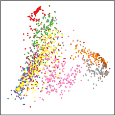
(a) v1

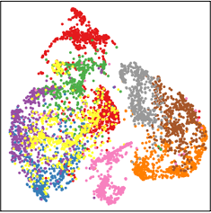
(b) v2

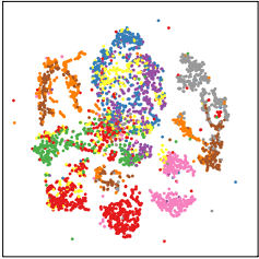
(c) Result of v1

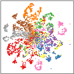
(d) Result of v2

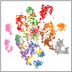
(e) Fused result

Figure 3: t-SNE visualization of original input and self-expressive matrices obtained by different strategy on the Fashion-MNIST dataset.

4.3 Expreimental Result

General Performance.

We perform the experiments on the four datasets, and report the results in Table 1. Our method consistently outperforms all other competitors. Particularly, when compared with gLMSC, our method outperforms it in terms of all the three metrics. This may be because that gLMSC aims to capture the comprehensive information among all views. However, not all the information in each view is helpful for discovering the subspace structures of the data. Thus, it is necessary to discard superfluous information while preserve useful information for boosting the performance of subspace clustering. Moreover, our method achieves better performance than MIB-DSC in terms of the three evaluation metrics on all the datasets. This demonstrates that utilizing the latent representation of one view as a self-supervised signal to guide the latent representation learning of other view is beneficial to subspace clustering. In addition, when compared with multi-view clustering methods, SiMVC and CoMVC, our method still obtains superior performance, illustrating that discovering the subspace structure of the data is important for clustering in many real-world applications.

Effect of Different Sizes of Data.

We test the performance of the subspace clustering methods using different sizes of data on the Fashion-MNIST dataset. The results are listed in Table 2. We can seet that our proposed method still outperforms other approaches when varying the sizes of the data. This further verifies the effectiveness of our method. Note that we do not perform gLMSC when the number of sample is 10,000, due to its huge memory requirement.

No. Points	1000			5000			10000
Metric	ACC	NMI	ARI	ACC	NMI	ARI	ACC	NMI	ARI
LRR	56.1	61.9	41.7	55.1	62.5	41.5	51.9	62.5	39.9
DSCN	53.6	59.4	40.6	56.3	55.8	37.2	58.5	62.6	44.7
DPSC	56.0	60.6	42.6	59.9	58.4	42.5	60.4	61.5	45.4
LMVSC	60.0	60.4	44.6	64.9	64.1	50.9	61.8	62.4	47.9
SiMVC	62.2	60.8	45.8	67.8	65.6	54.9	68.2	66.9	54.3
CoMVC	67.4	62.6	50.1	72.7	67.0	56.8	72.9	67.5	57.9
DMSC	60.2	57.1	44.5	58.3	59.4	43.6	56.4	60.1	42.0
MvDSCN	63.3	57.4	44.5	67.1	60.6	51.2	63.2	58.8	47.6
gLMSC	63.8	63.8	45.5	61.3	64.8	47.4	$-$	$-$	$-$
MIB-DSC	65.6	63.6	49.0	69.0	65.4	54.8	67.1	61.9	49.6
SIB-MSC	72.5	65.2	55.5	74.7	66.1	58.7	73.4	69.4	58.4

Table 2: Clustering results (%) on the Fashion-MNIST dataset with different sizes of data.

Ablation Study.

We conduct the ablation study on the all four datasets. Considering the overall objective $\mathcal{L}$ in (15), since the self-expressiveness loss $\mathcal{L}_{self}$ and the reconstruction loss $\mathcal{L}_{r}$ are necessary for subspace clustering, we perform the experiments by removing one of the rest loss terms each time. We first test whether the view-specific feature is useful for multi-view subspace clustering, and set $\alpha=0$. Then, we test the effectiveness of the loss term $\mathcal{L}_{c}$ which consists of three losses as shown in (3.1). The experimental results are reported in Table 3. Each component in our method is helpful for multi-view subspace clustering.

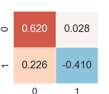
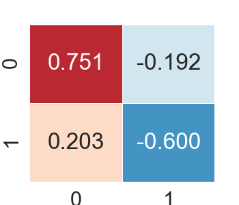
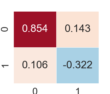
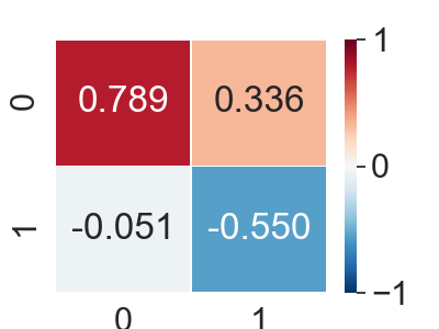
Figure 4: Correlations of different kinds of features. The left upper corner denotes the correlation between two view-common features $\mathbf{z}_{c}^{i}$ and $\mathbf{z}_{c}^{j}$. The right bottom corner denotes the correlation between two view-specific features $\mathbf{z}_{s}^{i}$ and $\mathbf{z}_{s}^{j}$. The left bottom measures the correlation between $\mathbf{z}_{s}^{j}$ and $\mathbf{z}_{c}^{j}$. The right upper corner is the correlation between $\mathbf{z}_{c}^{i}$ and $\mathbf{z}_{s}^{i}$.

Visualization.

To further understand the proposed model, we provide a visualization of the affinity matrix on the Fashion-MNIST dataset. The results are shown in Figure 3. Figure 3(c) and Figure 3(d) show the results of one of the two views respectively, while Figure 3(e) gives the result of the fused affinity matrix. We can clearly observe that the fused affinity matrix possesses better representation ability.

We also test the correlations between the view-common features and view-specific features using the cosine similarity on the Fashion-MNIST. We randomly select 4 samples and use their latent representations $\mathbf{z}$ to calculate the similarities. The results are shown in Figure 4. We can see that $\mathbf{z}_{c}^{i}$ and $\mathbf{z}_{c}^{j}$ have a relatively high correlation, while $\mathbf{z}_{c}^{i}$ and $\mathbf{z}_{s}^{i}$, $\mathbf{z}_{s}^{j}$ and $\mathbf{z}_{c}^{j}$ have relatively low correlations. This verifies the effectiveness of our proposed method.

	$\mathcal{L}_{s}$	$\mathcal{L}_{c}^{mkl}$	$\mathcal{L}_{c}^{cmi}$	$\mathcal{L}_{c}^{dis}$	ACC	NMI	ARI
RGBD	$-$	✓	✓	✓	43.8	66.5	24.5
	✓	$-$	✓	✓	41.8	65.3	22.7
	✓	✓	$-$	✓	29.2	55.2	11.6
	✓	✓	✓	$-$	48.1	69.3	28.9
	✓	✓	✓	✓	51.2	71.1	31.7
Fashion	$-$	✓	✓	✓	68.5	64.9	51.6
	✓	$-$	✓	✓	64.9	61.5	48.5
	✓	✓	$-$	✓	63.0	55.8	43.1
	✓	✓	✓	$-$	68.3	64.6	50.9
	✓	✓	✓	✓	72.5	65.2	55.5
notMNIST	$-$	✓	✓	✓	55.0	48.1	36.1
	✓	$-$	✓	✓	59.3	54.2	38.5
	✓	✓	$-$	✓	58.4	52.1	42.0
	✓	✓	✓	$-$	59.0	52.5	39.5
	✓	✓	✓	✓	61.9	55.8	42.7
COIL20	$-$	✓	✓	✓	77.8	82.1	70.3
	✓	$-$	✓	✓	73.2	82.2	69.2
	✓	✓	$-$	✓	51.4	64.5	39.2
	✓	✓	✓	$-$	68.8	75.7	59.7
	✓	✓	✓	✓	78.4	84.1	72.8

Table 3: Ablation study on all the four datasets.

5 Conclusion

In this paper, we proposed a new framework for multi-view deep subspace clustering from an information-theoretic point of view. We extended information bottleneck to learn the view-common information, where the latent representation of each view served as a self-supervised signal to capture the common information. Moreover, we attempted to capture the view-specific feature via mutual information to further boost the model performance. Experimental results on four publicly available datasets verified the effectiveness of our model.

References

- Abavisani and Patel [2018] Mahdi Abavisani and Vishal M Patel. Deep multimodal subspace clustering networks. J-STSP, 12(6):1601–1614, 2018.
- Alemi et al. [2017] Alexander A. Alemi, Ian Fischer, Joshua V. Dillon, and Kevin Murphy. Deep variational information bottleneck. In ICLR, 2017.
- Bulatov [2011] Yaroslav Bulatov. Notmnist dataset. Google (Books/OCR), Tech. Rep.[Online]. Available: http://yaroslavvb. blogspot. it/2011/09/notmnist-dataset. html, 2, 2011.
- Cao et al. [2015] Xiaochun Cao, Changqing Zhang, Huazhu Fu, Si Liu, and Hua Zhang. Diversity-induced multi-view subspace clustering. In CVPR, pages 586–594, 2015.
- Federici et al. [2020] Marco Federici, Anjan Dutta, Patrick Forré, Nate Kushman, and Zeynep Akata. Learning robust representations via multi-view information bottleneck. In ICLR, 2020.
- Gao et al. [2015] Hongchang Gao, Feiping Nie, Xuelong Li, and Heng Huang. Multi-view subspace clustering. In ICCV, pages 4238–4246, 2015.
- Gretton et al. [2005] Arthur Gretton, Olivier Bousquet, Alex Smola, and Bernhard Schölkopf. Measuring statistical dependence with hilbert-schmidt norms. In ALT, pages 63–77, 2005.
- Günnemann et al. [2012] Stephan Günnemann, Ines Färber, and Thomas Seidl. Multi-view clustering using mixture models in subspace projections. In KDD, pages 132–140, 2012.
- Ji et al. [2017] Pan Ji, Tong Zhang, Hongdong Li, Mathieu Salzmann, and Ian Reid. Deep subspace clustering networks. In NeurIPS, 2017.
- Kang et al. [2020] Zhao Kang, Wangtao Zhou, Zhitong Zhao, Junming Shao, Meng Han, and Zenglin Xu. Large-scale multi-view subspace clustering in linear time. In AAAI, pages 4412–4419, 2020.
- Lai et al. [2011] Kevin Lai, Liefeng Bo, Xiaofeng Ren, and Dieter Fox. A large-scale hierarchical multi-view rgb-d object dataset. In ICRA, pages 1817–1824, 2011.
- Li et al. [2021] Changsheng Li, Chen Yang, Bo Liu, Ye Yuan, and Guoren Wang. Lrsc: Learning representations for subspace clustering. In AAAI, pages 8340–8348, 2021.
- Liu et al. [2012] Guangcan Liu, Zhouchen Lin, Shuicheng Yan, Ju Sun, Yong Yu, and Yi Ma. Robust recovery of subspace structures by low-rank representation. TPAMI, 35(1):171–184, 2012.
- Motiian et al. [2016] Saeid Motiian, Marco Piccirilli, Donald A Adjeroh, and Gianfranco Doretto. Information bottleneck learning using privileged information for visual recognition. In CVPR, pages 1496–1505, 2016.
- Nene et al. [1996] Sameer A. Nene, Shree K. Nayar, and Hiroshi Murase. Columbia object image library (coil-20). Technical report, 1996.
- Ng et al. [2002] Andrew Y Ng, Michael I Jordan, and Yair Weiss. On spectral clustering: Analysis and an algorithm. In NeurIPS, pages 849–856, 2002.
- Nowozin et al. [2016] Sebastian Nowozin, Botond Cseke, and Ryota Tomioka. f-gan: Training generative neural samplers using variational divergence minimization. In NeurIPS, pages 271–279, 2016.
- Schmidhuber [1992] Jürgen Schmidhuber. Learning factorial codes by predictability minimization. Neural Computation, 4(6):863–879, 1992.
- Tishby et al. [2000] Naftali Tishby, Fernando C Pereira, and William Bialek. The information bottleneck method. arXiv preprint physics/0004057, 2000.
- Trosten et al. [2021] Daniel J Trosten, Sigurd Lokse, Robert Jenssen, and Michael Kampffmeyer. Reconsidering representation alignment for multi-view clustering. In CVPR, pages 1255–1265, 2021.
- Wan et al. [2021] Zhibin Wan, Changqing Zhang, Pengfei Zhu, and Qinghua Hu. Multi-view information-bottleneck representation learning. In AAAI, pages 10085–10092, 2021.
- Wu et al. [2020] Tailin Wu, Hongyu Ren, Pan Li, and Jure Leskovec. Graph information bottleneck. In NeurIPS, 2020.
- Xiao et al. [2017] Han Xiao, Kashif Rasul, and Roland Vollgraf. Fashion-mnist: a novel image dataset for benchmarking machine learning algorithms. arXiv preprint arXiv:1708.07747, 2017.
- Yu et al. [2021] Junchi Yu, Tingyang Xu, Yu Rong, Yatao Bian, Junzhou Huang, and Ran He. Graph information bottleneck for subgraph recognition. In ICLR, 2021.
- Zhang et al. [2015] Changqing Zhang, Huazhu Fu, Si Liu, Guangcan Liu, and Xiaochun Cao. Low-rank tensor constrained multiview subspace clustering. In ICCV, pages 1582–1590, 2015.
- Zhang et al. [2017] Changqing Zhang, Qinghua Hu, Huazhu Fu, Pengfei Zhu, and Xiaochun Cao. Latent multi-view subspace clustering. In CVPR, pages 4279–4287, 2017.
- Zhang et al. [2020] Changqing Zhang, Huazhu Fu, Qinghua Hu, Xiaochun Cao, Yuan Xie, Dacheng Tao, and Dong Xu. Generalized latent multi-view subspace clustering. TPAMI, 42(1):86–99, 2020.
- Zhou et al. [2019] Lei Zhou, Bai Xiao, Xianglong Liu, Jun Zhou, Edwin R Hancock, et al. Latent distribution preserving deep subspace clustering. In IJCAI, pages 4440–4446, 2019.
- Zhu et al. [2019] Pengfei Zhu, Binyuan Hui, Changqing Zhang, Dawei Du, Longyin Wen, and Qinghua Hu. Multi-view deep subspace clustering networks. arXiv preprint arXiv:1908.01978, 2019.