From Hyperbolic Geometry Back to Word Embeddings

Abstract

We choose random points in the hyperbolic disc and claim that these points are already word representations. However, it is yet to be uncovered which point corresponds to which word of the human language of interest. This correspondence can be approximately established using a pointwise mutual information between words and recent alignment techniques.

From Hyperbolic Geometry Back to Word Embeddings

Sultan Nurmukhamedov Yandex School of Data Analysis soltustik@gmail.com                        Thomas Mach University of Potsdam mach@uni-potsdam.de

Arsen Sheverdin University of Amsterdam arsen.sheverdin@student.uva.nl                        Zhenisbek Assylbekov Nazarbayev University zhassylbekov@nu.edu.kz

1 Introduction

Vector representations of words are ubiquitous in modern natural language processing (NLP). There are currently two large classes of word embedding models: they build (1) static and (2) contextualized word vectors correspondingly.

Static embeddings map each word type into a vector of real numbers, regardless of the context in which the word type is used. The most prominent representatives of this class of models are word2vec Mikolov et al. (2013b, a) and GloVe Pennington et al. (2014). The obvious problem with this approach is the representation of polysemous words, such as bank—it becomes unclear whether we are talking about a financial institution, or we are talking about the river bank.

Contextualized word embeddings, such as ELMo Peters et al. (2018) and BERT Devlin et al. (2019), solve this problem by mapping each word token into a vector space depending on the context in which the given word token is used, i.e. the same word will have different vector representations when used in different contexts. The second approach can nowadays be considered mainstream, despite relatively few papers offering theoretical justifications for contextualized word embeddings.

For static embeddings, on the contrary, there is a number of theoretical works, each of which offers its own version of what is happening when word vectors are trained. An incomplete list of such works includes those of Levy and Goldberg (2014), Arora et al. (2016), Hashimoto et al. (2016), Gittens et al. (2017), Tian et al. (2017), Ethayarajh et al. (2019), Allen et al. (2019), Allen and Hospedales (2019), Assylbekov and Takhanov (2019), Zobnin and Elistratova (2019). Other advantages of static embeddings over contextualized ones include faster training (few hours instead of few days) and lower computing requirements (1 consumer-level GPU instead of 8–16 non-consumer GPUs). Morevoer, static embeddings are still an integral part of deep neural network models that produce contextualized word vectors, because embedding lookup matrices are used at the input and output (softmax) layers of such models. Therefore, we consider it necessary to further study static embeddings.

Several recent works Nickel and Kiela (2017); Tifrea et al. (2019) argue that static word embeddings should be better trained in hyperbolic spaces than in Euclidean spaces, and provide empirical evidence that word embeddings trained in hyperbolic spaces need less dimensions to achieve the same quality as state-of-the-art Euclidean vectors. Usually such works motivate the hyperbolicity of word embeddings by the fact that hyperbolic spaces are better suited for embedding hierarchical structures. Words themselves often denote concepts with an underlying hierarchy. An example of such a hierarchy is the WordNet database, an excerpt of which is shown in Fig. 1.

Figure 1: An excerpt from the WordNet database.

In the present paper we will investigate where the hyperbolicity originates from. If we take the state-of-the-art Euclidean embeddings, is it possible to establish a direct connection between them and their counterparts from a hyperbolic word embedding? This was answered positively by Assylbekov and Jangeldin (2020) who established a chain of connections: from word embeddings to co-occurrence matrices, then to complex networks, and, finally, to hyperbolic spaces. In this paper, to provide an additional justification for the constructed chain, we propose a way to move from the final point, hyperbolic spaces, to the initial one, word embeddings. We show that drawing random points from the hyperbolic plane results in a set of points that reasonably well resembles word embeddings. In fact, we can match these points to word embeddings. Contrary, the same trick does not work with points drawn at random in the Euclidean space. Thus, one can argue that the hyperbolic space provides the underlying structure for word embeddings, while in the Euclidean space this structure has to be superimposed.

Notation

We denote with $\mathbb{R}$ the real numbers. Bold-faced lowercase letters ($\mathbf{x}$) denote vectors, plain-faced lowercase letters ($x$) denote scalars, bold-faced uppercase letters ($\mathbf{A}$) denote matrices, $\langle\mathbf{x},\mathbf{y}\rangle$ is the Euclidean inner product. We use $\mathbf{A}_{a:b,c:d}$ to denote a submatrix located at the intersection of rows $a,a+1,\ldots,b$ and columns $c,c+1,\ldots,d$ of $\mathbf{A}$. ‘i.i.d.’ stands for ‘independent and identically distributed’, ‘p.d.f’ stands for ‘probability distribution function’. We use the sign $\propto$ to abbreviate ‘proportional to’, and the sign $\sim$ to abbreviate ‘distributed as’.

Assuming that words have already been converted into indices, let $\mathcal{W}:=\{1,\ldots,n\}$ be a finite vocabulary of words. Following the setup of the widely used word2vec model Mikolov et al. (2013a, b), we use two vectors per each word $i$: (1) $\mathbf{w}_{i}\in\mathbb{R}^{d}$ when $i\in\mathcal{W}$ is a center word, (2) $\mathbf{c}_{i}\in\mathbb{R}^{d}$ when $i\in\mathcal{W}$ is a context word; and we assume that $d\ll n$.

In what follows we assume that our dataset consists of co-occurence pairs $(i,j)$. We say that “the words $i$ and $j$ co-occur” when they co-occur in a fixed-size window of words. Let $\#(i,j)$ be the number of times the words $i$ and $j$ co-occur.

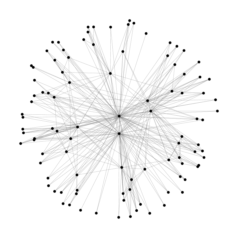
Figure 2: Random hyperbolic graph.

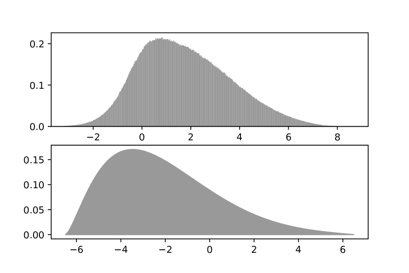
Figure 3: Distribution of PMI values (top) and of $R-X$.

2 Background: From Word Embeddings to Hyperbolic Space

Our departure point is the skip-gram with negative sampling (SGNS) word embedding model of Mikolov et al. (2013b) that maximizes the following objective function

$$\sum_{i\in\mathcal{W}}\sum_{j\in\mathcal{W}}\#(i,j)\log\sigma(\langle\mathbf{w}_{i},\mathbf{c}_{j}\rangle)\\ +k\cdot\mathbb{E}_{j^{\prime}\sim p}[\log\sigma(-\langle\mathbf{w}_{i},\mathbf{c}_{j^{\prime}}\rangle)],$$ (1)

where $\sigma(x)=\frac{1}{1+e^{-x}}$ is the logistic sigmoid function, $p$ is a smoothed unigram probability distribution for words, and $k$ is the number of negative samples to be drawn. Interestingly, training SGNS is approximately equivalent to finding a low-rank approximation of a shifted pointwise mutual information (PMI) matrix Levy and Goldberg (2014) in the form

$$\log\frac{p(i,j)}{p(i)p(j)}-\log k\approx\langle\mathbf{w}_{i},\mathbf{c}_{j}\rangle,$$ (2)

where the left-hand side is the shifted PMI between $i$ and $j$, and the right-hand side is an $ij$-th element of a matrix with rank $\leq d$ since $\mathbf{w}_{i},\mathbf{c}_{j}\in\mathbb{R}^{d}$. This approximation was later re-derived by Arora et al. (2016), Zobnin and Elistratova (2019), Assylbekov and Takhanov (2019), and Allen et al. (2019) under different sets of assuptions. In a recent paper, Assylbekov and Jangeldin (2020) showed that the removal of the sigmoid transformation in the SGNS objective (1) gives word embeddings comparable in quality with the original SGNS embeddings. A maximization of such modified objective results in a low-rank approximation of a squashed shifted PMI ($\sigma$SPMI) matrix, defined as

$$\mathbf{A}_{ij}:=\sigma\left(\log\frac{p(i,j)}{p(i)p(j)}-\log k\right).$$ (3)

Moreover, treating the $\sigma$SPMI matrix as a connection probabilities matrix of a random graph, the authors show that such graph is a complex network, that is it has strong clustering and scale-free degree distribution, and according to Krioukov et al. (2010), such graph possesses an effective hyperbolic geometry underneath. The following chain summarizes this argument:

$$\boxed{\text{Word Embeddings}}\quad\longrightarrow\quad\boxed{\sigma\text{SPMI}}\quad\longrightarrow\\ \boxed{\text{Complex Network}}\quad\longrightarrow\quad\boxed{\text{Hyperbolic Space}}$$ (4)

In our work, we go from the final point (hyperbolic space) to the starting one (word embeddings), and the next section provides the details of our method.

Method	Word Similarity			POS Tagging
	WS353	Men	M. Turk	CoNLL-2000	Brown
SGNS	.678	.656	.690	90.77	92.60
PMI + SVD	.669	.674	.666	92.25	93.76
$\sigma$SPMI + SVD	.648	.622	.666	92.76	93.78
RHG + SVD + Align	.406	.399	.509	92.23	93.19
Random + Align	.165	.117	.111	81.89	89.39

Table 1: Evaluation of word embeddings on the similarity and POS tagging tasks. For the similarity tasks the evaluation metric is the Spearman’s correlation with human ratings, for the POS tagging tasks it is accuracy. Random stands for random vectors that were obtained as i.i.d. draws from $\mathcal{N}(\mathbf{0},\mathbf{I})$.

3 Method: From Hyperbolic Geometry to Word Embeddings

It is difficult to visualize hyperbolic spaces because they cannot be isometrically embedded into any Euclidean space. However, there exist models of hyperbolic spaces: each model emphasizes different aspects of hyperbolic geometry, but no model simultaneously represents all of its properties. We will consider here the so-called native model Krioukov et al. (2010), in which the hyperbolic plane $\mathbb{H}^{2}$ is represented by a disk of radius $R$, and we use polar coordinates $(r,\theta)$ to specify the position of any point $v\in\mathbb{H}^{2}$, where the radial coordinate $r$ equals the hyperbolic distance of $v$ from the origin. Given this notation, the distance $x$ between two points with coordinates $(r,\theta)$ and $(r^{\prime},\theta^{\prime})$ satisfies the hyperbolic law of cosines

$$\textstyle\cosh x=\cosh r\cosh r^{\prime}\\ -\sinh r\sinh r^{\prime}\cos(\theta-\theta^{\prime}),$$ (5)

for the hyperbolic space of constant curvature $-1$. A key property of hyperbolic spaces is that they expand faster than Euclidean spaces. E.g., a circle with radius $r$ has in the Euclidean plane a length of $2\pi r=\Theta(r)$ and an area of $\pi r^{2}=\Theta(r^{2})$, while its length and area in the hyperbolic plane are $2\pi\sinh(r)=\Theta(e^{r})$ and $2\pi(\cosh r-1)=\Theta(e^{r})$ correspondingly. It is noteworthy that in a balanced tree with branching factor $b$, the number of nodes that are $r$ edges from the root grows as $\Theta(b^{r})$, i.e. exponentially with $r$, leading to the suggestion that hierarchical complex networks with tree-like structures might be easily embeddable in hyperbolic space.

Based on the above facts, we construct a random hyperbolic (RHG) graph as in the work of Krioukov et al. (2010): we place randomly $n$ points (nodes) into a hyperbolic disk of radius $R$, and each pair of nodes $(i,j)$ is connected with probability $\sigma(R-x_{ij})$, where $x_{ij}$ is the hyperbolic distance (5) between points $i$ and $j$. Angular coordinates of the nodes are sampled from the uniform distribution: $\theta\sim\mathcal{U}[0,2\pi]$, while the radial coordinates are sampled from the exponential p.d.f.

$$\rho(r)=\frac{\alpha\sinh\alpha r}{\cosh\alpha R-1}=\Theta(e^{\alpha r}).$$

The hyperparameters $R$ and $\alpha$ are chosen based on the total number of nodes $n$, the desired average degree $\bar{k}$ and the power-law exponent $\gamma$ according to the equations (22) and (29) of Krioukov et al. (2010). An example of such RHG is shown in Figure 3. Notice, that the connection probabilities matrix of our graph is

$$\mathbf{B}_{ij}:=\sigma(R-x_{ij}),$$

Comparing this to (3), we see that if $\mathbf{A}$ and $\mathbf{B}$ induce structurally similar graphs then the distribution of the PMI values $\log\frac{p(i,j)}{p(i)p(j)}$ should be similar to the distribution of $R-x_{ij}$ values (up to a constant shift). To test this empirically, we compute a PMI matrix of a well-known corpus, text8, and compare the distribution of the PMI values with the p.d.f. of $R-X$, where $X$ is a distance between two random points of a hyperbolic disk (the exact form of this p.d.f. is given in Proposition A.1). The results are shown in Figure 3. As we can see, the two distributions are similar in the sense that both are unimodal and right-skewed. The main difference is in the shift—distribution of $R-X$ is shifted to the left compared to the distribution of the PMI values.

We hypothesize that the nodes of the RHG treated as points of the hyperbolic space are already reasonable word embeddings for the words of our vocabulary $\mathcal{W}$. The only thing that we do not know is the correspondence between words $i\in\mathcal{W}$ and nodes of the RHG. Instead of aligning words with nodes, we can align their vector representations. For this, we take singular value decompositions (SVD) of $\mathbf{A}$ and $\mathbf{B}$:

$$\mathbf{A}=\mathbf{U}_{A}\boldsymbol{\Sigma}_{A}\mathbf{V}_{A}^{\top},\quad\mathbf{B}=\mathbf{U}_{B}\boldsymbol{\Sigma}_{B}\mathbf{V}_{B}^{\top},$$

and then obtain embedding matrices by

$$\mathbf{W}_{A} :=\mathbf{U}_{A,1:n,1:d}\boldsymbol{\Sigma}^{1/2}_{A,1:d,1:d}\in\mathbb{R}^{n\times d}$$

$$\mathbf{W}_{B} :=\mathbf{U}_{B,1:n,1:d}\boldsymbol{\Sigma}^{1/2}_{B,1:d,1:d}\in\mathbb{R}^{n\times d}$$

as in the work of Levy and Goldberg (2014). An $i^{\text{th}}$ row in $\mathbf{W}_{A}$ is an embedding of the word $i\in\mathcal{W}$, while an $i^{\text{th}}$ row in $\mathbf{W}_{B}$ is an embedding of the RHG’s node $i$. To align these two sets of embeddings we apply a recent stochastic optimization method of Grave et al. (2019) that solves

$$\min_{\mathbf{Q}\in\mathcal{O}_{d}}\min_{\mathbf{P}\in\mathcal{P}_{n}}\|\mathbf{W}_{A}\mathbf{Q}-\mathbf{P}\mathbf{W}_{B}\|^{2}_{2},$$

where $\mathcal{O}_{d}$ is the set of $d\times d$ orthogonal matrices and $\mathcal{P}_{d}$ is the set of $n\times n$ permutation matrices. As one can see, this method assumes that alignment between two sets of embeddings is not only a permutation from one set to the other, but also an orthogonal transformation between the two. Once the alignment is done, we treat $\mathbf{PW}_{B}$ as an embedding matrix for the words in $\mathcal{W}$.

4 Evaluation

In this section we evaluate the quality of word vectors resulting from a RHG against those from the SGNS, PMI, and $\sigma$SPMI. We use the text8 corpus mentioned in the previous section. We were ignoring words that appeared less than 5 times (resulting in a vocabulary of 71,290 tokens). We set window size to 2, subsampling threshold to $10^{-5}$, and dimensionality of word vectors to 200. The SGNS embeddings were trained using our custom implementation. The PMI and BPMI matrices were extracted using the hyperwords tool of Levy et al. (2015) and SVD was performed using the PyTorch library of Paszke et al. (2019).

The embeddings were evaluated on word similarity and POS tagging tasks. For word similarity we used WordSim (Finkelstein et al., 2002), MEN (Bruni et al., 2012), and M.Turk (Radinsky et al., 2011) datasets. For POS tagging we trained a simple classifier by feeding in the embedding of a current word and its nearby context to predict its part-of-speech (POS) tag:

$$\widehat{\mathrm{POS}}_{t}=\operatorname{softmax}(\sigma(\mathbf{A}[\mathbf{w}_{t-2};\ldots;\mathbf{w}_{t+2}]+\mathbf{b}))$$

where $[\mathbf{x};\mathbf{y}]$ is concatenation of $\mathbf{x}$ and $\mathbf{y}$. The classifier was trained on CoNLL-2000 Tjong Kim Sang and Buchholz (2000) and Brown Kucera et al. (1967) datasets.

The results of evaluation are provided in Table 1. As we see, vector representations of words generated from a RHG lag behind in word similarity tasks from word vectors obtained by other standard methods. Note, however, that the similarity task was designed with Euclidean geometry in mind. Even though our RHG-based vectors are also ultimately placed in the Euclidean space (otherwise the alignment step would not have been possible), their nature is inherently non-Euclidean. Therefore, the similarity scores for them may not be indicative. So, for example, when RHG vectors are fed into a nonlinear model for POS tagging, they are comparable with other types of vectors.

We notice that random vectors—generated as i.i.d. draws from $\mathcal{N}(\mathbf{0},\mathbf{I})$ and then aligned to the embeddings from $\sigma$SPMI—show poor results in the similarity tasks and underperform all other word embedding methods in the POS tagging tasks. This calls into question whether multivariate Gaussian is a reasonable (prior) distribution for word vectors as was suggested by Arora et al. (2016), Assylbekov and Takhanov (2019).

5 Conclusion and Future Work

In this work we show that word vectors can be obtained from hyperbolic geometry without explicit training. We obtain the embeddings by randomly drawing points in the hyperbolic plane and by finding correspondence between these points and the words of the human language. This correspondence is determined by the relation (hyperbolic distance) to other words. This method avoids the, often expensive, training of word vectors in hyperbolic spaces as in Tifrea et al. (2019). A direct comparison is not what this paper attempts—our method is cheaper but produces word vectors of lower quality. Our method simply shows that word vectors do fit better into hyperbolic space than into Euclidean space.

Finally, we want to sketch a possible direction for future work. The hyperbolic space is a special case of a Riemannian manifold. Are Riemannian manifolds better suited for word vectors? In particular which manifolds should one use? At the moment, there is only limited empirical knowledge to address these questions. For instance, Gu et al. (2019) obtained word vectors of better quality, according to the similarity score, in the product of hyperbolic spaces, which is still a Riemannian manifold but not a hyperbolic space anymore. We are hopeful that future work may provide an explanation for this empirical fact.

Appendix A Auxiliary Results

Proposition A.1.

Let $X$ be a distance between two points that were randomly uniformly placed in the hyperbolic disk of radius $R$. The probability distribution function of $X$ is given by

$$f_{X}(x)=\int_{0}^{R}\int_{0}^{R}\\ \frac{\sinh(x)\rho(r_{1})\rho(r_{2})dr_{1}dr_{2}}{\pi\sqrt{1-A(r_{1},r_{2},x)}\sinh(r_{1})\sinh(r_{2})},$$ (6)

where $A(r_{1},r_{2},x)=\frac{\cosh(r_{1})\cosh(r_{2})-\cosh(x)}{\sinh(r_{1})\sinh(r_{2})}$, and $\rho(r)=\frac{\alpha\sinh\alpha r}{\cosh\alpha R-1}$.

Proof.

Let us throw randomly and uniformly two points $(r_{1},\theta_{1})$ and $(r_{2},\theta_{2})$ into the hyperbolic disk of radius $R$, i.e. $r_{1},r_{2}\,\,{\stackrel{{\scriptstyle\text{i.i.d.}}}{{\sim}}}\,\,\rho(r)$, $\theta_{1},\theta_{2}\,\,{\stackrel{{\scriptstyle\text{i.i.d.}}}{{\sim}}}\,\,\text{Uniform}[0,2\pi)$. Let $X$ be the distance between these points ($X$ is a random variable). Let $\gamma$ be the angle between these points, then $\gamma:=\pi-|\pi-|\theta_{1}-\theta_{2}||\sim\text{Uniform}[0,\pi)$ and thus

$$f_{\cos\gamma}(t)=\frac{1}{\pi\sqrt{1-t^{2}}},\quad t\in[-1,1].$$

Since the distance in our model of hyperbolic plane is given by

$$X=\cosh^{-1}[\cosh r_{1}\cosh r_{2}-\sinh r_{1}\sinh r_{2}\cos\gamma]$$

we have

$$\Pr(X\leq x)$$

$$=\Pr\left(\cos\gamma\geq\underbrace{\frac{\cosh r_{1}\cosh r_{2}-\cosh x}{\sinh r_{1}\sinh r_{2}}}_{A(r_{1},r_{2},x)}\right)$$

$$=\Pr(\cos\gamma\geq A(r_{1},r_{2},x))$$

$$=\int_{A(r_{1},r_{2},x)}^{+\infty}\frac{1}{\pi\sqrt{1-t^{2}}}$$

$$=\frac{1}{2}-\frac{\sin^{-1}A(r_{1},r_{2},x)}{\pi},$$

and therefore

$$f_{X\mid r_{1},r_{2}}(x)=\frac{d}{dx}\left[\frac{1}{2}-\frac{\sin^{-1}A(r_{1},r_{2},x)}{\pi}\right]\\ =\frac{\sinh x}{\pi\sqrt{1-A(r_{1},r_{2},x)}\sinh(r_{1})\sinh r_{2}}$$

for $x\in(|r_{1}-r_{2}|,r_{1}+r_{2})$. Integrating $f_{X\mid r_{1},r_{2}}(x)\rho(r_{1})\rho(r_{2})$ with respect to $r_{1}$ and $r_{2}$ we get (6). ∎

References

- Allen et al. (2019) Carl Allen, Ivana Balazevic, and Timothy Hospedales. 2019. What the vec? towards probabilistically grounded embeddings. In Proceedings of NeurIPS.
- Allen and Hospedales (2019) Carl Allen and Timothy Hospedales. 2019. Analogies explained: Towards understanding word embeddings. In Proceedings of ICML.
- Arora et al. (2016) Sanjeev Arora, Yuanzhi Li, Yingyu Liang, Tengyu Ma, and Andrej Risteski. 2016. A latent variable model approach to pmi-based word embeddings. Transactions of the Association for Computational Linguistics, 4:385–399.
- Assylbekov and Jangeldin (2020) Zhenisbek Assylbekov and Alibi Jangeldin. 2020. Squashed shifted pmi matrix: bridging word embeddings and hyperbolic spaces. In Proceedings of AJCAI.
- Assylbekov and Takhanov (2019) Zhenisbek Assylbekov and Rustem Takhanov. 2019. Context vectors are reflections of word vectors in half the dimensions. Journal of Artificial Intelligence Research, 66:225–242.
- Bruni et al. (2012) Elia Bruni, Gemma Boleda, Marco Baroni, and Nam-Khanh Tran. 2012. Distributional semantics in technicolor. In Proceedings of ACL.
- Devlin et al. (2019) Jacob Devlin, Ming-Wei Chang, Kenton Lee, and Kristina Toutanova. 2019. Bert: Pre-training of deep bidirectional transformers for language understanding. In Proceedings of NAACL-HLT.
- Ethayarajh et al. (2019) Kawin Ethayarajh, David Duvenaud, and Graeme Hirst. 2019. Towards understanding linear word analogies. In Proceedings of ACL.
- Finkelstein et al. (2002) Lev Finkelstein, Evgeniy Gabrilovich, Yossi Matias, Ehud Rivlin, Zach Solan, Gadi Wolfman, and Eytan Ruppin. 2002. Placing search in context: The concept revisited. ACM Transactions on information systems, 20(1):116–131.
- Gittens et al. (2017) Alex Gittens, Dimitris Achlioptas, and Michael W Mahoney. 2017. Skip-gram- zipf+ uniform= vector additivity. In Proceedings of ACL, pages 69–76.
- Grave et al. (2019) Edouard Grave, Armand Joulin, and Quentin Berthet. 2019. Unsupervised alignment of embeddings with wasserstein procrustes. In Proceedings of AISTATS.
- Gu et al. (2019) Albert Gu, Frederic Sala, Beliz Gunel, and Christopher Ré. 2019. Learning mixed-curvature representations in product spaces. In 7th International Conference on Learning Representations, ICLR 2019, New Orleans, LA, USA, May 6-9, 2019. OpenReview.net.
- Hashimoto et al. (2016) Tatsunori B Hashimoto, David Alvarez-Melis, and Tommi S Jaakkola. 2016. Word embeddings as metric recovery in semantic spaces. Transactions of the Association for Computational Linguistics, 4:273–286.
- Krioukov et al. (2010) Dmitri Krioukov, Fragkiskos Papadopoulos, Maksim Kitsak, Amin Vahdat, and Marián Boguná. 2010. Hyperbolic geometry of complex networks. Physical Review E, 82(3):036106.
- Kucera et al. (1967) Henry Kucera, Henry Kučera, and Winthrop Nelson Francis. 1967. Computational analysis of present-day American English. Brown university press.
- Levy and Goldberg (2014) Omer Levy and Yoav Goldberg. 2014. Neural word embedding as implicit matrix factorization. In Proceedings of NeurIPS.
- Levy et al. (2015) Omer Levy, Yoav Goldberg, and Ido Dagan. 2015. Improving distributional similarity with lessons learned from word embeddings. Transactions of the Association for Computational Linguistics, 3:211–225.
- Mikolov et al. (2013a) Tomas Mikolov, Kai Chen, Greg Corrado, and Jeffrey Dean. 2013a. Efficient estimation of word representations in vector space. arXiv preprint arXiv:1301.3781.
- Mikolov et al. (2013b) Tomas Mikolov, Ilya Sutskever, Kai Chen, Greg S Corrado, and Jeff Dean. 2013b. Distributed representations of words and phrases and their compositionality. In Proceedings of NeurIPS.
- Nickel and Kiela (2017) Maximillian Nickel and Douwe Kiela. 2017. Poincaré embeddings for learning hierarchical representations. In Advances in neural information processing systems, pages 6338–6347.
- Paszke et al. (2019) Adam Paszke, Sam Gross, Francisco Massa, Adam Lerer, James Bradbury, Gregory Chanan, Trevor Killeen, Zeming Lin, Natalia Gimelshein, Luca Antiga, et al. 2019. Pytorch: An imperative style, high-performance deep learning library. In Proceedings of NeurIPS.
- Pennington et al. (2014) Jeffrey Pennington, Richard Socher, and Christopher Manning. 2014. Glove: Global vectors for word representation. In Proceedings of EMNLP.
- Peters et al. (2018) Matthew E Peters, Mark Neumann, Mohit Iyyer, Matt Gardner, Christopher Clark, Kenton Lee, and Luke Zettlemoyer. 2018. Deep contextualized word representations. In Proceedings of NAACL-HLT.
- Radinsky et al. (2011) Kira Radinsky, Eugene Agichtein, Evgeniy Gabrilovich, and Shaul Markovitch. 2011. A word at a time: computing word relatedness using temporal semantic analysis. In Proceedings of the 20th international conference on World wide web, pages 337–346. ACM.
- Tian et al. (2017) Ran Tian, Naoaki Okazaki, and Kentaro Inui. 2017. The mechanism of additive composition. Machine Learning, 106(7):1083–1130.
- Tifrea et al. (2019) Alexandru Tifrea, Gary Bécigneul, and Octavian-Eugen Ganea. 2019. Poincaré glove: Hyperbolic word embeddings. In Proceedings of ICLR.
- Tjong Kim Sang and Buchholz (2000) Erik F. Tjong Kim Sang and Sabine Buchholz. 2000. Introduction to the CoNLL-2000 shared task chunking. In Fourth Conference on Computational Natural Language Learning and the Second Learning Language in Logic Workshop.
- Zobnin and Elistratova (2019) Alexey Zobnin and Evgenia Elistratova. 2019. Learning word embeddings without context vectors. In Proceedings of the 4th Workshop on Representation Learning for NLP (RepL4NLP-2019), pages 244–249.