A thinning-based representation of the compound-Poisson INGARCH model, with an interpretation as a stochastic epidemic process

Abstract

A thinning-based representation of the Poisson and certain compound Poisson (CP) INGARCH models is proposed. This approaches them to the INAR model class, which is equally thinning-based, and allows for the application of branching process theory to derive stochastic properties. Notably, it is straightforward to show that under mild conditions the CP-INGARCH(1, 1) model is geometrically ergodic while all moments of the limiting-stationary distribution are finite. Moreover, the new representation provides an interpretation of INGARCH models as a stochastic epidemic process, specifically a simplified discrete-time SEIR (susceptible-exposed-infectious-removed) model.

This is a preprint and has not been subject to peer-review.

1 Count autoregression based on thinnings and generalized linear regression

Two of the most influential approaches for count time series modelling are the INAR (interger-valued autoregressive) and INGARCH (integer-valued generalized autoregressive conditional heteroscedasticity) classes. The INAR class is built on the idea of thinning operations [27], most commonly the binomial thinning operator $\circ$, which is given by

$$\pi\circ N=\sum_{i=1}^{N}Z_{i}\ \ \ \text{with}\ \ \ Z_{i}\stackrel{{\scriptstyle\text{ind}}}{{\sim}}\text{Bin}(1,\pi).$$

The basic Poisson INAR(1) model $\{X_{t},t\in\mathbb{Z}\}$ [19, 1] is defined as

$$X_{t}=I_{t}+\kappa\circ X_{t-1},$$

where $0\leq\kappa\leq 1$ and $\{I_{t}\}$ is a sequence of independent Poisson random variables with rate $\nu=0$. This model has been extended in a multitude of ways [25]. The INGARCH class [10, 12], on the other hand, adopts the idea of generalized linear regression models (GLMs). Its simplest instance, the Poisson INARCH(1) model, is defined as a process $\{X_{t},t\in\mathbb{N}_{0}\}$ with

$$X_{t}\mid X_{t-1},\dots,X_{0} \sim\text{Pois}(\lambda_{t})$$

$$\lambda_{t} =\nu+\alpha X_{t-1},$$

$\nu>0,\alpha\geq 0$, and a fixed starting value $X_{0}$. The GLM-based perspective, too, has spawned extensive research [11]. It has been noted that the INARCH(1) model can also be written as [30]

$$X_{t}=I_{t}+\kappa\star X_{t-1}$$

with $I_{t}\stackrel{{\scriptstyle\text{ind}}}{{\sim}}\text{Pois}(\nu)$ as in the INAR(1) model and $\star$ denoting Poisson thinning,

$$\pi\star N=\sum_{i=1}^{N}Z_{i}\ \ \ \text{with}\ \ \ Z_{i}\stackrel{{\scriptstyle\text{ind}}}{{\sim}}\text{Pois}(\pi).$$

Occasionally, also more complex INGARCH models have been represented via thinning operations, see e.g. [18]. Indeed, the original construction of the INGARCH(1, 1) model involved a “cascade of thinning operations” [10, p.927]. By and large, however, the two classes have been treated separately. This note introduces a new thinning-based representation of several INGARCH models, thus providing a bridge to the INAR class. Also, the new representation allows for an intuitive interpretation as a stochastic epidemic process, similar to the so-called SEIR (susceptible-exposed-infectious-recovered) model from epidemiology. We start by stating the definitions of various INGARCH models, then provide their thinning-based representations and conclude by exploiting the novel formulation to obtain some stochastic properties.

2 Poisson and compound Poisson INGARCH models

The most common extension of the Poisson INARCH(1) model is the Poisson INGARCH(1, 1) model [10, 12]. It is defined as a process $\{X_{t},t\in\mathbb{N}_{0}\}$ with

$$X_{t}\mid X_{t-1},\dots,X_{0},\lambda_{0} \sim\text{Pois}(\lambda_{t})$$ (1)

$$\lambda_{t} =\nu+\alpha X_{t-1}+\beta\lambda_{t-1}$$ (2)

where $\nu>0,\alpha>0$ and $0\leq\beta<1$. Note that this is somewhat more restrictive than most definitions from the literature where $\alpha=0$ and $\beta\geq 1$ are usually allowed. The initial values $\lambda_{0}\geq\nu$ and $X_{0}\in\mathbb{N}_{0}$ are assumed to be fixed as in [12] (note that other authors, like [10], use index set $t\in\mathbb{Z}$ and thus do not require an initialization). More generally, to define the Poisson INGARCH($p$, $q$) model, equation (2) is replaced by

$$\lambda_{t}=\nu+\sum_{i=1}^{p}\alpha_{i}X_{t-i}+\sum_{j=1}^{q}\beta_{j}\lambda_{t-j},$$ (3)

and additional initial values $\lambda_{1-q},\dots,\lambda_{0}\geq\nu$ and $X_{1-p},\dots,X_{0}\in\mathbb{N}_{0}$ are fixed. We assume $\alpha_{i}>0,i=1,\dots,p$ and $\beta_{j}\geq 0,j=1,\dots,q$ with $\sum_{j=1}^{q}\beta_{j}<1$.

Numerous variations of model (1)–(2) with conditional distributions other than the Poisson have been suggested (see [28] for an overview). A broad class are compound Poisson INGARCH models [13, 26]. A random variable $Y$ is said to follow a compound Poisson distribution [9, Chapter 3] if it can be written as a randomly stopped sum

$$Y=\sum_{i=1}^{N}Z_{i},\ \ \ Z_{1},\dots,Z_{N}\stackrel{{\scriptstyle\text{iid}}}{{\sim}}G(\psi)$$

where $N$ follows a Poisson distribution. Throughout this article we assume that $G(\psi)$, also called the secondary distribution, is parameterized by a single parameter $\psi$ and has support $\mathbb{N}_{0}$. Its mean $\mu_{\psi}$ and variance $\sigma^{2}_{\psi}$ are assumed to be finite. Adapting notation from Weiß et al [31, Sec. 2], the CP-INGARCH(1, 1) model is defined as a process $\{X_{t},t\in\mathbb{N}_{0}\}$ with

$$N_{t}\ \mid\ X_{t-1},\dots,X_{0},\lambda_{0} \sim\text{Pois}(\lambda_{t}/\mu_{\psi})$$ (4)

$$X_{t} =\sum_{i=1}^{N_{t}}Z_{i,t}\ \ \text{where}\ \ Z_{i,t}\stackrel{{\scriptstyle\text{iid}}}{{\sim}}G(\psi)$$ (5)

$$\lambda_{t} =\nu+\alpha X_{t-1}+\beta\lambda_{t-1}.$$ (6)

Here, $\lambda_{0}\geq\nu$ and $X_{0}\in\mathbb{N}_{0}$ are again fixed. Conditional on the past, $X_{t}$ follows a compound Poisson distribution with mean $\lambda_{t}$ under this definition. This formulation is somewhat more restrictive than the class discussed in [13] where the parameter $\psi_{t}$ of the secondary distribution can depend on $\lambda_{t}$. It nonetheless contains a number of well-known models [13, Observation 2]:

• Setting $G(\psi)$ to a logarithmic distribution leads to a negative biomial INGARCH(1, 1) model ([32]; Example 4.2.1 in [28]).

• The Neyman Type A INGARCH model [14] results when setting $G(\psi)$ to a Poisson distribution.

• The generalized Poisson INGARCH(1, 1) model [33] is obtained by setting $G(\psi)$ to a Borel distribution.

3 Thinning-based representation of INGARCH models

3.1 The Poisson INGARCH(1, 1) model

We first provide an alternative representation of the Poisson INGARCH(1, 1) model (1)–(2). It involves exclusively discrete-valued random variables and is given by

$$X_{t} =I_{t}+E_{t}-L_{t}$$ (7)

$$E_{t} =L_{t-1}\ +\ \kappa\star X_{t-1}$$ (8)

$$L_{t} =\beta\circ E_{t}$$ (9)

where $\kappa>0$ and $0\leq\beta<1$. Here, $\{I_{t}\}$ consists of independent Poisson random variables with rate $\tau>0$ while $\circ$ and $\star$ denote binomial and Poisson thinning as defined in Section 1. To initialize the process we fix $X_{0}\in\mathbb{N}_{0},\eta>0$ and specify $E_{0}\sim\text{Pois}\left(\eta\right)$.

It can be shown that $\{X_{t}\}$ as defined in equation (7)–(9) is a Poisson INGARCH(1, 1) process as given in (1)–(2), see Appendix A.1 for the derivation. The parameter $\beta$ is shared across the two formulations, meaning that the INARCH(1) model corresponds to $\beta=0$. The remaining parameters of the original formulation can be recovered as $\nu=(1-\beta)\tau$ and $\ \ \alpha=(1-\beta)\kappa.$ Concerning the initialization, equivalence is achieved by setting $\lambda_{0}=\tau+(1-\beta)\times\eta$.

To facilitate verbal description and generalizations in the following sections, we introduce two auxiliary processes,

$$A_{t} =E_{t}-L_{t}$$ (10)

$$C_{t} =\kappa\star X_{t},$$ (11)

which allow us to re-write equations (7) and (8) as

$$X_{t} =I_{t}+A_{t}$$ (12)

$$E_{t} =L_{t-1}+C_{t-1}.$$ (13)

The Poisson INGARCH(1, 1) process (9)–(13) can be interpreted as a simple model for the spread of an infectious disease. A visualization is provided in Figure 1.

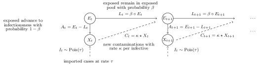
Figure 1: Interpretation of the Poisson INGARCH(1, 1) formulation (9)–(13) as a stochastic epidemic process. Solid lines represent results of binomial thinning, dashed lines Poisson thinning or immigration. Note that the two solid arrows starting at $E_{t}$ do not represent independent binomial thinnings as by construction $L_{t}+A_{t}=E_{t}$.

1. $X_{t}$ is the number of individuals who are infectious with a given disease at time $t$. Each of these individuals stays infectious for one time period and contaminates a $\text{Pois}(\kappa)$-distributed number $C_{t}=\kappa\star X_{t}$ of other individuals, exposing them to the disease.

2. Contaminated individuals enter into an exposed pool at the following time point $t+1$ (exposed meaning that they have contracted the disease, but are not infectious yet). The total number of exposed individuals present in the population at time $t+1$ is denoted by $E_{t+1}$.

3. At each time $t$, each of the $E_{t}$ exposed individuals can either remain in the exposed pool (with probability $\beta$) or advance to infectiousness, thus being removed from the pool (with probability $1-\beta$). The exposed individuals left from time $t$ are denoted by $L_{t}=\beta\circ E_{t}$ and form part of $E_{t+1}$. This construction implies that the latent period (time from contamination to infectiousness) is $\text{Geom}(1-\beta)$ distributed (see equation (27)).

4. If an exposed individual from $E_{t}$ advances to the infectious stage, it enters into $X_{t}$. The number of such individuals is denoted by $A_{t}=E_{t}-L_{t}$.

5. At each time $t$, a $\text{Pois}(\tau)$ distributed number $I_{t}$ of individuals become infectious due to external sources (imports).

This is similar to the mechanism of the so-called SEIR (susceptible-exposed-infectious-removed) model commonly used in epidemiology (see e.g. [5] for a textbook introduction). The INGARCH mechanism is simpler in that it models only the exposed and infectious groups explicitly, but not the susceptible and recovered/immunized. Consequently, it also ignores that any real population would be finite in size. The model will thus not capture the non-linear effects arising in the SEIR model due to the depletion of the susceptible population. For rare diseases in a large population or diseases with short-lived immunity (which can be described by an SEIS model, susceptible-exposed-infectious-susceptible), it may nonetheless be a reasonable approximation; see [3] for a related argument linking the SIR (susceptible-infectious-removed) and the INARCH(1) model.

Note that a related model where the Poisson thinning in equations (8)/(11) is replaced by a binomial thinning has been introduced in [4].

3.2 The Poisson INGARCH($p$, $q$) model

An extension of the thinning-based representation (9)–(13) to the INGARCH($p$, $q$) case is given by

$$X_{t} =I_{t}+A_{t}$$ (14)

$$E_{t} =\sum_{j=1}^{q}L_{t-j,j}\ \ +\ \ \sum_{i=1}^{p}C_{t-i,i}$$ (15)

where

$$C_{t,i} =\kappa_{i}\star X_{t}$$ (16)

$$(L_{t,1},\dots,L_{t,q},A_{t})\ \mid\ E_{t} \sim\text{Mult}\left(E_{t};\beta_{1},\dots,\beta_{q},1-\sum_{j=1}^{q}\beta_{j}\right)$$ (17)

and $\kappa_{i},\beta_{j}>0,\sum_{j=1}^{q}\beta_{j}<1$. For the initialization we fix $X_{1-p},\dots,X_{0}$ and set $E_{m}\sim\text{Pois}(\eta_{m})$ with $\eta_{m}>0$ for $m=1-q,\dots,0$. Again, the parameters $\beta_{1},\dots,\beta_{q}$ are the same as in the original formulation (3). The remaining parameters can be obtained as $\nu=\left(1-\sum_{j=1}^{q}\beta_{j}\right)\times\tau$ and $\alpha_{i}=\left(1-\sum_{j=1}^{q}\beta_{j}\right)\times\kappa_{i}$. For the initialization, one needs to set $\lambda_{m}=\tau+(1-\sum_{j=1}^{q}\beta_{j})\times\eta_{m},m=1-q,\dots,0$.

In terms of the interpretation from the previous section the extension has the following implications. A visualization can be found in Figure 2.

• $X_{t}$ now is the number of individuals who became newly infectious at time $t$ (in epidemiological terms it describes incident rather than prevalent cases).

• The individuals in $X_{t}$ cannot only expose others to the disease immediately, thus sending them to $E_{t+1}$, but also in the $p-1$ subsequent time periods, then sending them to one of $E_{t+2},\dots,E_{t+p}$. The number of such exposed individuals entering into $E_{t+i}$ is $C_{t,i}=\kappa_{i}\star X_{t}$. The vector $(\kappa_{1},\dots,\kappa_{q})$ thus describes the infectivity profile over the $p$ time points of contagiousness.

• In the exposed pool, individuals can “skip” time periods and move forward up to $q$ periods in one step. The number of exposed individuals moving from $E_{t}$ directly to $E_{t+j}$ is denoted by $L_{t,j}$. It is straightforward to show that the latent period then follows a compound geometric distribution (with a categorical distribution with support $\{1,\dots,q\}$ as the secondary distribution) rather than just a geometric.

Formulation (17) implies $A_{t}+\sum_{j=1}^{q}L_{t,j}=E_{t},$ meaning that the $E_{t}$ exposed individuals can take a variety of paths, but none is lost or added to the system as a whole in step (17). Note that a similar construction is used in the INAR($p$) model as defined by Alzaid and Al-Osh [2].

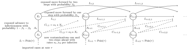
Figure 2: Interpretation of a Poisson INGARCH(2, 2) model as a stochastic epidemic process. Solid lines represent results of multinomial thinning, dashed lines Poisson thinning or imports. Note that the three solid arrows starting at $E_{t}$ do not represent independent thinnings as they are linked by the multinomial distribution and necessarily $L_{t,1}+L_{t,2}+A_{t}=E_{t}$.

3.3 The compound Poisson INGARCH(1, 1) model

A compound Poisson INGARCH(1, 1) process $\{X_{t},t\in\mathbb{Z}\}$ equivalent to (4)–(6) is obtained by extending (9)–(13) to

$$L_{t} =\beta\circ E_{t}$$ (18)

$$A_{t} =E_{t}-L_{t}$$ (19)

$$C_{t} =\kappa\star X_{t}$$ (20)

$$X_{t} =\psi*_{G}(I_{t}+A_{t})$$ (21)

$$E_{t} =L_{t-1}+C_{t-1},$$ (22)

with $E_{0}\sim\text{Pois}(\eta)$. The employed operator $*_{G}$ is defined as

$$\psi*_{G}N=\sum_{i=1}^{N}Z_{i}\ \ \ \text{ with }\ \ \ Z_{i}\stackrel{{\scriptstyle\text{ind}}}{{\sim}}G(\psi)$$

and thus denotes summing over independent samples from a secondary distribution $G(\psi)$. The parameters $\beta$ and $\psi$ as well as the type of the secondary distribution $G$ are shared across the two formulations. The remaining parameters of the original formulation can be recovered as $\nu=\mu_{\psi}(1-\beta)\tau$ and $\ \ \alpha=\mu_{\psi}(1-\beta)\kappa.$ Concerning the initialization, equivalence is achieved by setting $\lambda_{0}=\mu_{\psi}\times\left\{\tau+(1-\beta)\times\eta\right\}$.

The interpretation provided in Section 3.1 can be adapted as follows, see also Figure 3:

• In the extended model $E_{t}$ does not represent exposed individuals, but clusters of exposed individuals. The number of individuals per cluster follows a $G(\psi)$ distribution, and all members of a cluster become infectious simultaneously.

• Imports consist of a $\text{Pois}(\psi)$-distributed number $I_{t}$ of clusters, each of which releases a $G(\psi)$-distributed number of infectives into $X_{t}$.

The biological analogy is somewhat stretched here as in real life one would not expect all members of a cluster to become infectious at the same time. Note that the extension to the compound Poisson setting translates directly to higher-order models as discussed in the previous section, but we omit details.

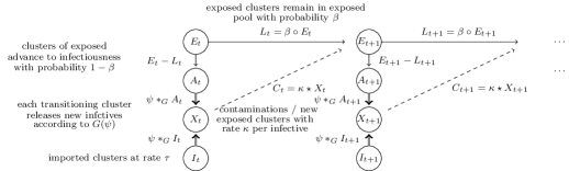
Figure 3: Interpretation of the CP-INGARCH(1, 1) formulation (9)–(13) as a stochastic epidemic process. Solid lines represent results of binomial thinning, dashed lines Poisson thinning, double lines thinning with $*_{G}$. Note that the two solid arrows starting at $E_{t}$ do not represent independent binomial thinnings as by construction $L_{t}+A_{t}=E_{t}$.

4 Derivation of some stochastic properties

We now discuss the derivation of some stochastic properties of the considered models via their reformulation. We focus on the CP-INGARCH(1, 1) model and exploit a link to branching process theory.

4.1 Geometric ergodicity

Fokianos et al [12] showed that a perturbed version of the Poisson INGARCH(1, 1) model is geometrically ergodic and Neumann [22, Theorem 3.1] proved geometric ergodicity of a more general class of Poisson autoregressive models. Ergodicity of various other generalizations has been adressed by several authors [6, 7, 22]. Goncalves et al [13] cover ergodicity (but not geometric ergodicity) of CP-INGARCH models. A proof of geometric ergodicity of the GP-INGARCH(1, 1) model along the lines of [22] has been sketched by Zhu [33]. Higher-order Poisson INGARCH models have been addressed more recently by Neumann [21], while Doukhan et al [23] treat a more general class not limited to conditional Poisson distributions. Mixing properties of non-stationary versions have been considered, too [8].

All of the mentioned contributions can be described as technically involved. As noted by Neumann [22], the difficulty lies in the fact that the process $\{X_{t}\}$ is discrete-valued, while the conditional mean process $\{\lambda_{t}\}$ is real-valued. The re-formulation (18)–(22) of the CP-INGARCH(1, 1) process involves exclusively integer-valued processes, and allows us to exploit results from branching process theory. Substituting $X_{t-1}=\psi*_{G}I_{t}+\psi*_{G}A_{t}$ from equation (21) in (22), $\{E_{t}\}$ can be written as

$$E_{t}=\underbrace{L_{t-1}}_{=\beta\circ E_{t-1}}\ +\ \kappa\star(\psi*_{G}\underbrace{A_{t-1}}_{=E_{t-1}-L_{t-1}})\ +\ \kappa\star(\psi*_{G}I_{t-1}).$$ (23)

Here, $\kappa\star(\psi*_{G}I_{t-1})$ represents exposed clusters caused by imported infections from $t-1$. The term $L_{t-1}$ contains exposed clusters remaining from $E_{t-1}$, while $\kappa\star(\psi*_{G}A_{t-1})$ are new exposed clusters caused by within-community transmission, i.e. by individuals who had been released from the exposed to the infectious pool in $t-1$. Each exposed cluster from $E_{t-1}$ thus contributes to $E_{t}$ in exactly one of two ways. Either it remains in the exposed pool itself, entering $E_{t}$ via $L_{t-1}$, which happens with probability $\beta$. Or, with probability $1-\beta$, it becomes infectious (enters into $A_{t-1}$) and releases a $G(\psi)$-distributed number of newly infectious individuals into $X_{t-1}$. These in turn each contribute new exposed clusters to $E_{t}$ according to a $\text{Pois}(\kappa)$ distribution. Denoting by $B_{k,t-1}$ the number of clusters contributed to $E_{t}$ by the $k$-th of the $E_{t-1}$ clusters from $t-1$, we thus have

$$B_{k,t-1} =\begin{cases}1&\text{with probability }\beta\\ \kappa\star(\psi*_{G}1)&\text{with probability }1-\beta\end{cases}$$ (24)

independently for each $k=1,\dots,E_{t-1}$. Setting

$$I^{*}_{t} =\kappa\star(\psi*_{G}I_{t-1})$$ (25)

we can then re-write recursion (23) as

$$E_{t}=\sum_{k=1}^{E_{t-1}}B_{k,t-1}\ \ +\ \ I^{*}_{t}.$$

Thus, $\{E_{t}\}$ is a Galton-Watson branching process where the offspring distribution (24) is a specific one-inflated compound distribution. The immigration distribution (25) is defined by two compounding steps.

Theory on branching processes with immigration, specifically Theorem 1 from Pakes [24] tells us that $\{E_{t}\}$ is geometrically ergodic if (a) $\mathbb{E}(B_{k,t})<1$, (b) $\mathbb{E}[(B_{k,t})\log(B_{k,t})\ \mid\ B_{k,t}\geq 1]<\infty$, (c) $\mathbb{E}(I^{*}_{t})<\infty$. These conditions are easily verified for $\{E_{t}\}$ provided that $\kappa\mu_{\psi}<1$ and, as previously assumed, $\sigma^{2}_{\psi}<\infty$.

As in Fokianos et al [12], Proposition 1 from Meitz and Saikkonen [20] can then be used to show that geometric ergodicity of $\{E_{t}\}$ is inherited by the joint process $\{(E_{t},L_{t},A_{t},X_{t},C_{t})\}$. Even though it is in principle sufficient to initialize the process with $E_{0}$ and $X_{0}$ as in Section 3.3, we now assume that $\{(E_{t},L_{t},A_{t},X_{t},C_{t})\}$ is initialized by a vector $(e_{0},l_{0},a_{0},x_{0},c_{0})$ with all elements from $\mathbb{N}_{0}$ and $l_{0}+a_{0}=e_{0},x_{0}\geq a_{0}$. Geometric ergodicity of the joint process is then established by verifying two conditions (Assumption 1 in [20]):

1. Given $E_{t}$, $(L_{t},A_{t},X_{t},C_{t})$ is independent of all $E_{u},L_{u},A_{u},X_{u},C_{u},u<t$. It is straightforward to see from equations (18)–(22) or the graphical representation in Figure 3 that this is the case.

2. There is an $n\geq 1$ such that for all $t>n$, the generation mechanism of $E_{t}\ \mid\ E_{0}=e_{0},L_{0}=l_{0},A_{0}=a_{0},X_{0}=x_{0},C_{0}=c_{0}$ has the same structure as that of $E_{t}\ \mid\ E_{n}=\tilde{e}_{n}$, where $\tilde{e}_{n}$ is some function of $(e_{0},l_{0},a_{0},x_{0},c_{0})$. As $(e_{0},l_{0},a_{0},x_{0},c_{0})$ only impacts the further course of the process $\{E_{t}\}$ through $E_{1}=c_{0}+l_{0}$, this is the case for $n=1$.

4.2 Existence of higher moments

Existence of higher-order moments of CP-INGARCH(1, 1) models with time-constant $\psi$ has been proven in [26], but the proof is quite involved. Representation (18)–(22) allows again for a more condensed argument. It is known that if the offspring and immigration distributions of a subcritical Galton-Watson branching process have finite $r$-th moments, this is also the case for the limiting-stationary distribution [17, Sec. 4]. Both conditions are fulfilled for $\{E_{t}\}$ if the $r$-th moment of $G(\psi)$ is finite and $\kappa\mu_{\psi}<1$:

• A randomly stopped sum $Y=\sum_{i=1}^{N}Z_{i}$ of i.i.d. random variables $Z_{i}$ has finite $r$-th moments if $N$ and the $Z_{i}$ have finite $r$-th moments [15, Theorem 5.2]. The Poisson distribution has finite moments of any order. Thus, if the $r$-th moment of $G(\psi)$ is finite, this also holds for $\kappa\star(\psi*_{G}1)$ and thus the offspring distribution from (24).

• Similar arguments imply that if $G(\psi)$ has a finite $r$-th moment, this is also the case for $\psi*_{G}I_{t-1}$ and in a second step the immigration process $I^{*}_{t}=\kappa\star(\psi*_{G}I_{t-1})$ from equation (25).

Consequently, the limiting-stationary distribution of $\{E_{t}\}$ has finite moments up to order $r$ if this is the case for the secondary distribution $G(\psi)$ (while $\kappa\mu_{\psi}<1$). It is then straightforward to show that finiteness of moments translates to $A_{t}=(1-\beta)\circ E_{t}$, $\psi*_{G}A_{t}$ and ultimately $X_{t}=\psi*_{G}I_{t}+\psi*_{G}A_{t}$.

4.3 Approximating the limiting-stationary distribution

As the CP-INGARCH(1, 1) process $\{X_{t}\}$ is ergodic, the limits

$$p_{i}=\lim_{t\rightarrow\infty}\text{Pr}(X_{t}=i\ \mid(e_{0},l_{0},a_{0},x_{0},c_{0}))$$

exist and are independent of the initialization of the process (in the following we therefore suppress the condition in the notation). However, even in the Poisson case no closed form for the $p_{i}$ is known. For the INARCH(1) model, a Markov chain approach can serve to approximate the $p_{i}$ with arbitrary precision [29]. This is based on the fact that the INARCH(1) is a discrete first-order Markov chain so that

$$\text{Pr}(X_{t}=i)=\sum_{j=0}^{\infty}p_{j|i}\times\text{Pr}(X_{t-1}=j).$$

Here, $p_{j|i}=\text{Pr}(X_{t}=i\ |\ X_{t-1}=j)$ is the transition probability from $j$ to $i$. Choosing $T$ sufficiently large, the approximation is given by

$$p_{i}\approx\text{Pr}(X_{T}=i),$$

where $\text{Pr}(X_{T}=i)$ can in turn be approximated by recursively computing

$$\text{Pr}(X_{t}=i)\approx\sum_{j=0}^{M}p_{j|i}\times\text{Pr}(X_{t-1}=j),$$

with sufficiently large support $M$ and some suitable initialization of $X_{0}$ (e.g. starting close to the stationary mean).

This method, however, is not directly applicable to the INGARCH(1, 1) model (4)–(6) as $\{X_{t}\}$ is not a first-order Markov chain. Application to the joint process $\{(X_{T},\lambda_{t})\}$, which is a first-order Markov chain, is not feasible as $\lambda_{t}$ has a continuous support. Formulation (9)–(13), however, enables us to apply the approximation

$$p^{(E)}_{i}\approx\text{Pr}(E_{T}=i)\ \ \text{and}\ \ \text{Pr}(E_{t}=i)\approx\sum_{j=0}^{M}p^{(E)}_{j|i}\times\text{Pr}(E_{t-1}=j)$$

with large $T$ and $M$ to the discrete-valued Markov chain $\{E_{t}\}$. The computation of the transition probabilities $p_{j|i}$ based on recursion (23) is slightly tedious, but without conceptual difficulty. Subsequently one can compute an approximation of the limiting stationary distribution of $X_{t}$ as

$$p_{i}=\sum_{k=0}^{M}p_{k}^{(E)}\times\text{Pr}(X_{t}=i\ \mid\ E_{t}=k).$$

Appendix A Equivalence of the classical and thinning-based INGARCH formulations

A.1 Poisson INGARCH(1, 1)

We demonstrate that the process $\{X_{t},t\in\mathbb{N}_{0}\}$ from (9)–(13) is equivalent to the Poisson INGARCH(1, 1) process (1)–(2). We start by decomposing $C_{t},t\in\mathbb{N}_{0}$ and $E_{0}$ by when these exposed individuals will become infectious. We denote by $C_{t}^{(i)}$ the number of exposed persons caused by infectives from time $t$ and turning themselves infectious at $t+i$; and by $E^{(i)}_{0}$ the number of exposed individuals initially in the pool and turning infectious at time $i$ (note that $C_{t}^{(i)}$ is not to be confused with $C_{t,i}$ from Section 3.2). This implies

$$A_{t}=\sum_{i=1}^{t}C_{t-i}^{(i)}\ \ +\ \ E_{0}^{(t)}.$$ (26)

for $t\geq 1$. A person contaminated by an infective from time $t$ (entering the exposed pool at time $t+1$) has a probability of

$$\beta^{i-1}(1-\beta)$$ (27)

to become infectious at time $t+i,i=1,2,\dots$, and thus be part of $C_{t}^{(i)}$ (it has to remain in the exposed pool $i-1$ times and then turn infectious). The Poisson splitting property [16] then implies that given $X_{t}$, the $C_{t}^{(i)},i=1,2,\dots$ are independently Poisson distributed,

$$C_{t}^{(i)}\mid X_{t}\stackrel{{\scriptstyle\text{ind}}}{{\sim}}\text{Pois}(\beta^{i-1}[1-\beta]\kappa X_{t}),i=1,2,\dots$$

We note that given $X_{t}$, $C_{t}^{(i)}$ does not have any impact on the further course of the process $\{X_{t}\}$ until time $t+i$. Also, given $X_{t}$, $C_{t}^{(i)}$ is independent of all preceding values $X_{t-1},X_{t-2},X_{0}$. We can thus extend the condition in the above and write

$$C_{t}^{(i)}\mid X_{t+i-1},\dots,X_{0}\sim\text{Pois}(\beta^{i-1}[1-\beta]\kappa X_{t}).$$ (28)

Moreover, again because, given $X_{t}$, $C_{t}^{(i)}$ only impacts the further process from $t+i$ onwards, it is clear that $C_{t}^{(i)}\perp C_{u}^{(j)}\mid X_{t+i-1},X_{t+i-2},\dots,X_{0}$ if $u<t+i$.

Now consider

$$X_{t} =I_{t}\ \ +\ \ \underbrace{\sum_{i=1}^{t}C_{t-i}^{(i)}\ \ +\ \ E_{0}^{(t)}}_{=A_{t}},$$ (29)

where we substituted $A_{t}$ in equation (12) using equation (26). In analogy to the above argument, $E_{0}^{(t)}$ is Poisson distributed with rate $\beta^{t}(1-\beta)\eta$ and independent of all $X_{u}$ and $C_{u}^{(i)},u\leq t-1$. Conditioned on $X_{t-1},\dots,X_{0}$, we thus have that $X_{t}$ is a sum of independent Poisson random variables. This implies

$$X_{t}\mid X_{t-1},\dots,X_{0}\sim\text{Pois}(\lambda_{t})$$

where the conditional expectation is given by

$$\lambda_{t}=\mathbb{E}(I_{t})\ \ +\ \ \sum_{i=1}^{t}\mathbb{E}(C_{t-i}^{(i)}\ \mid\ X_{t-1},\dots,X_{0})\ \ +\ \ \mathbb{E}(E_{0}^{(t)})$$

$$\ \ \ =\ \ \tau\ \ \ \ \ +\ \ \sum_{i=1}^{t}\beta^{i-1}(1-\beta)\kappa X_{t-i}\ \ \ \ \ \ \ \ \ \ +\ \ \beta^{t}(1-\beta)\eta.$$

We can then re-write $\lambda_{t}$ as

$$\lambda_{t} =(1-\beta)\tau+(1-\beta)\kappa X_{t-1}+\beta\left\{\tau+\sum_{i=2}^{t}\beta^{i-1}(1-\beta)\kappa X_{t-i}\ \ +\ \ \beta^{t-1}(1-\beta)\eta\right\}$$

$$=\underbrace{(1-\beta)\tau}_{\nu}\ +\ \underbrace{(1-\beta)\kappa}_{\alpha}X_{t-1}\ +\ \beta\lambda_{t-1}$$

for $t\geq 2$. This is the form a Poisson INGARCH(1, 1) model. We conclude by considering the initialization of the process, where we have

$$\lambda_{1}=\mathbb{E}(X_{1}\ \mid\ X_{0}) =\tau+(1-\beta)\kappa X_{0}+\beta(1-\beta)\eta$$

$$=(1-\beta)\tau+(1-\beta)\kappa X_{0}+\beta\left\{\tau+(1-\beta)\times\eta\right\},$$

meaning that we have to set $\lambda_{0}=\tau+(1-\beta)\times\eta$ for initialization. The proofs for the INGARCH($p,q$) and CP-INGARCH(1, 1) models follow the same structure and have been moved to the Supplementary Material for space reasons.

Appendix B Supplementary material

B.1 Demonstration of equivalence for the INGARCH($p,q$) model

We use an argument similar to the one from Section A.1 to demonstrate that the classical formulation (1), (3) of the INGARCH($p,q$) model and the thinning-based version (14)–(17) are equivalent. Again we denote by $C_{t}^{(i)},i=1,2,\dots$ the number of persons contaminated by infectives from time $t$ and becoming themselves infectious at $t+i$. Extending on the notation from the Poisson INGARCH(1, 1) case, we denote by $E^{(i)}_{m},m=1-q,\dots,0,i=1,2,\dots$ the number of individuals entering the exposed pool via the initialization at time $m$ and turning infectious at time $m+i$. Generalizing equation (29) we then have

$$X_{t}=I_{t}\ \ +\ \ \underbrace{\sum_{i=1}^{t+p-1}C_{t-i}^{(i)}\ \ +\ \ \sum_{m=1-q}^{0}E_{m}^{(t-m)}}_{=A_{t}},$$

for $t=1,2,\dots$. Arguments identical to those from the previous section imply that given $X_{t-1},\dots,X_{1-p}$ all summands in the above equation are independently Poisson distributed, so that $X_{t}$, too, is conditionally Poisson with a rate $\lambda_{t}$.

Paralleling equation (28), the conditional expectation of $C_{t}^{(i)}$ is given by

$$\mathbb{E}(C_{t}^{(i)}\ \mid\ X_{t+i-1},\dots,X_{1-p})=\left(1-\sum_{l=1}^{q}\beta_{l}\right)\times\left(\sum_{k=1}^{p}\ \kappa_{k}\pi_{i-k}\right)X_{t},$$ (30)

where we denote by $\pi_{j}$ the probability that an individual entering the exposed pool at time $t$ is also in the pool at time $t+j$. The reasoning behind this relationship is that the $X_{t}$ infectives from time $t$ generate exposures entering at times $t+1,\dots,t+p$ with rates $\kappa_{1},\dots,\kappa_{p}$, respectively. The exposed individuals then have to also be present in the exposed pool exactly $i-1,\dots,i-p$ time points later, respectively (which happens with probabilities $\pi_{i-1},\dots,\pi_{i-p}$), and then leave it (which happens with probability $1-\sum_{l=1}^{q}\beta_{l}$).

For the $\pi_{j}$, the recursion

$$\pi_{j}=\sum_{l=1}^{q}\beta_{l}\pi_{j-l},$$ (31)

with $\pi_{0}=1$ and $\pi_{k}=0$ for $k<0$ holds. This is because an individual which entered the exposed pool at time $t$ can arrive in $E_{t+j},j\geq 1$ by a move from any of $E_{t+j-1},\dots E_{t+j-q}$ (even though some of these moves may not be possible if $j<q$; this will be reflected in $\pi_{j-l}=0$). To do so, the individual needs to have arrived at the respective $E_{t+j-l}$ (which it does with probability $\pi_{j-l}$) and then make an $l$-step jump into $E_{t+j}$ (this happens with probability $\beta_{l}$).

We can now consider

$$\lambda_{t}=\mathbb{E}(X_{t}\ \mid\ X_{t-1},\dots,X_{1-p})= \ \tau\ +\ \sum_{i=1}^{t+p-1}\mathbb{E}(L^{(i)}_{t-i}\ \mid\ X_{t-1},\dots,X_{1-p})\ +\sum_{m=1-q}^{0}\mathbb{E}(E_{m}^{(t+m)}\ \mid\ X_{t-1},\dots,X_{1-p}).$$ (32)

Focusing on the second summand and plugging in equation (30), we obtain

$$\sum_{i=1}^{t+p-1}\mathbb{E}(L^{(i)}_{t}\ \mid\ X_{t-1},\dots,X_{1-p})= \left(1-\sum_{l=1}^{q}\beta_{l}\right)\times\left(\sum_{i=1}^{t+p-1}\sum_{k=1}^{p}\kappa_{k}\pi_{i-k}X_{t-i}\right)$$

$$= \left(1-\sum_{l=1}^{q}\beta_{l}\right)\times\left(\sum_{k=1}^{p}\sum_{i=k}^{t+p-1}\kappa_{k}\pi_{i-k}X_{t-i}\right).$$

Note that in the last step we can start the last sum from $i=k$ rather than $i=1$ as $\pi_{i-k}=0$ for $i<k$. We can then further decompose this sum into

$$= \left(1-\sum_{l=1}^{q}\beta_{l}\right)\times\left(\underbrace{\sum_{k=1}^{p}\kappa_{k}\pi_{0}X_{t-k}}_{\text{corresponds to }i=k;\text{ note: }\pi_{0}=1}\ +\ \sum_{k=1}^{p}\sum_{i=k+1}^{t+p-1}\kappa_{k}\pi_{i-k}X_{t-i}\right)$$

$$= \left(1-\sum_{l=1}^{q}\beta_{l}\right)\times\left\{\sum_{k=1}^{p}\kappa_{k}X_{t-k}\ +\ \sum_{k=1}^{p}\sum_{i=k+1}^{t+p-1}\kappa_{k}\times\underbrace{\left(\sum_{j=1}^{q}\beta_{j}\pi_{i-k-j}\right)}_{\text{using equation \eqref{eq:recursion_pi}}}\times X_{t-i}\right\}$$

$$= \left(1-\sum_{l=1}^{q}\beta_{l}\right)\times\left\{\sum_{k=1}^{p}\kappa_{k}X_{t-k}\ +\ \sum_{j=1}^{q}\beta_{j}\times\left(\sum_{k=1}^{p}\sum_{i=k+1}^{t+p-1}\kappa_{k}\times\pi_{i-k-j}\times X_{t-i}\right)\right\}$$

$$= \left(1-\sum_{l=1}^{q}\beta_{l}\right)\times\left\{\sum_{k=1}^{p}\kappa_{k}X_{t-k}\ +\ \sum_{j=1}^{q}\beta_{j}\times\left(\sum_{k=1}^{p}\sum_{i=k+1-j}^{(t-j)+p-1}\kappa_{k}\times\pi_{i-k}\times X_{(t-j)-i}\right)\right\}$$

$$= \left(1-\sum_{l=1}^{q}\beta_{l}\right)\times\left\{\sum_{k=1}^{p}\kappa_{k}X_{t-k}\ +\ \sum_{j=1}^{q}\beta_{j}\times\left(\sum_{k=1}^{p}\sum_{i=1}^{(t-j)+p-1}\kappa_{k}\times\pi_{i-k}\times X_{(t-j)-i}\right)\right\}$$ (33)

where in the last step we can let the last sum start at $i=1$ rather than $i=k+1-j$ as $\pi_{i-k}=0$ for $i=1,\dots,k-j$.

For the third term from equation (32) we pursue a similar recursive argument:

$$\sum_{m=1-q}^{0}\mathbb{E}(E_{m}^{(t+m)}\ \mid\ X_{t-1},\dots,X_{1-p}) =\left(1-\sum_{l=1}^{q}\beta_{l}\right)\times\sum_{m=1-q}^{0}\pi_{t-m}\rho_{m}$$

$$=\left(1-\sum_{l=1}^{q}\beta_{l}\right)\times\sum_{m=1-q}^{0}\sum_{j=1}^{q}\beta_{j}\pi_{t-j-m}\rho_{m}$$

$$=\left(1-\sum_{l=1}^{q}\beta_{l}\right)\times\sum_{j=1}^{q}\beta_{j}\times\left(\sum_{m=1-q}^{0}\pi_{(t-j)-m}\rho_{m}\right).$$ (34)

Plugging the terms from (33) and (34) into (32) we then get

$$\lambda_{t}= \ \ \tau\ +\ \left(1-\sum_{l=1}^{q}\beta_{l}\right)\times\Bigg{\{}\sum_{k=1}^{p}\kappa_{k}X_{t-k}\ +\ \sum_{j=1}^{q}\beta_{j}\times\left(\sum_{k=1}^{p}\sum_{i=1}^{(t-j)+p-1}\kappa_{k}\times\pi_{i-k}\times X_{(t-j)-i}\right)$$

$$\ \ \ \ \ \ \ \ \ \ \ \ \ \ \ \ \ \ \ \ \ \ \ \ \ \ \ \ \ \ \ \ \ +\ \sum_{j=1}^{q}\beta_{j}\times\left(\sum_{m=1-q}^{0}\pi_{(t-j)-m}\rho_{m}\right)\Bigg{\}}.$$

This can be re-ordered to

$$\lambda_{t} =\left(1-\sum_{l=1}^{q}\beta_{l}\right)\times\tau\ +\ \left(1-\sum_{l=1}^{q}\beta_{l}\right)\times\left(\sum_{k=1}^{p}\kappa_{k}X_{t-k}\right)$$

$$\ \ \ +\sum_{j=1}^{q}\beta_{j}\underbrace{\left\{\tau\ +\ \left(1-\sum_{l=1}^{q}\beta_{l}\right)\times\left(\sum_{k=1}^{p}\sum_{i=1}^{(t-j)+p-1}\kappa_{k}\times\pi_{i-k}\times X_{(t-j)-i}\right)\ +\ \left(1-\sum_{l=1}^{q}\beta_{l}\right)\times\left(\sum_{m=1-q}^{0}\pi_{(t-j)-m}\rho_{m}\right)\right\}}_{=\lambda_{t-j}}$$

$$=\nu\ \ +\ \ \sum_{k=1}^{p}\alpha_{k}X_{t-k}\ \ +\ \ \sum_{j=1}^{q}\beta_{j}\lambda_{t-j},$$

where

$$\nu=\left(1-\sum_{l=1}^{q}\beta_{l}\right)\times\tau,\ \ \ \alpha_{k}=\left(1-\sum_{l=1}^{q}\beta_{l}\right)\times\kappa_{k},k=1,\dots,p.$$

This is the form of a Poisson INGARCH($p,q$) model as defined in equation (3). Concerning the initialization, it can be shown that one needs to set $\lambda_{m}=(1-\sum_{j=1}^{q}\beta_{j})\times\eta_{m},m=1-q,\dots,0$. This can be done using essentially the same argument as in Section A.1, but we omit the somewhat lengthy details.

B.2 Compound Poisson INGARCH(1, 1)

Setting $N_{t}=I_{T}+A_{t}$, the same arguments as in (A.1) can be used to show that

$$N_{t}\mid X_{t-1},\dots,X_{0}\sim\text{Pois}(\lambda_{t}/\mu_{\psi})$$

where the conditional expectation is given by

$$\lambda_{t}/\mu_{\psi}=\mathbb{E}(I_{t})\ \ +\ \ \sum_{i=1}^{t}\mathbb{E}(C_{t-i}^{(i)})\ \ +\ \ \mathbb{E}(E_{0}^{(t)})$$

$$\ \ \ \ \ \ \ \ =\tau\ \ +\ \ \sum_{i=1}^{t}\beta^{i-1}(1-\beta)\kappa X_{t-i}\ \ +\ \ \beta^{t}(1-\beta)\eta$$

$$\Leftrightarrow\ \ \lambda_{t}=\mu_{\psi}\tau\ \ +\ \ \mu_{\psi}\times\sum_{i=1}^{t}\beta^{i-1}(1-\beta)\kappa X_{t-i}\ \ +\ \ \mu_{\psi}\beta^{t}(1-\beta)\eta$$

We can then re-write $\lambda_{t}$ as

$$\lambda_{t} =\mu_{\psi}(1-\beta)\tau+\mu_{\psi}(1-\beta)\kappa X_{t-1}+\beta\left[\mu_{\psi}\tau+\mu_{\psi}\sum_{i=2}^{t}\beta^{i-1}(1-\beta)\kappa X_{t-i}\ \ +\ \ \mu_{\psi}\beta^{t-1}(1-\beta)\eta\right]$$

$$=\underbrace{\mu_{\psi}(1-\beta)\tau}_{\nu}\ +\ \underbrace{\mu_{\psi}(1-\beta)\kappa}_{\alpha}X_{t-1}\ +\ \beta\lambda_{t-1}$$

for $t\geq 2$. Combined with the relationship $X_{t}=\psi*_{G}(I_{t}+A_{t})=\psi*_{G}N_{t}$ this is the form a CP-INGARCH(1, 1) model as introduced in (4)–(6). Concerning the initialization of the process, the same argument as in Section 3.1 implies that we have to set $\lambda_{0}=\mu_{\psi}\times\left\{\tau+(1-\beta)\times\eta\right\}$.

References

- [1] M.A. Al-Osh and A.A. Alzaid. First-order integer-valued autoregressive (INAR(1)) process. Journal of Time Series Analysis, 8(3):261–275, 1987.
- [2] A. A. Alzaid and M. Al-Osh. An integer-valued pth-order autoregressive structure (INAR(p)) process. Journal of Applied Probability, 27(2):314–324, 1990.
- [3] C. Bauer and J. Wakefield. Stratified space–time infectious disease modelling, with an application to hand, foot and mouth disease in China. Journal of the Royal Statistical Society: Series C (Applied Statistics), 67(5):1379–1398, 2018.
- [4] J. Bracher. A new INARMA(1, 1) model with Poisson marginals. In A. Steland, E. Rafajłowicz, and O. Okhrin, editors, Stochastic Models, Statistics and Their Applications, pages 323–333. Springer, 2019.
- [5] T. Britton and E. Pardoux. Stochastic Epidemic Models with Inference. Springer, 2019.
- [6] R.A. Davis and H. Liu. Theory and inference for a class of nonlinear models with application to time series of counts. Statistica Sinica, 26(4):1673–1707, 2016.
- [7] R. Douc, P. Doukhan, and E. Moulines. Ergodicity of observation-driven time series models and consistency of the maximum likelihood estimator. Stochastic Processes and their Applications, 123(7):2620 – 2647, 2013.
- [8] P. Doukhan, A. Leucht, and M. H. Neumann. Mixing properties of non-stationary INGARCH(1,1) processes, 2021.
- [9] W Feller. An Introduction to Probability Theory and Its Applications, Volume 1. Wiley, 1968.
- [10] R. Ferland, A. Latour, and D. Oraichi. Integer-valued GARCH process. Journal of Time Series Analysis, 27(6):923–942, 2006.
- [11] K. Fokianos. Handbook of Discrete-Valued Time Series, chapter Statistical Analysis of Count Time Series Models: A GLM Perspective, pages 3–24. Chapman and Hall/CRC, 2016.
- [12] K. Fokianos, A. Rahbek, and D. Tjøstheim. Poisson autoregression. Journal of the American Statistical Association, 104(488):1430–1439, 2009.
- [13] E. Gonçalves, N. Mendes-Lopes, and F. Silva. Infinitely divisible distributions in integer-valued GARCH models. Journal of Time Series Analysis, 36(4):503–527, 2015.
- [14] E. Gonçalves, N. Mendes-Lopes, and F. Silva. A new approach to integer-valued time series modeling: The Neyman type-A INGARCH model. Lithuanian Mathematical Journal, 55(2):231–242, 2015.
- [15] A. Gut. Stopped Random Walks - Limit Theorems and Applications. Springer, 2009.
- [16] J.F.C. Kingman. Poisson Processes. Oxford University Press, Oxford, United Kingdom, 1993.
- [17] K. Lange, M. Boehnke, and R. Carson. Moment computations for subcritical branching processes. Journal of Applied Probability, 18(1):52–64, 1981.
- [18] Yang Lu. The predictive distributions of thinning-based count processes. Scandinavian Journal of Statistics, 48(1):42–67, 2021.
- [19] E. McKenzie. Some simple models for discrete variate time series. Journal of the American Water Resources Association, 21(4):645–650, 1985.
- [20] M. Meitz and P. Saikkonen. Ergodicity, mixing, and existence of moments of a class of Markov models with applications to GARCH and ACD models. Econometric Theory, 24(5):1291–1320, 2008.
- [21] M. H. Neumann. Bootstrap for integer-valued GARCH(p, q) processes. Statistica Neerlandica, 75(3):343–363, 2021.
- [22] M.H. Neumann. Absolute regularity and ergodicity of Poisson count processes. Bernoulli, 17(4):1268–1284, 11 2011.
- [23] Doukhan P, Mamode Khan N, and Neumann M. Mixing properties of integer-valued GARCH processes. ALEA – Latin American Journal of Probability and Mathematical Statistics, 18:401–420, 2021.
- [24] A.G. Pakes. Branching processes with immigration. Journal of Applied Probability, 8(1):32–42, 1971.
- [25] M.G. Scotto, C.H. Weiß, and S. Gouveia. Thinning-based models in the analysis of integer-valued time series: a review. Statistical Modelling, 15(6):590–618, 2015.
- [26] F. Silva. Compound-Poisson Integer-Valued GARCH Processes. PhD thesis, University of Coimbra, 2016.
- [27] F. W. Steutel and K. van Harn. Discrete analogues of self-decomposability and stability. The Annals of Probability, 7(5):893–899, 1979.
- [28] C.H. Weiß. An Introduction to Discrete-Valued Time Series. Wiley, Hoboken, NJ, 2018.
- [29] C.H. Weiß. The INARCH(1) model for overdispersed time series of counts. Communications in Statistics - Simulation and Computation, 39(6):1269–1291, 2010.
- [30] C.H. Weiß. A Poisson INAR(1) model with serially dependent innovations. Metrika, 78(7):829–851, 2015.
- [31] C.H. Weiß, Gonçalves E., and Lopes N.M. Testing the compounding structure of the CP-INARCH model. Metrika, 80(5):571–603, 2017.
- [32] H.Y. Xu, M. Xie, T.N. Goh, and X. Fu. A model for integer-valued time series with conditional overdispersion. Computational Statistics & Data Analysis, 56(12):4229 – 4242, 2012.
- [33] F. Zhu. Modeling overdispersed or underdispersed count data with generalized Poisson integer-valued GARCH models. Journal of Mathematical Analysis and Applications, 389(1):58 – 71, 2012.