On a class of interpolation inequalities on the 2D sphere

Abstract.

We prove estimates for the $L^{p}$-norms of systems of functions and divergence free vector functions that are orthonormal in the Sobolev space $H^{1}$ on the 2D sphere. As a corollary, order sharp constants in the embedding $H^{1}\hookrightarrow L^{q}$, $q<\infty$, are obtained in the Gagliardo–Nirenberg interpolation inequalities.

1. Introduction

The following interpolation inequality holds on the sphere $\mathbb{S}^{d}$ (see [1] and also [2]):

$$\frac{q-2}{d}\int_{\mathbb{S}^{d}}|\nabla\varphi|^{2}d\mu+\int_{\mathbb{S}^{d}}|\varphi|^{2}d\mu\geq\left(\int_{\mathbb{S}^{d}}|\varphi|^{q}d\mu\right)^{2/q}.$$ (1.1)

Here $d\mu$ is the normalized Lebesgue measure on $\mathbb{S}^{d}$:

$$d\mu=\frac{d\sigma}{\sigma_{d}}=\frac{d\sigma}{\frac{2\pi^{\frac{d+1}{2}}}{\Gamma(\frac{d+1}{2})}}\,,$$

so that $\mu(\mathbb{S}^{d})=1$ (the gradient is calculated with respect to the natural metric). Next, $q\in[2,\infty)$ for $d=1,2$, and $q\in[2,2d/(d-2)]$ for $d\geq 3$. The remarkable fact about (1.1) is that the constant $(q-2)/d$ is sharp for all admissible $q$. The inequality clearly degenerates and turns into equality on constants. The fact that the constant $(q-2)/d$ is sharp is verified by means of the sequence $\varphi_{\varepsilon}(s)=1+\varepsilon v(s)$ as $\varepsilon\to 0$, where $v(s)$ is an eigenfunction of the Laplacian on $\mathbb{S}^{d}$ corresponding to the first positive eigenvalue $d$, see [3] and the references therein.

However, in applications (for instance, for the Navier–Stokes equations on the 2D sphere) the functions $\varphi$ usually play the role of stream functions of a divergence free vector functions $u$, $u=\nabla^{\perp}\varphi$, and therefore without loss of generality $\varphi$ can be chosen to be orthogonal to constants.

In this work we consider the two-dimensional sphere $\mathbb{S}^{2}$ only and are interested in writing the Sobolev embedding $H^{1}(\mathbb{S}^{2})\hookrightarrow L^{q}(\mathbb{S}^{2})$ as a multiplicative inequality of Gagliardo–Nirenberg type involving the $L^{2}$-norms of $\varphi$ and $\nabla\varphi$ on right-hand side: $\|\varphi\|_{L^{2}(\mathbb{S}^{2})}=:\|\varphi\|$ and $\|\nabla\varphi\|_{L^{2}(\mathbb{S}^{2})}=:\|\nabla\varphi\|$.

It is also well known that in the case of $\mathbb{R}^{d}$ interpolation inequalities in the additive form and in the multiplicative form are equivalent and the passage from the former to the latter is realized by the introduction of the parameter $m$ in the inequality (by scaling $x\to mx$) and subsequent minimization with respect to $m$. To go other way round one can use Young’s inequality (with parameter) for products to obtain the interpolation inequality in the additive form.

This scheme obviously does not work on a manifold due to the lack of scaling. One possible way to introduce a parameter in the Sobolev inequality is to consider the Sobolev space $H^{1}$ with norm and scalar product

$$\|\varphi\|_{H^{1}}^{2}:=m^{2}\|\varphi\|^{2}+\|\nabla\varphi\|^{2},\quad(\varphi_{1},\varphi_{2})_{H^{1}}:=m^{2}(\varphi_{1},\varphi_{2})+(\nabla\varphi_{1},\nabla\varphi_{2})$$

depending on a parameter $m>0$, and then to trace down the explicit dependence of the embedding constant on $m$. In this work this is done in much more general framework of the inequalities for $H^{1}$-orthonormal families proved in [4].

We can now state and discuss our main result.

Theorem 1.1.

Let a family of zero mean functions $\{\varphi_{j}\}_{j=1}^{n}\in\dot{H}^{1}(\mathbb{S}^{2})$ be orthonormal with respect to the scalar product

$$m^{2}(\varphi_{i},\varphi_{j})+(\nabla\varphi_{i},\nabla\varphi_{j})=\delta_{ij}.$$ (1.2)

Then for $1\leq p<\infty$ the function

$$\rho(x):=\sum_{j=1}^{n}|\varphi_{j}(x)|^{2}$$

satisfies the inequality

$$\|\rho\|_{L^{p}}\leq\mathrm{B}_{p}m^{-2/p}n^{1/p},$$ (1.3)

where

$$\mathrm{B}_{p}\leq\left(\frac{p-1}{4\pi}\right)^{(p-1)/p}.$$ (1.4)

These inequalities were proved in the case of $\mathbb{R}^{d}$ in [4] for $p=\infty$ ($d=1$), $1\leq p<\infty$ ($d=2$), and for the critical $p=d/(d-2)$ ($d\geq 3$). No expressions for the constants were given, the dependence on $m$ is again uniquely defined by scaling, and the main interest there was in the dependence of the right hand side on $n$.

For $p=2$ this inequality has played an essential role in finding explicit optimal bounds for the attractor dimension for the damped regularized Euler–Bardina–Voight system for various boundary conditions both in the two and three dimensional cases, see [5, 6, 7]. More precisely, it was shown in [5, 7] that $\mathrm{B}_{2}\leq(4\pi)^{-1/2}$ for $\mathbb{T}^{2}$, $\mathbb{S}^{2}$, and $\mathbb{R}^{2}$ based on the following two inequalities for the lattice sum over $\mathbb{Z}^{2}_{0}=\mathbb{Z}^{2}\setminus\{0,0\}$ and the series with respect to the spectrum of the Laplacian on $\mathbb{S}^{2}$ that were proved there for the special case, when $p=2$

$$J_{p}(m):=\frac{(p-1)m^{2(p-1)}}{\pi}\sum_{n\in{\mathbb{Z}}_{0}^{2}}\frac{1}{(m^{2}+|n|^{2})^{p}}<1,$$ (1.5)

$$I_{p}(m):=m^{2(p-1)}(p-1)\sum_{n=1}^{\infty}\frac{2n+1}{\bigl{(}m^{2}+n(n+1)\bigr{)}^{p}}<1.$$ (1.6)

The case $p=2$ is not at all specific in the general scheme of the proof of Theorem 1.1 and the general case in the theorem both for $\mathbb{T}^{2}$ and $\mathbb{S}^{2}$ immediately follows once we have inequality (1.5), (1.6) for all $1<p<\infty$.

Inequality (1.5) and therefore Theorem 1.1 for the torus $\mathbb{T}^{2}$ has recently been proved in [8], and the main result of this work is the proof of (1.6) and Theorem 1.1 for the sphere.

We point out that in the case of $\mathbb{R}^{2}$, instead of (1.5) and (1.6) we simply have the equality

$$\frac{(p-1)m^{2(p-1)}}{\pi}\int_{\mathbb{R}^{2}}\frac{dx}{(m^{2}+|x|^{2})^{p}}=1.$$ (1.7)

For one function ($n=1$) Theorem 1.1 is equivalent to the Sobolev inequality with parameter $H^{1}\hookrightarrow L^{q}$, $q=2p\in[2,\infty)$, which can equivalently be written as a Gagliardo–Nirenberg inequality

$$\|f\|_{L^{q}}\leq\left(\frac{1}{4\pi}\right)^{(q-2)/2q}\left(\frac{q}{2}\right)^{1/2}\|f\|^{2/q}\|\nabla f\|^{1-2/q},$$ (1.8)

which holds for $\mathbb{R}^{2}$, $\mathbb{T}^{2}$ and $\mathbb{S}^{2}$, see Corollary 2.1.

For the torus $\mathbb{T}^{2}$ inequality (1.8) can be proved in a direct way [8] by using the Hausdorff–Young inequality for the discrete Fourier series and again estimate (1.5). In the case of $\mathbb{R}^{2}$ this approach is well known and with the additional use of the Babenko–Beckner inequality [9, 10] for the Fourier transform (and equality (1.7)) gives the following improvement of inequality (1.8) for $\mathbb{R}^{2}$ with the best to date closed form estimate for the constant [11]:

$$\|\varphi\|_{L^{q}(\mathbb{R}^{2})}\leq\left(\frac{1}{4\pi}\right)^{\frac{q-2}{2q}}\frac{q^{(q-2)/q}}{(q-1)^{(q-1)/q}}\left(\frac{q}{2}\right)^{1/2}\|\varphi\|^{2/q}\|\nabla\varphi\|^{1-2/q},\ q\geq 2,$$ (1.9)

see also [12, Theorem 8.5] where the equivalent result is obtained for the inequality in the additive form.

Of course, inequality (1.9) for $\mathbb{R}^{2}$ and inequality (2.4) for $\mathbb{T}^{2}$ both are a special case of Gagliardo–Nirenberg inequality. For $\mathbb{R}^{2}$ the best constant is known for every $q\geq 2$ and is expressed in terms of a norm of the ground state solution of the corresponding nonlinear Euler–Lagrange equation [13]. However, not in the explicit form. As mentioned above, inequality (1.9) was known before, while inequality (2.4) (more precisely, the estimate for the constant in it) for the torus $\mathbb{T}^{2}$ was recently obtained in [8].

As far as the case of the sphere $\mathbb{S}^{2}$ is concerned we do not know how to prove (1.8) in a way other than the one function corollary of the general Theorem 1.1. The main difference from the case of $\mathbb{T}^{2}$ is that the orthonormal spherical functions are not uniformly bounded in $L^{\infty}$.

Our approach makes it possible to prove similar inequalities in the vector case. Namely, we show that for $u\in\mathbf{H}^{1}_{0}(\Omega)\cap\{\mathop{\mathrm{missing}}{div}u=0\}$ it holds

$$\|u\|_{L_{q}(\mathbb{S}^{2})}\leq\left(\frac{1}{4\pi}\right)^{(q-2)/2q}\left(\frac{q}{2}\right)^{1/2}\|u\|^{2/q}\|\operatorname{rot}u\|^{1-2/q}.$$

Here $\Omega\subseteq\mathbb{S}^{2}$ is an arbitrary domain on $\mathbb{S}^{2}$. This inequality looks very similar to (1.8), the important difference being that, unlike the scalar case, the vector Laplacian on $\mathbb{S}^{2}$ is positive definite, and we can freely use the extension by zero.

Finally, it is natural to compare inequalities (1.1) with $d=2$ and (1.8) for functions with mean value zero. To do so we go over to the natural measure on $\mathbb{S}^{2}$ in (1.1) and then use the Poincare inequality $\|\varphi\|^{2}\leq 2^{-1}\|\nabla\varphi\|^{2}$ to obtain:

$$\|\varphi\|_{L^{q}(\mathbb{S}^{2})}\leq\left(\frac{1}{4\pi}\right)^{(q-2)/2q}\left(\frac{q-2}{2}\|\nabla\varphi\|^{2}+\|\varphi\|^{2}\right)^{1/2}\leq$$

$$\leq\left(\frac{1}{4\pi}\right)^{(q-2)/2q}\left(\frac{q-1}{2}\right)^{1/2}\|\nabla\varphi\|,$$

while (1.8) gives

$$\|\varphi\|_{L_{q}(\mathbb{S}^{2})}\leq\left(\frac{1}{4\pi}\right)^{(q-2)/2q}\left(\frac{q}{2}\right)^{1/2}\frac{1}{2^{1/q}}\|\nabla\varphi\|.$$

The constant here is marginally smaller, since

$$2^{-2/q}\leq 1-1/q,\quad q\geq 2.$$

Since inequality (1.1) turns into equality on constants, this inequality may not be sharp on the subspace of zero mean functions on $\mathbb{S}^{2}$, and the constant in (1.8) is not sharp. However, looking at (1.8) and (1.9) for $\mathbb{T}^{2}$, $\mathbb{S}^{2}$ and for $\mathbb{R}^{2}$, respectively, one can suggest that that the sharp constant here is

$$\mathrm{c}_{q}\sim\left(\frac{1}{8\pi}\right)^{1/2}\,q^{1/2}\quad\text{as}\quad q\to\infty.$$

The expression on the right-hand side here curiously coincides with sharp constant in the Sobolev inequality for the limiting exponent, see [14, 15]:

$$\|\varphi\|_{L^{q}({\mathbb{R}^{d}})}\leq\frac{\sqrt{q}}{d\sqrt{2\pi}}\left[\frac{\Gamma(d)}{\Gamma(d/2)}\right]^{1/d}\|\nabla\varphi\|_{L^{2}({\mathbb{R}^{d}})},\qquad\frac{1}{q}=\frac{1}{2}-\frac{1}{d},$$

if we formally set $d=2$. Of course, this inequality does hold in $\mathbb{R}^{2}$, since $d\geq 3$ in it.

Theorem 1.1 and the similar result in the vector case are proved in the next Section 2, and the key estimate for the series (1.6) is proved in Section 3.

2. Proof of the main result

Proof of Theorem 1.1.

We first recall the basic facts concerning the spectrum of the scalar Laplace operator $\Delta=\mathop{\mathrm{missing}}{div}\nabla$ on the sphere $\mathbb{S}^{2}$ (see, for instance, [16]):

$$-\Delta Y_{n}^{k}=n(n+1)Y_{n}^{k},\quad k=1,\dots,2n+1,\quad n=0,1,2,\dots.$$ (2.1)

Here the $Y_{n}^{k}$ are the orthonormal real-valued spherical harmonics and each eigenvalue $\Lambda_{n}:=n(n+1)$ has multiplicity $2n+1$.

The following identity is essential in what follows: for any $s\in\mathbb{S}^{2}$

$$\sum_{k=1}^{2n+1}Y_{n}^{k}(s)^{2}=\frac{2n+1}{4\pi}.$$ (2.2)

Since inequality (1.3) with (1.4) clearly holds for $p=1$ we assume below that $1<p<\infty$. Let us define two operators

$$\mathbb{H}=V^{1/2}(m^{2}-{\Delta})^{-1/2}\Pi,\quad\mathbb{H}^{*}=\Pi(m^{2}-{\Delta})^{-1/2}V^{1/2},$$ (2.3)

where $V\in L^{p}$, is a non-negative scalar function and $\Pi$ is the projection onto the space of functions with mean value zero:

$$\Pi\varphi=\varphi-\frac{1}{4\pi}\int_{\mathbb{S}^{2}}\varphi(s)d\sigma.$$

Then ${\bf K}=\mathbb{H}^{*}\mathbb{H}$ is a compact self-adjoint operator in ${L}^{2}({\mathbb{S}}^{2})$ and for $r=p^{\prime}=p/(p-1)\in(1,\infty)$

$$\operatorname{Tr}\mathbf{K}^{r}=\operatorname{Tr}\left(\Pi(m^{2}-{\Delta})^{-1/2}V(m^{2}-{\Delta})^{-1/2}\Pi\right)^{r}\leq$$

$$\leq\operatorname{Tr}\left(\Pi(m^{2}-{\Delta})^{-r/2}V^{r}(m^{2}-{\Delta})^{-r/2}\Pi\right)=$$

$$=\operatorname{Tr}\left(V^{r}(m^{2}-{\Delta})^{-r}\Pi\right),$$

where we used the Araki–Lieb–Thirring inequality for traces [17, 18, 19]:

$$\operatorname{Tr}(BA^{2}B)^{p}\leq\operatorname{Tr}(B^{p}A^{2p}B^{p}),\quad p\geq 1,$$

and the cyclicity property of the trace together with the facts that $\Pi$ commutes with the Laplacian and that $\Pi$ is a projection: $\Pi^{2}=\Pi$. Using the basis of orthonormal eigenfunctions of the Laplacian (2.1) and identity (2.2), in view of the key estimate (3.1) proved below we find that

$$\operatorname{Tr}\mathbf{K}^{r}\leq\operatorname{Tr}\left(V^{r}(m^{2}-{\Delta})^{-r}\Pi\right)$$

$$=\int_{\mathbb{S}^{2}}V(s)^{r}\sum_{n=1}^{\infty}\sum_{k=1}^{2n+1}\frac{1}{(m^{2}+n(n+1))^{r}}Y_{n}^{k}(s)^{2}d\sigma$$

$$=\frac{1}{4\pi}\sum_{n=1}^{\infty}\frac{2n+1}{\bigl{(}m^{2}+n(n+1)\bigr{)}^{r}}\int_{\mathbb{S}^{2}}V(s)^{r}d\sigma\leq\frac{1}{4\pi}\frac{m^{-2(r-1)}}{{r-1}}\|V\|^{r}_{L^{r}}.$$

We can now argue as in [4]. We observe that

$$\int_{\mathbb{S}^{2}}\rho(s)V(s)d\sigma=\sum_{i=1}^{n}\|\mathbb{H}\psi_{i}\|^{2}_{L^{2}},$$

where

$$\psi_{j}=(m^{2}-{\Delta})^{1/2}\varphi_{j},\quad j=1,\dots,n.$$

Next, in view of (1.2) the $\psi_{j}$’s are orthonormal in $L^{2}$

$$(\psi_{i},\psi_{j}) =((m^{2}-\Delta)^{1/2}\varphi_{i},(m^{2}-\Delta)^{1/2}\varphi_{j})=(\varphi_{i},(m^{2}-\Delta)\varphi_{j})$$

$$=m^{2}(\varphi_{i},\varphi_{j})+(\nabla\varphi_{i},\nabla\varphi_{j})=\delta_{ij},$$

and in view of the variational principle

$$\sum_{i=1}^{n}\|\mathbb{H}\psi_{i}\|^{2}_{L^{2}}=\sum_{i=1}^{n}(\mathbf{K}\psi_{i},\psi_{i})\leq\sum_{i=1}^{n}\lambda_{i},$$

where $\lambda_{i}>0$ are the eigenvalues of the operator $\mathbf{K}$. Therefore

$$\int_{\mathbb{S}^{2}}\rho(s)V(s)d\sigma\leq\sum_{i=1}^{n}\lambda_{i}\leq n^{1/p}\left(\operatorname{Tr}K^{r}\right)^{1/r}\leq$$

$$\leq n^{1/p}\left(\frac{p-1}{4\pi m^{2/(p-1)}}\right)^{(p-1)/p}\|V\|_{L^{p/(p-1)}}=$$

$$=n^{1/p}m^{-2/p}\left(\frac{p-1}{4\pi}\right)^{(p-1)/p}\|V\|_{L^{p/(p-1)}}.$$

Finally, setting $V(x)=\rho(x)^{p-1}$ we obtain (1.3), (1.4). ∎

Corollary 2.1.

The following interpolation inequality holds for $\varphi\in\dot{H}^{1}(\mathbb{S}^{2})$:

$$\|\varphi\|_{L^{q}(\mathbb{S}^{2})}\leq\left(\frac{1}{4\pi}\right)^{\frac{q-2}{2q}}\left(\frac{q}{2}\right)^{1/2}\|\varphi\|^{2/q}\|\nabla\varphi\|^{1-2/q},\qquad q\geq 2.$$ (2.4)

Proof.

For $n=1$ inequality (1.3) goes over to

$$\|\varphi\|_{L^{2p}}^{2}\leq\mathrm{B}_{p}\left(m^{2-2/p}\|\varphi\|^{2}+m^{-2/p}\|\nabla\varphi\|^{2}\right).$$

Minimizing with respect $m$ we obtain

$$\|\varphi\|_{L^{2p}}^{2}\leq\mathrm{B}_{p}\frac{p}{(p-1)^{(p-1)/p}}\|\varphi\|^{2/p}\|\nabla\varphi\|^{2-2/p}=$$

$$=\left(\frac{1}{4\pi}\right)^{(p-1)/p}\,p\,\|\varphi\|^{2/p}\|\nabla\varphi\|^{2-2/p},$$

which is (2.4). ∎

The inequality for $H^{1}$-orthonormal divergence free vector functions on $\mathbb{S}^{2}$ and the corresponding one function interpolation inequality are similar to the scalar case.

Theorem 2.1.

Let a family of vector functions $\{u_{j}\}_{j=1}^{n}\in\mathbf{H}^{1}_{0}(\Omega)$, $\Omega\subseteq\mathbb{S}^{2}$ with $\mathop{\mathrm{missing}}{div}u_{j}=0$ be orthonormal in $\mathbf{H}^{1}$:

$$m^{2}(u_{i},u_{j})+(\operatorname{rot}u_{i},\operatorname{rot}u_{j})=\delta_{ij}.$$

Then for $1\leq p<\infty$

$$\rho(x):=\sum_{j=1}^{n}|u_{j}(x)|^{2}$$

satisfies

$$\|\rho\|_{L^{p}}\leq\mathrm{B}_{p}m^{-2/p}n^{1/p},$$

where

$$\mathrm{B}_{p}\leq\left(\frac{p-1}{4\pi}\right)^{(p-1)/p}.$$

Proof.

The case $p=2$ was treated in [7]. Once we now have (3.1) for all $1<p<\infty$ the proof of the theorem is completely analogous. To make the paper self contained we provide some details.

In the vector case identity (2.2) is replaced by its vector analogue [22]:

$$\sum_{k=1}^{2n+1}|\nabla Y_{n}^{k}(s)|^{2}=n(n+1)\frac{2n+1}{4\pi}.$$ (2.5)

In fact, substituting $\varphi(s)=Y_{n}^{k}(s)$ into the identity

$$\Delta\varphi^{2}=2\varphi\Delta\varphi+2|\nabla\varphi|^{2}$$

we sum the results over $k=1,\dots,2n+1$. In view of (2.2) the left-hand side vanishes and we obtain (2.5) since the $Y_{n}^{k}(s)$’s are the eigenfunctions corresponding to $n(n+1)$.

Next, by the vector Laplace operator acting on (tangent) vector fields on $\mathbb{S}^{2}$ we mean the Laplace–de Rham operator $-d\delta-\delta d$ identifying $1$-forms and vectors. Then for a two-dimensional manifold we have [23]

$$\mathbf{\Delta}u=\nabla\mathop{\mathrm{missing}}{div}u-\operatorname{rot}\operatorname{rot}u,$$

where the operators $\nabla=\mathop{\mathrm{missing}}{grad}$ and $\mathop{\mathrm{missing}}{div}$ have the conventional meaning. The operator $\operatorname{rot}$ of a vector $u$ is a scalar and for a scalar $\psi$, $\operatorname{rot}\psi$ is a vector: $\operatorname{rot}u:=\mathop{\mathrm{missing}}{div}(u^{\perp})$, $\operatorname{rot}\psi:=\nabla^{\perp}\psi$, where in the local frame $u^{\perp}=(u_{2},-u_{1})$, that is, $\pi/2$ clockwise rotation of $u$ in the local tangent plane. Integrating by parts we obtain

$$(-\mathbf{\Delta}u,u)=\|\operatorname{rot}u\|^{2}_{L^{2}}+\|\mathop{\mathrm{missing}}{div}u\|^{2}_{L^{2}}.$$

Corresponding to the eigenvalue $\Lambda_{n}=n(n+1)$, where $n=1,2,\dots$, there is a family of $2n+1$ orthonormal vector-valued eigenfunctions $w_{n}^{k}(s)$ of the vector Laplacian on the invariant space of divergence free vector-functions, that is, the Stokes operator on $\mathbb{S}^{2}$

$$w_{n}^{k}(s) =(n(n+1))^{-1/2}\,\nabla^{\perp}Y_{n}^{k}(s),\ -\mathbf{\Delta}w_{n}^{k}=n(n+1)w_{n}^{k},\ \mathop{\mathrm{missing}}{div}w_{n}^{k}=0;$$

where $k=1,\dots,2n+1$, and (2.5) implies the following identity:

$$\sum_{k=1}^{2n+1}|w_{n}^{k}(s)|^{2}=\frac{2n+1}{4\pi}.$$ (2.6)

We finally observe that $-\mathbf{\Delta}$ is strictly positive $-\mathbf{\Delta}\geq\Lambda_{1}I=2I.$

Turning to the proof we first consider the whole sphere $\Omega=\mathbb{S}^{2}$, and as in (2.3) define two operators

$$\mathbb{H}=V^{1/2}(m^{2}-\mathbf{\Delta})^{-1/2}\mathbf{\Pi},\quad\mathbb{H}^{*}=\mathbf{\Pi}(m^{2}-\mathbf{\Delta})^{-1/2}V^{1/2},$$

where $\mathbf{\Pi}$ is the orthogonal Helmholtz–Leray projection onto the subspace $\{u\in\mathbf{L}^{2}(\mathbb{S}^{2}),\ \mathop{\mathrm{missing}}{div}u=0\}$. From this point, using (2.6), we can complete the proof as in the scalar case.

Finally, if $\Omega\varsubsetneq\mathbb{S}^{2}$ is a proper domain on $\mathbb{S}^{2}$, we extend by zero $u_{j}$ outside $\Omega$ and denote the results by $\widetilde{u}_{j}$, so that $\widetilde{u}_{j}\in{\bf H}^{1}(\mathbb{S}^{2})$ and $\operatorname{div}\widetilde{u}_{j}=0$. We further set $\widetilde{\rho}(x):=\sum_{j=1}^{n}|\widetilde{u}_{j}(x)|^{2}$. Then setting $\widetilde{\psi}_{i}:=(m^{2}-\mathbf{\Delta})^{1/2}\widetilde{u}_{i}$, we see that the system $\{\widetilde{\psi}_{j}\}_{j=1}^{n}$ is orthonormal in $\mathbf{L}^{2}(\mathbb{S}^{2})$ and $\operatorname{div}\widetilde{\psi}_{j}=0$. Since clearly $\|\widetilde{\rho}\|_{L^{2}(\mathbb{S}^{2})}=\|\rho\|_{L^{2}(\Omega)}$, the proof reduces to the case of the whole sphere and therefore is complete. ∎

Remark 2.1.

For $q=4$ inequality (2.4) is the Ladyzhenskaya inequality on the 2D sphere $\mathbb{S}^{2}$

$$\|\varphi\|_{L^{4}}\leq\mathrm{c}_{\mathrm{Lad}}\|\varphi\|^{2}\|\nabla\varphi\|^{2}$$

and gives the estimate of the constant $\mathrm{c}_{\mathrm{Lad}}\leq 1/\pi$. However, a recent estimate of it in [20] in the terms of the Lieb–Thirring inequality is slightly better: $\mathrm{c}_{\mathrm{Lad}}\leq 3\pi/32$. On the other hand, (2.4) works for all $q\geq 2$ and provides a simple expression for the constant.

Remark 2.2.

The rate of growth as $q\to\infty$ of the constant both in (2.4) and (1.9), namely $q^{1/2}$, is optimal in the power scale. If we had not imposed the zero mean condition for the sphere, it would have immediately followed from (1.1) with $d=2$.

In the general case, if in (2.4) and (1.9) the rate of growth was less than $1/2$, then the Sobolev space $H^{1}$ in two dimensions would have been embedded into the Orlicz space with Orlicz function $e^{t^{2+\varepsilon}}-1$, $\varepsilon>0$, which is impossible [21].

Furthermore, while for every fixed $q<\infty$ the constant in (2.4) and (1.9) is not sharp, we think, as mentioned before, that the sharp constant $\mathrm{c}_{q}$ behaves like

$$\frac{\mathrm{c}_{q}}{\sqrt{q}}\to\frac{1}{\sqrt{8\pi}}\quad\text{as}\quad q\to\infty.$$

3. Proof of estimate (1.6)

Proposition 3.1.

The following inequality holds for $p>1$ and $m\geq 0$

$$I_{p}(m):=m^{2(p-1)}(p-1)\sum_{n=1}^{\infty}\frac{2n+1}{(m^{2}+n^{2}+n)^{p}}<1.$$ (3.1)

Proof.

A general argument shows that inequality (1.6) holds for all sufficiently large $m$. In fact, we observe that we can write $I_{p}(m)$ in the form

$$I_{p}(m)=\frac{p-1}{m^{2}}\sum_{n=1}^{\infty}(2n+1)g\left(\frac{n(n+1)}{m^{2}}\right),\quad g(t)=\frac{1}{(1+t)^{p}}\,.$$

The following asymptotic expansion as $m\to\infty$ holds for this type of series (see [25, Lemma 3.5])

$$I_{p}(m)=(p-1)\left[\int_{0}^{\infty}g(t)dt-\frac{1}{m^{2}}\frac{2}{3}g(0)+O(m^{-4})\right]=$$

$$=1-\frac{1}{m^{2}}\frac{2(p-1)}{3}+O(m^{-4}).$$

Therefore for a fixed $p>1$ there exists a sufficiently large $m=m_{p}$ such that inequality (3.1) holds for all $m\geq m_{p}$.

The proof that it holds for all $p>1$ and $m\geq 0$ requires some specific work. We will use the Euler–Maclaurin summation formula (see, for example, [24]). Namely, we use the formula

$$\sum_{n=1}^{\infty}f(n)=\int_{0}^{\infty}f(x)\,dx-\frac{1}{2}f(0)-\frac{1}{12}f^{\prime}(0)+\frac{1}{720}f^{\prime\prime\prime}(0)+R_{4},$$ (3.2)

with remainder term

$$R_{4}=-\frac{1}{4!}\int_{0}^{\infty}f^{{}^{\prime\prime\prime\prime}}(x)B_{4}(x)dx,$$

where $B_{4}(x)$ is the periodic Bernoulli polynomial. The remainder term $R_{4}$ in this formula can be estimated as

$$|R_{4}|\leq\frac{2\zeta(4)}{(2\pi)^{4}}\int_{0}^{\infty}|f^{\prime\prime\prime\prime}(x)|\,dx=\frac{1}{720}\int_{0}^{\infty}|f^{\prime\prime\prime\prime}(x)|\,dx,$$ (3.3)

where $\zeta(4)=\frac{\pi^{4}}{90}$ and $\zeta(s)$ is the Riemann zeta function.

We will use this formula for relatively big $m$ and

$$f_{m}(x)=\frac{m^{2(p-1)}(p-1)(2x+1)}{(m^{2}+x^{2}+x)^{p}}.$$

A straightforward calculation gives

$$\int_{0}^{\infty}f_{m}(x)\,dx=1,$$

$$f_{m}(0)=\frac{p-1}{m^{2}},$$

$$f_{m}^{\prime}(0)=\frac{(p-1)(2m^{2}-p)}{m^{4}},$$

$$f_{m}^{\prime\prime\prime}(0)=-\frac{(p-1)p(12m^{4}-12m^{2}p-12m^{2}+p^{2}+3p+2)}{m^{8}}$$

and

$$f_{m}^{\prime\prime\prime\prime}(x)=32p(p^{2}-1)m^{2p-2}\left(\frac{(x+1/2)^{5}(p+2)(p+3)}{(m^{2}+x^{2}+x)^{p+4}}-\right.\\ -\left.\frac{5(x+1/2)^{3}(p+2)}{(m^{2}+x^{2}+x)^{p+3}}+\frac{15(x+1/2)}{4(m^{2}+x^{2}+x)^{p+2}}\right).$$

We now change the sign of the second term in the above expression and set

$$g(x)=32p(p^{2}-1)m^{2p-2}\left(\frac{(x+1/2)^{5}(p+2)(p+3)}{(m^{2}+x^{2}+x)^{p+4}}+\right.\\ +\left.\frac{5(x+1/2)^{3}(p+2)}{(m^{2}+x^{2}+x)^{p+3}}+\frac{15(x+1/2)}{4(m^{2}+x^{2}+x)^{p+2}}\right).$$

Then, obviously, $|f_{m}^{\prime\prime\prime\prime}(x)|\leq g(x)$ for all $x$. On the other hand, the integral of $g(x)$ can be computed explicitly (since $g(x)$ contains odd powers of $(x-1/2)$ in the numerators, hence the corresponding antiderivatives are expressed in elementary functions):

$$\int_{0}^{\infty}g(x)\,dx=\frac{p(p-1)\bigl{(}172m^{4}+28(p+1)m^{2}+p^{2}+3p+2\bigr{)}}{m^{8}}.$$

Thus, the Euler–Maclaurin formula (3.2) gives us the estimate

$$I_{p}(m)<1-\frac{2}{3}(p-1)m^{-2}+\frac{11}{36}p(p-1)m^{-4}+\frac{1}{18}p(p^{2}-1)m^{-6}=$$ (3.4)

$$=1-\frac{1}{36}(p-1)m^{-6}\left(24m^{4}-11pm^{2}-2p(p+1)\right).$$

Therefore

$$I_{p}(m)<1,$$

if $24m^{4}-11pm^{2}-2p(p+1)>0$, that is, if

$$m>\frac{\sqrt{3\sqrt{313p^{2}+192p}+33p}}{12}=:m_{0}(p).$$ (3.5)

We now consider two cases: $p\in(1,2]$ and $p>2$. So let $p\in(1,2]$. The maximum value of $m_{0}(p)$ on $p\in(1,2]$ is attained at $p=2$, so we have proved the desired inequality (3.1) for all $p\in(1,2]$ and

$$m>m_{0}:=\frac{\sqrt{66+6\sqrt{409}}}{12}\approx 1.1406.$$

Thus, we only need to verify the desired inequality for $m<m_{0}$. We single out the first term in the series and drop the the dependence on $m$ in the remaining terms. We obtain

$$I_{p}(m)=m^{2(p-1)}(p-1)\left(\frac{3}{(m^{2}+2)^{p}}+\sum_{n=2}^{\infty}\frac{2n+1}{(m^{2}+n^{2}+n)^{p}}\right)<$$ (3.6)

$$<m^{2(p-1)}(p-1)\left(\frac{3}{(m^{2}+2)^{p}}+\sum_{n=2}^{\infty}\frac{2n+1}{(n^{2}+n)^{p}}\right)=$$

$$=m^{2(p-1)}(p-1)\left(\frac{3}{(m^{2}+2)^{p}}+R(p)\right)=:G(m,p),$$

where

$$R(p):=\sum_{n=2}^{\infty}\frac{2n+1}{(n^{2}+n)^{p}}\,.$$

To complete the proof, we only need to prove the inequality

$$G(m,p)<1$$

for all $p\in[1,2]$ and all $m\in[0,m_{0}]$.

We again apply the Euler–Maclaurin formula to the series $R(p)$ (taking into account that the summation now starts with $n=2$). Setting

$$f(n):=\frac{2n+1}{(n^{2}+n)^{p}}$$

we have

$$\int_{1}^{\infty}f(x)\,dx=\frac{2^{1-p}}{p-1},\ \ f(1)=\frac{3}{2^{p}},\ \ f^{\prime}(1)=\frac{1}{2^{p}}\left(2-\frac{9p}{2}\right),$$

and

$$f^{\prime\prime\prime\prime}(n)=\frac{(2n+1)p(p+1)}{(n^{2}+n)^{p+4}}\biggl{(}(16p^{2}-4)n^{4}+(32p^{2}-8)n^{3}+$$

$$+(24p^{2}+20p+4)n^{2}+(8p^{2}+20p+8)n+p^{2}+5p+6\biggr{)}.$$

Since clearly $f^{\prime\prime\prime\prime}(n)>0$, it follows from (3.3) that the last two terms in the Euler–Maclaurin formula add up to zero:

$$\frac{1}{720}f^{\prime\prime\prime}(1)+R_{4}\leq\frac{1}{720}\left(f^{\prime\prime\prime}(1)+\int_{1}^{\infty}f^{\prime\prime\prime\prime}(x)\,dx\right)=0.$$

Therefore

$$R(p)\leq\int_{1}^{\infty}f(x)-\frac{1}{2}f(1)-\frac{1}{12}f^{\prime}(1)=\frac{1}{2^{p}(p-1)}\left(\frac{9p^{2}-49p+88}{24}\right).$$

We substitute this into the expression for $G(m,p)$ and set $z:=m^{2}/2$. We further suppose that $z\leq 1$. Then, since $e^{-x}\leq 1/(1+x)$, $x\geq 0$ and taking into account that $\ln z\leq 0$ we have

$$z^{p-1}=e^{(p-1)\ln z}<\frac{1}{1-(p-1)\ln z}.$$

Using this and the Bernoulli inequality $(1+z)^{p}>1+pz$, we obtain

$$G(m,p)-1=\frac{1}{2}z^{p-1}\left(\frac{3(p-1)}{(1+z)^{p}}+2^{p}(p-1)R(p)\right)-1<$$ (3.7)

$$\frac{1}{2}\frac{1}{(1-(p-1)\ln z)}\left(\frac{3(p-1)}{1+pz}+\frac{9p^{2}-49p+88}{24}\right)-1=$$

$$\frac{p-1}{48(pz+1)(1-(p-1)\ln z)}\times$$

$$\biggl{(}9zp^{2}+(48z\ln z-40z+9)p+48\ln z+32\biggr{)}=:A(z,p)\phi(z,p).$$

For the future reference we point out that inequality (3.7) holds for all $m\leq\sqrt{2}$ (so that $z\leq 1$) and all $p>1$ and in this case $A(z,p)>0$. Therefore the sign of $G(m,p)-1$ coincides with that of the quadratic polynomial $\phi(z,p)$. Furthermore, for a fixed $p$ the function $\phi(z,p)$ is monotone increasing with respect to $z$. In fact, since $p\ln z+1/z\geq p(1-\ln p)$, we have for $p>1$

$$\partial_{z}\phi(z,p)=9p^{2}+8p+48\left(p\ln z+\frac{1}{z}\right)\geq 9p^{2}+56p-48p\ln p>0.$$ (3.8)

Returning now to the case $p\in(1,2]$ we observe that for $z=m_{0}^{2}/2=0.6504<1$, $\ln z<0$ we have

$$\phi(m_{0}^{2}/2,p)=5.854\,p^{2}-30.446\,p+11.358<0\quad\text{for}\quad p\in[1,2].$$

Hence

$$\phi(m^{2}/2,p)<0\quad\text{for all}\quad m\in[0,m_{0}]\quad\text{and}\quad p\in[1,2].$$

This completes the proof of inequality (3.1) for $p\in(1,2]$.

We are now ready to verify inequality (3.1) for $p>2$ as well. The key idea here is to use the fact that $I_{p}(m)$ is monotone decreasing with respect to $p$ for $0\leq m\leq m_{1}(p)$, where $m_{1}(p)$ is given below. Indeed, let

$$f(n)=f(m,n,p)=\frac{m^{2(p-1)}(p-1)(2n+1)}{(m^{2}+n^{2}+n)^{p}}.$$

Then

$$\partial_{p}f(n)=\frac{m^{2(p-1)}(2n+1)}{(m^{2}+n^{2}+n)^{p}}\left(1+(p-1)\ln\frac{m^{2}}{m^{2}+n^{2}+n}\right),$$

and we see that the derivative is negative for all $n\in\mathbb{N}$ if

$$m<m_{1}(p):=\frac{\sqrt{2}}{\sqrt{e^{\frac{1}{p-1}}-1}}\,.$$

Let now $p>2$ be fixed. Two cases are possible

$$m_{0}(p)<m_{1}(p)\quad\text{and}\quad m_{1}(p)\leq m_{0}(p).$$

In the first case inequality (3.1) holds for all $m$, since if $m>m_{0}(p)$, it holds in view of (3.4), (3.5), while if $m<m_{0}(p)<m_{1}(p)$, it holds in view of the established monotonicity with respect to $p$ and the fact that (3.1) holds for $p=2$.

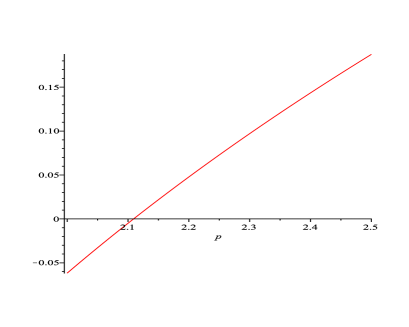
Figure 1. The graph of $m_{1}(p)-m_{0}(p)$ on $p\in[2,2.5]$.

In the second case we first find the interval with respect to $p$ where the inequality $m_{1}(p)\leq m_{0}(p)$ actually holds. Namely, it holds for

$$p\in[2,p_{*}],\quad p_{*}=2.10915\dots\,,$$

see Fig. 1, where the unique $p_{*}$ is found numerically.

Thus, inequality (3.1) holds for $p>p_{*}$ and we only need to look at the interval $p\in[2,p_{*}]$. Furthermore, since $m_{0}(p)$ in (3.5) is monotone increasing, we only need to check (3.1) for

$$p\in[2,p_{*}]\quad\text{and}\quad m\in[0,m_{*}],\ m_{*}=m_{0}(p_{*})=1.169\,\dots.$$

In view of (3.6), (3.7), (3.8) and the remark after (3.7) we have the following sequence of implications

$$\left\{I_{p}(m)<1\right\}\Leftarrow\left\{G(m,p)-1<0\right\}\Leftarrow\left\{A(z,p)\phi(z,p)<0\right\}\Leftrightarrow$$

$$\left\{\phi(z,p)<0\right\}\Leftarrow\left\{\phi(z_{*},p)<0\right\}\Leftrightarrow$$

$$\left\{6.1495p^{2}-30.8222p+13.7197<0,\ p\in[2,p_{*}]\right\}=\{^{\prime}\text{true}^{\prime}\},$$

where $z=m^{2}/2\leq z_{*}=m_{*}^{2}/2=0.6832<1$, and $m_{*}=1.169<\sqrt{2}$. Inequality (3.1) is now proved for the whole range of parameters and the proof is complete. ∎

Remark 3.1.

The case $p=2$ important for applications was treated by more elementary means in [7].

Remark 3.2.

Calculations show that for each $p$ tested, the function $I_{p}(m)$ is monotone increasing with respect to $m$. We are not able to prove it rigorously at the moment. However, it was shown in [8] that the lattice sum $J_{p}(m)$ in (1.5) is monotone increasing in $m$, which obviously implies inequality (1.5), since $J_{p}(\infty)=1$.

References

- [1] W. Beckner, Sharp Sobolev inequalities on the sphere and the Moser-Trudinger inequality. Ann. of Math. 138:2 (1993), 213–242.
- [2] M. F. Bidaut-Veron and L. Veron, Nonlinear elliptic equations on compact Riemannian manifolds and asymptotics of Emden equations. Invent. Math. 106 (1991), 489–539.
- [3] J. Dolbeault, M. J. Esteban, M. Kowalczyk, and M. Loss, Sharp interpolation inequalities on the sphere: new methods and consequences. Chin. Ann. Math. Ser. B 34:1 (2013), 99–112.
- [4] E. H. Lieb, An bound for the Riesz and Bessel potentials of orthonormal functions, J. Func. Anal. 51 (1983), 159–165.
- [5] A. A. Ilyin and S. V. Zelik, Sharp dimension estimates of the attractor of the damped 2D Euler-Bardina equations, In book: Partial Differential Equations, Spectral Theory, and Mathematical Physics, European Math. Soc. Press, Berlin, 2021, p. 209–229.
- [6] A. A. Ilyin, A. G. Kostianko, S. V. Zelik, Sharp upper and lower bounds of the attractor dimension for 3D damped Euler–Bardina equations. Physica D 432 (2022) 133156.
- [7] S. V. Zelik, A. A. Ilyin, and A. G. Kostianko, Dimension estimates for the attractor of the regularized damped Euler equations on the sphere. Mat. zametki 111:1 (2022), 55-67; English tansl. Math. Notes 111:1 (2022), 47–57.
- [8] A. A. Ilyin, A. G. Kostianko, and S. V. Zelik, Applications of the Lieb–Thirring and other bounds for orthonormal systems in mathematical hydrodynamics. arXiv:2202.01531.
- [9] K. I. Babenko, An inequality in the theory of Fourier integrals. Izv. Akad. Nauk SSSR 25 (1961), 531–542; English transl. Amer. Math. Soc. Transl. (2) 44 (1965), 115–128.
- [10] W. Beckner, Inequalities in Fourier analylis. Ann. of Math. 102 (1975), 159–182.
- [11] Sh. M. Nasibov, On optimal constants in some Sobolev inequalities and their application to a nonlinear Schrödinger equation, Dokl. Akad. Nauk SSSR. 307 (1989), 538–542; English transl. in Soviet Math. Dokl. 40 (1990).
- [12] E. Lieb, M. Loss, Analysis. Second edition. Graduate Studies in Mathematics, 14. American Mathematical Society, Providence, RI, 2001.
- [13] M. Weinstein, Nonlinear Schrödinger equations and sharp interpolation estimates. Comm. Math. Phys. 87 (1983), 567–576.
- [14] G. Talenti, Best constant in Sobolev inequality. Ann. di Matem. Pura ed Appl. 110 (1976), 353–372.
- [15] E. H. Lieb, Sharp constants in the Hardy–Littlewood–Sobolev and related inequalities. Annals of Math. 118 (1983), 349–374.
- [16] E. M. Stein and G. Weiss, Introduction to Fourier analysis on Euclidean spaces. Princeton University Press, Princeton NJ, 1972.
- [17] H. Araki, On an inequality of Lieb and Thirring. Lett. Math. Phys., 19:2 (1990), 167–170.
- [18] E. Lieb and W. Thirring, Inequalities for the moments of the eigenvalues of the Schrödinger Hamiltonian and their relation to Sobolev inequalities, Studies in Mathematical Physics, Essays in honor of Valentine Bargmann, Princeton University Press, Princeton NJ, 269–303 (1976).
- [19] B. Simon, Trace Ideals and Their Applications, 2nd ed. Amer. Math. Soc., Providence RI, 2005.
- [20] A. Ilyin, A. Laptev, and S. Zelik, Lieb–Thirring constant on the sphere and on the torus. J. Func. Anal. 279 (2020) 108784.
- [21] J. A. Hempel, G. R. Morris, and N. S. Trudinger, On the sharpness of a limiting case of the Sobolev imbedding theorem. Bull. Austral. Math. Soc. 3 (1970), 369–373.
- [22] A. A. Ilyin, Lieb–Thirring inequalities on the -sphere and in the plane, and some applications. Proc. London Math. Soc. 67 (1993), 159–182.
- [23] A. A. Ilyin, Partly dissipative semigroups generated by the Navier–Stokes system on two-dimensional manifolds and their attractors. Mat. Sbornik 184:1 (1993), 55–88; English transl. in Russ. Acad. Sci. Sb. Math. 78:1 47–76 (1993).
- [24] V. I. Krylov, Approximate calculation of integrals. Gos. Izdat. Fiz.–Mat. Lit., Moscow, 1959; English transl. Macmillan, New York, 1962.
- [25] S. V. Zelik, A. A. Ilyin, Green’s function asymptotics and sharp interpolation inequalities. Uspekhi Mat. Nauk 69:2 (2014), 23–76; English transl. in Russian Math. Surveys 69:2 (2014).