Hierarchical Bayesian Modelling for Knowledge Transfer Across Engineering Fleets via Multitask Learning

L.A. Bull lbull@turing.ac.uk D. Di Francesco M. Dhada O. Steinert T. Lindgren A.K. Parlikad A.B. Duncan M. Girolami The Alan Turing Institute, The British Library, London, NW1 2DB, UK Institute for Manufacturing, Department of Engineering, University of Cambridge, CB3 0FS, UK Strategic Product Planning and Advanced Analytics, Scania CV, Scania AB (publ), SE-151 87 Södertälje, Sweden Department of Computer and Systems Sciences, Stockholm University, P.O. Box 7003, SE-164 07 Kista, Sweden Department of Mathematics, Imperial College London, London, SW7 2AZ, UK Department of Engineering, University of Cambridge, CB3 0FA, UK

Abstract

A population-level analysis is proposed to address data sparsity when building predictive models for engineering infrastructure. Utilising an interpretable hierarchical Bayesian approach and operational fleet data, domain expertise is naturally encoded (and appropriately shared) between different sub-groups, representing (i) use-type, (ii) component, or (iii) operating condition. Specifically, domain expertise is exploited to constrain the model via assumptions (and prior distributions) allowing the methodology to automatically share information between similar assets, improving the survival analysis of a truck fleet and power prediction in a wind farm. In each asset management example, a set of correlated functions is learnt over the fleet, in a combined inference, to learn a population model. Parameter estimation is improved when sub-fleets share correlated information at different levels of the hierarchy. In turn, groups with incomplete data automatically borrow statistical strength from those that are data-rich. The statistical correlations enable knowledge transfer via Bayesian transfer learning, and the correlations can be inspected to inform which assets share information for which effect (i.e. parameter). Both case studies demonstrate the wide applicability to practical infrastructure monitoring, since the approach is naturally adapted between interpretable fleet models of different in situ examples.

keywords:

Hierarchical Bayesian Modelling; Multi-Task Learning; Asset Management; Transfer Learning

^†^†journal:

method		${\begin{array}[c]{@{}c@{}}k=2,\\ \;\;l=1\end{array}$}$	${\begin{array}[c]{@{}c@{}}k=3,\\ \;\;l=1\end{array}$}$	${\begin{array}[c]{@{}c@{}}k=2,\\ \;\;l=2\end{array}$}$	${\begin{array}[c]{@{}c@{}}k=3,\\ \;\;l=2\end{array}$}$	L
CP	-168	1555	4681	594	452	7114
CRL	52	1451	3359	282	-6	5138
STL	202	1619	5147	538	722	8229
MTL	218	1599	5206	549	686	8258

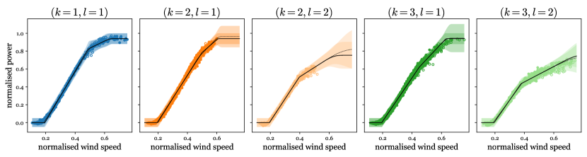
Refer to caption — Figure 17: Posteriorpredictivedistribution,themeanandthree-sigmadeviationfor:(lightshading,dashedline)Kindependentpower-curvemodelsp(y∗kl|xkl∗,xkl,ykl).(darkshading,solidline)multitasklearningwithmixedeffectsp(y∗kl|xkl∗,{{xkl,ykl}k=1Kl}l=1L).

Figure 18showstheposteriordistributionoftheparametersinferredattheindependentandfleetlevel.Thecut-inspeedqmovestowardsanaverageoftheindependentmodels,withreducedvariance;thisshouldbeexpectedsinceqbecomestiedasapopulationestimate.Thechangepointsqclusterintuitively,suchthatthenormalandcurtailedtasksformtwogroups(darkandlightshades).Theestimatedrparametersaresignificantlyimprovedthroughpartialpooling--inparticular,thegreenandorangedomainsshiftmuchfurtherfromtheweaklyinformativeprior.Thereisanotablereductioninthevarianceacrossalltasksfortheslopeestimatem2.Theaveragereductioninstandarddeviationacrosstheseparametersis25%.

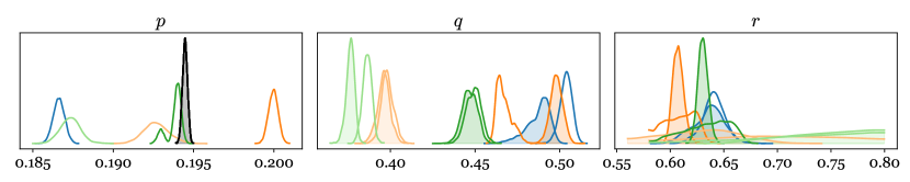
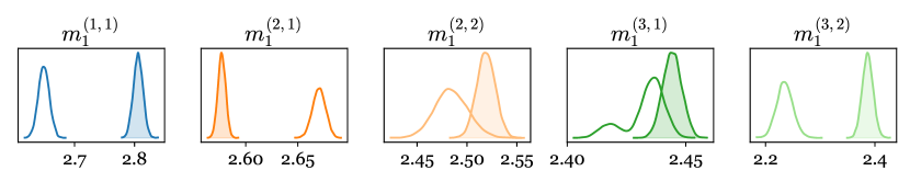
Figure 19presentsinsightsrelatingtomaximumpowerestimatesPm.ThetiedparameterforthenormalmaximumP(k,1)mmovestowardthedata-richestimate(blue)whilethecurtailedmaximumP(k,2)mmovestowardanaverageoftherelevanttasks(wherel=2).Inbothoperatingconditions,parametertyingenablesthemovefromvagueposteriorstodistributionswithclearexpectedvalues.Theaveragereductioninstandarddeviationforthenormalmaximumis82%,alongside37%forthecurtailedmaximum.

Finally,

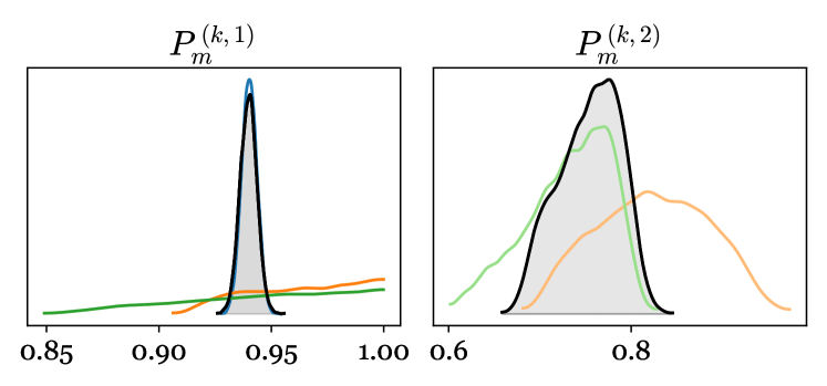
Figure 20plotsthePearsoncorrelationcoefficientofthepair-wiseconditionalsofqbetweentasks.(qispresentedsinceitisthemoststructured/insightful.)Itisclearthat,bymovingtoahierarchicalmodel,thecorrelationbetweenrelatedtasksisappropriatelycaptured,withtwodistinctblocksassociatedwiththenormalandcurtailedgroups.

6.4 Practicalimplications:Decisionanalysis

Inpractice,probabilisticpredictionsfromthepowermodelcanbeusedtosupportdecisionsatanylevelofthehierarchy,includingthepopulationlevel.Forexample,population-leveldecisionsareusefuliftheoperatordoesnotwishtocommittointeractingwithaspecificturbine.Consideradecisionproblem,wherebyanoperatormustcommittodeliveringaminimumpowerinsomeupcomingtimewindow.Thisinvolvesdecisionmakingunderuncertainty,andtheformal(statistical)proceduretoidentifytheexpectedoptimalactionrequiresaprobabilisticquantificationofwindspeedandpoweroutput.Thelattercanbeachievedbysamplingfromtheposteriorpredictivedistributionatthepopulationlevel,i.e.p(y∗∣x∗,θl),whereθl={P(l)m,m(l)1,p,q(l),r(l)}issampleddirectlyfromthegeneratingdistributions.Figure

21isanexampleofsuchapredictionforagivenwindspeed.

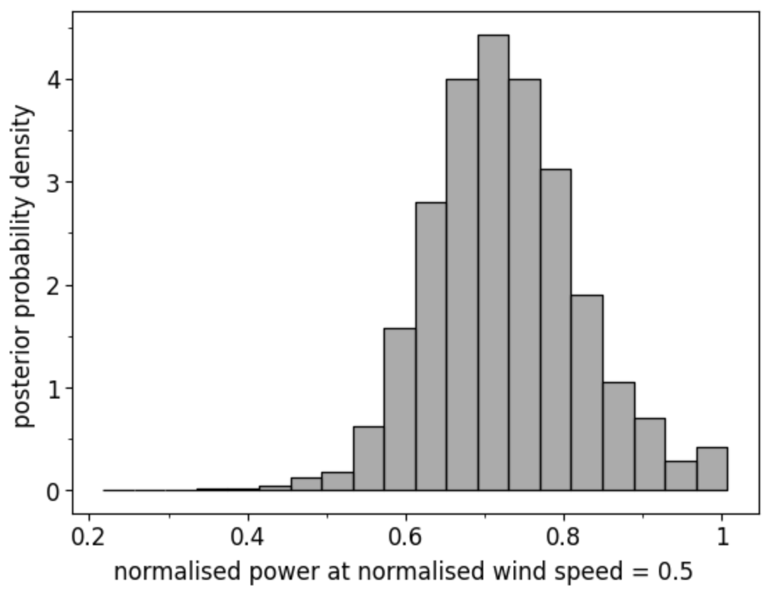
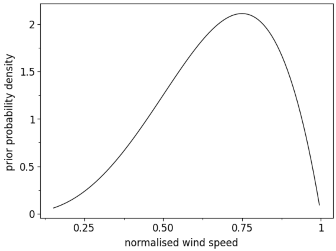
Predictionsatthislevelofthehierarchyareusefulsincetheyassumetheoperatorcannotcommittoaspecificturbine(atthisstage).Suchpredictionswouldnotbeavailablefromdomain-specific(independent)models;conversely,completepooling(ordomainadapted)predictionswouldnotformallyconsidertheadditionalvariabilityassociatedwithnon-specificturbineidentity.

Inthisexample,theoperatorhasthreeoptions,eachassociatedwithapayout(positiveutility)uponsuccessfullydeliveryofpowerandapenaltyfine(negativeutility)iftheturbinegeneratesinsufficientpower--thesevaluesarepresentedin

Table 4.Apriorprobabilisticmodelof(normalised)windspeedxprisshowninFigure22,asdescribedby,

\mathbf{x}_{pr}\sim\textrm{Beta}(4,2)

(32)

(Inpractice,thisinformationwouldlikelycomefromaforecastingmodel.)

Table 4: Financialoutcomesofdecisionanalysis.

Power Level	Payout	Penalty-fine
$L_{0}$ : 0.0	0.0	-0.0
$L_{1}$ : 0.5	0.3	-0.3
$L_{2}$ : 0.75	0.75	-1.0

Figure

LABEL:fig:prior_decision_treeshowsthedecision-eventtreerepresentationoftheproblem.Here,thesquare(decision)nodePLisassociatedwiththeavailablepowercommitmentsinTable4,suchthatPL={L0,L1,L2}.Thecircular(probabilistic)node(y∗∣xpr)istheprobabilisticpredictionofpower,giventhepriormodelofwindspeed.Finally,thetriangular(utility)nodeshowstheexpectedconsequenceofthedecision.

Foreachinstance,theexpectedoptimalactionPL∗∈{L0,L1,L2}