Robust measurements of n-point correlation functions of driven-dissipative quantum systems on a digital quantum computer

Abstract

We propose and demonstrate a unified hierarchical method to measure $n$-point correlation functions that can be applied to driven, dissipative, or otherwise non-equilibrium systems. In this method, the time evolution of the system is repeatedly interrupted by interacting an ancillary qubit with the system through a controlled operation, and measuring the ancilla immediately afterwards. We discuss robustness of this method versus ancilla-enabled interferometric techniques (such as the Hadamard test), and implement the method on a quantum computer in order to measure single-particle Green’s functions of a driven-dissipative fermionic system. This work shows that dynamical correlation functions for driven-dissipative systems can be measured with near-term quantum computers.

Introduction.— The characterization of quantum many-body systems still poses great theoretical challenges in a variety of disciplines. The calculation of dynamical correlation functions in particular is of the utmost importance, and reveals the spectral properties of complex models: In the case of the condensed matter models, the single-particle Green’s function takes into account how electrons propagate in the lattice, while two-particle Green’s functions (susceptibilities) contain information about the fluctuations of collective modes in the different physical channels (i.e. charge, spin, pairing), and three-point correlation functions describe how fermions interact with such collective modes. The evaluation of such quantities can get quite cumbersome, especially in the presence of strong correlation and when the entanglement increases rapidly during the system dynamics, as for example in the case of the two-dimensional Hubbard model that, despite the recent progress of numerical methods LeBlanc et al. (2015); Schäfer et al. (2021), still lacks a complete understanding. For this reason, quantum simulations Somma et al. (2002) represent a powerful resource for the computation of dynamical correlation functions of many-body systems.

Most protocols that have been put forward for the measurement of Green’s functions Wecker et al. (2015); Keen et al. (2020); Steckmann et al. (2021) are based on the Hadamard test Somma et al. (2002), where a controlled qubit is initialized in the $\left|+\right\rangle=\frac{1}{\sqrt{2}}(\left|0\right\rangle+\left|1\right\rangle)$ state via a Hadamard gate (H)Nielsen and Chuang (2010), and then entangled with the system qubits via a controlled unitary. Subsequently, after the system is evolved in time, another controlled unitary is applied. Finally, the information of the correlation function is extracted by performing measurements on the control qubit. This approach has been successfully used to obtain correlation functions and Green’s functions on quantum hardwareKreula et al. (2016a, b); Chiesa et al. (2019); Francis et al. (2020); Jaderberg et al. (2020); Sun et al. (2021); Steckmann et al. (2021). It has been shown that the same procedure can be used to extract quantum work statistics out of systems driven out of equilibrium Dorner et al. (2013) and for measuring OTOCs Swingle et al. (2016); Mi et al. .

While many studies were focused on extracting response functions of closed systems, less attention has been drawn on the evaluation of unequal-time correlation functions of open-quantum systems where the interaction between the system and a large environment can lead to quantitative and qualitative differences in the system dynamics. Lately, progress has been achieved in the construction of efficient quantum algorithms capable of addressing time-evolution of such dissipative-systems either exploiting the hardware intrinsic decoherence Tseng et al. (2000); Rost et al. (2020); Sommer et al. (2021), or by implementing Kraus maps and Lindblad operators Barreiro et al. (2011); Childs and Li (2017); Cleve and Wang (2016); Del Re et al. (2020); Tornow et al. (2020); Hu et al. (2020); Rost et al. (2021); Hu et al. (2021); Schlimgen et al. (2021); Kamakari et al. (2022), or non-Hermitian dynamics Hubisz et al. (2021); Zheng (2021), and this paves the way to the next step that would be the evaluation of dynamical correlation functions.

In this Letter, we first show that the Hadamard test methodology is still suitable to the case of a many-body driven-dissipative system. Such a protocol is advantageous because the measurement of a single qubit gives information about the correlation function of a many-body system with an arbitrary number of degrees of freedom. However, the coherent entanglement between the system and the ancilla must be preserved for the entire system dynamics, which is not normally possible without fault-tolerance. Hence, to overcome this problem, we propose a unified ancilla-based strategy to measure generic $n$-point correlation functions that does not require keeping the system and ancilla qubit in an entangled state. Our method is a single strategy capable of measuring arbitrary unequal-time correlation functions between multi-qubit Pauli operators, and which works for both dissipative and unitary time evolution. As such, it subsumes and unifies the approaches of Ref. Knap et al. (2013) (unequal-time commutators) and Ref. Uhrich et al. (2017) (unequal-time anticommutators). It is hierarchical in the sense that extracting the information of an $n$-th order correlation function requires previous knowledge of lower order correlation functions; but, it is robust, because it does not require system-ancilla entanglement to be maintained during the time evolution of the system. We verify the validity of our method by performing measurements of the single-particle Green’s function of a driven-dissipative fermionic model using a Quantinuum quantum computer. Our results show excellent quantitative agreement between data and the theoretical predictions.

Target quantities.— Our goal is the calculation of correlation functions of a generic system (S) that can also dissipate energy through an interaction with a bath (E); so we employ the density matrix formalism, which is required to study open quantum systems Breuer et al. (2002).

The correlation functions are constructed as follows. Let $\left\{O_{i}\right\}$ be a set of operators in the Schrödinger representation acting on the system Hilbert space with $i=1,2,\cdots n$, and let $\{t_{i}\}$ being a set of ordered time values such that $t_{0}<t_{1}<t_{2}<\ldots t_{n-1}<t_{n}$, where $t_{0}$ is the initial time, then we define the $n$-th rank correlation function via

$$\left<O_{n}(t_{n})O_{{n-1}}(t_{{n-1}})...O_{1}(t_{1})\right>$$

$$~{}~{}~{}~{}~{}=\mbox{Tr}_{\text{S}}\left\{O_{n}\mathcal{V}_{t_{n},t_{n-1}}...O_{2}\mathcal{V}_{t_{2},t_{1}}O_{1}\mathcal{V}_{t_{1},t_{0}}\rho(t_{0})\right\}.$$ (1)

Here, $O_{i}(t_{i})$ is the operator $O_{i}$ in the Heisenberg representation, $\rho(t_{0})$ is the system density matrix evaluated at the initial time, $\mathcal{V}_{t_{i+1},t_{i}}$ is the time evolution super-operator that evolves the system from time $t_{i}$ to $t_{i+1}$ (i.e. $\rho(t_{i+1})=\mathcal{V}_{t_{i+1,t_{i}}}\rho(t_{i})$ acting from left to right), and $\mbox{Tr}_{\text{S}}$ indicates a trace over the system subspace (meaning that the degrees of freedom of the bath have already been integrated out). For simplicity, and without loss of generality, we assume that the operators $O_{i}$ are unitary and Hermitian operators; addressing this case is sufficient to demonstrate the validity of our method, because a non-unitary operator can always be expanded as a linear combination of unitaries, chosen to also be Hermitian (e.g. Pauli strings). As will be shown in the next section, the correlation function in Eq. (Robust measurements of n-point correlation functions of driven-dissipative quantum systems on a digital quantum computer) can be extracted from the Hadamard test.

Instead, the alternative robust strategy that we propose will naturally yield correlation functions of nested commutators and anti-commutators of the form

$$\!\!\Big{\langle}[O_{1}(t_{1}),\!\big{[}O_{2}(t_{2}),\dots\,\!\big{[}O_{n-1}(t_{n-1}),O_{n}(t_{n})\big{]}_{\pm}\!\,\cdots\!\,\big{]}_{\pm}\big{]}_{\pm}\Big{\rangle},$$ (2)

where $[.\,,.]_{\pm}$ can be either commutators (-) or anti-commutators (+), all chosen independently. The quantity displayed in Eq. (Robust measurements of n-point correlation functions of driven-dissipative quantum systems on a digital quantum computer) could be obtained from the one in Eq. (2) and vice versa by performing multiple measurements and then combining the different outcomes together. The correlation function in Eq. (2) is not the most general $n$-point correlation function, because it always maintains Keldysh time ordering on a two branch Keldysh contour, as opposed to the most general form, which requires higher-order Keldysh contours Tsuji et al. (2017); for concrete examples, see the supplemental information sup . We note that in the case of two-point functions, Eq. (Robust measurements of n-point correlation functions of driven-dissipative quantum systems on a digital quantum computer) corresponds to lesser or greater Green’s functions while Eq. (2) to advanced, retarded, and Keldysh Green’s functions Stefanucci and van Leeuwen (2013), so both methods produce all the physical Green’s functions needed to describe a time evolving quantum system. In general, one cannot directly calculate out-of-time-ordered correlation functions with the circuit in Fig.(2) and we leave possible generalizations of this method to future work.

Hadamard test for driven-dissipative systems.—

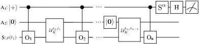
Figure 1: The standard interferometric scheme for measuring the $n$-time correlation function Somma et al. (2002), as given in Eq. (Robust measurements of n-point correlation functions of driven-dissipative quantum systems on a digital quantum computer), for a dissipative circuit. Accurate results require that the ancillary register $A_{1}$ maintain coherence over the entire duration of the circuit.

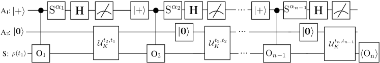
Figure 2: Circuit to measure a generic $n$-time correlation function of the kind defined in Eq.(2) using the robust strategy.

In Fig. 1, we show how the interferometry scheme proposed in Ref. Somma et al., 2002 generalizes to compute the $n$-time correlator defined in Eq. (Robust measurements of n-point correlation functions of driven-dissipative quantum systems on a digital quantum computer) for an open-quantum system. In order to simulate dissipative dynamics, we need a generic $k$-qubit ancilla register (called A₂) that we take to be initialized into the state $\left|\boldsymbol{0}\right\rangle=|0\rangle^{\otimes k}$. A suitable unitary operation $\mathcal{U}_{K}^{t,t^{\prime}}$ that entangles A₂ with the system register S followed by tracing out (ignoring) the state of the ancilla register can encode the time evolution map $\mathcal{V}_{t,t^{\prime}}$, which can be rewritten using the Kraus sum representation:

$$\mathcal{V}_{t,t^{\prime}}\,\rho(t^{\prime})=\sum_{i=0}^{2^{k}-1}K^{\,}_{i}(t,t^{\prime})\rho(t^{\prime})K^{\dagger}_{i}(t,t^{\prime}),$$ (3)

where $K_{i}$ are the so called Kraus operators satisfying the sum rule $\sum_{i}K^{\dagger}_{i}(t,t^{\prime})K^{\,}_{i}(t,t^{\prime})=\mathbbm{I}$. They are related to the unitary evolution of the system and ancilla bank as follows: $K_{i}(t,t^{\prime})=\left\langle i\right|\mathcal{U}_{K}^{t,t^{\prime}}\left|\boldsymbol{0}\right\rangle$, with $\{\left|i\right\rangle\}$ being a complete basis for A₂. In the interferometry scheme, we need an extra single-qubit ancilla register A₁ in which all the information about the correlation function (which is a complex number) will be stored. For example, in the case of $n=2$, the final quantum state of the A₁ qubit reads:

$$\rho_{A_{1}} =\left\{\begin{array}[]{c}\frac{1}{2}\hat{\mathbbm{I}}_{A_{1}}+\frac{1}{2}\text{Re}[C]\,\hat{\sigma}^{z}_{A_{1}}-\frac{1}{2}\text{Im}[C]\hat{\sigma}^{y}_{A_{1}}\,,\text{if }\alpha=0,\\ \\ \frac{1}{2}\hat{\mathbbm{I}}_{A_{1}}-\frac{1}{2}\text{Im}[C]\,\hat{\sigma}^{z}_{A_{1}}-\frac{1}{2}\text{Re}[C]\hat{\sigma}^{y}_{A_{1}}\,,\text{if }\alpha=1,\end{array}\right.$$ (7)

where $C=\left<O_{2}(t_{2})O_{1}(t_{1})\right>$. Measuring the ancilla in the $Z$ and $Y$ bases determines the real and imaginary parts of the correlation function.

This method is convenient because the complex information encoded in the correlation functions of a many-body system are found from single qubit measurements. However, this scheme requires maintaining the coherence of the A₁ ancilla (and thereby its entanglement with the system) for the full duration $t_{n}-t_{1}$. In the next section, we introduce an alternative robust scheme that does not require maintaining coherence of the $A_{1}$ ancilla, but at the cost of requiring a more complex measurement scheme.

Robust strategy.— In Fig. 2, we show the alternative circuit to measure the correlation function defined in Eq. (Robust measurements of n-point correlation functions of driven-dissipative quantum systems on a digital quantum computer). This circuit is schematic, because it encodes all possible circuits that are employed to measure the set of correlation functions in Eq. (2). Here, each realization has chosen unitary operations acting on A₁ (selected from $(S)^{\alpha_{i}}H$, where $S$ and $H$ are the phase gate and the Hadamard gate, respectively and $\alpha=\{0,1\}$ is a binary variable) for each time $t_{i}$ measured in the correlation function. It will turn out that the circuit shown in Fig. 2 naturally measures the set of correlation functions defined in Eq. (2) with the commutator or anti-commutator chosen from the $n-1$ dimensional binary vector $\boldsymbol{\alpha}=\{\alpha_{1},\alpha_{2},...,\alpha_{n-1}\}$. It is important to note that after the $S^{\alpha_{i}}H$ operation is performed, the ancilla qubit A₁ is measured immediately afterwards and the measurement outcome that we denote by $m_{i}$ is stored; such a measurement destroys the entanglement between A₁ and the state encoded in the system and the A₂ ancilla bank. The state is then evolved to the next $t_{i}$ using the Kraus map defined in Eq. (3). The $A_{1}$ ancilla is then reset to its $|+\rangle$ state and the process is repeated for each operator in the correlation function. In the last step, after the final time evolution from $t_{n-1}$ to $t_{n}$, the $S$ register qubits will be in a final state $\rho_{n}$ and the operator O_n is measured directly on the $S$ register qubits, yielding results that depend on $\boldsymbol{\alpha}$. The correlation function is determined by classical post-processing of the accumulated results and the choice of $\boldsymbol{\alpha}$.

In general, the state of the system qubits at time $t_{j+1}$ is obtained from the state at $t_{j}$ through the following map:

$$\rho_{j+1}\propto\mathcal{V}_{t_{j+1},t_{j}}\left(\rho_{j}+O_{j}\rho_{j}O_{j}+[(-1)^{m_{j}}i^{\alpha_{j}}O_{j}\rho_{j}+\text{h.c.}]\right),$$ (8)

where the proportionality constant is given by tracing the RHS of the equation. Here, $m_{j}=\{0,1\}$ is the result of the A₁ qubit measurement, and $\rho_{j=1}=\rho(t_{1})$ is given by the initial state of the system at time $t_{1}$ (see Fig. 2).

In order to show how this method works in practice, we discuss the two simplest cases: i.e. the two-point and the three-point correlation functions. For $n=2$, the result of measuring $O_{2}$ directly on the system register will yield

$$\text{Tr}\,O_{2}\,\rho_{2}=\mathcal{N}\left\{\left<O_{2}(t_{2})\right>+\left<O_{2}(t_{2})\right>_{O_{1}}\right.$$

$$+\left.{(-1)^{m_{1}}}\left[i^{\alpha_{1}}\left<O_{2}(t_{2})O_{1}(t_{1})\right>-i^{-\alpha_{1}}\left<O_{1}(t_{1})O_{2}(t_{2})\right>\right]\right\},$$

where $\mathcal{N}=\{2+\big{[}(-1)^{m_{1}}i^{\alpha_{1}}\left<O_{1}(t_{1})\right>+\text{h.c.}\big{]}\}^{-1}$, $\left<O_{1}(t_{1})O_{2}(t_{2})\right>=\text{Tr}\left(O_{2}\,\mathcal{V}_{t_{2},t_{1}}[\rho(t_{1})O_{1}]\right)$, and $\left<O_{2}(t_{2})\right>_{O_{1}}=\text{Tr}\left(O_{2}\,\mathcal{V}_{t_{2},t_{1}}[O_{1}\rho(t_{1})O_{1}]\right)$. Hence, when $\alpha_{1}=0,1$ the term in square brackets in Eq. (Robust measurements of n-point correlation functions of driven-dissipative quantum systems on a digital quantum computer) is proportional to $\left<[O_{1}(t_{1}),O_{2}(t_{2})]_{\mp}\right>$. This is precisely Eq. (2) when $n=2$.

For $n=3$, measuring $O_{3}^{\,}$ results in the following quantity:

$$\text{Tr}\,O_{3}\,\rho_{3}=(-1)^{m_{1}+m_{2}}\,C^{\boldsymbol{\alpha}}_{t_{1},t_{2},t_{3}}+R_{\boldsymbol{\alpha}},$$ (10)

where $C^{\boldsymbol{\alpha}}_{t_{1},t_{2},t_{3}}$ is a three-time correlation function that depends on the values of $\boldsymbol{\alpha}$. There are four possible values $\left<[O_{1}^{\,}(t_{1}),[O_{2}{\,}(t_{2}),O_{3}^{\,}(t_{3})]_{\pm}]_{\pm}\right>$. In addition, there are contributions denoted by $R_{\boldsymbol{\alpha}}$, which is a remainder function. It is determined by performing additional measurements comparable to what is needed for lower-rank correlation functions (see supplemental information for details: sup ).

We note that in the case of single-qubit Knap et al. (2013); Uhrich et al. (2017); Schuckert and Knap (2020) and two-qubit Mitarai and Fujii (2019) correlators, there are alternative ways of measuring correlation functions that do not require the extra ancillary register A₁.

Hardware implementation— In order to verify the validity of the protocol, we applied it to measure the Green’s function of spinless free fermions in a lattice driven by a constant electric field that also dissipate energy through a coupling with a thermal bath. The Hamiltonian of this chosen system plus bath can be brought into a block-diagonal form after performing a Fourier transform to momentum space as described in Ref. Del Re et al. (2020). Hence, the system’s reduced density matrix factorizes as a tensor product in momentum space, i.e., $\bigotimes_{k}\rho_{k}$ , and we can define a (diagonal in $k$) master equation for each 2$\times$ 2 $k$-dependent density matrix $\rho_{k}$,

$$\partial_{t}\rho_{k}=-i[\mathcal{H}_{k}(t),\rho_{k}]+\sum_{\ell=\{1,2\}}L_{\ell}^{\,}\,\rho_{k}\,L_{\ell}^{{\dagger}}-\{\rho_{k},L^{\dagger}_{\ell}L^{\,}_{\ell}\},$$ (11)

where the Lindblad operators are $L_{1}=\sqrt{\Gamma\,n_{F}(\epsilon_{k}(t))}d_{k}$ and $L_{2}=\sqrt{\Gamma\,n_{F}(-\epsilon_{k}(t))}d^{\dagger}_{k}$, with $d_{k}^{\,}$ being the destruction operator of a lattice fermion with quasi-momentum $k$, $\epsilon_{k}(t)=-2J\cos\left(k+\Omega\,t\right)$, with $J$ being the hopping amplitude, $\Omega$ the amplitude of the applied DC field, and $k$ the crystalline momentum. $\Gamma$ sets the strength of the system-environment coupling and $n_{F}(x)=\left[1+\exp(\beta\,x)\right]^{-1}$ is the Fermi-Dirac distribution with $\beta$ being the inverse of the bath temperature.

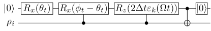
Figure 3: Circuit implementing the trotterised time evolution $\mathcal{U}_{K}(t,t+\Delta t)$ of the model defined in Eq. (11).

In Fig. 3, we show the circuit implementing $\mathcal{U}_{K}$ for the Kraus map related to Eq. (11). The Lindblad operator $L_{1(2)}$ encodes the physical process of a Bloch electron (hole) with momentum $k$ to hop from the lattice to the bath with a probability given by $\Gamma n_{F}[-\epsilon_{k}(t)]$ $(\Gamma n_{F}[\epsilon_{k}(t)])$. Such a decay process introduces a time dependence of the momentum distribution function of fermions and a damping of Bloch oscillations that eventually leads to a non-zero average of the DC-current sup ; Han (2013); Del Re et al. (2020); Rost et al. (2021).

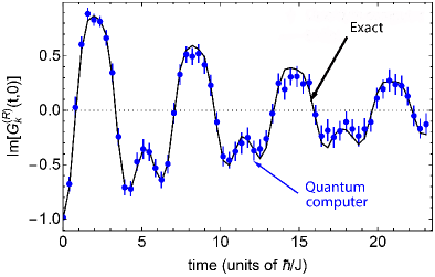
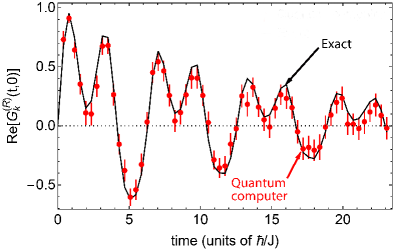
Figure 4: Imaginary (upper panel) and real (lower panel) parts of the retarded fermion Green’s function as a function of time (parameters are wavevector $ka=-0.5$, dimensionless electric field is $\Omega=1$, the dissipation rate to the fermionic bath is $\Gamma=1/16$ and the bath temperature is 0.01 in units of the hopping). Circles represent data from a Quantinuum model-H1 quantum computer, with error bars representing 2$\sigma$ confidence intervals. The primary source of error in the implemented circuits is due to noise on the two-qubit gates [$(2-3)\times 10^{-3}$ average infidelity]. However, the resulting noise model leads to results that are barely distinguishable by eye from exact circuit simulations (black lines) and are omitted from the figure.

In Fig. 4, we show the retarded fermion Green’s function $G_{k}^{(R)}(t,t^{\prime})=-i\theta(t-t^{\prime})\left<[d^{\,}_{k}(t),d^{{\dagger}}_{k}(t^{\prime})]_{+}\right>$ measured on Quantinuum’s model H1 quantum computer . The retarded Green’s function of the model can be computed exactly and its derivation and analytical form are given in the supplemental materials sup .

We notice an excellent quantitative agreement between the data produced by the quantum computer and the expected curves in presence of noise. It is worthwhile to note that in the presence of a driving field, the Green’s function does not oscillate as a simple sinusoidal function and it presents extra features, such as the additional maxima and minima occurring between time 10 and time 19 [see Fig. 4], that are faithfully reproduced by the quantum computer data.

Outlook.— We have put forward a robust technique for the measurement of multi-point correlation functions of driven-dissipative quantum systems that could be applied in the realm of quantum simulations of complex models such as the Hubbard model. We compared our strategy to the Ramsey interferometry scheme (generalized to the case of dissipative systems): while the latter requires us to keep the ancilla and system qubits in an entangled state for the entire time evolution of the system, the former does not. Such an advantage comes at the cost of performing extra measurements and also requires additional circuits of lower depth than the one needed to extract the target quantity. Furthermore, our method naturally computes correlators of the form given in Eq. (2). We applied our method to measuring the Green’s function of free fermions driven out of equilibrium and interacting with a bath. The data obtained from the quantum computer are in an excellent agreement with the curves predicted by the theory. While this data constitutes an important proof of principle enabling the measurement of correlation functions on near-term quantum computers, further work needs to be done to use this approach to solve new problems in science.

Interestingly, given its generality the Hadamard test has applications other than the measurement of correlation functions , for example it has been proposed for determining important overlaps in the realm of variational quantum dynamics simulations Yuan et al. (2019); Yao et al. (2021) and also for the simulation of open quantum systems using quantum imaginary-time evolution Kamakari et al. (2022). We therefore expect our robust alternative strategy to the Hadamard test to be suitable for these other applications as well.

Acknowledgments.— We acknowledge financial support from the U.S. Department of Energy, Office of Science, Basic Energy Sciences, Division of Materials Sciences and Engineering under Grant No. DE-SC0019469. BR was also funded by the National Science Foundation under Award No. DMR-1747426 (QISE-NET). JKF was also funded by the McDevitt bequest at Georgetown University.

Appendix A Correlation functions on the Keldysh contour

In this appendix, we discuss more in detail what kind of correlation functions can be evaluated by the circuit in Fig.(2) in the main text and what are those for which a generalization of our scheme is needed. In general, since the operators $O_{i}(t_{i})$ do not commute with each other, one can construct $n!$ correlation function out of all possible permutations of the operators in Eq.(Robust measurements of n-point correlation functions of driven-dissipative quantum systems on a digital quantum computer) in the main text. However calculating all possible nested commutators/anti-commutators of Eq.(2) gives the possibility of isolating only $2^{n-1}$ of these permutations.

Here we argue that the permutations we have access to correspond to components of time-ordered correlation functions on a simple two-branch Keldysh contour [see Fig.(5a) ], while the reaming ones are components of time-ordered correlation functions on a more complicated contour with multiple branches [see Fig.(5b)].

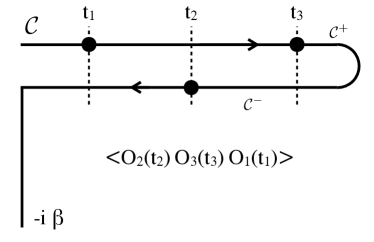
(a) (b)

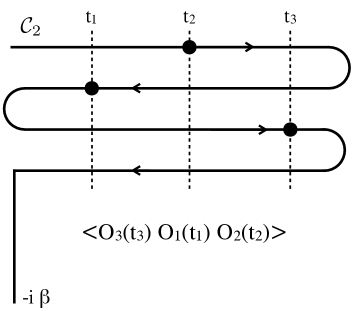
Figure 5: (a) Simple Keldysh contour $\mathcal{C}$ made up of the two forward ($\mathcal{C}^{+}$) and backward ($\mathcal{C}^{-}$) branches. Black dots specify on which branch the three different operators appearing in the permutation $\left<O_{2}O_{3}O_{1}\right>$ are evaluated. (b) Multiple-branch Keldysh contour $\mathcal{C}_{2}$ needed for the evaluation of the permutation $\left<O_{3}O_{1}O_{2}\right>$. In this case, one cannot evaluate $O_{3}$ on one of the first two branches and keep the product $O_{3}O_{1}O_{2}$ ordered on the contour at the same time. Time-ordering along the Keldysh contour, regardless of the number of branches (or whether time increases or decreases), simply proceeds by ordering along the arc length of the contour from start to finish.

Instead of giving a rigorous proof of our statement, we will consider the specific example for $n=3$. In this case, the permutations we have access to through Eq.(2) are: $\left<O_{1}(t_{1})O_{2}(t_{2})O_{3}(t_{3})\right>$, $\left<O_{1}(t_{1})O_{3}(t_{3})O_{2}(t_{2})\right>$, $\left<O_{2}(t_{2})O_{3}(t_{3})O_{1}(t_{1})\right>$ and $\left<O_{3}(t_{3})O_{2}(t_{2})O_{1}(t_{1})\right>$, where $t_{3}>t_{2}>t_{1}$. Hence, the following two permutations $\left<O_{3}(t_{3})O_{1}(t_{1})O_{2}(t_{2})\right>$ , $\left<O_{2}(t_{2})O_{1}(t_{1})O_{3}(t_{3})\right>$ are missing.

In Fig.(5a) we show a two-branch Keldysh contour Stefanucci and van Leeuwen (2013) $\mathcal{C}=\mathcal{C}_{+}+\mathcal{C}_{-}$, where $\mathcal{C}_{\pm}$ are the forward and backward branches. In the same figure we show that the particular permutation $\left<O_{2}O_{3}O_{1}\right>$ can be seen as a time-ordered function on the contour $\mathcal{C}$ where $t_{1}=t_{1+}$ and $t_{3}=t_{3+}$ lie on the forward branch while $t_{2}=t_{2-}$ lie on the backward branch.

Conversely, the permutation $\left<O_{3}O_{1}O_{2}\right>$ cannot be interpreted as a time-order correlation function on $\mathcal{C}$. Instead, it could be seen as a time-ordered correlation function on the more complex contour $\mathcal{C}_{2}$ shown in Fig.(5b) that contains two additional branches. The same contour has to be considered for the calculation of out-of-time correlators Tsuji et al. (2017), and therefore a generalization of our scheme is needed in order to have access to those quantities.

Appendix B Explicit calculations for the three-point correlation function

Here we shall derive Eq. (10) in the main text and give some insights about the remainder function and the additional measurements that are needed for its computation. In the derivation we shall use the following abstract notation for the time evolution: $\mathcal{V}_{t_{j+1},t_{j}}[\rho(t_{j})]=\rho(t_{j+1})$, instead of its sum representation in Eq. (3). We note that everything that is contained within the brackets of $\mathcal{V}$ is time-evolved as the density matrix in Eq. (3).

According to Eq. (8), the final state before the measurement in the system register in the case of $n=3$ reads:

$$\rho_{3} \propto \rho_{3}^{(\text{I})}+\rho_{3}^{(\text{II})}+\rho_{3}^{(\text{III})}+\left[\rho_{3}^{(\text{III})}\right]^{\dagger},$$ (12)

where:

$$\rho^{(\text{I})}_{3} = \mathcal{V}_{t_{3},t_{2}}[\rho_{2}]$$ (13)

$$\rho^{(\text{II})}_{3} = \mathcal{V}_{t_{3},t_{2}}[O_{2}\rho_{2}O_{2}]$$ (14)

$$\rho^{(\text{III})}_{3} = (-1)^{m_{2}}\,i^{\alpha_{2}}\mathcal{V}_{t_{3},t_{2}}[O_{2}\,\rho_{2}]$$ (15)

Because the time evolution preserves the trace, the normalization factor will be given by:

$$\mathcal{N}_{3}^{-1}=2+\left[(-1)^{m_{2}}\,i^{\alpha_{2}}\text{Tr}\left[\rho_{2}O_{2}\right]+\text{h.c.}\right].$$ (16)

There are a total of 16 terms on the RHS of Eq. (12): only four of them, those that are contained in $\rho^{(\text{III})}_{3}$ and its conjugate transpose, contain the information about the three-point correlation function. The other 12 terms give rise to the remainder function $R_{\boldsymbol{\alpha}}$ when $O_{3}$ is finally measured. As we shall see, these 12 spurious terms contain information about two-point and one-point (averages) correlation functions. Therefore, in order to extract the three-particle correlation function we will need to perform preliminary measurements of a few averages and two-point correlation functions that can be obtained using similar circuits as that one shown in Fig. 2 for $n=2$.

If we substitute $\rho_{2}$ from Eq. (10) into Eq. (13) we obtain:

$$\rho_{3}^{(\text{I})} = \rho(t_{3})+\mathcal{V}_{t_{3},t_{1}}[O_{1}\rho(t_{1})O_{1}]+$$ (17)

$$(-1)^{m_{1}} \,\mathcal{V}_{t_{3},t_{1}}\left[i^{\alpha_{1}}O_{1}\rho_{1}-i^{-\alpha_{1}}\rho_{1}O_{1}\right].$$

Analogously we obtain the explicit expression for Eq. (14), that reads:

$$\rho_{3}^{(\text{II})} = \mathcal{V}_{t_{3},t_{2}}[O_{2}\rho(t_{2})O_{2}]$$ (18)

$$+ \mathcal{V}_{t_{3},t_{2}}\left(O_{2}\mathcal{V}_{t_{2},t_{1}}[O_{1}\rho(t_{1})O_{1}]O_{2}\right)$$

$$+ (-1)^{m_{1}}\,i^{\alpha_{1}}\mathcal{V}_{t_{3},t_{2}}\left(O_{2}\mathcal{V}_{t_{2},t_{1}}[O_{1}\rho_{1}]O_{2}\right)$$

$$+ (-1)^{m_{1}}i^{-\alpha_{1}}\mathcal{V}_{t_{3},t_{2}}\left(O_{2}\mathcal{V}_{t_{2},t_{1}}[\rho_{1}O_{1}]O_{2}\right).$$

It is worthwhile to note that all the terms in Eqs. (17) and (18) contribute solely to the remainder function. For example, let us consider the following average that emerges from the last two terms in the RHS of Eq. (18), i.e. $i^{\alpha_{1}}\text{Tr}\,O_{3}\,\mathcal{V}_{t_{3},t_{2}}\left(O_{2}\mathcal{V}_{t_{2},t_{1}}[O_{1}\rho_{1}]O_{2}\right)+\text{h.c.}$: Such a quantity can be measured using the circuit shown in Fig. 6, that is very similar to the one displayed in Fig. 2 in the case of $n=2$, the only difference being the unitary operation $O_{2}$ that acts solely on the system qubits after the time evolution from $t_{1}$ to $t_{2}$ and the additional time evolution from $t_{2}$ to $t_{3}$.

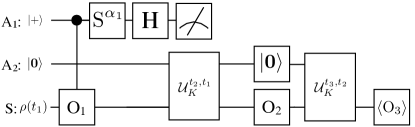
Figure 6: One of the preliminary measurements needed in order to compute the remainder function $R_{\boldsymbol{a}}$ in Eq. (10).

The explicit expressions of $\rho_{3}^{(\text{III})}$ reads:

$$\rho_{3}^{(\text{III})} = (-1)^{m_{2}}\,i^{\alpha_{2}}\mathcal{V}_{t_{3},t_{2}}[O_{2}\rho(t_{2})]$$

$$+ (-1)^{m_{2}}\,i^{\alpha_{2}}\mathcal{V}_{t_{3},t_{2}}\left(O_{2}\mathcal{V}_{t_{2},t_{1}}[O_{1}\rho(t_{1})O_{1}]\right)$$

$$+ (-1)^{m_{1}+m_{2}}i^{\alpha_{2}+\alpha_{1}}\mathcal{V}_{t_{3},t_{2}}\left(O_{2}\mathcal{V}_{t_{2},t_{1}}[O_{1}\rho(t_{1})]\right)$$

$$+ (-1)^{m_{1}+m_{2}}i^{\alpha_{2}-\alpha_{1}}\mathcal{V}_{t_{3},t_{1}}\left(O_{2}\mathcal{V}_{t_{2},t_{1}}[\rho(t_{1})O_{1}]\right).$$

We notice that the first two terms in the RHS of the last equation contribute to the remainder function. For example, the second term in the RHS of Eq. (B) would give rise to the following average $i^{\alpha_{2}}\,\text{Tr}\,O_{3}\mathcal{V}_{t_{3},t_{2}}\left(O_{2}\mathcal{V}_{t_{2},t_{1}}[O_{1}\rho(t_{1})O_{1}]\right)+\text{h.c.}$ that could be measure using the circuit displayed in Fig.7.

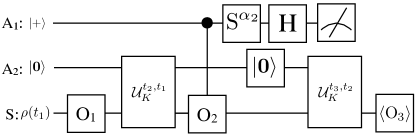
Figure 7: Quantum circuit needed in order to compute a contribution to the remainder function $R_{\boldsymbol{\alpha}}$ arising from $\rho^{(\text{III})}_{3}$ and its transpose conjugate [see Eq. (B) and the text beneath].

Therefore, by singling out the last two terms of Eq. (B), adding them up to their Hermitian conjugates, multiplying the results times $O_{3}$ and computing the trace, we obtain the following three-point correlation function:

$$C^{\boldsymbol{\alpha}}_{t_{1},t_{2},t_{3}} = i^{\alpha_{2}+\alpha_{1}}\overbrace{\text{Tr}\,O_{3}\,\mathcal{V}_{t_{3},t_{2}}\left(O_{2}\mathcal{V}_{t_{2},t_{1}}[O_{1}\rho(t_{1})]\right)}^{\left<\text{O}_{3}(t_{3})\text{O}_{2}(t_{2})\text{O}_{1}(t_{1})\right>}$$

$$+ i^{\alpha_{2}-\alpha_{1}}\overbrace{\text{Tr}\,O_{3}\,\mathcal{V}_{t_{3},t_{2}}\left(O_{2}\mathcal{V}_{t_{2},t_{1}}[\rho(t_{1})O_{1}]\right)}^{\left<\text{O}_{1}(t_{1})\text{O}_{3}(t_{3})\text{O}_{2}(t_{2})\right>}$$

$$+$$ h.c.

that is the one appearing in Eq. (10) in the main text.

The remainder function $R_{\boldsymbol{\alpha}}$ can be obtained in a similar way but adding up all the remaining 12 terms appearing in Eq. (12) multiplying them times $O_{3}$ and computing the trace. In order to extract the information about $C^{\boldsymbol{\alpha}}_{t_{1},t_{2},t_{3}}$, we will need to perform additional measurements similar to those shown in Figs. 6 and 7.

Appendix C Specifics of the model system implemented on the quantum computer

We model spinless electrons hopping on a one-dimensional lattice with nearest-neighbor hopping. The electrons are placed in an electric field and are connected to a fermionic bath that provides dissipation ton the system. See Refs. Del Re et al., 2020; Rost et al., 2021 for more details about the model and the derivation of Eq. (11).

C.1 Time evolution

The time evolution of such a model from time $t$ to $t+\Delta t$ is governed by the infinitesimal Kraus map that can be derived from the master equation in Eq. (11) and it is given by the following set of operators:

$$K_{0} =d^{\dagger}_{k}d^{\,}_{k}\sqrt{1-2\,\Gamma n_{F}[-\epsilon_{k}(t)]\Delta t}\,e^{-i\epsilon_{k}(t)\Delta t}$$

$$+d^{\,}_{k}d^{\dagger}_{k}\sqrt{1-2\Gamma n_{F}[\epsilon_{k}(t)]\Delta t},$$

$$K_{1} =\sqrt{2\Gamma\,\Delta t\,n_{F}[\epsilon_{k}(t)]}\,d^{\dagger}_{k},$$ (21)

$$K_{2} =\sqrt{2\Gamma\Delta t\,n_{F}[-\epsilon_{k}(t)]}d_{k}^{\,},$$

where $\epsilon_{k}(t)=-2J\cos\left(k+\Omega\,t\right)$, with $J$ being the hopping amplitude, $\Omega$ the amplitude of the applied DC field, and $k$ the crystalline momentum. $\Gamma$ measures the strength of the system-environment coupling and $n_{F}(x)=\left[1+\exp(\beta\,x)\right]^{-1}$ is the Fermi-Dirac distribution with $\beta$ being the inverse of the bath temperature. The Kraus map in Eq. (C.1) can be implemented on the system qubit using an extra-ancilla qubit as shown in the circuit in Fig.(3).

C.2 Calculation of the Green’s function

The Kraus map shown in Eq. (C.1) gives the time evolution from time $t$ to time $t+\Delta t$ and it is exact in the limit of $\Delta t\to 0^{+}$, for this reason we refer to it as an infinitesimal map. In order to write down the Green’s function analytically it is useful to derive the integrated map $V_{t,t^{\prime}}$ that gives the time evolution from time $t$ to $t^{\prime}>t$ with $t^{\prime}-t$ being a positive finite arbitrary number. This is equivalent to determining the Choi matrix, that Andersson et al. (2007); Del Re et al. (2020) reads: $S_{ab}(t)=\sum_{r_{0}}^{3}\sum_{s=0}^{3}F_{sr}(t)\text{Tr}[\sigma_{r}\sigma_{a}\sigma_{s}\sigma_{b}],$ where the indices $a,b$ specify one of the four operators $\sigma_{0}=\mathbbm{1}_{2\times 2}/\sqrt{2}$, $\sigma_{1}=\sigma^{x}/\sqrt{2}$, $\sigma_{2}=\sigma^{y}/\sqrt{2}$, $\sigma_{3}=\sigma^{z}/\sqrt{2}$. We can obtain a differential equation for the $F_{rs}(t)$ matrix by realizing that the master equation in Eq. (11) can be written as $\partial_{t}\rho=\Lambda_{t}(\rho)$, with $\Lambda_{t}$ being a linear map such that $\Lambda_{t}(\rho)$ is Hermitian and traceless. The equation of motion for $F$ reads: $\dot{F}=L(t)\cdot F(t)$, where the center dot indicates the matrix product, with initial condition $F(0)=\mathbbm{1}_{4\times 4}$ and with $L_{rs}=\text{Tr}[\sigma_{r}\Lambda_{t}(\sigma_{s})]$ . Once the Choi matrix is obtained we can write the time-evolution map in the Kraus represenation with Kraus operators: $K_{i}=\sqrt{\lambda_{i}}\sum_{a=0}^{3}X(i)_{a}\sigma_{a}$, where $\lambda_{i}$ and $X(i)$ are resepctively the eigenvalues and eigenvectors of S. In this way we obtain the following Kraus map:

$$K_{1} = A_{1}(k,t,t^{\prime})P_{0}+B_{1}(k,t,t^{\prime})P_{1},$$

$$K_{2} = A_{2}(k,t,t^{\prime})P_{0}+B_{2}(k,t,t^{\prime})P_{1},$$

$$K_{3} = \alpha(k,t,t^{\prime})X\,P_{0},$$

$$K_{4} = \beta(k,t,t^{\prime})X\,P_{1},$$ (22)

where $P_{0}=d^{\,}_{k}d^{\dagger}_{k}$, $P_{1}=d^{\dagger}_{k}d^{\,}_{k}$, $X=\frac{1}{\sqrt{2}}(d^{\,}_{k}+d^{{\dagger}}_{k})$ and we have:

$$A_{1} = \frac{\left(b-\sqrt{b^{2}+c^{2}+d^{2}}+c+id\right)\sqrt{a-\sqrt{b^{2}+c^{2}+d^{2}}}}{2(c+id)\sqrt{\frac{1}{\frac{b}{\sqrt{b^{2}+c^{2}+d^{2}}}+1}}}$$

$$B_{1} = -\frac{\left(\sqrt{b^{2}+c^{2}+d^{2}}-b+c+id\right)\sqrt{a-\sqrt{b^{2}+c^{2}+d^{2}}}}{2(c+id)\sqrt{\frac{1}{\frac{b}{\sqrt{b^{2}+c^{2}+d^{2}}}+1}}}$$

$$A_{2} = \frac{\left(\sqrt{b^{2}+c^{2}+d^{2}}+b+c+id\right)\sqrt{a+\sqrt{b^{2}+c^{2}+d^{2}}}}{2(c+id)\sqrt{\frac{1}{1-\frac{b}{\sqrt{b^{2}+c^{2}+\text{d}^{2}}}}}}$$

$$B_{2} = \frac{\left(\sqrt{b^{2}+c^{2}+d^{2}}+b-c-id\right)\sqrt{a+\sqrt{b^{2}+c^{2}+d^{2}}}}{2(c+id)\sqrt{\frac{1}{1-\frac{b}{\sqrt{b^{2}+c^{2}+d^{2}}}}}}$$

and $a=\frac{1}{2}[1+e^{-2\Gamma(t-t^{\prime})}]$, $b=\cos[f_{k}(t,t^{\prime})]e^{-\Gamma(t-t^{\prime})}$, $c=\frac{1}{2}-n_{k}(t^{\prime})+e^{-\Gamma(t-t^{\prime})}(n_{k}(t^{\prime})-\frac{1}{2})$ with $n_{k}(t)=\text{Tr}[\rho_{k}(t)P_{1}]$, $d=e^{-\Gamma(t-t^{\prime})}\sin[f_{k}(t,t^{\prime})]$, $\alpha=\sqrt{c-\frac{1}{2}(1-e^{-2\Gamma(t-t^{\prime})})}$, $\beta=\sqrt{c+\frac{1}{2}(1-e^{-2\Gamma(t-t^{\prime})})}$.

The retarded Green’s function can be expressed in terms of the lesser and greater Green’s functions in the following way: $G^{(R)}_{k}(t,t^{\prime})=\theta(t-t^{\prime})\left[G^{>}_{k}(t,t^{\prime})-G^{<}_{k}(t,t^{\prime})\right]$, where $G_{k}^{>}(t,t^{\prime})=-i\left<d_{k}^{\,}(t)d^{{\dagger}}_{k}(t^{\prime})\right>=-i\,\text{Tr}\left\{X\,P_{1}\,V_{t,t^{\prime}}[X\,P_{0}\rho_{k}(t^{\prime})]\right\}$ and $G_{k}^{<}(t,t^{\prime})=i\left<d_{k}^{{\dagger}}(t^{\prime})d^{\,}_{k}(t)\right>=i\,\text{Tr}\left\{X\,P_{1}\,V_{t,t^{\prime}}\left[\rho_{k}(t^{\prime})X\,P_{0}\right]\right\}$.

A generic one-qubit density matrix can be written in the following way: $\rho(t)=\rho_{\text{diag}}+x(t)X+y(t)Y$, where $\rho_{\text{diag}}(t)=\text{diag}(1-n_{k}(t),n_{k}(t))$. It is easy to show that the lesser or greater Green’s function does not depend on the off-diagonal elements of the density matrix. In fact:

$$\text{Tr}\{XP_{1}V_{t,t^{\prime}}[(x\,X+y\,Y)XP_{0}]\}=$$

$$(x-i\,y)\,\text{Tr}\{XP_{1}V_{t,t^{\prime}}[P_{0}]\}=$$

$$(x-i\,y)\text{Tr}\{XP_{1}[(|A|_{1}^{2}+|A_{2}|^{2})P_{0}+|\alpha|^{2}P_{1}]\}=$$

$$(x-i\,y)|\alpha|^{2}\,\text{Tr}\{XP_{1}\}=0\,.$$

Therefore, we can write the lesser Green’s function as:

$$G^{<}_{k}(t,t^{\prime}) = i\text{Tr}\left\{V_{t,t^{\prime}}[\rho_{\text{diag}}XP_{0}]XP_{1}\right\}$$ (24)

$$= i\,n_{k}(t^{\prime})\,\text{Tr}\left\{V_{t,t^{\prime}}[P_{1}\,X\,P_{0}]XP_{1}\right\},$$

and by noticing that:

$$V_{t,t^{\prime}}[P_{1}\,X\,P_{0}] = K_{1}^{\,}\,P_{1}XP_{0}K_{1}^{\dagger}+K_{2}^{\,}P_{1}\,X\,P_{0}K_{2}^{\dagger}$$ (25)

$$= P_{1}\,X\,P_{0}\left(A_{1}^{*}B_{1}+A_{2}^{*}B_{2}\right),$$

we obtain:

$$G^{<}_{k}(t,t^{\prime}) = i\,n_{k}(t^{\prime})\left(A_{1}^{*}B_{1}+A_{2}^{*}B_{2}\right)\mbox{Tr}\left\{XP_{1}\,P_{1}XP_{0}\right\}$$ (26)

$$= i\,n_{k}(t^{\prime})\,e^{-\Gamma(t-t^{\prime})}e^{-if_{k}(t,t^{\prime})}$$

Analogously we obtain the following expression for the greater Green’s function:

$$G^{>}_{k}(t,t^{\prime}) = -i\text{Tr}\left\{X\,P_{1}\,V_{t,t^{\prime}}\left[XP_{0}\,\rho_{\text{diag}}\right]\right\}$$ (27)

$$= -i(1-n_{k}(t^{\prime}))e^{-\Gamma(t-t^{\prime})}e^{-if_{k}(t,t^{\prime})}.$$

Let us notice that only two Kraus operators, namely $K_{1}$ and $K_{2}$ were involved in the time evolution of the operator $\rho\,d_{k}^{\,}$ ($d^{\dagger}_{k}\,\rho$) in the expression of the lesser (greater) Green’s function. From Eqs. (26) and (27), we obtain the retarted Green’s function as following:

$$G^{(R)}_{k}(t,t^{\prime}) = \theta(t-t^{\prime})[G_{k}^{>}(t,t^{\prime})-G_{k}^{<}(t,t^{\prime})]$$ (28)

$$= -i\theta(t-t^{\prime})\,e^{-\Gamma(t-t^{\prime})}e^{-if_{k}(t,t^{\prime})}.$$

References

LeBlanc et al. (2015)J. P. F. LeBlanc, A. E. Antipov, F. Becca, I. W. Bulik,
G. K.-L. Chan, C.-M. Chung, Y. Deng, M. Ferrero, T. M. Henderson, C. A. Jiménez-Hoyos, E. Kozik, X.-W. Liu, A. J. Millis, N. V. Prokof’ev, M. Qin,
G. E. Scuseria, H. Shi, B. V. Svistunov, L. F. Tocchio, I. S. Tupitsyn, S. R. White, S. Zhang, B.-X. Zheng, Z. Zhu, and E. Gull (Simons Collaboration on
the Many-Electron Problem), Phys. Rev. X 5, 041041 (2015).
Schäfer et al. (2021)T. Schäfer, N. Wentzell,
F. Šimkovic, Y.-Y. He, C. Hille, M. Klett, C. J. Eckhardt, B. Arzhang, V. Harkov, F. m. c.-M. Le Régent, A. Kirsch, Y. Wang, A. J. Kim, E. Kozik, E. A. Stepanov,
A. Kauch, S. Andergassen, P. Hansmann, D. Rohe, Y. M. Vilk, J. P. F. LeBlanc, S. Zhang, A.-M. S. Tremblay, M. Ferrero,
O. Parcollet, and A. Georges, Phys. Rev. X 11, 011058 (2021).
Barreiro et al. (2011)J. T. Barreiro, M. Müller, P. Schindler, D. Nigg,
T. Monz, M. Chwalla, M. Hennrich, C. F. Roos, P. Zoller, and R. Blatt, Nature 470, 486 (2011).
Note (1)Short-time data (prior to ) was taken on the Honeywell
model H0 quantum computer, while later time data were obtained on an updated
Quantinuum model H1 computer.
Yuan et al. (2019)X. Yuan, S. Endo, Q. Zhao, Y. Li, and S. C. Benjamin, Quantum 3, 191
(2019).
Yao et al. (2021)Y.-X. Yao, N. Gomes, F. Zhang, C.-Z. Wang, K.-M. Ho, T. Iadecola, and P. P. Orth, PRX Quantum 2, 030307 (2021).