Origin of primeval seed magnetism in rotating astrophysical bodies

Abstract

We show that a primeval seed magnetic field arises due to spin-degeneracy breaking of fermions caused by the dragging of inertial frames in the curved spacetime of rotating astrophysical bodies. This seed magnetic field would arise even due to electrically neutral fermions such as neutrons. As an example, we show that an ideal neutron star rotating at $500$ revolutions per second, having mass $0.83$ M_⊙ and described by an ensemble of degenerate neutrons, would have $0.12$ Gauss seed magnetic field at its center arising through the breaking of spin-degeneracy.

I Introduction

Magnetic fields are observed in the universe on widely different scales. Its field strengths are seen to vary from being as small as $10^{-16}$ Gauss in the voids of intergalactic medium Neronov and Vovk (2010); Essey et al. (2011); Dolag et al. (2010); Takahashi et al. (2013), around $10^{-6}$ Gauss within a galaxy and in the range of $10^{8}-10^{15}$ Gauss in a rotating neutron star Tiengo et al. (2013). Given a small seed magnetic field, there exists mechanism such as the turbulent dynamo Zhang et al. (2009); Bucciantini and Del Zanna (2013) that can rapidly amplify the magnetic field strength in astrophysical systems. However, a seemingly innocuous yet profound question remains poorly understood — what is the origin of the seed magnetism itself? At present there exist largely two different types of model for the seed magnetism where the seed field is viewed either as a cosmic relic of the early universe physics or as being generated by ionized plasma through the astrophysical processes Cho (2014); Ichiki et al. (2006); Doi and Susa (2011). However, these models come with their own set of shortcomings such as present field strength being incompatible with early universe physics or having insufficient sustenance and coherence of the seed field (see Subramanian (2019); Brandenburg and Subramanian (2005) for an excellent review).

In this article, we show that a natural answer to the question of seed magnetism arises from two fundamental theories of nature, namely Einstein’s general theory of relativity and Dirac’s theory of fermions when they are put together. This answer does not require any new exotic physics but a proper reconciliation of the Dirac theory together with the general relativity through the methods of quantum field theory in the curved spacetime. In particular, we show that the genesis of seed magnetism is a direct consequence of spin-degeneracy breaking of fermions caused by the curved spacetime of rotating astrophysical bodies, principally due to the dragging of inertial frames. This seed magnetism would arise even due to electrically neutral fermions such as neutrons.

II Fermions in curved spacetime

In Fock-Weyl formulation, dynamics of a free Dirac fermion $\psi$ in a generally curved spacetime is described by an invariant action

$$S_{\psi}=-\int d^{4}x\sqrt{-g}~{}\bar{\psi}[i\gamma^{a}{e^{\mu}}_{a}\mathcal{D}_{\mu}+m]\psi~{},$$ (1)

where Dirac adjoint $\bar{\psi}=\psi^{\dagger}\gamma^{0}$ and $m$ is the mass of the fermion. Here ${e^{\mu}}_{a}$ are the tetrad components defined in terms of the global metric $g_{\mu\nu}$ as $g_{\mu\nu}{e^{\mu}}_{a}{e^{\nu}}_{b}=\eta_{ab}$ where $\eta_{ab}=diag(-1,1,1,1)$ is the Minkowski metric. Spin-covariant derivative for the fermion field $\psi$ is defined as $\mathcal{D}_{\mu}\psi\equiv\partial_{\mu}\psi+\Gamma_{\mu}\psi$ together with the spin connection

$$\Gamma_{\mu}=-\tfrac{1}{8}\eta_{ac}{e_{\nu}}^{c}(\partial_{\mu}{e^{\nu}}_{b}+\Gamma^{\nu}_{\mu\sigma}{e^{\sigma}}_{b})~{}[\gamma^{a},\gamma^{b}]~{},$$ (2)

where $\Gamma^{\nu}_{\mu\beta}$ are the Christoffel connections and $\gamma^{a}$ are the Dirac matrices in Minkowski spacetime, satisfying the Clifford algebra $\{\gamma^{a},\gamma^{b}\}=-2\eta^{ab}\mathbb{I}$. The minus sign in front of the metric $\eta^{ab}$ here ensures that usual relations $(\gamma^{0})^{2}=\mathbb{I}$ and $(\gamma^{k})^{2}=-\mathbb{I}$ for $k=1,2,3$ holds true for the chosen metric signature. The Lagrangian density $\mathcal{L}$ corresponding to the action (1) is expressed as $S_{\psi}=\int d^{4}x\sqrt{-g}~{}\mathcal{L}~{}$.

III Axially symmetric stationary spacetime

In order to describe the spacetime around a rotating astrophysical body, we consider its matter distribution to be axially symmetric and stationary. In natural units $c=\hbar=1$, the metric due to an axially symmetric, stationary and slowly rotating matter distribution can be expressed as Hartle (1967)

$$ds^{2}=-H^{2}dt^{2}+Q^{2}dr^{2}+r^{2}K^{2}[d\theta^{2}+\sin^{2}\theta(d\varphi-Ldt)^{2}]~{},$$ (3)

where metric functions $H$, $Q$, $K$ and $L$ depend only on the coordinates $r$ and $\theta$. Here we require these functions to be such that the metric (3) is asymptotically flat. The function $L$ represents acquired angular velocity of a freely-falling observer from infinity, a phenomena known as the dragging of inertial frames. For most rotating astrophysical bodies the frame-dragging angular velocity is small such that $(rL)\ll 1$. So for simplicity we shall ignore terms which are $\mathcal{O}(L^{2})$. These metric functions are governed by Einstein’s equation $G_{\mu\nu}=8\pi GT_{\mu\nu}$. We represent the matter distribution here by a perfect fluid with the stress-energy tensor

$$T_{\mu\nu}=(\rho+P)u_{\mu}u_{\nu}+Pg_{\mu\nu}~{},$$ (4)

where $u^{\mu}$ is the 4-velocity of the fluid, $P$ is its pressure and $\rho$ is its energy density.

IV Reduced action

In the Einstein equation, the pressure and the energy density are considered to be varying functions of the coordinates in general. However, in equilibrium statistical mechanics, these thermodynamical quantities are considered to be uniform within a given system. These two seemingly disparate aspects therefore need to be combined consistently by using the notion of local thermodynamical equilibrium. In essence, one has to consider two distinct scales — the astrophysical scale over which Einstein’s equation operates and the scale of microscopic physics over which local thermodynamical equilibrium is achieved. In order to ensure a local thermodynamical equilibrium, here we consider a small region around every spatial point such that the variation of the metric functions within the region can be neglected. The small region nevertheless, must contain sufficiently large number of degrees of freedom to ensure a thermal equilibrium. The later condition, in the context of quantum statistical physics, requires wave functions representing those degrees of freedom should be sufficiently localized.

For definiteness, let us consider a small spatial box whose center is located at the coordinates $(r_{0},\theta_{0})$. By defining a new set of local coordinates as $X=Q_{0}r\sin\bar{\theta}\cos\bar{\varphi}$, $Y=Q_{0}r\sin\bar{\theta}\sin\bar{\varphi}$, and $Z=Q_{0}r\cos\bar{\theta}$ where $\bar{\theta}=\xi_{1}\theta$, $\bar{\varphi}=\xi_{0}\varphi$ with $\xi_{1}=(K_{0}/Q_{0})$, $\xi_{0}=(\xi_{1}\sin\theta_{0})/\sin(\xi_{1}\theta_{0})$, the metric (3) can be reduced within the box to be

$$g_{\mu\nu}=\begin{bmatrix}-\mathcal{N}^{2}&\omega Y&-\omega X&0\\ \omega Y&1&0&0\\ -\omega X&0&1&0\\ 0&0&0&1\end{bmatrix}~{},$$ (5)

where $\omega=\xi_{0}L_{0}$ and $\mathcal{N}^{2}=H^{2}_{0}$. Here we have assumed that the metric functions take a fixed set of values $H_{0}$, $Q_{0}$, $K_{0}$ and $L_{0}$ within the box such that $Q_{0}\geq K_{0}$ i.e. $\xi_{1}\leq 1$. Additionally, we have approximated $\sin^{2}\theta d\varphi=\sin^{2}(\theta_{0}+\delta\theta)d\varphi\approx\sin^{2}\theta_{0}d\varphi$ for all points within the box.

The non-vanishing tetrad components corresponding to the metric (5), can be expressed as ${e^{X}}_{1}={e^{Y}}_{2}={e^{Z}}_{3}=1$, ${e^{t}}_{0}=\mathcal{N}^{-1}$, ${e^{X}}_{0}=-\omega Y\mathcal{N}^{-1}$, ${e^{Y}}_{0}=\omega X\mathcal{N}^{-1}$ whereas non-vanishing components of the inverse tetrad ${e_{\mu}}^{a}$ can be written as ${e_{X}}^{1}={e_{Y}}^{2}={e_{Z}}^{3}=1$, ${e_{t}}^{0}=\mathcal{N}$, ${e_{t}}^{1}=\omega Y$, ${e_{t}}^{2}=-\omega X$. Non-vanishing components of the Christoffel connection are given by $\Gamma^{X}_{tY}=\Gamma^{X}_{Yt}=-\Gamma^{Y}_{tX}=-\Gamma^{Y}_{Xt}=\omega$. Consequently, only non-vanishing component of the spin-connection $\Gamma_{\mu}$ is

$$\Gamma_{t}=-\frac{\omega}{4}[\gamma^{1},\gamma^{2}]=\frac{i\omega}{2}\Sigma_{3}~{},$$ (6)

where $\Sigma_{3}=\sigma^{3}\otimes\mathbb{I}_{2}$ with $\sigma^{3}$ being the third Pauli matrix. Therefore, the Dirac action (1) within the box reduces to

$$S_{\psi}=-\int d^{4}x~{}\bar{\psi}[i\gamma^{0}\partial_{t}+\mathcal{N}(i\gamma^{k}\partial_{k}+m)-\omega\gamma^{0}\hat{J}_{Z}]\psi~{},$$ (7)

where $\hat{J}_{Z}=(\hat{L}_{Z}+\tfrac{1}{2}\Sigma_{3})$ with $\hat{L}_{Z}=-i(X\partial_{Y}-Y\partial_{X})$. We note that $\hat{J}_{Z}$ can be naturally interpreted as the total angular momentum operator associated with the dragging of inertial frames where $\hat{L}_{Z}$ is the orbital angular momentum operator and $\sigma^{3}$ is the third Pauli matrix which is the spin operator along $Z$-direction. One may arrive at the reduced action (7) also by considering the transformation of the spinor field $\psi(x)\mapsto e^{i\hat{J}_{Z}\omega t}\psi(x)$ under a rotation around $Z$ axis with angular velocity $\omega$, starting from a non-rotating configuration.

V Partition function

We consider an ensemble of fermions in the box which is in a local thermodynamical equilibrium. Here we define the scale of temperature $T$ in the frame of an asymptotic observer where $\mathcal{N}\to 1$ and $\omega\to 0$. This choice allows us to treat the reduced action (7) as an effective action written in the Minkowski spacetime. It leads to a simpler computation as well as it helps to avoid the issues related to Wick rotation in a general curved spacetime Visser (2017). The effective action nevertheless includes the effects of curved spacetime through the fixed parameters $\mathcal{N}$ and $\omega$ in the given box. In order to compute the partition function, here we follow similar methods as used by the authors for computing equation of states in the curved spacetime of spherical stars Hossain and Mandal (2021a, b). Using coherent states of the Grassmann fields Laine and Vuorinen (2016); Das (1997); Kapusta and Landshoff (1989), the partition function corresponding to the action (7) can be expressed as $\mathcal{Z}_{\psi}=\int\mathcal{D}\bar{\psi}\mathcal{D}\psi\ e^{-S_{\psi}^{\beta}}$ where $S_{\psi}^{\beta}=\int_{0}^{\beta}d\tau\int d^{3}x(\mathcal{L}^{E}-\mu\bar{\psi}\gamma^{0}\psi)$. Here $\mu$ is the chemical potential of the fermion and $\beta=1/k_{B}T$ with $k_{B}$ being the Boltzmann constant. The Euclidean Lagrangian density is obtained through a Wick rotation as $\mathcal{L}^{E}=-\mathcal{L}(t\rightarrow-i\tau)$.

In a thermal equilibrium, the fermion field $\psi$ is subjected to the anti-periodic boundary condition $\psi(\tau,\mathbf{x})=-\psi(\tau+\beta,\mathbf{x})$. Consequently, in Fourier domain the Dirac field $\psi$ can be written as

$$\psi(\tau,\mathbf{x})=\frac{1}{\sqrt{V}}\sum_{l,\mathrm{k}}~{}e^{-i(\omega_{l}\tau+\mathrm{k}\cdot\mathbf{x})}\tilde{\psi}(l,\mathrm{k})~{},$$ (8)

where Matsubara frequencies are $\omega_{l}=(2l+1)\pi~{}\beta^{-1}$ with $l$ being an integer and $V=\int d^{3}x\sqrt{-\eta}$ is the volume of the box. Using the reduced action (7) it is convenient to express the partition function as $\ln\mathcal{Z}_{\psi}=\ln\mathcal{Z}_{0}+\ln\mathcal{Z}_{L}$ where $\mathcal{Z}_{0}=\int\mathcal{D}\bar{\psi}\mathcal{D}\psi~{}e^{-S^{\beta}_{0}}$ and

$$S^{\beta}_{0}=\sum_{l,\mathrm{k}}~{}\bar{\tilde{\psi}}~{}\beta\left[\not{p}+\bar{m}\right]\tilde{\psi}~{},$$ (9)

with $\bar{m}=m\mathcal{N}$, $\not{p}=\gamma^{0}(i\omega_{l}-\mu-\frac{\omega}{2}\Sigma_{3})+\gamma^{k}(\mathrm{k}_{k}\mathcal{N})$. On the other hand, $\mathcal{Z}_{L}$ can be expressed as a perturbative series $\ln\mathcal{Z}_{L}=\ln(1+\sum_{l=1}^{\infty}\frac{\omega^{l}}{l!}\langle(-S^{\beta}_{L})^{l}\rangle)$ where $S_{L}=\int_{0}^{\beta}d\tau\int d^{3}x\bar{\psi}[\gamma^{0}\hat{L}_{Z}]\psi$. It can be shown that $\ln\mathcal{Z}_{L}\sim\mathcal{O}(\omega^{2})$ and hence it can be ignored. By employing the Dirac representation of $\gamma^{a}$ matrices and the results of Gaussian integral over Grassmann fields, one can evaluate the partition function as $\ln\mathcal{Z}_{0}=\ln\mathcal{Z}_{+}+\ln\mathcal{Z}_{-}$ where

$$\ln\mathcal{Z}_{\pm}=\sum_{\mathrm{k}}\left[\ln\big{(}1+e^{-\beta(\varepsilon-\mu_{\pm})}\big{)}+\ln\big{(}1+e^{-\beta(\varepsilon+\mu_{\pm})}\big{)}\right]~{},$$ (10)

with $\varepsilon^{2}=\mathcal{N}(\mathrm{k}^{2}+m^{2})$ and $\mu_{\pm}=\mu\pm(\omega/2)$. To arrive at the expression (10), formally divergent terms including the zero-point energy are dropped. In the equation (10), the first and the second terms correspond to the particle and anti-particle sectors respectively. Here we consider the rotating astrophysical body to be made of only particles for which the partition function becomes

$$\ln\mathcal{Z}_{\psi}=\sum_{\mathrm{k}}\left[\ln\big{(}1+e^{-\beta(\varepsilon-\mu_{+})}\big{)}+\ln\big{(}1+e^{-\beta(\varepsilon-\mu_{-})}\big{)}\right]~{}.$$ (11)

The presence of Pauli matrix $\sigma^{3}$ in $\not{p}$ leads the partition function (11) to split up in two parts with different energy levels corresponding to the spin-up and the spin-down fermions respectively which in turns breaks the spin-degeneracy of fermions. In the absence of dragging of inertial frames i.e. if one takes $\omega\to 0$ limit, then the partition function (11) reduces to its usual form with the spin-degeneracy factor of $2$. However, for any non-vanishing $\omega$, there exists a gap between the energy levels of the spin-up and the spin-down fermions having same $\varepsilon$. The energy gap nevertheless is very small. For example, if the frame-dragging angular velocity $\omega$ is one revolution per second then for neutrons the ratio $(\mu_{+}-\mu_{-})/\mu=(\omega/\mu)<(\omega/m)\sim 10^{-24}$.

VI Primeval magnetic field

The number density of fermions that follows from the partition function (11) as $n=(\beta V)^{-1}(\partial\ln\mathcal{Z}_{\psi}/\partial\mu)$, can be expressed as

$$n=n_{+}+n_{-}~{},~{}~{}\text{with}~{}~{}n_{\pm}=\frac{1}{V}\sum_{\mathrm{k}}\frac{1}{e^{\beta(\varepsilon-\mu_{\pm})}+1}~{}.$$ (12)

We note that the number densities for the spin-up and the spin-down fermions are different. Consequently, it gives rise to a net magnetic moment $\mathfrak{M}={\bf\mu_{D}}(n_{+}-n_{-})$ where ${\bf\mu_{D}}$ is the magnitude of the magnetic moment of a spin-up Dirac fermion. The corresponding magnetic moment then can be expressed as

$$\mathfrak{M}={\bf\mu_{D}}\frac{\beta\omega}{V}\sum_{\mathrm{k}}\frac{e^{\beta(\varepsilon-\mu)}}{(e^{\beta(\varepsilon-\mu)}+1)^{2}}+\mathcal{O}(\omega^{2})~{}.$$ (13)

The magnetic field arising due to the magnetic moment (13), can be obtained by computing the magnetic susceptibility of the fermionic matter. The susceptibility represents the response of spin degrees of freedom in orienting themselves along the direction of an external magnetic field $B$ and is defined as $\chi=(\partial\mathfrak{M}/\partial B)_{|B=0}$. In order to compute the magnetic susceptibility, here we consider a test magnetic field $B$ along the $Z$-direction. The coupling between an electrically neutral fermion field $\psi$ and the electromagnetic field $A_{\mu}$ is described by Pauli-Dirac interaction term $S_{I}=\int d^{4}x\sqrt{-g}~{}\bar{\psi}[\frac{1}{2}{\bf\mu_{D}}\sigma^{\mu\nu}F_{\mu\nu}\Big{]}\psi$ where $\sigma^{\mu\nu}=\frac{i}{2}{e^{\mu}}_{a}{e^{\nu}}_{b}[\gamma^{a},\gamma^{b}]$ and $F_{\mu\nu}=\partial_{\mu}A_{\nu}-\partial_{\nu}A_{\mu}$. With a gauge choice $A_{\mu}=(0,0,BX,0)$, the interaction term reduces within the box as

$$S_{I}=\int d^{4}x\bar{\psi}\Big{[}{\bf\mu_{D}}\mathcal{N}B~{}\Sigma_{3}\Big{]}\psi~{}.$$ (14)

For the particle sector, the contribution from (14) effectively alters $\omega\to\tilde{\omega}=\omega+2{\bf\mu_{D}}\mathcal{N}B$ in the action (7) whereas for the anti-particle sector it changes $\omega\to\tilde{\omega}=\omega-2{\bf\mu_{D}}\mathcal{N}B$. In the context of zero-temperature field theory, it would directly imply that the effect of dragging of inertial frames on the particle sector can be traded off by an external magnetic $B=\omega/(2{\bf\mu_{D}}\mathcal{N})$. This aspect holds true even for thermal field theory with non-zero temperature in the leading order in $\omega$. The magnetic susceptibility now can be computed as $\chi=2{\bf\mu_{D}}\mathcal{N}(\partial\mathfrak{M}/\partial\omega)$ leading to

$$\chi=2{\bf\mu_{D}}^{2}\frac{\beta\mathcal{N}}{V}\sum_{\mathrm{k}}\frac{e^{\beta(\varepsilon-\mu)}}{(e^{\beta(\varepsilon-\mu)}+1)^{2}}+\mathcal{O}(\omega)~{}.$$ (15)

Therefore, the resultant magnetic field in the small box is given by

$$B=\frac{\mathfrak{M}}{\chi}=\frac{1}{2{\bf\mu_{D}}}\frac{\xi_{0}L_{0}}{H_{0}}+\mathcal{O}(L_{0}^{2})~{}.$$ (16)

The equation (16) establishes that a primeval finite magnetic field arises spontaneously due to the spin-degeneracy breaking of fermions in the curved spacetime of a rotating astrophysical body. This genesis of primeval magnetism, led by a non-vanishing frame-dragging angular velocity, works even for electrically neutral fermions such as neutrons. The resultant primeval magnetic field thus can act like a seed magnetic field which can be used for subsequent amplification by other astrophysical processes. In a scenario with multiple species of fermions one needs to consider their combined contributions to the magnetic moment (13).

VII Slowly rotating neutron star

For quantitative predictions, we now consider a slowly rotating ideal neutron star (NS) whose degenerate core consists of an ensemble of non-interacting neutrons. This choice also highlights the fact that the seed magnetism arises even due to electrically neutral fermions. In general, a rotating star has the shape of an oblate spheroid. However, for a slowly rotating star its mass and radius can be decomposed into a ‘spherical’ part and a set of non-spherical perturbative corrections which are $\mathcal{O}(\omega^{2})$ Hartle (1967). So for spherical part we may expand $\xi_{0}$ as $\xi_{0}=1+\Delta(\theta_{0})$ and consider only the leading term. Consequently, the spacetime metric of a slowly rotating star can be obtained from the axially symmetric, stationary metric (3) with the following choices of the metric functions

$$H=e^{\Phi(r)}~{},~{}Q=e^{\nu(r)}~{},~{}K=1~{},~{}L=\omega(r)~{}.$$ (17)

The equations (16, 17) then lead to a seed magnetic field $B=\omega e^{-\Phi}/(2{\bf\mu_{D}})$. We consider a stellar fluid which is uniformly rotating with angular velocity $\frac{d\varphi}{dt}=\Omega$ with respect to an observer at infinity. Then the 4-velocity of the stellar fluid is $u^{\mu}=(e^{-\Phi}~{},0,0,\Omega e^{-\Phi})$ and non-vanishing components of its co-vector $u_{\mu}$ are $u_{t}=-e^{\Phi}$ and $u_{\varphi}=r^{2}\sin^{2}\theta(\Omega-\omega)e^{-\Phi}$. Here slow rotation means $\Omega R\ll 1$ with $R$ being radius of the ‘spherical’ part. The metric function $\omega$ is governed by $t-\varphi$ component of Einstein’s equation given by Hartle (1967)

$$\frac{1}{r^{4}}\frac{d}{dr}\left(r^{4}j\frac{d\omega}{dr}\right)+\frac{4}{r}\frac{dj}{dr}(\omega-\Omega)=0~{},$$ (18)

where $j=e^{-(\nu+\Phi)}$. The metric function $\nu$ satisfies $e^{-2\nu}=1-2G\mathcal{M}/r$ with $d\mathcal{M}=4\pi r^{2}\rho dr$ whereas the equations for $\Phi$ and the pressure $P$ are given by

$$\frac{d\Phi}{dr}=\frac{G(\mathcal{M}+4\pi r^{3}P)}{r(r-2G\mathcal{M})}~{}~{},~{}~{}\frac{dP}{dr}=-(\rho+P)\frac{d\Phi}{dr}~{}.$$ (19)

The interior metric solutions must match with the exterior vacuum solutions $e^{2\Phi}=1-2GM/r$ and $\omega=2GJ/r^{3}$ at the star surface. It leads to the following boundary conditions $e^{2\Phi(R)}=(1-2GM/R)$ and $\omega^{\prime}(R)=-3\omega(R)/R$ where $\omega^{\prime}=(d\omega/dr)$, mass $M=\mathcal{M}(R)$ and angular momentum is $J$. The regularity of the equation (18) additionally demands $\omega^{\prime}(0)=0$. By using the curved spacetime of a slowly rotating star, the equation of state for an ensemble of degenerate neutrons has been computed in an accompanying article Hossain and Mandal (2022). Additionally, a numerical method for solving corresponding Einstein’s equation together with the constraints is also described there. By using the said method, resultant seed field $B$ inside an ideal neutron star is plotted in the FIG. 1. The presence of a non-zero seed magnetic field is crucial in a newly born proto-neutron star (PNS) where seed field can be amplified almost exponentially by turbulent dynamo mechanism. For example, a seed field of $0.1$ Gauss, as seen here, can be amplified to around $10^{11}$ Gauss Naso et al. (2008), a typically observed field strength in neutron stars. Further, due to the expected differential rotation inside a PNS, the seed field itself could be stronger.

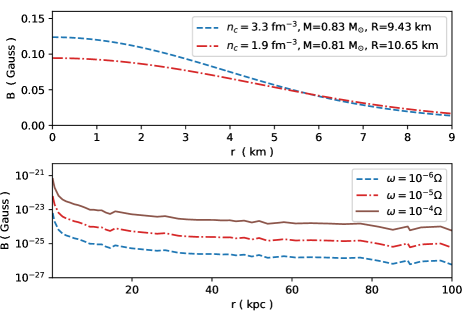
Figure 1: The upper panel shows the seed magnetic field inside an ideal neutron star whose stellar fluid is revolving 500 times a second. For a central neutron number density of $3.3$ fm^-3, the star has a seed magnetic field of around $0.12$ Gauss at its center. Here we have taken ${\bf\mu_{D}}=9.66\times 10^{-31}$ J/Gauss for neutrons. The lower panel shows estimated seed magnetic field from the observed rotation curve of the Milky Way galaxy at current epoch for different compactness.

VIII Rotating Galaxy

The seed magnetism studied here would arise in all rotating astrophysical bodies including the galaxies. For example, the angular velocity $\Omega$ of the Milky Way galaxy varies from $10^{-14}$ to $10^{-17}$ rev.s^-1 in the distance range $0.2-100$ kpc from the galactic center, as implied by its observed rotation curve Bhattacharjee et al. (2014). It also implies the dominant presence of dark matter in the galaxy where stellar mass contributes only around $4\%$ of its total mass of $\sim 10^{12}M_{\odot}$ McMillan (2016). The corresponding frame-dragging velocity $\omega$ can be obtained in principle by solving Einstein equation with a non-trivial galactic matter distribution. However, a lower bound on $\omega$ can be obtained by using the vacuum solution $\omega=2GJ/R^{3}$ at the edge of galaxy with a spherical dark matter hallo. Assuming Newtonian expression of angular momentum $J$, we can approximate $\omega\sim(2GM/R)~{}\Omega$. The observed mass $M$ of the Milky Way implies a compactness ratio $2GM/R\simeq 10^{-6}$ at $R=100$ kpc. Inside the galaxy the compactness ratio is expected to be higher. For different choices of compactness ratio, the galactic seed magnetic field is plotted in the FIG. 1. As earlier, a seed field is important in a proto-galaxy in the early universe. Using the covariant scaling of magnetic field as $B(1+z)^{2}$, the seed field in the proto-galaxy at a redshift $z\sim 9$, would be between $10^{-19}-10^{-24}$ Gauss. In comparison, the astrophysical battery mechanism of Biermann produces $\sim 10^{-21}$ Gauss seed field at a proto-galactic stage which has been shown to be sufficient to produce presently observed microgauss magnetic field Kulsrud et al. (1997). Inside a galaxy, additional smaller scale seed fields of varied magnitude would be created due to subsequent formation of different rotating stars.

IX Discussions

We have shown that the frame-dragging effect unavoidably leads to a seed magnetic field due to the spin-degeneracy breaking of fermions. The seed field is shown to be sufficient in strength and is coherent over a very large length scale to be astro-physically relevant. The conservation of angular momentum ensures that the seed field is sustained over a very long period of time. Further, the seed field arises only after rotating bodies are formed during the structure formation, without affecting the early universe physics. Therefore, the mechanism shown here are free from the shortcomings of other studied mechanisms in the literature. For simplicity here we have considered an ensemble of non-interacting neutrons. An ensemble of interacting neutrons would lead to relatively higher mass stars Hossain and Mandal (2021b) but without significantly affecting the result shown here. We note that particle and anti-particle asymmetry for neutrinos moving around a rotating black hole has been studied earlier Mukhopadhyay (2005).