Search for hidden-charm pentaquark states in three-body final states

Abstract

The three pentaquark states, $P_{c}(4312)$, $P_{c}(4440)$ and $P_{c}(4457)$, discovered by the LHCb Collaboration in 2019, are often interpreted as $\bar{D}^{(\ast)}\Sigma_{c}$ molecules. Together with their four $\bar{D}^{(*)}\Sigma_{c}^{\ast}$ partners dictated by heavy quark spin symmetry they represent a complete multiplet of hadronic molecules of $\bar{D}^{(\ast)}\Sigma_{c}^{(\ast)}$. The pentaquark states were observed in the $J/\psi p$ invariant mass distributions of the $\Lambda_{b}\rightarrow J/\psi pK$ decay. It is widely recognized that to understand their nature, other discovery channels play an important role. In this work, we investigate two three-body decay modes of the $\bar{D}^{(\ast)}\Sigma_{c}^{(\ast)}$ molecules. The tree-level modes proceed via off-shell $\Sigma_{c}^{(\ast)}$ baryons, $\bar{D}^{(\ast)}\Sigma_{c}^{(\ast)}\to\bar{D}^{(\ast)}\left(\Sigma_{c}^{(\ast)}\to\Lambda_{c}\pi\right)\to\bar{D}^{(\ast)}\Lambda_{c}\pi$, while the triangle-loop modes proceed through $\bar{D}^{\ast}\Sigma_{c}^{(\ast)}\to J/\psi N\pi$, $\eta_{c}N\pi$ via $\bar{D}\Sigma_{c}^{(\ast)}$ rescattering to $J/\psi N$ and $\eta_{c}N$. Our results indicate that the decay widths of the $P_{c}(4457)$ and $\bar{D}^{(\ast)}\Sigma_{c}^{\ast}$ states into $\bar{D}^{(\ast)}\Lambda_{c}\pi$ are several MeV, as a result can be observed in the upcoming Run 3 and Run 4 of LHC. The partial decay widths into $\bar{D}^{(\ast)}\Lambda_{c}\pi$ of the $P_{c}(4312)$ and $P_{c}(4440)$ states range from tens to hundreds of keV. In addition, the partial decay widths of $\bar{D}^{\ast}\Sigma_{c}$ molecules into $J/\psi N\pi$ and $\eta_{c}N\pi$ are several keV and tens of keV, respectively, and the partial decay widths of $\bar{D}^{\ast}\Sigma_{c}^{\ast}$ molecules into $J/\psi N\pi$ vary from several keV to tens of keV. In particular, we show that the spin-5/2 $\bar{D}^{\ast}\Sigma_{c}^{\ast}$ state can be searched for in the $J/\psi N\pi$ and $\bar{D}^{\ast}\Lambda_{c}\pi$ invariant mass distributions, while the latter one is more favorable. These three-body decay modes of the pentaquark states are of great value to further observations of the pentaquark states and to a better understanding of their nature.

I Introduction

The existence of hidden-charm pentaquark states was predicted about ten years ago Wu et al. (2010, 2011); Wang et al. (2011); Yang et al. (2012); Yuan et al. (2012); Wu et al. (2012); Garcia-Recio et al. (2013); Xiao et al. (2013); Uchino et al. (2016); Karliner and Rosner (2015). In 2015, the LHCb Collaboration observed two pentaquark states, named as $P_{c}(4380)$ and $P_{c}(4450)$, in the $J/\psi p$ invariant mass distributions of the $\Lambda_{b}\to J/\psi pK$ decay Aaij et al. (2015). In 2019, the LHCb Collaboration updated their analysis with ten times more data, showing that the original $P_{c}(4450)$ state splits into two states, $P_{c}(4440)$ and $P_{c}(4457)$, and in addition a new state $P_{c}(4312)$ is discovered Aaij et al. (2019a). The masses and decay widths of the three states are

$$M_{P_{c}(4312)} = 4311.9\pm 0.7^{+6.8}_{-0.6}~{}\mbox{MeV}\quad\quad\Gamma_{P_{c}(4312)}=9.8\pm 2.7^{+3.7}_{-4.5}~{}\mbox{MeV},$$

$$M_{P_{c}(4440)} = 4440.3\pm 1.3^{+4.1}_{-4.7}~{}\mbox{MeV}\quad\quad\Gamma_{P_{c}(4440)}=20.6\pm 4.9^{+8.7}_{-10.1}~{}\mbox{MeV},$$ (1)

$$M_{P_{c}(4457)} = 4457.3\pm 0.6^{+4.1}_{-1.7}~{}\mbox{MeV}\quad\quad\Gamma_{P_{c}(4457)}=6.4\pm 2.0^{+5.7}_{-1.9}~{}\mbox{MeV}.$$

Two more pentaquark states were reported in the following years, though only with a significance of about 3$\sigma$. A hidden-charm pentaquark with strangeness, $P_{cs}(4459)$, is visible in the $J/\psi\Lambda$ invariant mass spectrum Aaij et al. (2021), and a hidden-charm pentaquark $P_{c}(4337)$ was found in both the $J/\psi p$ and $J/\psi\bar{p}$ invariant mass spectrum Aaij et al. (2022a). The former has been predicted by many studies as the $SU(3)$-flavor partner of the pentaquark states, $P_{c}(4312)$, $P_{c}(4380)$, $P_{c}(4440)$, and $P_{c}(4457)$ Chen et al. (2016, 2017); Shen et al. (2019); Xiao et al. (2019a); Wang et al. (2020a), while the latter is more difficult to understand. It could be a $\chi_{c0}(1S)p$ bound state Yan et al. (2022), a compact multiquark state Deng (2022), a cusp effect Nakamura et al. (2021), or a reflection effect Wang et al. (2021). Therefore, we will leave a study of $P_{cs}(4459)$ and $P_{c}(4337)$ to a future work.

Trying to understand the nature of the pentaquark states has led to intensive theoretical studies. In Refs. Liu et al. (2019, 2021) we have employed both an effective field theory (EFT) and the one-boson-exchange (OBE) model to describe the three pentaquark states as $\bar{D}^{(\ast)}\Sigma_{c}$ molecules by reproducing their masses, which is later confirmed by many other theoretical studies Chen et al. (2019a); He (2019); Chen et al. (2019b); Xiao et al. (2019b); Yamaguchi et al. (2020); Pavon Valderrama (2019); Du et al. (2020); He and Chen (2019); Wang et al. (2020b). In addition to the $\bar{D}^{(\ast)}\Sigma_{c}$ channel, the role of the $\bar{D}\Lambda_{c1}$ channel has been studied in relation with the $P_{c}(4457)$ state Burns and Swanson (2019); Peng et al. (2021a); Yalikun et al. (2021). In Refs. Xiao et al. (2019c); Lin and Zou (2019) with the effective Lagrangian approach the authors reproduced the decay widths of the pentaquark states in the hadronic molecular picture. With the same approach, Wu et al. calculated the ratios of the production rates of the pentaquark states in the $\Lambda_{b}$ decays, and obtained results in agreement with the LHCb measurements Wu and Chen (2019). Although the molecular interpretation is the most popular, other explanations are also available, e.g., hadro-charmonia Eides et al. (2020), compact pentaquark states Ali and Parkhomenko (2019); Mutuk (2019); Wang (2020); Cheng and Liu (2019); Weng et al. (2019); Zhu et al. (2019); Pimikov et al. (2020); Ruangyoo et al. (2022); Deng (2022), virtual states Fernández-Ramírez et al. (2019) or double triangle singularities Nakamura (2021).

To investigate the molecular nature of the pentaquark states, many other methods have been proposed. Historically, the existence of the $\Omega$ baryon indeed verified the quark model, where the $SU(3)$-flavor symmetry plays an important role. Following the same principle, among others, we proposed that, if future experiments could discover the four heavy quark spin symmetry (HQSS) partners of the $\bar{D}^{(\ast)}\Sigma_{c}^{\ast}$ molecules, it would support their molecular nature Liu et al. (2019). Apart from HQSS, their $SU(3)$-flavor symmetry partners Xiao et al. (2019a); Wang et al. (2020a) and heavy quark flavor symmetry partners Wang et al. (2019); Azizi et al. (2021) have been predicted, the existence of which can also support the molecular nature of the pentaquark states. In our previous work Pan et al. (2020), we showed that one can study instead the $\Xi_{cc}^{(\ast)}\Sigma_{c}^{(\ast)}$ system, because it can be related to the $\bar{D}^{(\ast)}\Sigma_{c}^{(\ast)}$ system via heavy antiquark diquark symmetry (HADS). In addition, lattice QCD simulations can provide valuable information to understand the pentaquark states, but a complete simulation of the pentaquark system with all the relevant coupled channels is complicated Skerbis and Prelovsek (2019); Sugiura et al. (2019). Recently, we predicted the existence of a three-body hadronic molecule $\Sigma_{c}\bar{D}\bar{K}$ Wu et al. (2021), which can be viewed as an excited state of the $P_{cs}(4459)$ state. If the $\Sigma_{c}\bar{D}\bar{K}$ molecule is discovered in the future, it will provide a non-trivial check on the molecular nature of the pentaquark states.

The decay and production mechanisms of the pentaquark states have also attracted considerable attention, which can offer valuable means to reveal their nature. In Ref. Sakai et al. (2019), assuming the pentaquark states as hadronic molecules, Sakai et al. found that the decay width of $P_{c}(4312)\to\eta_{c}p$ is about three times larger than that of $P_{c}(4312)\to J/\psi p$, in agreement with the results of the quark interchange model Wang et al. (2020b). However, if $P_{c}(4312)$ is regarded as a compact pentaquark state, it will dominantly decay into $\bar{D}^{\ast}\Lambda_{c}$ rather than $\eta_{c}p$ Weng et al. (2019). In Ref.Guo et al. (2019), Guo et al. estimated that the branching ratio Br$(P_{c}(4457)\to J/\psi\Delta)$/Br$(P_{c}(4457)\to J/\psi p)$ ranges from a few percent to about $30\%$ in the molecular picture, which shows a larger isospin breaking in comparison with the decays of ordinary hadrons. As a result, experimental measurements of such branching ratios are of great value to reveal the internal structure of the pentaquark states. In Ref. Chen et al. (2022), Chen et al. estimated the production rates of $P_{c}(4312)$, $P_{c}(4440)$ and $P_{c}(4457)$ in $pp$ collisions using the constrained phasespace coalescence model and the parton and hadron cascade (PACIAE) model. Their results show that the production rates of the pentaquark states, the nucleuslike states, and the hadronic molecular states are of the same order. In Ref. Yang and Guo (2021), Yang et al. estimated the production rates of $P_{c}$’s in lepton-proton processes, where the $P_{c}$’s are treated as hadronic molecules.

To further explore the decay mechanism of the pentaquark states in the molecular picture, in this work we study the three-body decays of the seven $\bar{D}^{(\ast)}\Sigma_{c}^{(\ast)}$ pentaquark states. The decay mechanism of the $\bar{D}^{(\ast)}\Sigma_{c}^{(\ast)}$ molecules is similar to that of the $T_{cc}$ state recently discovered by the LHCb Collaboration Aaij et al. (2022b, c), where the decay of $T_{cc}$ in the molecular picture proceeds via the off-shell $D^{\ast}$ meson Meng et al. (2021); Ling et al. (2022); Chen et al. (2021); Feijoo et al. (2021); Yan and Valderrama (2022); Fleming et al. (2021); Albaladejo (2022); Du et al. (2022); Mikhasenko (2022). As for the $\bar{D}^{(\ast)}\Sigma_{c}^{(\ast)}$ molecules, we will consider two three-body decay modes. The tree-level modes proceed via off-shell $\Sigma_{c}^{(\ast)}$ baryons, i.e. $\bar{D}^{(\ast)}\Sigma_{c}^{(\ast)}\to\bar{D}^{(\ast)}\left(\Sigma_{c}^{(\ast)}\to\Lambda_{c}\pi\right)\to\bar{D}^{(\ast)}\Lambda_{c}\pi$, while the triangle-loop modes proceed through $\bar{D}^{\ast}\Sigma_{c}^{(\ast)}\to J/\psi N\pi$, $\eta_{c}N\pi$ via $\bar{D}\Sigma_{c}^{(\ast)}$ rescattering to $J/\psi N$ or $\eta_{c}N$. We use the effective Lagrangian approach to estimate the decay widths of these two modes in this work. We hope that these decay modes can offer further insights into the nature of the pentaquark states.

This paper is organized as follows. In Sec. II, we introduce the coupled-channel contact-range EFT of $\eta_{c}N-J/\psi N-\bar{D}^{(\ast)}\Sigma_{c}^{(\ast)}$ for the pentaquark system as well as present the decay amplitudes of the $\bar{D}^{(\ast)}\Sigma_{c}^{(\ast)}$ molecules via tree-level and triangle-loop diagrams using the effective Lagrangian approach. In Sec. III, we present the mass spectrum of $\bar{D}^{(\ast)}\Sigma_{c}^{(\ast)}$, their relevant couplings and the decay widths of the $\bar{D}^{(\ast)}\Sigma_{c}^{(\ast)}$ molecules into $\bar{D}^{(\ast)}\Lambda_{c}\pi$ and $J/\psi(\eta_{c})N\pi$. Finally, this paper ends with a short summary in Sec. IV.

II Theoretical framework

The three-body decay modes of the $\bar{D}^{(\ast)}\Sigma_{c}^{(\ast)}$ molecules can proceed via two types of Feynman diagrams as shown in Fig. 1 and Fig. 2: tree-level diagrams and triangle-loop diagrams. The binding energies of the $\bar{D}^{\ast}\Sigma_{c}^{(\ast)}$ molecules relative to their mass thresholds are around 4-20 MeV Liu et al. (2019); Zyla et al. (2020a), while the mass thresholds of $\bar{D}\pi\Sigma_{c}^{(\ast)}$ are 5 MeV less than those of $\bar{D}^{\ast}\Sigma_{c}^{(\ast)}$, which implies that the $\bar{D}^{\ast}\Sigma_{c}^{(\ast)}$ molecules decaying into $\bar{D}\pi\Sigma_{c}^{(\ast)}$ via off-shell $\bar{D}^{\ast}$ meson are heavily suppressed or forbidden. The phase space of $\Sigma_{c}^{(\ast)}\to\Lambda_{c}\pi$ is more than 30 MeV, so that the tree-level decays of $\bar{D}^{(\ast)}\Sigma_{c}^{(\ast)}\to\bar{D}^{(\ast)}\left(\Sigma_{c}^{(\ast)}\to\Lambda_{c}\pi\right)\to\bar{D}^{(\ast)}\Lambda_{c}\pi$ are allowed, as shown in Fig. 1. The rescattering between final states $\bar{D}^{(\ast)}\Lambda_{c}\pi$ can form the decay modes of the triangle-loop diagrams, which are small due to the fact that the loop diagrams are suppressed with respect to the tree-level diagrams Yan and Valderrama (2022), satisfying the power counting of EFT. Although the decay mode of $\bar{D}^{\ast}\to\bar{D}\pi$ is not allowed at tree level, their final states $\bar{D}\Sigma_{c}^{(\ast)}$ would couple to the $J/\psi N$ and $\eta_{c}N$ channels according to HQSS Sakai et al. (2019). Therefore, considering the final-state interactions, it would lead to the decay modes via the triangle-loop mechanism as shown in Fig. 2.

\begin{overpic}[scale={0.09}]{tree.png} \put(12.0,26.0){$P_{c1}^{+}$} \par\put(40.0,3.0){$D^{-}$} \par\put(38.0,33.0){$\Sigma_{c}^{++}$} \put(68.0,52.0){$\Lambda_{c}^{+}$} \put(69.0,20.0){$\pi^{+}$} \put(45.0,-6.0){(a1)} \end{overpic} \begin{overpic}[scale={0.09}]{tree.png} \put(12.0,26.0){$P_{c1}^{+}$} \par\put(38.0,3.0){$\bar{D}^{0}$} \par\put(39.0,33.0){$\Sigma_{c}^{+}$} \put(68.0,52.0){$\Lambda_{c}^{+}$} \put(69.0,20.0){$\pi^{0}$} \put(45.0,-6.0){(a2)} \end{overpic} \begin{overpic}[scale={0.09}]{tree.png} \put(12.0,26.0){$P_{c2}^{+}$} \par\put(40.0,3.0){$D^{-}$} \par\put(35.0,33.0){$\Sigma_{c}^{\ast++}$} \put(68.0,52.0){$\Lambda_{c}^{+}$} \put(69.0,20.0){$\pi^{+}$} \put(45.0,-6.0){(b1)} \end{overpic} \begin{overpic}[scale={0.09}]{tree.png} \put(12.0,26.0){$P_{c2}^{+}$} \par\put(38.0,3.0){$\bar{D}^{0}$} \par\put(38.0,33.0){$\Sigma_{c}^{\ast+}$} \put(68.0,52.0){$\Lambda_{c}^{+}$} \put(69.0,20.0){$\pi^{0}$} \put(45.0,-6.0){(b2)} \end{overpic}

\begin{overpic}[scale={0.09}]{tree.png} \put(8.0,27.0){$P_{c3|c4}^{+}$} \par\put(36.0,3.0){$D^{\ast-}$} \par\put(38.0,33.0){$\Sigma_{c}^{++}$} \put(68.0,52.0){$\Lambda_{c}^{+}$} \put(69.0,20.0){$\pi^{+}$} \put(45.0,-6.0){(c1)} \end{overpic} \begin{overpic}[scale={0.09}]{tree.png} \put(8.0,27.0){$P_{c3|c4}^{+}$} \par\put(35.0,3.0){$\bar{D}^{\ast 0}$} \par\put(39.0,33.0){$\Sigma_{c}^{+}$} \put(68.0,52.0){$\Lambda_{c}^{+}$} \put(69.0,20.0){$\pi^{0}$} \put(45.0,-6.0){(c2)} \end{overpic} \begin{overpic}[scale={0.09}]{tree.png} \put(3.0,27.0){$P_{c5|c6|c7}^{+}$} \par\put(36.0,3.0){$D^{\ast-}$} \par\put(35.0,33.0){$\Sigma_{c}^{\ast++}$} \put(68.0,52.0){$\Lambda_{c}^{+}$} \put(69.0,20.0){$\pi^{+}$} \put(45.0,-6.0){(d1)} \end{overpic} \begin{overpic}[scale={0.09}]{tree.png} \put(3.0,27.0){$P_{c5|c6|c7}^{+}$} \par\put(35.0,3.0){$\bar{D}^{\ast 0}$} \par\put(38.0,33.0){$\Sigma_{c}^{\ast+}$} \put(68.0,52.0){$\Lambda_{c}^{+}$} \put(69.0,20.0){$\pi^{0}$} \put(45.0,-6.0){(d2)} \end{overpic}

Figure 1: Tree-level diagrams for the decays of $P_{c1}\to\bar{D}\Sigma_{c}\to\bar{D}\Lambda_{c}\pi$ (a), $P_{c2}\to\bar{D}\Sigma_{c}^{\ast}\to\bar{D}\Lambda_{c}\pi$ (b), $P_{c3|c4}\to\bar{D}^{\ast}\Sigma_{c}\to\bar{D}^{\ast}\Lambda_{c}\pi$ (c) and $P_{c5|c6|c7}\to\bar{D}^{\ast}\Sigma_{c}^{\ast}\to\bar{D}^{\ast}\Lambda_{c}\pi$ (d).

\begin{overpic}[scale={0.26}]{tr1.png} \put(11.0,34.0){$P_{c3|c4}^{+}$} \par\put(34.0,14.0){$\Sigma_{c}^{+}$} \par\put(33.0,39.0){$\bar{D}^{\ast 0}$} \put(53.0,28.0){$D^{-}$} \put(67.0,48.0){$\pi^{+}$} \put(60.0,14.0){$J/\psi(\eta_{c})$} \put(55.0,5.0){$n$} \put(45.0,0.0){(a1)} \end{overpic}	\begin{overpic}[scale={0.26}]{tr1.png} \put(11.0,34.0){$P_{c3|c4}^{+}$} \par\put(34.0,14.0){$\Sigma_{c}^{+}$} \par\put(33.0,39.0){$\bar{D}^{\ast 0}$} \put(53.0,28.0){$\bar{D}^{0}$} \put(67.0,48.0){$\pi^{0}$} \put(60.0,14.0){$J/\psi(\eta_{c})$} \put(55.0,5.0){$p$} \put(45.0,0.0){(a2)} \end{overpic}	\begin{overpic}[scale={0.26}]{tr1.png} \put(11.0,34.0){$P_{c3|c4}^{+}$} \par\put(32.0,14.0){$\Sigma_{c}^{++}$} \par\put(33.0,39.0){$D^{\ast-}$} \put(53.0,28.0){$D^{-}$} \put(67.0,48.0){$\pi^{0}$} \put(60.0,14.0){$J/\psi(\eta_{c})$} \put(55.0,5.0){$p$} \put(45.0,0.0){(a3)} \end{overpic}
\begin{overpic}[scale={0.26}]{tr1.png} \put(8.0,34.0){$P_{c5|c6|c7}^{+}$} \par\put(33.0,14.0){$\Sigma_{c}^{\ast+}$} \par\put(33.0,39.0){$\bar{D}^{\ast 0}$} \put(53.0,28.0){$D^{-}$} \put(67.0,48.0){$\pi^{+}$} \put(59.0,13.0){$J/\psi$} \put(55.0,5.0){$n$} \put(45.0,0.0){(b1)} \end{overpic}	\begin{overpic}[scale={0.26}]{tr1.png} \put(8.0,34.0){$P_{c5|c6|c7}^{+}$} \par\put(33.0,14.0){$\Sigma_{c}^{\ast+}$} \par\put(33.0,39.0){$\bar{D}^{\ast 0}$} \put(53.0,28.0){$\bar{D}^{0}$} \put(67.0,48.0){$\pi^{0}$} \put(59.0,13.0){$J/\psi$} \put(55.0,5.0){$p$} \put(45.0,0.0){(b2)} \end{overpic}	\begin{overpic}[scale={0.26}]{tr1.png} \put(8.0,34.0){$P_{c5|c6|c7}^{+}$} \par\put(30.0,14.0){$\Sigma_{c}^{\ast++}$} \par\put(33.0,39.0){$D^{\ast-}$} \put(53.0,28.0){$D^{-}$} \put(67.0,48.0){$\pi^{0}$} \put(59.0,13.0){$J/\psi$} \put(55.0,5.0){$p$} \put(45.0,0.0){(b3)} \end{overpic}

Figure 2: Triangle-loop diagrams for the decays of $P_{c3|c4}\to\bar{D}^{\ast}\Sigma_{c}\to J/\psi(\eta_{c})N\pi$ (a) and $P_{c5|c6|c7}\to\bar{D}^{\ast}\Sigma_{c}^{\ast}\to J/\psi N\pi$ (b) via the rescattering of final states.

To calculate the Feynman diagrams of Figs. 1 and 2, we have to describe the interactions related to each vertex, which can be classified into three categories. The first category involves the interactions between the hadronic molecules and their constituents. In this work, the seven $\bar{D}^{(\ast)}\Sigma_{c}^{(\ast)}$ hadronic molecules are denoted by $P_{c1}$, $P_{c2}$, $\ldots$, $P_{c7}$, following the order of scenario A of Table I in Ref. Liu et al. (2019) (see also Table II). Here, we should note that $P_{c1}$, $P_{c3}$, and $P_{c5}$ have $J=1/2$, $P_{c2}$ and $P_{c4}$ have $J=3/2$, and $P_{c7}$ has $J=5/2$, respectively. Their interactions with the corresponding constituents are described by the following Lagrangians Lin and Zou (2019):

$$\mathcal{L}_{P_{c1}\bar{D}\Sigma_{c}} = -ig_{P_{c1}\bar{D}\Sigma_{c}}\bar{\Sigma}_{c}\bar{D}P_{c1},$$

$$\mathcal{L}_{P_{c2}\bar{D}\Sigma_{c}^{\ast}} = -ig_{P_{c2}\bar{D}\Sigma_{c}^{\ast}}\bar{\Sigma}_{c\mu}^{\ast}\bar{D}P_{c2}^{\mu},$$

$$\mathcal{L}_{P_{c3}\bar{D}^{\ast}\Sigma_{c}} = g_{P_{c3}\bar{D}^{\ast}\Sigma_{c}}\bar{\Sigma}_{c}\gamma^{5}\widetilde{\gamma}^{\mu}\bar{D}^{\ast}_{\mu}P_{c3},$$

$$\mathcal{L}_{P_{c4}\bar{D}^{\ast}\Sigma_{c}} = g_{P_{c4}\bar{D}^{\ast}\Sigma_{c}}\bar{\Sigma}_{c}\bar{D}^{\ast}_{\mu}P_{c4}^{\mu},$$ (2)

$$\mathcal{L}_{P_{c5}\bar{D}^{\ast}\Sigma_{c}^{\ast}} = g_{P_{c5}\bar{D}^{\ast}\Sigma_{c}^{\ast}}\bar{\Sigma}_{c}^{\ast\mu}\bar{D}^{\ast}_{\mu}P_{c5},$$

$$\mathcal{L}_{P_{c6}\bar{D}^{\ast}\Sigma_{c}^{\ast}} = g_{P_{c6}\bar{D}^{\ast}\Sigma_{c}^{\ast}}\bar{\Sigma}_{c\mu}^{\ast}\bar{D}^{\ast}_{\nu}\gamma^{5}\widetilde{\gamma}^{\nu}P_{c6}^{\mu},$$

$$\mathcal{L}_{P_{c7}\bar{D}^{\ast}\Sigma_{c}^{\ast}} = g_{P_{c7}\bar{D}^{\ast}\Sigma_{c}^{\ast}}\bar{\Sigma}_{c\mu}^{\ast}\bar{D}^{\ast}_{\nu}P_{c7}^{\mu\nu},$$

where $g_{P_{c1...c7}\bar{D}^{(\ast)}\Sigma_{c}^{(\ast)}}$ are the couplings, which will be determined by the EFT approach described below. $\widetilde{\gamma}^{\mu}$ is defined as $\widetilde{\gamma}^{\mu}=(g^{\mu\nu}-p^{\mu}p^{\nu}/p^{2}){\gamma_{\nu}}$, where $p$ is the momentum of the initial $P_{c}$ states.

The second category involves the decays of the molecular constituents, i.e., $\Sigma_{c}^{(\ast)}\to\Lambda_{c}\pi$ and $\bar{D}^{\ast}\to\bar{D}\pi$. The Lagrangians describing $\Sigma_{c}^{(\ast)}\to\Lambda_{c}\pi$ read

$$\mathcal{L}_{\pi\Lambda_{c}{\Sigma}_{c}} = -i\frac{g_{\pi\Lambda_{c}{\Sigma}_{c}}}{f_{\pi}}~{}\bar{\Lambda}_{c}\gamma^{\mu}\gamma_{5}\partial_{\mu}\vec{\phi}_{\pi}\cdot\vec{\tau}{\Sigma}_{c},$$ (3)

$$\mathcal{L}_{\pi\Lambda_{c}{\Sigma}_{c}^{*}} = \frac{g_{\pi\Lambda_{c}{\Sigma}_{c}^{*}}}{f_{\pi}}~{}\bar{\Lambda}_{c}\partial^{\mu}\vec{\phi}_{\pi}\cdot\vec{\tau}{\Sigma}_{c\mu}^{*},$$

where the pion decay constant $f_{\pi}=132$ MeV. The couplings $g_{\pi\Lambda_{c}{\Sigma}_{c}}$ and $g_{\pi\Lambda_{c}{\Sigma}_{c}^{*}}$ can be determined by reproducing the corresponding experimental data. With the decay widths of $\Sigma_{c}^{++,+,0}\to\Lambda_{c}^{+}\pi^{+,0,-}$ and $\Sigma_{c}^{\ast++,+,0}\to\Lambda_{c}^{+}\pi^{+,0,-}$ being 1.89, 2.3, 1.83 MeV and 14.78, 17.2, 15.3 MeV, respectively Zyla et al. (2020b), we obtain the corresponding couplings $g_{\pi\Lambda_{c}{\Sigma}_{c}}=0.538,0.554,0.532$ and $g_{\pi\Lambda_{c}{\Sigma}_{c}^{*}}=0.984,1.043,1.001$, consistent with other works Liu and Oka (2012); Cheng and Chua (2015). In addition, we find that the two kinds of couplings approximately satisfy the relationship $g_{\pi\Lambda_{c}{\Sigma}_{c}^{*}}=\sqrt{3}g_{\pi\Lambda_{c}{\Sigma}_{c}}$, which can be derived from the quark model Liu and Oka (2012). The Lagrangian describing the $D^{\ast}$ decay into $D\pi$ is

$$\mathcal{L}_{DD^{\ast}\pi} = -ig_{DD^{\ast}\pi}(D\partial^{\mu}\pi D^{\ast{\dagger}}_{\mu}-D_{\mu}^{*}\partial^{\mu}\pi D^{{\dagger}}),$$ (4)

where the coupling is determined to be $g_{D^{\ast+}D^{0}\pi^{+}}=16.818$ by reproducing the decay width of $D^{\ast+}\to D^{0}\pi^{+}$ Zyla et al. (2020b). Experimentally, there exists only an upper limit $\Gamma<2.1$ MeV for the $D^{\ast 0}$ width. Thus we turn to the quark model Rosner (2013), where the strong decay width of $D^{\ast 0}$ is estimated to be $\Gamma_{D^{\ast 0}\to D^{0}\pi^{0}}=34.658$ keV.  With these numbers, we obtain the coupling $g_{D^{\ast 0}D^{0}\pi^{0}}=11.688$. It is clear that the strong couplings approximately satisfy isospin symmetry.

The last category involves the rescattering of final states, which is described by the scattering amplitude $T$ and is responsible for the dynamical generation of the pentaquark states. It can be obtained by solving the Lippmann-Schwinger equation

$$T=(1-VG)^{-1}V,$$ (5)

where $V$ is the coupled-channel potential determined by the contact EFT approach described below, and $G$ is the two-body propagator. Here to avoid the ultraviolet divergence induced by evaluating the loop function $G$ and keep the unitarity of the $T$ matrix , we include a regulator of Gaussian form $F(q^{2},k)=e^{-2q^{2}/\Lambda^{2}}/e^{-2k^{2}/\Lambda^{2}}$ in the integral as

$$G(\sqrt{s})=2m_{1}\int\frac{d^{3}q}{(2\pi)^{3}}\frac{\omega_{1}+\omega_{2}}{2~{}\omega_{1}\omega_{2}}\frac{F(q^{2},k)}{(\sqrt{s})^{2}-(\omega_{1}+\omega_{2})^{2}+i\varepsilon},$$ (6)

where $\sqrt{s}$ is the total energy in the center-of-mass (c.m.) frame of $m_{1}$ and $m_{2}$, $\omega_{i}=\sqrt{m_{i}^{2}+q^{2}}$ is the energy of the particle, $\Lambda$ is the momentum cutoff, and the c.m. momentum $k$ is ,

$$k=\frac{\sqrt{{s}-(m_{1}+m_{2})^{2}}\sqrt{s-(m_{1}-m_{2})^{2}}}{2{\sqrt{s}}}.$$ (7)

The dynamically generated pentaquark states correspond to poles in the unphysical sheet, which are below the $\bar{D}^{(\ast)}\Sigma_{c}^{(\ast)}$ mass thresholds and above the mass thresholds of $J/\psi N$ and $\eta_{c}N$. The effect of scattering amplitude $T$ passing $\sqrt{s}$ to unphysical sheet has consequences only for the loop functions. We denote the loop function in physical sheet and unphysical sheet as $G_{I}(\sqrt{s})$ and $G_{II}(\sqrt{s})$, respectively, which are related by $G_{II}(\sqrt{s})=G_{I}(\sqrt{s})-2i\mathrm{Im}~{}G_{I}(\sqrt{s})$ Oller and Oset (1997); Roca et al. (2005). The imaginary part of Eq. (6) can be derived via Plemelj-Sokhotski formula, i.g., $\mathrm{Im}~{}G(\sqrt{s})=-\frac{2m_{1}}{8\pi}\frac{k}{\sqrt{s}}$, and then the Eq. (6) in the unphysical sheet is written as

$$G_{II}(\sqrt{s})=G_{I}(\sqrt{s}){+~{}i\frac{2m_{1}}{4\pi}\frac{k}{\sqrt{s}}}.$$ (8)

To study the decays of the $\bar{D}^{(*)}\Sigma_{c}^{(*)}$ molecules, we first extend our single-channel contact-range EFT Liu et al. (2019) to include the $J/\psi N$ and $\eta_{c}N$ channels. This can be easily achieved by utilizing HQSS in the following way. First, we express the spin wave function of the $\bar{D}^{(\ast)}\Sigma_{c}^{(\ast)}$ pairs in terms of the spins of the heavy quarks $s_{1H}$ and $s_{2H}$ and those of the light quark(s) (often referred to as brown muck Isgur and Wise (1992); Flynn and Isgur (1992)) $s_{1L}$ and $s_{2L}$, where 1 and 2 denote $\bar{D}^{(*)}$ and $\Sigma_{c}^{(*)}$, respectively, via the following spin coupling formula,

$$|s_{1l},s_{1h},j_{1};s_{2l},s_{2h},j_{2};J\rangle=$$ (9)

$$\sqrt{(2j_{1}+1)(2j_{2}+1)(2s_{L}+1)(2s_{H}+1)}\left(\begin{matrix}s_{1l}&s_{2l}&s_{L}\\ s_{1h}&s_{2h}&s_{H}\\ j_{1}&j_{2}&J\end{matrix}\right)|s_{1l},s_{2l},s_{L};s_{1h},s_{2h},s_{H};J\rangle.$$

More explicitly, for the seven $\bar{D}^{(\ast)}\Sigma_{c}^{(\ast)}$ states, the decompositions read

$$|\Sigma_{c}\bar{D}(1/2^{-})\rangle = \frac{1}{2}0_{H}\otimes{1/2}_{L}+\frac{1}{2\sqrt{3}}1_{H}\otimes{1/2}_{L}+\sqrt{\frac{2}{3}}1_{H}\otimes{3/2}_{L},$$ (10)

$$|\Sigma_{c}^{\ast}\bar{D}(3/2^{-})\rangle = -\frac{1}{2}0_{H}\otimes{3/2}_{L}+\frac{1}{\sqrt{3}}1_{H}\otimes{1/2}_{L}+\frac{\sqrt{\frac{5}{3}}}{2}1_{H}\otimes{3/2}_{L},$$

$$|\Sigma_{c}\bar{D}^{\ast}(1/2^{-})\rangle = \frac{1}{2\sqrt{3}}0_{H}\otimes{1/2}_{L}+\frac{5}{6}1_{H}\otimes{1/2}_{L}-\frac{\sqrt{2}}{3}1_{H}\otimes{3/2}_{L},$$

$$|\Sigma_{c}\bar{D}^{\ast}(3/2^{-})\rangle = \frac{1}{\sqrt{3}}0_{H}\otimes{3/2}_{L}-\frac{1}{3}1_{H}\otimes{1/2}_{L}+\frac{\sqrt{5}}{3}1_{H}\otimes{3/2}_{L},$$

$$|\Sigma_{c}^{\ast}\bar{D}^{\ast}(1/2^{-})\rangle = \sqrt{\frac{2}{3}}0_{H}\otimes{1/2}_{L}-\frac{\sqrt{2}}{3}1_{H}\otimes{1/2}_{L}-\frac{1}{3}1_{H}\otimes{3/2}_{L},$$

$$|\Sigma_{c}^{\ast}\bar{D}^{\ast}(3/2^{-})\rangle = \frac{\sqrt{\frac{5}{3}}}{2}0_{H}\otimes{3/2}_{L}+\frac{\sqrt{5}}{3}1_{H}\otimes{1/2}_{L}-\frac{1}{6}1_{H}\otimes{3/2}_{L},$$

$$|\Sigma_{c}^{\ast}\bar{D}^{\ast}(5/2^{-})\rangle = 1_{H}\otimes{3/2}_{L}.$$

In the heavy quark limit, the $\bar{D}^{(\ast)}\Sigma_{c}^{(\ast)}$ interactions are independent of the spin of the heavy quark, and therefor the potentials can be parameterized by two coupling constants describing interactions between light quarks of spin 1/2 and 3/2, respectively, i.e., $F_{1/2}=\langle 1/2_{L}|V|1/2_{L}\rangle$ and $F_{3/2}=\langle 3/2_{L}|V|3/2_{L}\rangle$:

$$V_{\Sigma_{c}\bar{D}}(1/2^{-}) = \frac{1}{3}F_{1/2L}+\frac{2}{3}F_{3/2L},$$ (11)

$$V_{\Sigma_{c}^{\ast}\bar{D}}(3/2^{-}) = \frac{1}{3}F_{1/2L}+\frac{2}{3}F_{3/2L},$$

$$V_{\Sigma_{c}\bar{D}^{\ast}}(1/2^{-}) = \frac{7}{9}F_{1/2L}+\frac{2}{9}F_{3/2L},$$

$$V_{\Sigma_{c}\bar{D}^{\ast}}(3/2^{-}) = \frac{1}{9}F_{1/2L}+\frac{8}{9}F_{3/2L},$$

$$V_{\Sigma_{c}^{\ast}\bar{D}^{\ast}}(1/2^{-}) = \frac{8}{9}F_{1/2L}+\frac{1}{9}F_{3/2L},$$

$$V_{\Sigma_{c}^{\ast}\bar{D}^{\ast}}(3/2^{-}) = \frac{5}{9}F_{1/2L}+\frac{4}{9}F_{3/2L},$$

$$V_{\Sigma_{c}^{\ast}\bar{D}^{\ast}}(5/2^{-}) = F_{3/2L},$$

which can be rewritten as a combination of $C_{a}$ and $C_{b}$, i.e. $F_{1/2}=C_{a}-2C_{b}$ and $F_{3/2}=C_{a}+C_{b}$ Liu et al. (2019). For the inelastic potentials, one can see that there are three possible channels, $\eta_{c}N$, $J/\psi N$ and $J/\psi\Delta$. However, the $J/\psi\Delta$ channel is suppressed due to isospin symmetry breaking. From HQSS, the potentials between $\bar{D}^{(\ast)}\Sigma_{c}^{(\ast)}$ and $J/\psi N,\eta_{c}N$ are only related to the spin of the light quark $1/2$, denoted by one coupling: $g=\langle\bar{D}^{(\ast)}\Sigma_{c}^{(\ast)}|1_{H}\otimes 1/2_{L}\rangle=\langle\bar{D}^{(\ast)}\Sigma_{c}^{(\ast)}|0_{H}\otimes 1/2_{L}\rangle$. The potentials of $J/\psi N\to J/\psi N$, $J/\psi N\to\eta_{c}N$ and $\eta_{c}N\to\eta_{c}N$ are suppressed due to the Okubo-Zweig-Iizuka (OZI) rule, which is also supported by lattice QCD simulations Skerbis and Prelovsek (2019). In this work, we take the potentials of $V_{J/\psi(\eta_{c})N\to J/\psi(\eta_{c})N}=0$. In the following, we explicitly show the potentials for all the seven states.

For the $\eta_{c}N-J/\psi N-\bar{D}\Sigma_{c}$ and $\eta_{c}N-J/\psi N-\bar{D}\Sigma_{c}^{\ast}$ coupled channels, the contact-range potentials $V$ in matrix form read

$$V_{\eta_{c}N-J/\psi N-\bar{D}\Sigma_{c}}^{J=1/2}=\begin{pmatrix}0&0&\frac{1}{2}g\\ 0&0&\frac{1}{2\sqrt{3}}g\\ \frac{1}{2}g&\frac{1}{2\sqrt{3}}g&C_{a}\end{pmatrix},\quad V_{\eta_{c}N-J/\psi N-\bar{D}\Sigma_{c}^{\ast}}^{J=3/2}=\begin{pmatrix}0&0&0\\ 0&0&\frac{1}{\sqrt{3}}g\\ 0&\frac{1}{\sqrt{3}}g&C_{a}\end{pmatrix}.$$ (12)

For the $\eta_{c}N-J/\psi N-\bar{D}^{*}\Sigma_{c}$ coupled channels, the contact-range potentials for $J=1/2$ and $J=3/2$ read

$$V_{\eta_{c}N-J/\psi N-\bar{D}^{*}\Sigma_{c}}^{J=1/2}=\begin{pmatrix}0&0&\frac{1}{2\sqrt{3}}g\\ 0&0&\frac{5}{6}g\\ \frac{1}{2\sqrt{3}}g&\frac{5}{6}g&C_{a}-\frac{4}{3}C_{b}\end{pmatrix},\quad V_{\eta_{c}N-J/\psi N-\bar{D}^{*}\Sigma_{c}}^{J=3/2}=\begin{pmatrix}0&0&0\\ 0&0&-\frac{1}{3}g\\ 0&-\frac{1}{3}g&C_{a}+\frac{2}{3}C_{b}\end{pmatrix}.$$ (13)

Similarly for the $\eta_{c}N-J/\psi N-\bar{D}^{*}\Sigma_{c}^{*}$ coupled channels, they read

$$V_{\eta_{c}N-J/\psi N-\bar{D}^{*}\Sigma_{c}^{*}}^{J=1/2}=\begin{pmatrix}0&0&\sqrt{\frac{2}{3}}g\\ 0&0&-\frac{\sqrt{2}}{3}g\\ \sqrt{\frac{2}{3}}g&-\frac{\sqrt{2}}{3}g&C_{a}-\frac{5}{3}C_{b}\end{pmatrix},\quad V_{\eta_{c}N-J/\psi N-\bar{D}^{*}\Sigma_{c}^{*}}^{J=3/2}=\begin{pmatrix}0&0&0\\ 0&0&\frac{\sqrt{5}}{3}g\\ 0&\frac{\sqrt{5}}{3}g&C_{a}-\frac{2}{3}C_{b}\end{pmatrix},$$ (14)

The $J=5/2$ case contains only one channel , i.e., $\bar{D}^{*}\Sigma_{c}^{*}$ (as we have neglected the $J/\psi\Delta$ channel), and the corresponding $V$ reads

$$V_{\eta_{c}N-J/\psi N-\bar{D}^{*}\Sigma_{c}^{*}}^{J=5/2}=\begin{pmatrix}0&0&0\\ 0&0&0\\ 0&0&C_{a}+C_{b}\end{pmatrix}.$$ (15)

Using the potentials above we can search for poles generated by the coupled-channel interactions, and determine the couplings between the molecular states and their constituents from the residues of the corresponding poles,

$$g_{i}g_{j}=\lim_{{\sqrt{s}}\to{\sqrt{s_{0}}}}\left({\sqrt{s}}-{\sqrt{s_{0}}}\right)T_{ij}(\sqrt{s}),$$ (16)

where $g_{i}$ denotes the coupling of channel $i$ to the dynamically generated state and ${\sqrt{s_{0}}}$ is the pole position.

With the above Lagrangians we can obtain the amplitudes of the two decay modes, which are explicitly given in Appendix A. The partial decay widths of $P_{c}\to\bar{D}^{(\ast)}\Lambda_{c}\pi$ and $P_{c}\to J/\psi(\eta_{c})N\pi$ as a function of $m_{12}^{2}$ and $m_{23}^{2}$ Zyla et al. (2020b) read

$$d\Gamma=\frac{1}{(2\pi)^{3}}\frac{1}{2J+1}\frac{\overline{|\mathcal{M}|^{2}}}{32m_{P_{c}}^{3}}dm_{12}^{2}dm_{23}^{2},$$ (17)

with $m_{12}$ the invariant mass of $\Lambda_{c}\pi$ or $J/\psi(\eta_{c})N$, and $m_{23}$ the invariant mass of $\bar{D}^{(\ast)}\pi$ or $J/\psi(\eta_{c})\pi$ for the $P_{c}\to\bar{D}^{(\ast)}\Lambda_{c}\pi$ or $P_{c}\to J/\psi(\eta_{c})N\pi$ decay, respectively.

III Results and discussions

Table 1: Masses and quantum numbers of relevant hadrons used in this work Zyla et al. (2020a).

Hadron	$I(J^{P})$	M (MeV)	Hadron	$I(J^{P})$	M (MeV)	Hadron	$I(J^{P})$	M (MeV)
$\Sigma_{c}^{++}$	$1(1/2^{+})$	$2453.97$	$\Sigma_{c}^{+}$	$1(1/2^{+})$	$2452.65$	$\Sigma_{c}^{0}$	$1(1/2^{+})$	$2453.75$
$\Sigma_{c}^{\ast++}$	$1(3/2^{+})$	$2518.41$	$\Sigma_{c}^{\ast+}$	$1(3/2^{+})$	$2517.4$	$\Sigma_{c}^{\ast 0}$	$1(3/2^{+})$	$2518.48$
$\pi^{\pm}$	$1(0^{-})$	$139.57$	$\pi^{0}$	$1(0^{-})$	$134.98$	$\Lambda_{c}^{+}$	$0(1/2^{+})$	$2286.46$
$\bar{D}^{0}$	$\frac{1}{2}(0^{-})$	$1864.84$	$D^{-}$	$\frac{1}{2}(0^{-})$	$1869.66$	$p$	$\frac{1}{2}(1/2^{+})$	$938.27$
$\bar{D}^{\ast 0}$	$\frac{1}{2}(1^{-})$	$2006.85$	$D^{\ast-}$	$\frac{1}{2}(1^{-})$	$2010.26$	$n$	$\frac{1}{2}(1/2^{+})$	$939.57$
$J/\psi$	$0(1^{-})$	$3096.90$	$\eta_{c}$	$0(0^{-})$	$2983.90$

In this work, we assume that the pentaquark states are generated by the $\bar{D}^{(\ast)}\Sigma_{c}^{(\ast)}$, $\eta_{c}N$ and $J/\psi N$ coupled channels, and neglect the $\bar{D}^{(\ast)}\Lambda_{c}$ contribution, which is shown to be rather small with respect to the other three channels in the chiral unitary approach Xiao et al. (2019b, 2020). As a result, there are three unknown parameters in the contact-range potentials. Following our previous work Liu et al. (2019), we study two scenarios A and B. In Scenario A, the spins of $P_{c}(4440)$ and $P_{c}(4457)$ are $1/2$ and $3/2$, respectively, while in Scenario B they are $3/2$ and $1/2$. For such coupled-channel systems, the mass splittings between these channels can be up to 600 MeV. Therefore, we choose the value of the cutoff in the Gaussian regulator as $\Lambda=1.5$ GeV Peng et al. (2021b).  We tabulate the masses and quantum numbers of relevant particles in Table 1.

III.1 Pole position and couplings

Table 2: Couplings of the contact-range potentials (in units of GeV^-1) for Scenario A and B obtained with a cutoff $\Lambda=1.5$ GeV.

Scenario	$\Lambda$ (GeV)	$C_{a}$	$C_{b}$	$g_{1}$	$g_{3}$	$g_{4}$
A	1.5	-52.750	5.625	7.650	6.760	12.350
B	1.5	-56.447	-5.480	7.350	4.610	18.000

The three unknown parameters, $C_{a}$, $C_{b}$, and $g$, can in principle be determined by reproducing the masses and widths of $P_{c}(4440)$ and $P_{c}(4457)$. However, we find that with only the two inelastic channels ($J/\psi N$ and $\eta_{c}N$), we cannot obtain a satisfactory fit of the two decay widths with a single $g$, as already noted in Ref. Du et al. (2021). Therefore, we finetune $g$ for each of the $P_{c}(4312)$, $P_{c}(4440)$, and $P_{c}(4457)$ states, and the couplings of $g$ are denoted by $g_{1}$, …, $g_{7}$, following the order of $P_{c1}$, …, $P_{c7}$. For the state $P_{c2}$, we did not try to reproduce that of the $P_{c}(4380)$ state of the LHCb Collaboration Aaij et al. (2015), because quite likely they are not the same state. In Ref. Du et al. (2020), a reanalysis of the 2019 LHCb data yields a state that corresponds to our $P_{c2}$, whose width is only about 20 MeV. In the present work, we assume $g_{2}=g_{1}$. As shown later this leads to a total decay width for $P_{c2}$ ranging from 9 MeV to 14 MeV, which is equal to the sum of the three-body partial decay widths ($P_{c2}\to{D^{\ast-}}\Lambda_{c}^{+}\pi^{+}$ and $P_{c2}\to\bar{D}^{\ast 0}\Lambda_{c}^{+}\pi^{0}$) and the two-body partial width ($P_{c2}\to J/\psi p$), corresponding to the results obtained in Scenarios B and A, respectively. We note that the total width is in reasonable agreement with that of Ref. Du et al. (2021). In Table 2, we present the values of $C_{a}$, $C_{b}$, and $g$ ($g_{1}$, $g_{3}$, and $g_{4}$) in Scenario A and B by reproducing the masses and widths of $P_{c}(4440)$, and $P_{c}(4457)$ and the width of $P_{c}(4312)$. One can see that the value of $g_{1}$ is relatively close to the value of $g_{3}$, but is much smaller than the value of $g_{4}$, which indicates that HQSS for the inelastic channels are heavily broken . Since the mass of $P_{c2}$ is close to $P_{c1}$ and the masses of $P_{c5}$, $P_{c6}$, and $P_{c7}$ are close to $P_{c3}$, the unknown values of $g_{2}$ and $g_{5}$, $g_{6}$, $g_{7}$ in the present work are taken to be the same as $g_{1}$ and $g_{3}$, respectively.

Table 3: Masses of the $\bar{D}^{(\ast)}\Sigma_{c}^{(\ast)}$ molecules as well as their couplings to $\bar{D}^{(\ast)}\Sigma_{c}^{(\ast)}$, $J/\psi N$ and $\eta_{c}N$ in Scenario A for a cutoff $\Lambda=1.5$ GeV. The bold figures are the experimental values used as inputs Aaij et al. (2019b). The symbol - denotes that the $P_{c}$ state does not couple to that particular channel.

State	Molecule	$J^{P}$	Mass (MeV)	$g_{P_{c}\bar{D}^{(\ast)}\Sigma_{c}^{(\ast)}}$	$g_{P_{c}J/\psi N}$	$g_{P_{c}\eta_{c}N}$
$P_{c1}$	$\bar{D}\Sigma_{c}$	$(1/2)^{-}$	4309.3+4.9$i$	2.16	0.31	0.53
$P_{c2}$	$\bar{D}\Sigma_{c}^{\ast}$	$(3/2)^{-}$	4372.2+4.8$i$	2.19	0.62	-
$P_{c3}$	$\bar{D}^{\ast}\Sigma_{c}$	$(1/2)^{-}$	4440.3+10.3$i$	2.60	0.83	0.29
$P_{c4}$	$\bar{D}^{\ast}\Sigma_{c}$	$(3/2)^{-}$	4457.3+3.2$i$	1.70	0.49	-
$P_{c5}$	$\bar{D}^{\ast}\Sigma_{c}^{\ast}$	$(1/2)^{-}$	4502.7+14.0$i$	2.68	0.48	0.83
$P_{c6}$	$\bar{D}^{\ast}\Sigma_{c}^{\ast}$	$(3/2)^{-}$	4510.5+7.2$i$	2.31	0.71	-
$P_{c7}$	$\bar{D}^{\ast}\Sigma_{c}^{\ast}$	$(5/2)^{-}$	4522.8	1.49	-	-

Table 4: Masses of the $\bar{D}^{(\ast)}\Sigma_{c}^{(\ast)}$ molecules as well as their couplings to $\bar{D}^{(\ast)}\Sigma_{c}^{(\ast)}$, $J/\psi N$ and $\eta_{c}N$ in Scenario B for a cutoff $\Lambda=1.5$ GeV. The bold figures are the experimental values used as inputs Aaij et al. (2019b). The symbol - denotes that the $P_{c}$ state does not couple to that particular channel.

State	Molecule	$J^{P}$	Mass (MeV)	$g_{P_{c}\bar{D}^{(\ast)}\Sigma_{c}^{(\ast)}}$	$g_{P_{c}J/\psi N}$	$g_{P_{c}\eta_{c}N}$
$P_{c1}$	$\bar{D}\Sigma_{c}$	$(1/2)^{-}$	4303.1+4.9$i$	2.41	0.31	0.54
$P_{c2}$	$\bar{D}\Sigma_{c}^{\ast}$	$(3/2)^{-}$	4366.3+3.2$i$	2.41	0.50	-
$P_{c3}$	$\bar{D}^{\ast}\Sigma_{c}$	$(1/2)^{-}$	4457.3+3.2$i$	1.71	0.46	0.16
$P_{c4}$	$\bar{D}^{\ast}\Sigma_{c}$	$(3/2)^{-}$	4440.3+10.3$i$	2.60	0.88	-
$P_{c5}$	$\bar{D}^{\ast}\Sigma_{c}^{\ast}$	$(1/2)^{-}$	4523.7+3.7$i$	1.56	0.25	0.43
$P_{c6}$	$\bar{D}^{\ast}\Sigma_{c}^{\ast}$	$(3/2)^{-}$	4515.9+3.0$i$	1.99	0.45	-
$P_{c7}$	$\bar{D}^{\ast}\Sigma_{c}^{\ast}$	$(5/2)^{-}$	4501.3	2.59	-	-

With the parameters in Table 2, we search for poles corresponding to the seven $\bar{D}^{(\ast)}\Sigma_{c}^{(\ast)}$ molecules and determine their couplings to the relevant channels. We present the results obtained in Scenario A and B in Tables 3 and  4, respectively. Compared with the mass spectra of Ref. Liu et al. (2019), the real part of all the poles remains similar, which reconfirms that the $\bar{D}^{(\ast)}\Sigma_{c}^{(\ast)}$ channels play the dominant role in dynamically generating the complete HQSS muiltplet of hadronic molecules. Furthermore, the couplings of the seven states to $\bar{D}^{(\ast)}\Sigma_{c}^{(\ast)}$ are consistent with those of Ref. Sakai et al. (2019). Note that the couplings $g_{P_{c}\bar{D}^{(\ast)}\Sigma_{c}^{(\ast)}}$ obtained in Table 2 are in isospin basis. From them and assuming isospin symmetry we can derive the couplings in particle basis, e.g., $g_{P_{c}{D}^{-(\ast)}\Sigma_{c}^{++(\ast)}}=\sqrt{\frac{2}{3}}g_{P_{c}\bar{D}^{(\ast)}\Sigma_{c}^{(\ast)}}$ and $g_{P_{c}\bar{D}^{0(\ast)}\Sigma_{c}^{+(\ast)}}=\sqrt{\frac{1}{3}}g_{P_{c}\bar{D}^{(\ast)}\Sigma_{c}^{(\ast)}}$. With the pole positions and couplings to their constituents determined, we can now study the three-body decay widths of the pentaquark states.

Table 5: Partial decay widths (in units of MeV) of $P_{c}^{+}\to{D^{(\ast)-}}\Lambda_{c}^{+}\pi^{+}$ and $P_{c}^{+}\to\bar{D}^{(\ast)0}\Lambda_{c}^{+}\pi^{0}$ in Scenario A and Scenario B for a cutoff $\Lambda=1.5$ GeV.

Scenario	A	A	B	B
Mode	${D^{(\ast)-}}\Lambda_{c}^{+}\pi^{+}$	$\bar{D}^{(\ast)0}\Lambda_{c}^{+}\pi^{0}$	${D^{(\ast)-}}\Lambda_{c}^{+}\pi^{+}$	$\bar{D}^{(\ast)0}\Lambda_{c}^{+}\pi^{0}$
$P_{c1}$	0.034	0.141	0.004	0.037
$P_{c2}$	2.085	2.166	1.468	1.479
$P_{c3}$	0.002	0.033	0.517	1.793
$P_{c4}$	0.170	0.591	0.001	0.011
$P_{c5}$	2.508	2.219	6.906	6.280
$P_{c6}$	3.087	2.758	3.866	3.529
$P_{c7}$	2.807	2.578	1.033	0.915

III.2 Decay widths of tree-level diagrams

For the decay modes of Fig. 1, we present the corresponding partial decay widths in Table 5. The decay width of $P_{c}(4312)$ into $\bar{D}\Lambda_{c}\pi$ is about hundreds and tens of keV in scenarios A and B, respectively, which accounts for $0.4\%-2\%$ of its total width. The decay width of $P_{c}(4457)$ into $\bar{D}\Lambda_{c}\pi$ is up to several MeV, while for $P_{c}(4440)$ it is only tens of keV. The partial width of $P_{c}(4457)$ accounts for tens of percent of its total width, while for $P_{c}(4440)$ it accounts for less than one percent, which indicates that the $\bar{D}\Lambda_{c}\pi$ mode is a good channel to detect $P_{c}(4457)$ and verify the molecular nature of $P_{c}(4457)$. In addition, we predict the partial decay widths of the other four molecules into $\bar{D}^{(\ast)}\Lambda_{c}\pi$, which are about several MeV, some of them are even up to tens of MeV, in agreement with the results of Ref. Lin and Zou (2019). Therefore the $P_{c2,5,6,7}$ states can be observed in the $\bar{D}^{\ast}\Lambda_{c}\pi$ final states in future experiments, especially $P_{c7}$, which is particularly difficult to be detected in the $J/\psi p$ invariant mass distribution where only the $D-$wave $J/\psi p$ is allowed. One should note that the partial decay widths of the seven $\bar{D}^{(\ast)}\Sigma_{c}^{(\ast)}$ molecules into $\bar{D}^{(\ast)}\Lambda_{c}\pi$ in Scenario A and B are of the same order of magnitude, which indicates that the tree-level decay modes cannot discriminate the spins of $P_{c}(4440)$ and $P_{c}(4457)$.

III.3 Decay widths of triangle-loop diagrams

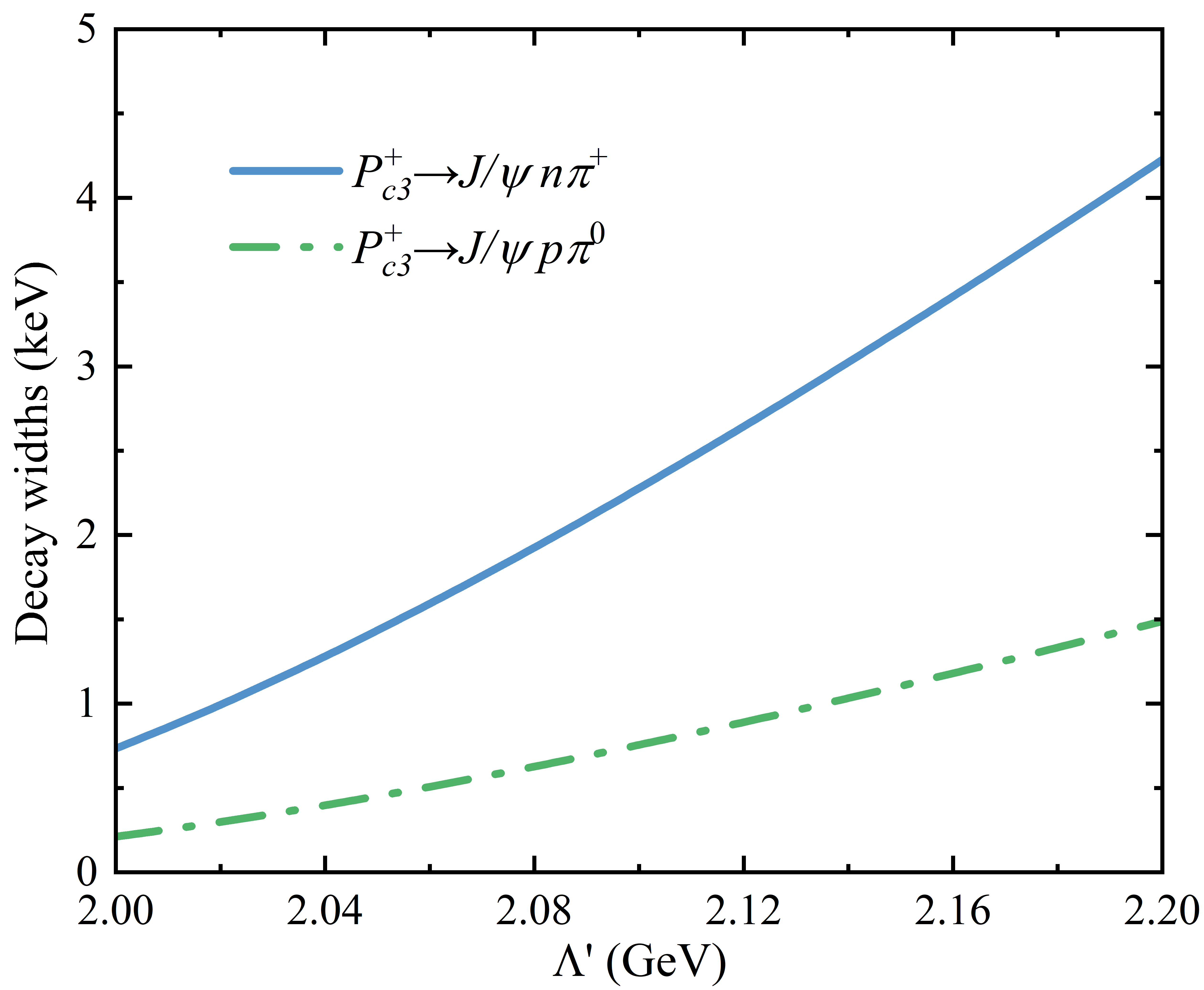
(a)  $P_{c3}$-Scenario A

(b)  $P_{c3}$-Scenario B

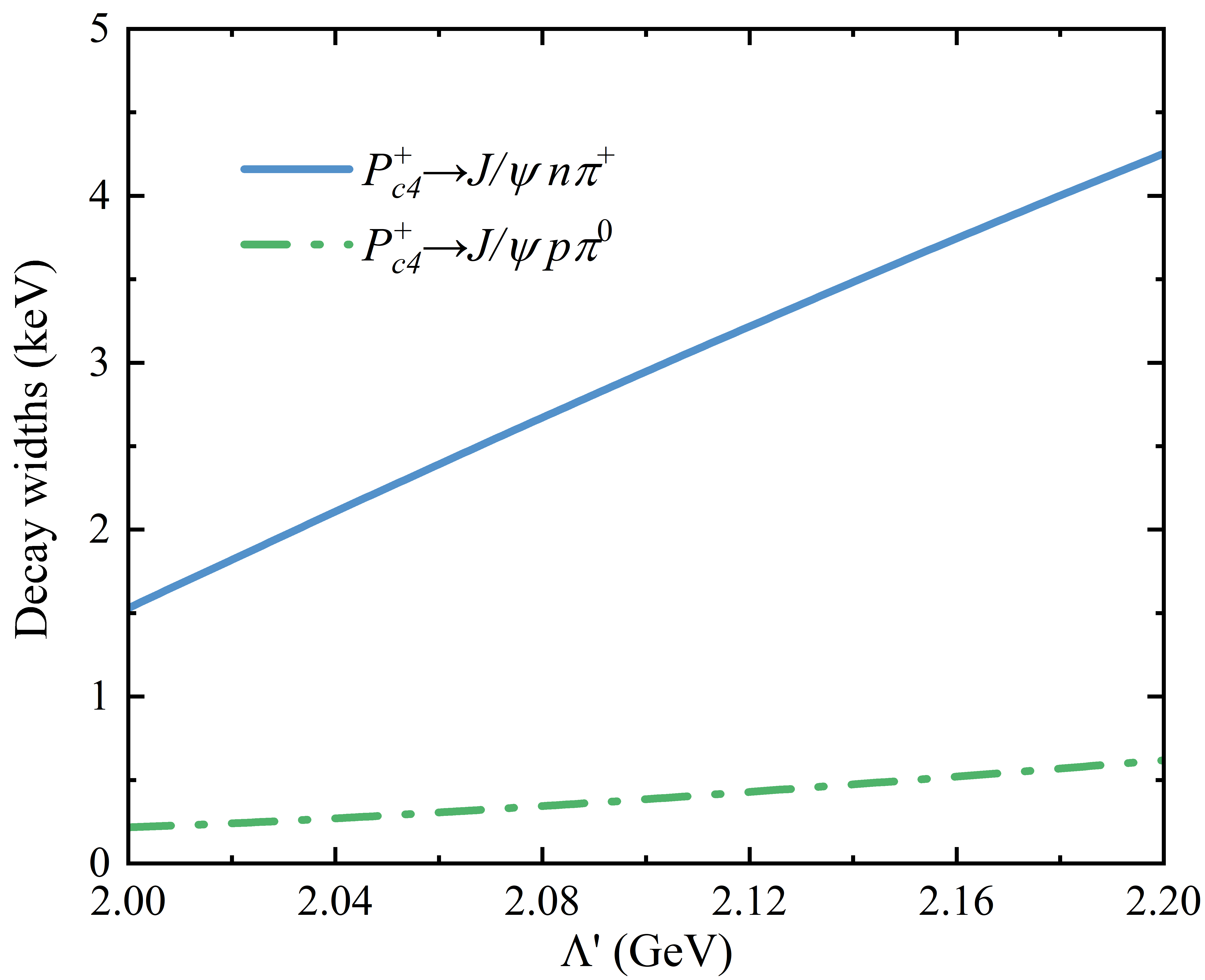
(c)  $P_{c4}$-Scenario A

(d)  $P_{c4}$-Scenario B

Figure 3: Partial decay widths of $P_{c3|c4}^{+}\to J/\psi n\pi^{+}$ and $P_{c3|c4}^{+}\to J/\psi p\pi^{0}$ as a function of the cutoff $\Lambda^{\prime}$ in the form factors (32). The results are represented by the blue solid lines and green dot-dashed lines, respectively, which correspond to the couplings determined for a cutoff $\Lambda=$1.5 GeV.

For the triangle-loop diagrams, we have introduced a form factor in Eq. (32) to suppress the ultraviolate divergence. The parameter $\Lambda^{\prime}$ is usually estimated by the relationship $\Lambda^{\prime}=m_{E}+\alpha\Lambda_{QCD}$, where $m_{E}$ is the mass of the exchanged particle, $\Lambda_{QCD}\sim 200-300$ MeV is the scale parameter of quantum chromodynamics (QCD), and $\alpha$ is a dimensionless parameter of order unity. Following our previous work, we vary $\alpha$ from 0.5 to 1.5 Ling et al. (2021), and then $\Lambda^{\prime}$ varies from 2.0 to 2.2 GeV.

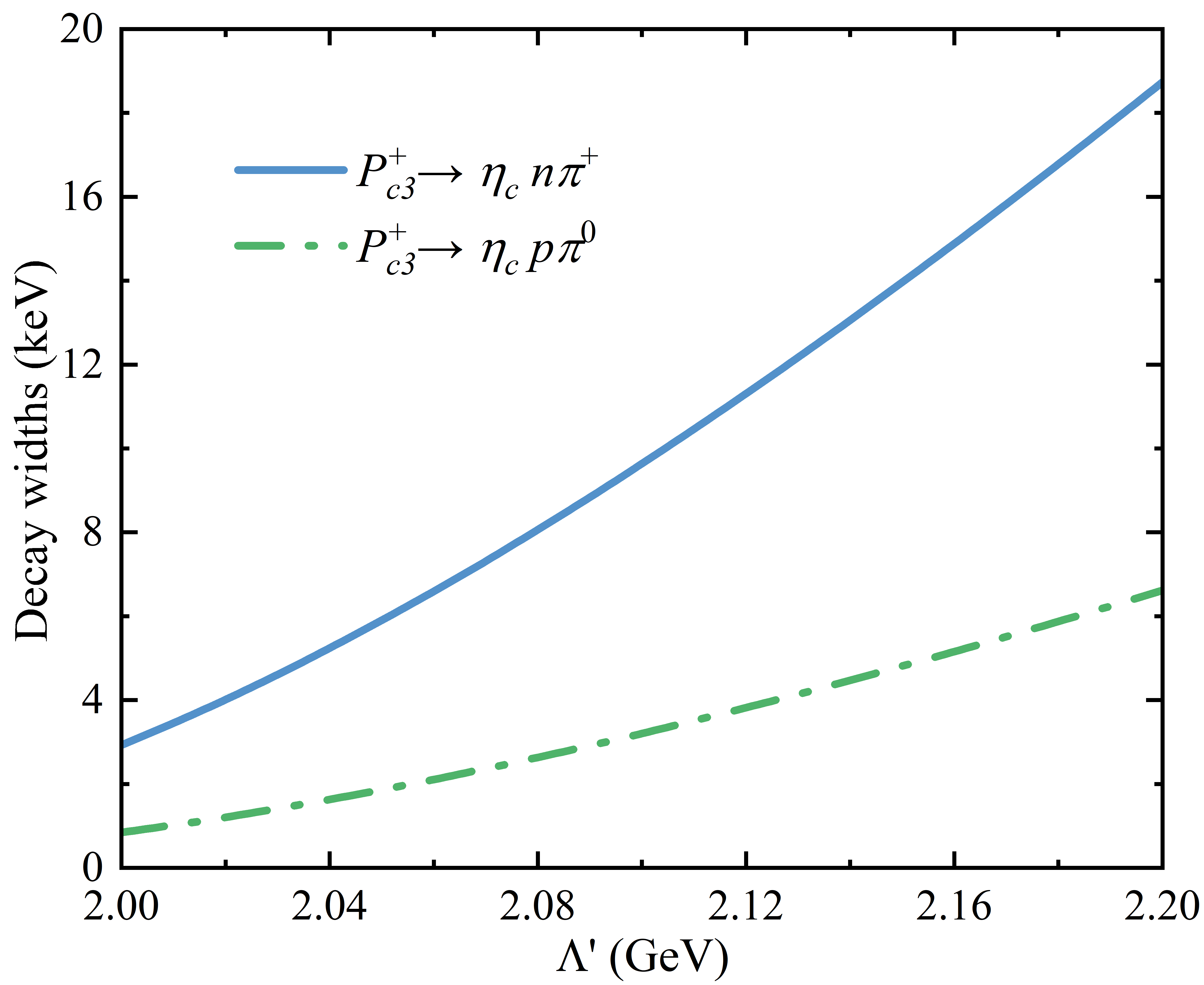
(a)  $P_{c3}$-Scenario A

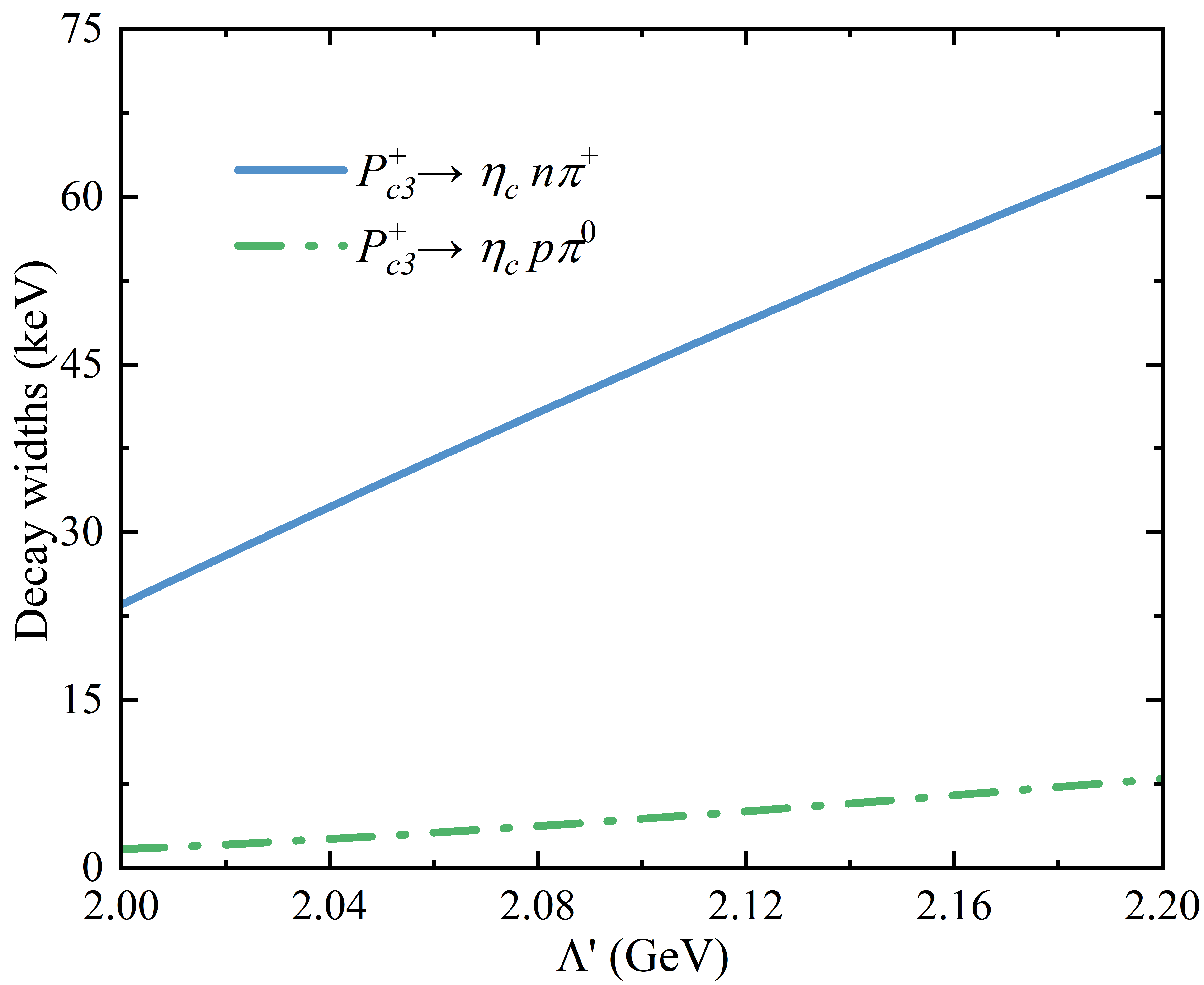
(b)  $P_{c3}$-Scenario B

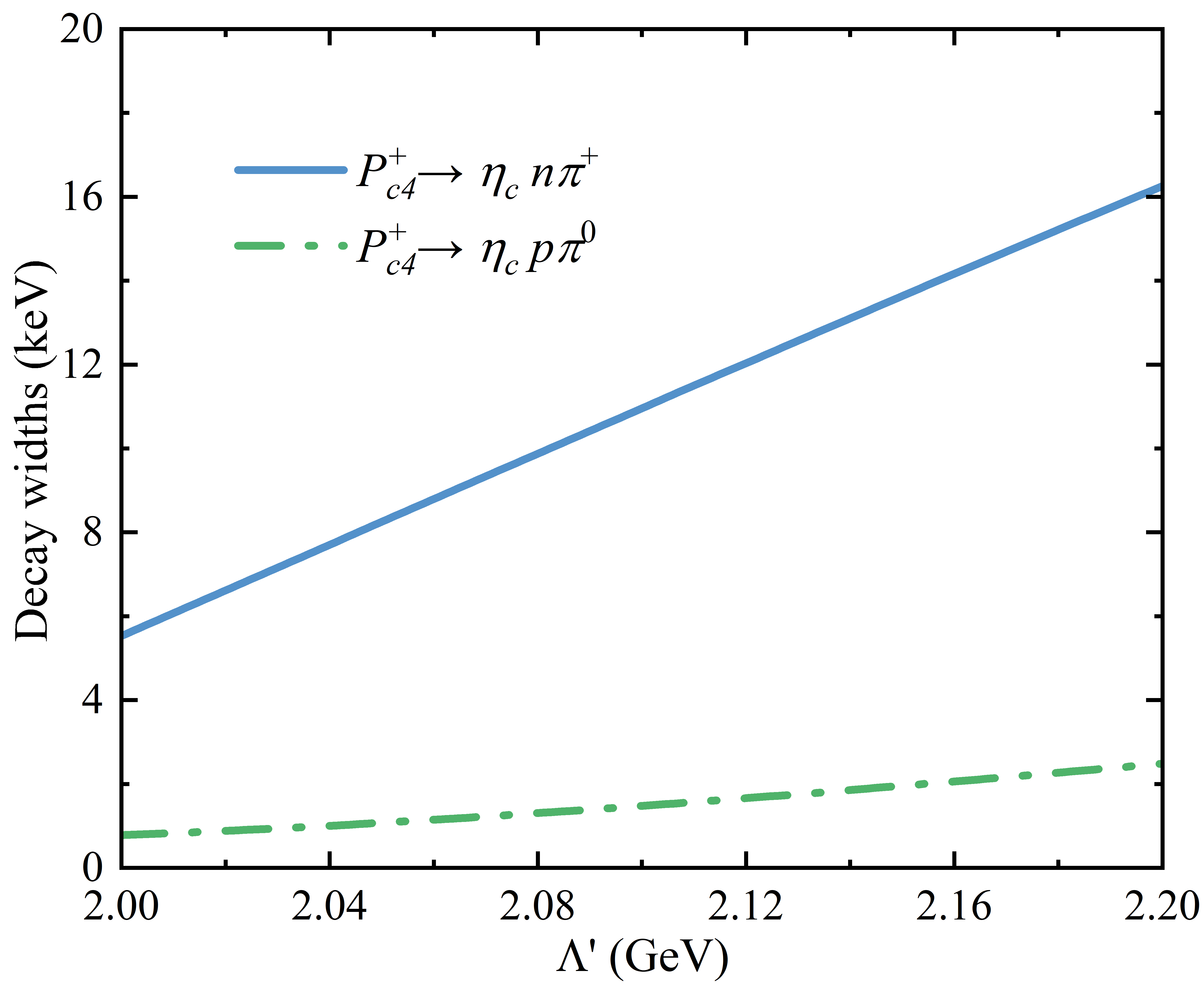
(c)  $P_{c4}$-Scenario A

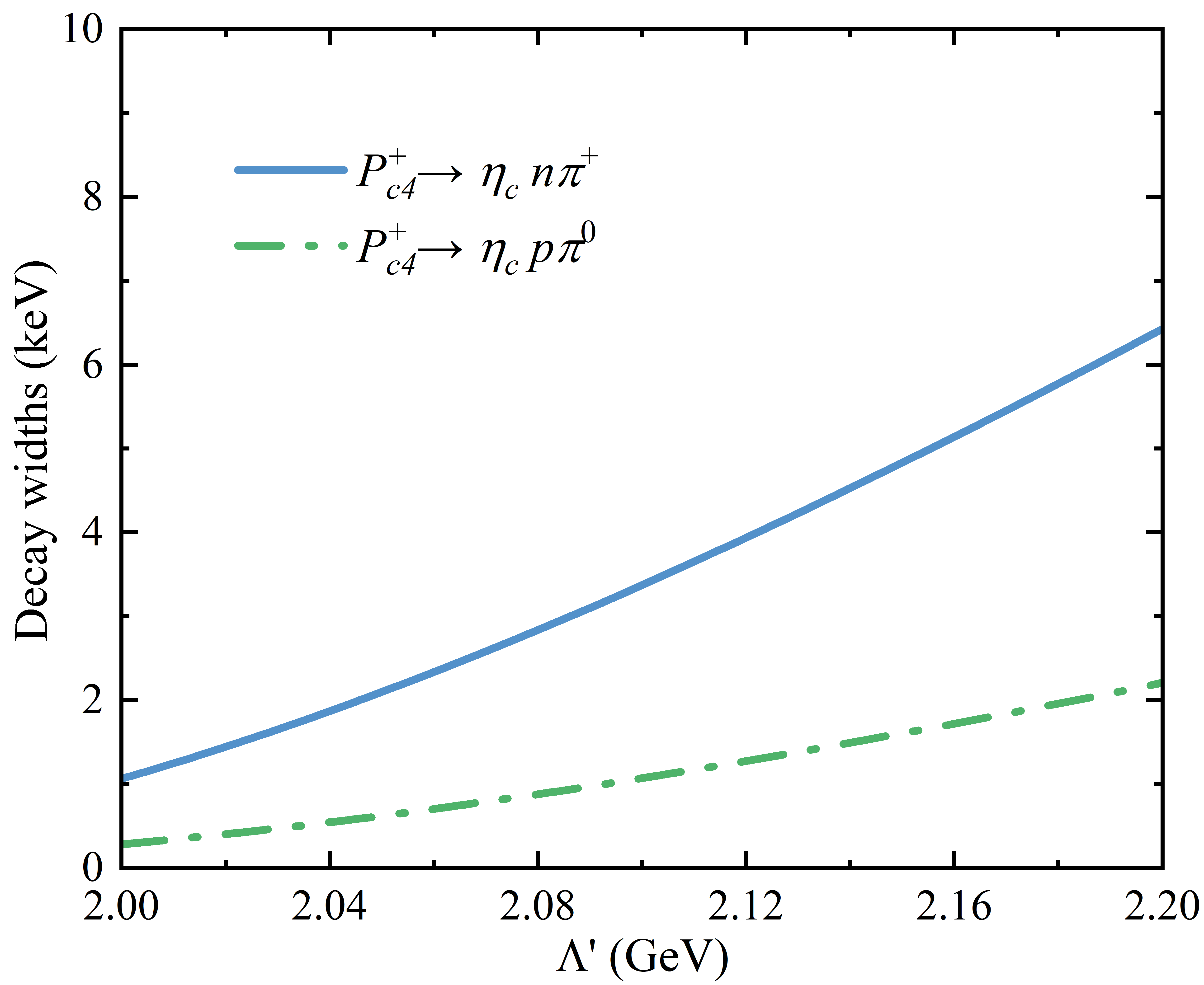
(d)  $P_{c4}$-Scenario B

Figure 4: Partial decay widths of $P_{c3|c4}^{+}\to\eta_{c}n\pi^{+}$ and $P_{c3|c4}^{+}\to\eta_{c}p\pi^{0}$ as a function of the cutoff $\Lambda^{\prime}$ in the form factors (32). The results are represented by the blue solid lines and green dot-dashed lines, respectively, which correspond to the couplings determined for a cutoff $\Lambda=$1.5 GeV.

In Fig. 3, we plot the partial decay widths of $P_{c}(4440)$ and $P_{c}(4457)$ into $J/\psi N\pi$ as a function of the cutoff parameter $\Lambda^{\prime}$. One can see that the widths are only several keV in both Scenario A and B, which are weakly dependent on the variations of both the couplings and the cutoff $\Lambda^{\prime}$. The widths in both scenarios are similar, which indicates that one cannot discriminate the spins of $P_{c}(4440)$ and $P_{c}(4457)$ in the $J/\psi N\pi$ channel, consistent with our previous work Ling et al. (2021). The partial decay width of $P_{c}(4457)$ into $J/\psi N\pi$ account for only 0.1 percent of its total decay width, which is much smaller than that decaying into $\bar{D}\Lambda_{c}\pi$.

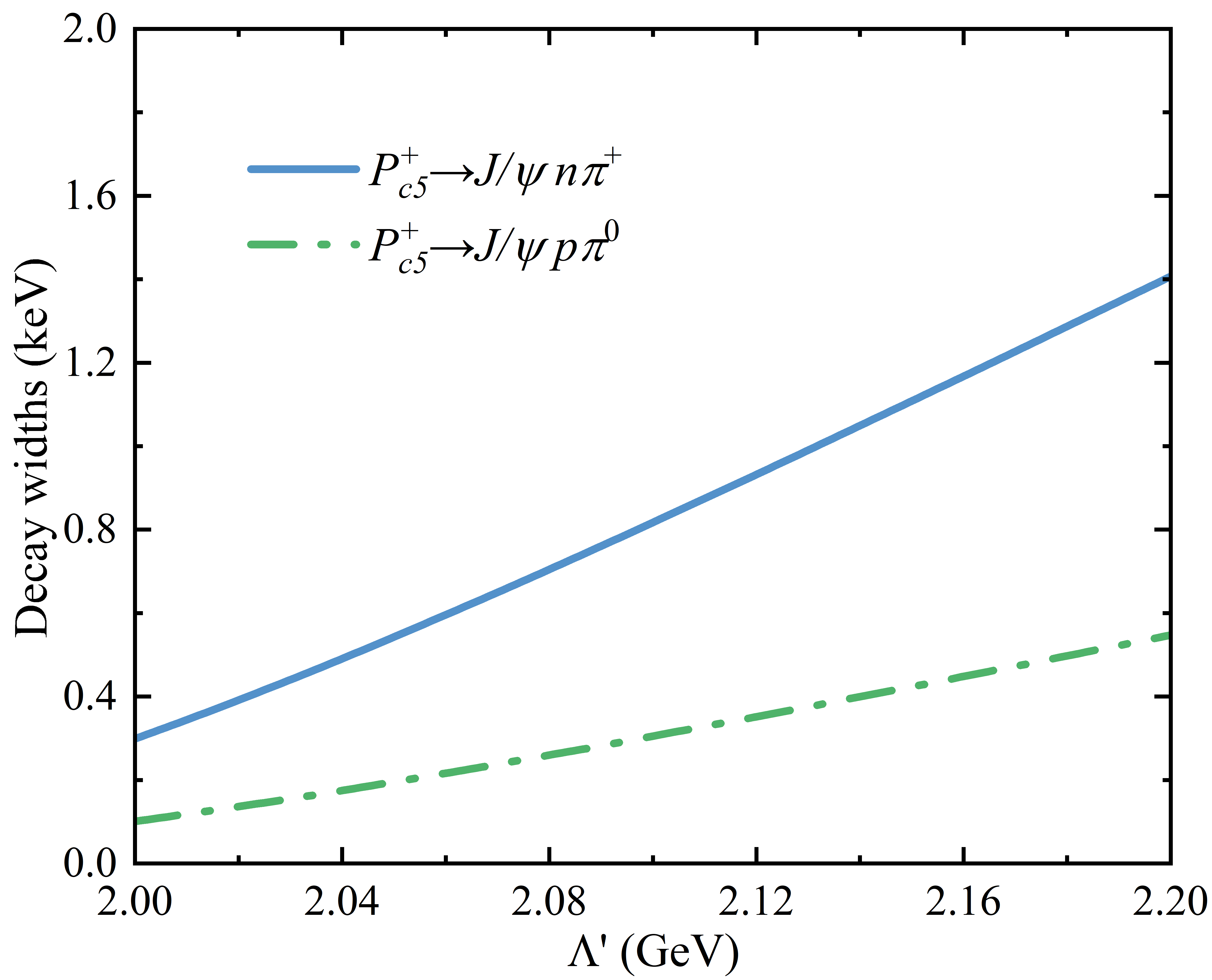
(a)  $P_{c5}$-Scenario A

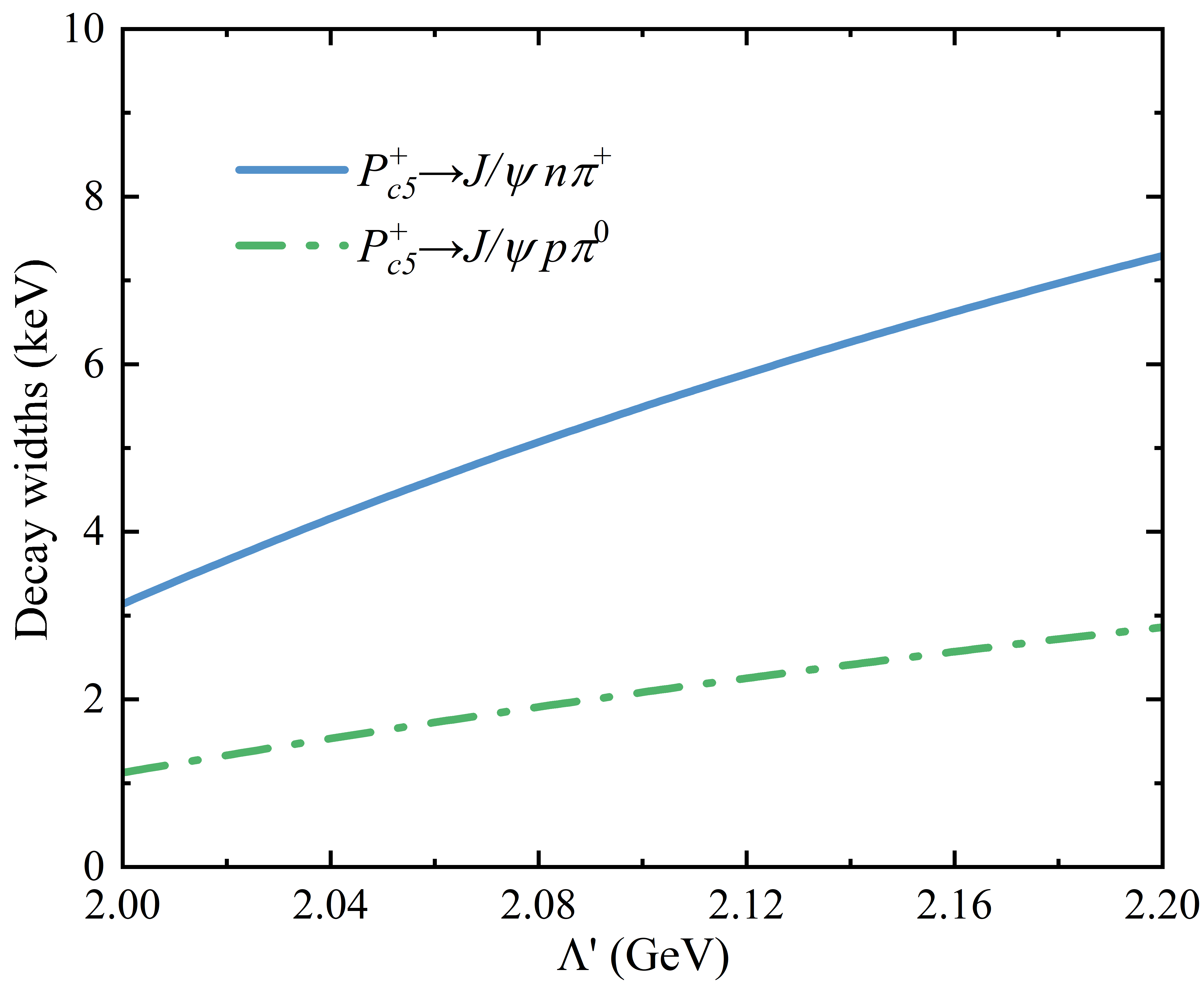
(b)  $P_{c5}$-Scenario B

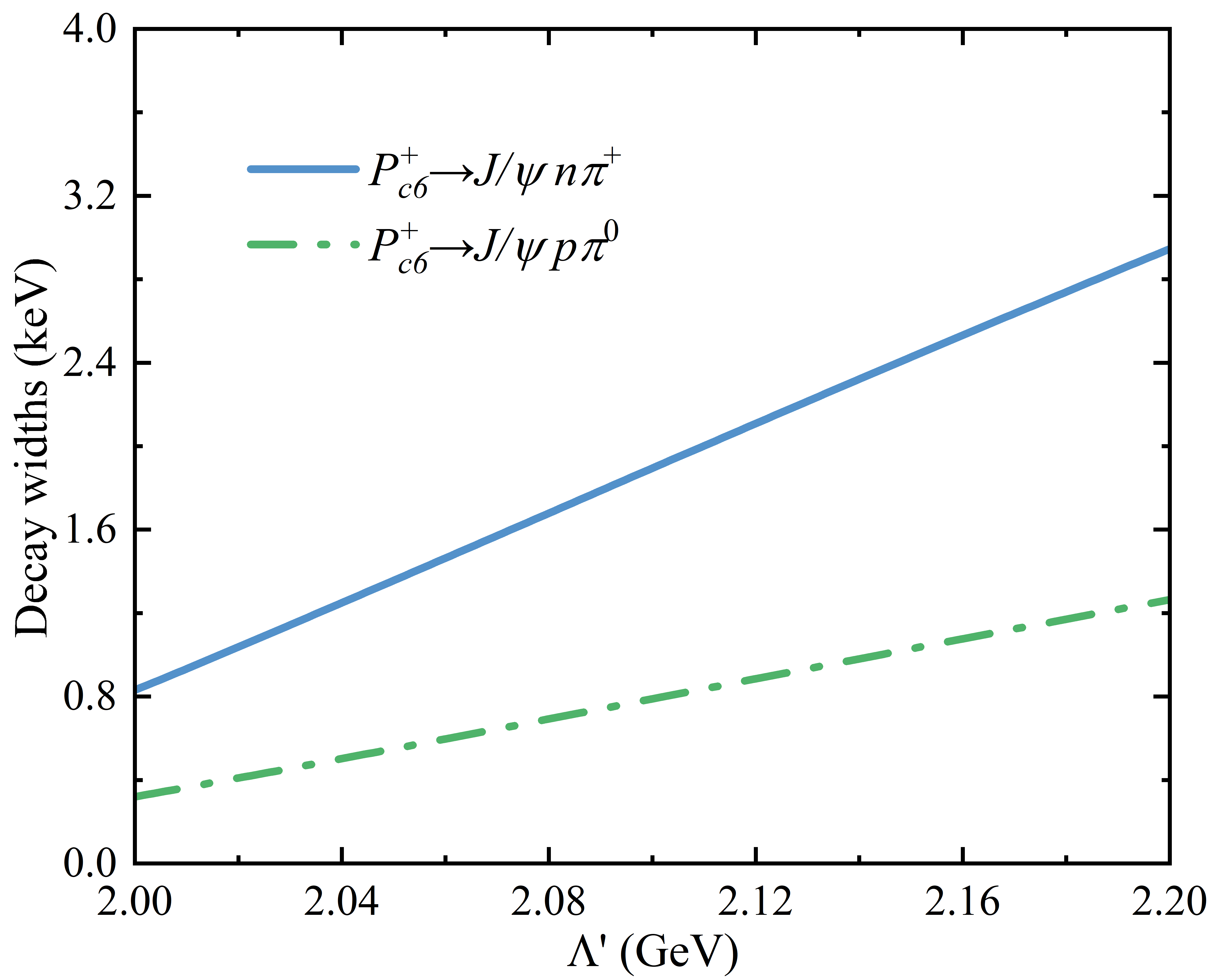
(c)  $P_{c6}$-Scenario A

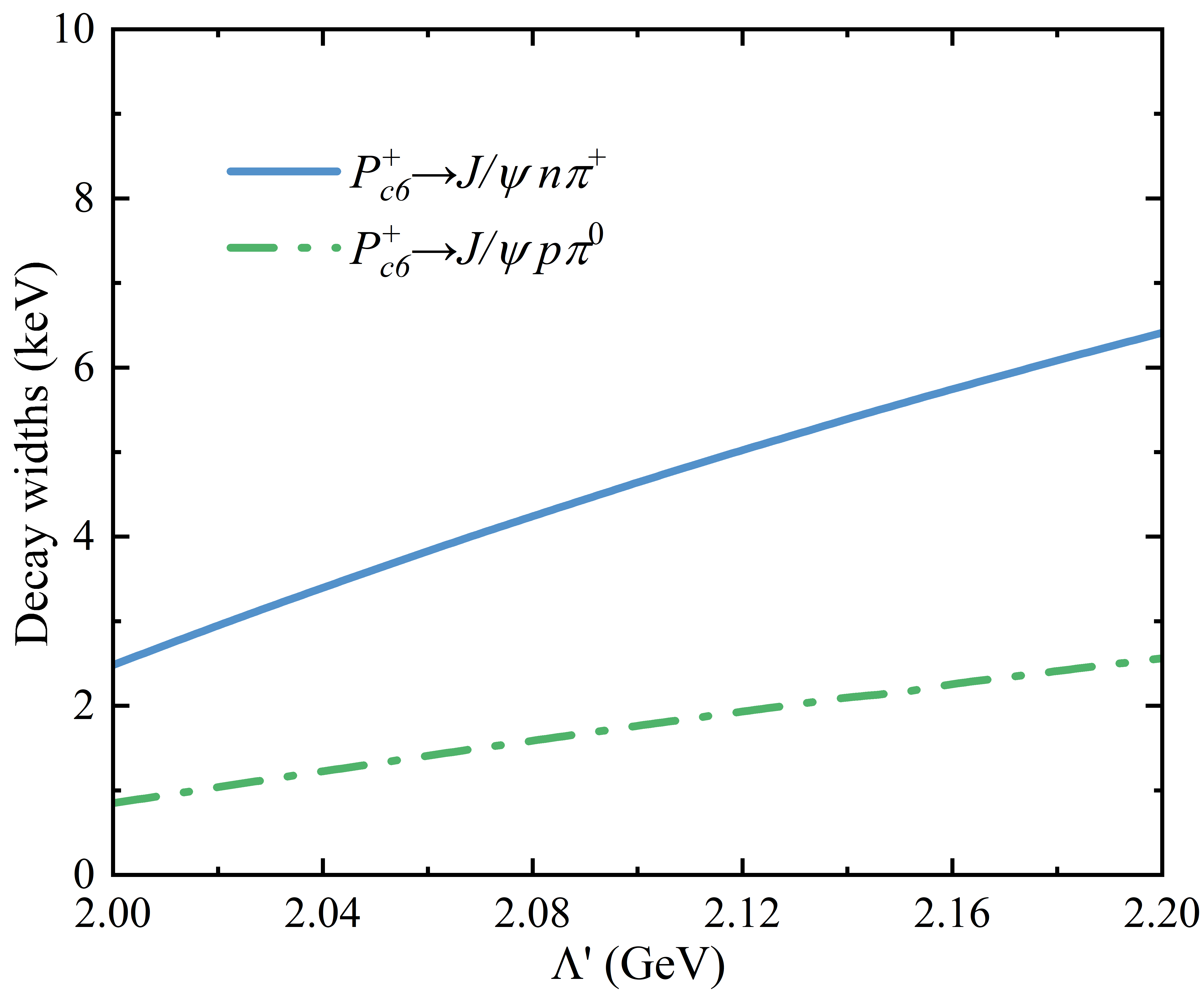
(d)  $P_{c6}$-Scenario B

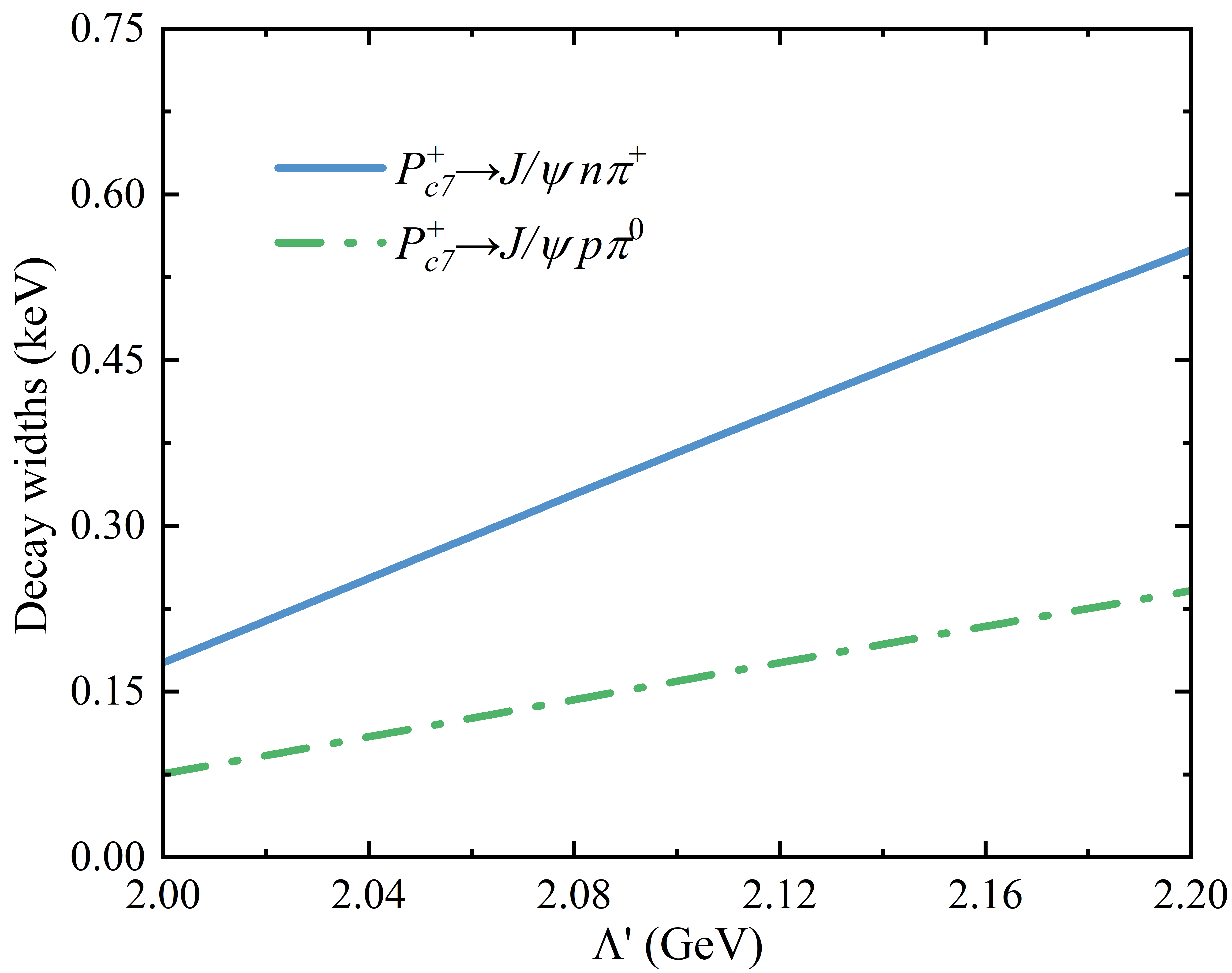
(e)  $P_{c7}$-Scenario A

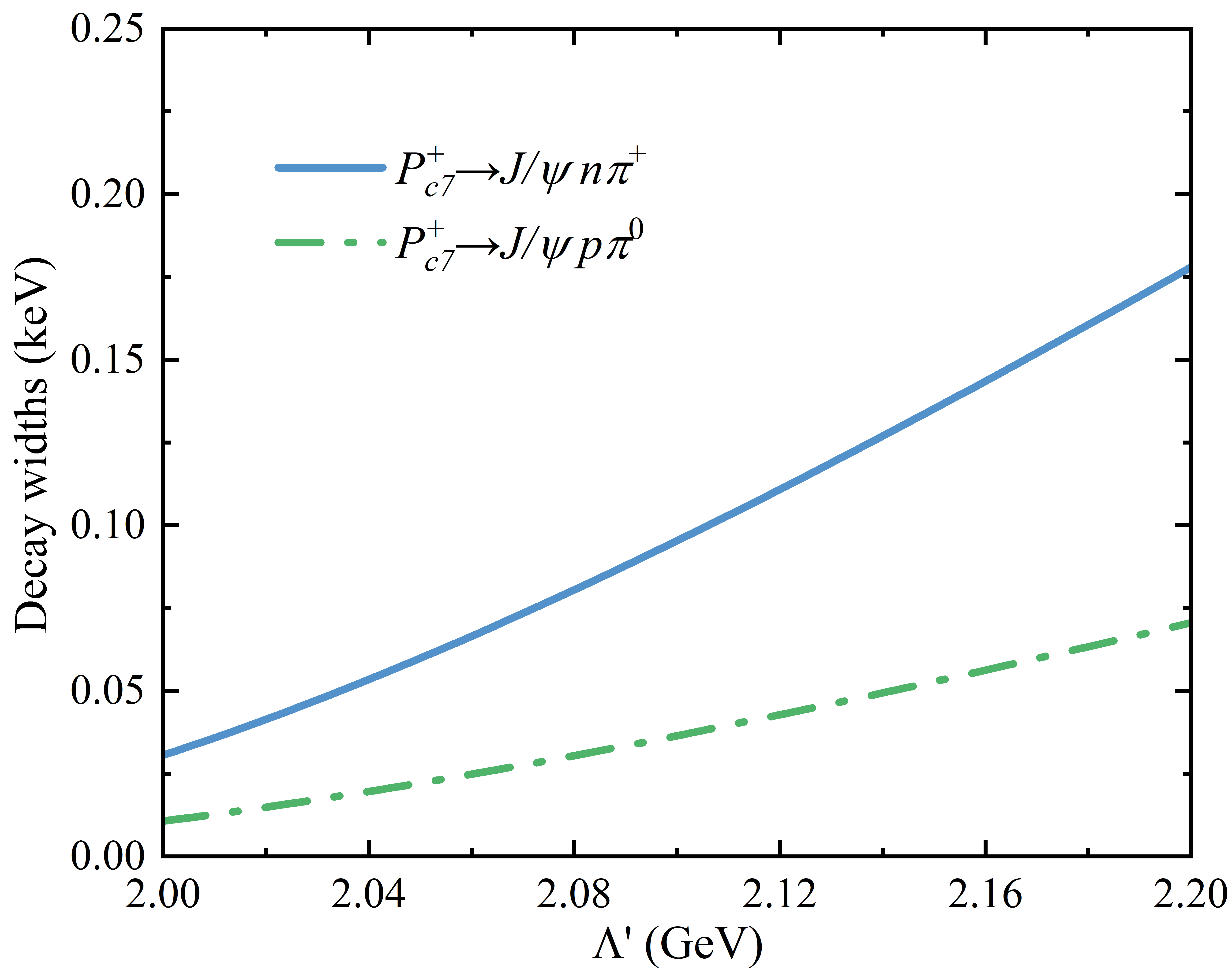
(f)  $P_{c7}$-Scenario B

Figure 5: Partial decay widths of $P_{c5|c6|c7}^{+}\to J/\psi n\pi^{+}$ and $P_{c5|c6|c7}^{+}\to J/\psi p\pi^{0}$ as a function of the cutoff $\Lambda^{\prime}$ of the form factor (32). The results are represented by the blue solid lines and green dot-dashed lines, respectively, which correspond to the couplings determined for a cutoff $\Lambda=$1.5 GeV.

Apart from decaying into $J/\psi N\pi$, $P_{c}(4440)$ and $P_{c}(4457)$ can decay into $\eta_{c}N\pi$ via $\bar{D}\Sigma_{c}$ rescattering to $\eta_{c}N$ if they have $J=1/2$. It is natural to expect that the partial decay widths of $P_{c}(4440)$ and $P_{c}(4457)$ into $\eta_{c}N\pi$ are larger than those into $J/\psi N\pi$ because $P_{c}(4312)$ couples more to $\eta_{c}N$ than to $J/\psi N$. In Fig. 4, we plot the partial decay widths of $P_{c}(4440)$ and $P_{c}(4457)$ into $\eta_{c}N\pi$ as a function of the cutoff parameter $\Lambda^{\prime}$. They are tens of keV, which are much larger than those into $J/\psi N\pi$ in Fig. 3. However, the widths in both Scenario A and B are similar, which also cannot discriminate the spins of $P_{c}(4440)$ and $P_{c}(4457)$. On the other hand, the branching ratios of $P_{c}(4440)$ and $P_{c}(4457)$ decaying into $\eta_{c}N\pi$, $J/\psi N\pi$, and $\bar{D}\Lambda_{c}\pi$ obtained in this work can be used to test the molecular nature of $P_{c}(4440)$ and $P_{c}(4457)$ if these decay channels are detected in future experiments.

We further predict the partial decay widths of $P_{c5}$, $P_{c6}$, and $P_{c7}$ into $J/\psi N\pi$ in the triangle-loop mechanism. In Fig. 5, we plot their widths as a function of the cutoff parameter $\Lambda^{\prime}$. The partial decay widths of $P_{c5}$ and $P_{c6}$ in Scenario B are several keV, while those in Scenario A are at the order of 1 keV. The partial decay widths of $P_{c5}$ in Scenario A and B are more different than those of $P_{c6}$ due to the larger difference in the phase space of $P_{c5}$ into $J/\psi N\pi$ as shown in Table 3 and Table 4, similar to the case of $P_{c3}$. The partial widths of $P_{c7}$ decaying into $J/\psi N\pi$ are less than 1 keV, while the width in Scenario A is larger than that in Scenario B, similar to the case of $P_{c4}$. The partial widths of $P_{c7}$ decaying into $J/\psi N\pi$ are much smaller than those of $P_{c5}$ and $P_{c6}$, which are suppressed by the higher spin of $P_{c7}$, the smaller phase space of $P_{c7}$ decaying into $J/\psi N\pi$ in Scenario B, and the smaller coupling of $P_{c7}$ to $\bar{D}^{\ast}\Sigma_{c}^{\ast}$ in Scenario A.

IV Summary and Discussion

Inspired by the discovery of $T_{cc}$ by the LHCb Collaboration in the $DD\pi$ three-body final state, we adopted the effective Lagrangian approach to systematically study seven $\bar{D}^{(\ast)}\Sigma_{c}^{(\ast)}$ hadronic molecules decaying into three-body final states via two modes, tree level and triangle loop. In the tree-level mode the $\bar{D}^{(\ast)}\Sigma_{c}^{(\ast)}$ molecules decay via subsequent decays of $\Sigma_{c}$ and $\Sigma_{c}^{\ast}$ into $\Lambda_{c}\pi$. In the triangle mode the $\bar{D}^{(\ast)}\Sigma_{c}^{\ast}$ molecules decay into $J/\psi N\pi$ and $\eta_{c}N\pi$ via a two-step process, i.e., first $\bar{D}^{\ast}$ decays into $\bar{D}\pi$, and then $\bar{D}\Sigma_{c}^{(\ast)}$ rescatters into $J/\psi N$ and $\eta_{c}N$. The masses and widths of the $\bar{D}^{(\ast)}\Sigma_{c}^{(\ast)}$ molecules and relevant couplings were determined in the coupled-channel contact-range EFT approach.

Our results show that the partial decay widths of $P_{c2}$, $P_{c}(4457)$, $P_{c5}$, $P_{c6}$ and $P_{c7}$ into $\bar{D}^{(\ast)}\Lambda_{c}\pi$, of the order of several MeV, are much larger than those of $P_{c}(4312)$ and $P_{c}(4440)$, and therefore are more accessible in future experiments. The partial decay widths of $P_{c}(4440)$ and $P_{c}(4457)$ into $J/\psi N\pi$ and $\eta_{c}N\pi$ are only several and tens of keV, respectively, both of which are similar in scenarios A and B. We predicted the partial decay widths of $P_{c5}$, $P_{c6}$, and $P_{c7}$ into $J/\psi N\pi$, among which the width of $P_{c7}\to J/\psi N\pi$ is one order of magnitude smaller than those of $P_{c5}$ and $P_{c6}$. Our results suggest that one should look for $P_{c7}$ in the $J/\psi N\pi$ and $\bar{D}^{\ast}\Lambda_{c}\pi$ invariant mass distributions, while the latter is preferable. These three-body decay modes of the pentaquark states are of great value to further observations of the pentaquark states. In addition, those partial decay widths are helpful to test their molecular nature.

It should be noted that although the predicted partial decay widths of $P_{c2}$, $P_{c5}$, $P_{c6}$, $P_{c7}$ are all dependent on the adopted value for the coupling $g$, our qualitative conclusions should be relatively robust, unless HQSS is broken much strongly than naively anticipated. As a result, the present study of three-body decay modes is expected to stimulate future experimental searches for the known and predicted $\bar{D}^{(*)}\Sigma_{c}^{(*)}$ molecules.

V Acknowledgments

MZL thank Jun-Xu Lu and Ya-Wen Pan for useful discussions. This work is supported in part by the National Natural Science Foundation of China under Grants No.11975041, No.11735003, and No.11961141004. Ming-Zhu Liu acknowledges support from the National Natural Science Foundation of China under Grant No.12105007 and China Postdoctoral Science Foundation under Grants No. 2022M710317, and No. 2022T150036.

Appendix A Invariant amplitudes for the tree-level and triangle-loop processes

The tree-level amplitudes of the $\bar{D}^{(\ast)}\Sigma_{c}^{(\ast)}$ hadronic molecules decaying into $\bar{D}^{(\ast)}\Lambda_{c}\pi$ read

$$\mathcal{M}_{P_{c1}\to\bar{D}\Lambda_{c}\pi} = i\frac{g_{P_{c1}\bar{D}\Sigma_{c}}g_{\Sigma_{c}\Lambda_{c}\pi}}{f_{\pi}}~{}\bar{u}(p_{1}){p\!\!\!/}_{2}\gamma_{5}\frac{1}{{k\!\!\!/}_{1}-m_{\Sigma_{c}}}u(k_{0}),$$ (18)

$$\mathcal{M}_{P_{c2}\to\bar{D}\Lambda_{c}\pi} = i\frac{g_{P_{c2}\bar{D}\Sigma_{c}^{\ast}}g_{\Sigma_{c}^{\ast}\Lambda_{c}\pi}}{f_{\pi}}~{}\bar{u}(p_{1}){p}_{2\mu}\frac{{k\!\!\!/}_{1}+m_{\Sigma_{c}^{\ast}}}{k_{1}^{2}-m_{\Sigma_{c}^{\ast}}^{2}+im_{\Sigma_{c}^{\ast}}\Gamma_{\Sigma_{c}^{\ast}}}P^{\mu\nu}(k_{1})u_{\nu}(k_{0}),$$ (19)

$$\mathcal{M}_{P_{c3}\to\bar{D}^{\ast}\Lambda_{c}\pi} = i\frac{g_{P_{c3}\bar{D}^{\ast}\Sigma_{c}}g_{\Sigma_{c}\Lambda_{c}\pi}}{f_{\pi}}~{}\bar{u}(p_{1}){p\!\!\!/}_{2}\gamma_{5}\frac{1}{{k\!\!\!/}_{1}-m_{\Sigma_{c}}}\widetilde{\gamma}^{\mu}\gamma_{5}\varepsilon_{\mu}(p_{3})u(k_{0}),$$ (20)

$$\mathcal{M}_{P_{c4}\to\bar{D}^{\ast}\Lambda_{c}\pi} = i\frac{g_{P_{c4}\bar{D}^{\ast}\Sigma_{c}}g_{\Sigma_{c}\Lambda_{c}\pi}}{f_{\pi}}~{}\bar{u}(p_{1}){p\!\!\!/}_{2}\gamma_{5}\frac{1}{{k\!\!\!/}_{1}-m_{\Sigma_{c}}}\varepsilon_{\mu}(p_{3})u^{\mu}(k_{0}),$$ (21)

$$\mathcal{M}_{P_{c5}\to\bar{D}^{\ast}\Lambda_{c}\pi} = i\frac{g_{P_{c5}\bar{D}^{\ast}\Sigma_{c}^{\ast}}g_{\Sigma_{c}^{\ast}\Lambda_{c}\pi}}{f_{\pi}}~{}\bar{u}(p_{1})p_{2\mu}\frac{{k\!\!\!/}_{1}+m_{\Sigma_{c}^{\ast}}}{k_{1}^{2}-m_{\Sigma_{c}^{\ast}}^{2}+im_{\Sigma_{c}^{\ast}}\Gamma_{\Sigma_{c}^{\ast}}}P^{\mu\nu}(k_{1})\varepsilon_{\nu}(p_{3})u(k_{0}),$$ (22)

$$\mathcal{M}_{P_{c6}\to\bar{D}^{\ast}\Lambda_{c}\pi} = i\frac{g_{P_{c6}\bar{D}^{\ast}\Sigma_{c}^{\ast}}g_{\Sigma_{c}^{\ast}\Lambda_{c}\pi}}{f_{\pi}}~{}\bar{u}(p_{1})p_{2\mu}\frac{{k\!\!\!/}_{1}+m_{\Sigma_{c}^{\ast}}}{k_{1}^{2}-m_{\Sigma_{c}^{\ast}}^{2}+im_{\Sigma_{c}^{\ast}}\Gamma_{\Sigma_{c}^{\ast}}}P^{\mu\nu}(k_{1})\varepsilon_{\rho}(p_{3})\gamma_{5}\widetilde{\gamma}^{\rho}u_{\nu}(k_{0}),$$ (23)

$$\mathcal{M}_{P_{c7}\to\bar{D}^{\ast}\Lambda_{c}\pi} = i\frac{g_{P_{c7}\bar{D}^{\ast}\Sigma_{c}^{\ast}}g_{\Sigma_{c}^{\ast}\Lambda_{c}\pi}}{f_{\pi}}~{}\bar{u}(p_{1})p_{2\mu}\frac{{k\!\!\!/}_{1}+m_{\Sigma_{c}^{\ast}}}{k_{1}^{2}-m_{\Sigma_{c}^{\ast}}^{2}+im_{\Sigma_{c}^{\ast}}\Gamma_{\Sigma_{c}^{\ast}}}P^{\mu\nu}(k_{1})\varepsilon_{\rho}(p_{3}){u_{\nu}}^{\rho}(k_{0}),$$ (24)

where $k_{0}$ and $k_{1}$ denote the momenta of initial states and intermediate states, and the momenta of $\Lambda_{c}$, $\pi$, and $\bar{D}^{(\ast)}$ are represented by $p_{1}$, $p_{2}$, and $p_{3}$, respectively. $\bar{u}(p_{1})$ and $u(k_{0})$ denote the final and initial spinor wave functions, respectively. $P^{\mu\nu}(p)=g^{\mu\nu}-\frac{1}{3}\gamma^{\mu}\gamma^{\nu}-\frac{\gamma^{\nu}p^{\mu}-\gamma^{\mu}p^{\nu}}{3m}-\frac{2p^{\mu}p^{\nu}}{3m^{2}}$ denotes the propagator of a massive particle of spin $3/2$.

The amplitudes of the $\bar{D}^{\ast}\Sigma_{c}$ molecules decaying into $\eta_{c}N\pi$ read

$$i\mathcal{M}_{1/2} = g_{P_{c3}\bar{D}^{\ast}\Sigma_{c}}g_{D^{\ast}D\pi}\int\frac{d^{4}q}{(2\pi)^{4}}\bar{u}(p_{1})T_{\bar{D}\Sigma_{c}\to\eta_{c}N}(\sqrt{s})\frac{1}{{/\!\!\!k}_{1}-m_{\Sigma_{c}}}$$ (25)

$$\frac{1}{q^{2}-m_{\bar{D}}^{2}}p_{3\alpha}\frac{-g^{\alpha\beta}+\frac{k_{2}^{\alpha}k_{2}^{\beta}}{m_{\bar{D}^{\ast}}^{2}}}{k_{2}^{2}-m_{\bar{D}^{\ast}}^{2}}\widetilde{\gamma}_{\beta}\gamma_{5}u(k_{0})F(q^{2}),$$

$$i\mathcal{M}_{3/2} = g_{P_{c4}\bar{D}^{\ast}\Sigma_{c}}g_{D^{\ast}D\pi}\int\frac{d^{4}q}{(2\pi)^{4}}\bar{u}(p_{1})T_{\bar{D}\Sigma_{c}\to\eta_{c}N}(\sqrt{s})\frac{1}{{/\!\!\!k}_{1}-m_{\Sigma_{c}}}$$ (26)

$$\frac{1}{q^{2}-m_{\bar{D}}^{2}}p_{3\alpha}\frac{-g^{\alpha\beta}+\frac{k_{2}^{\alpha}k_{2}^{\beta}}{m_{\bar{D}^{\ast}}^{2}}}{k_{2}^{2}-m_{\bar{D}^{\ast}}^{2}}u_{\beta}(k_{0})F(q^{2}),$$

and the amplitudes of the $\bar{D}^{\ast}\Sigma_{c}^{(\ast)}$ molecules decaying into $J/\psi N\pi$ read

$$i\mathcal{M}_{1/2} = g_{P_{c3}\bar{D}^{\ast}\Sigma_{c}}g_{D^{\ast}D\pi}\int\frac{d^{4}q}{(2\pi)^{4}}\bar{u}(p_{1})\varepsilon_{\mu}(p_{2})\gamma^{\mu}\gamma_{5}T_{\bar{D}\Sigma_{c}\to J/\psi N}(\sqrt{s})\frac{1}{{/\!\!\!k}_{1}-m_{\Sigma_{c}}}$$ (27)

$$\frac{1}{q^{2}-m_{\bar{D}}^{2}}p_{3\alpha}\frac{-g^{\alpha\beta}+\frac{k_{2}^{\alpha}k_{2}^{\beta}}{m_{\bar{D}^{\ast}}^{2}}}{k_{2}^{2}-m_{\bar{D}^{\ast}}^{2}}\widetilde{\gamma}_{\beta}\gamma_{5}u(k_{0})F(q^{2}),$$

$$i\mathcal{M}_{3/2} = g_{P_{c4}\bar{D}^{\ast}\Sigma_{c}}g_{D^{\ast}D\pi}\int\frac{d^{4}q}{(2\pi)^{4}}\bar{u}(p_{1})\varepsilon_{\mu}(p_{2})\gamma^{\mu}\gamma_{5}T_{\bar{D}\Sigma_{c}\to J/\psi N}(\sqrt{s})\frac{1}{{/\!\!\!k}_{1}-m_{\Sigma_{c}}}$$ (28)

$$\frac{1}{q^{2}-m_{\bar{D}}^{2}}p_{3\alpha}\frac{-g^{\alpha\beta}+\frac{k_{2}^{\alpha}k_{2}^{\beta}}{m_{\bar{D}^{\ast}}^{2}}}{k_{2}^{2}-m_{\bar{D}^{\ast}}^{2}}u_{\beta}(k_{0})F(q^{2}),$$

$$i\mathcal{M}_{1/2} = g_{P_{c5}\bar{D}^{\ast}\Sigma_{c}^{\ast}}g_{D^{\ast}D\pi}\int\frac{d^{4}q}{(2\pi)^{4}}\bar{u}(p_{1})T_{\bar{D}\Sigma_{c}^{\ast}\to J/\psi N}(\sqrt{s})\varepsilon_{\nu}(p_{2})$$ (29)

$$\frac{{k\!\!\!/}_{1}+m_{\Sigma_{c}^{\ast}}}{k_{1}^{2}-m_{\Sigma_{c}^{\ast}}^{2}+im_{\Sigma_{c}^{\ast}}\Gamma_{\Sigma_{c}^{\ast}}}{P^{\nu}}_{\beta}(k_{1})\frac{1}{q^{2}-m_{\bar{D}}^{2}}p_{3\alpha}\frac{-g^{\alpha\beta}+\frac{k_{2}^{\alpha}k_{2}^{\beta}}{m_{\bar{D}^{\ast}}^{2}}}{k_{2}^{2}-m_{\bar{D}^{\ast}}^{2}}u(k_{0})F(q^{2}),$$

$$i\mathcal{M}_{3/2} = g_{P_{c6}\bar{D}^{\ast}\Sigma_{c}^{\ast}}g_{D^{\ast}D\pi}\int\frac{d^{4}q}{(2\pi)^{4}}\bar{u}(p_{1})T_{\bar{D}\Sigma_{c}^{\ast}\to J/\psi N}(\sqrt{s})\varepsilon_{\nu}(p_{2})$$ (30)

$$\frac{{k\!\!\!/}_{1}+m_{\Sigma_{c}^{\ast}}}{k_{1}^{2}-m_{\Sigma_{c}^{\ast}}^{2}+im_{\Sigma_{c}^{\ast}}\Gamma_{\Sigma_{c}^{\ast}}}P^{\nu\rho}(k_{1})\frac{1}{q^{2}-m_{\bar{D}}^{2}}p_{3\alpha}\frac{-g^{\alpha\beta}+\frac{k_{2}^{\alpha}k_{2}^{\beta}}{m_{\bar{D}^{\ast}}^{2}}}{k_{2}^{2}-m_{\bar{D}^{\ast}}^{2}}\gamma_{5}\widetilde{\gamma}_{\beta}u_{\rho}(k_{0})F(q^{2}),$$

$$i\mathcal{M}_{5/2} = g_{P_{c7}\bar{D}^{\ast}\Sigma_{c}^{\ast}}g_{D^{\ast}D\pi}\int\frac{d^{4}q}{(2\pi)^{4}}\bar{u}(p_{1})T_{\bar{D}\Sigma_{c}^{\ast}\to J/\psi N}(\sqrt{s})\varepsilon_{\nu}(p_{2})$$ (31)

$$\frac{{k\!\!\!/}_{1}+m_{\Sigma_{c}^{\ast}}}{k_{1}^{2}-m_{\Sigma_{c}^{\ast}}^{2}+im_{\Sigma_{c}^{\ast}}\Gamma_{\Sigma_{c}^{\ast}}}P^{\nu\rho}(k_{1})\frac{1}{q^{2}-m_{\bar{D}}^{2}}p_{3\alpha}\frac{-g^{\alpha\beta}+\frac{k_{2}^{\alpha}k_{2}^{\beta}}{m_{\bar{D}^{\ast}}^{2}}}{k_{2}^{2}-m_{\bar{D}^{\ast}}^{2}}u_{\beta\rho}(k_{0})F(q^{2}),$$

where $q$, $k_{0}$, $k_{1}$, $k_{2}$, $p_{1}$, $p_{2}$ and $p_{3}$ represent the momenta of $\bar{D}$, $P_{c}$, $\Sigma_{c}^{(\ast)}$, $\bar{D}^{\ast}$, $N$, $J/\psi(\eta_{c})$ and $\pi$, respectively, and $T_{\bar{D}\Sigma_{c}^{(\ast)}-J/\psi(\eta_{c})N}$ represent the potentials of inelastic scattering. To avoid the divergence induced by the loop function, we have introduced a form factor of the form

$$F(q^{2})=\left(\frac{\Lambda^{\prime 2}-m_{\bar{D}}^{2}}{\Lambda^{\prime 2}-q^{2}}\right)^{2}.$$ (32)

References

- Wu et al. (2010) J.-J. Wu, R. Molina, E. Oset, and B. S. Zou, Phys. Rev. Lett. 105, 232001 (2010), arXiv:1007.0573 [nucl-th] .
- Wu et al. (2011) J.-J. Wu, R. Molina, E. Oset, and B. S. Zou, Phys. Rev. C84, 015202 (2011), arXiv:1011.2399 [nucl-th] .
- Wang et al. (2011) W. L. Wang, F. Huang, Z. Y. Zhang, and B. S. Zou, Phys. Rev. C 84, 015203 (2011), arXiv:1101.0453 [nucl-th] .
- Yang et al. (2012) Z.-C. Yang, Z.-F. Sun, J. He, X. Liu, and S.-L. Zhu, Chin. Phys. C 36, 6 (2012), arXiv:1105.2901 [hep-ph] .
- Yuan et al. (2012) S. G. Yuan, K. W. Wei, J. He, H. S. Xu, and B. S. Zou, Eur. Phys. J. A 48, 61 (2012), arXiv:1201.0807 [nucl-th] .
- Wu et al. (2012) J.-J. Wu, T. S. H. Lee, and B. S. Zou, Phys. Rev. C 85, 044002 (2012), arXiv:1202.1036 [nucl-th] .
- Garcia-Recio et al. (2013) C. Garcia-Recio, J. Nieves, O. Romanets, L. L. Salcedo, and L. Tolos, Phys. Rev. D 87, 074034 (2013), arXiv:1302.6938 [hep-ph] .
- Xiao et al. (2013) C. W. Xiao, J. Nieves, and E. Oset, Phys. Rev. D88, 056012 (2013), arXiv:1304.5368 [hep-ph] .
- Uchino et al. (2016) T. Uchino, W.-H. Liang, and E. Oset, Eur. Phys. J. A 52, 43 (2016), arXiv:1504.05726 [hep-ph] .
- Karliner and Rosner (2015) M. Karliner and J. L. Rosner, Phys. Rev. Lett. 115, 122001 (2015), arXiv:1506.06386 [hep-ph] .
- Aaij et al. (2015) R. Aaij et al. (LHCb), Phys. Rev. Lett. 115, 072001 (2015), arXiv:1507.03414 [hep-ex] .
- Aaij et al. (2019a) R. Aaij et al. (LHCb), Phys. Rev. Lett. 122, 222001 (2019a), arXiv:1904.03947 [hep-ex] .
- Aaij et al. (2021) R. Aaij et al. (LHCb), Sci. Bull. 66, 1278 (2021), arXiv:2012.10380 [hep-ex] .
- Aaij et al. (2022a) R. Aaij et al. (LHCb), Phys. Rev. Lett. 128, 062001 (2022a), arXiv:2108.04720 [hep-ex] .
- Chen et al. (2016) H.-X. Chen, L.-S. Geng, W.-H. Liang, E. Oset, E. Wang, and J.-J. Xie, Phys. Rev. C 93, 065203 (2016), arXiv:1510.01803 [hep-ph] .
- Chen et al. (2017) R. Chen, J. He, and X. Liu, Chin. Phys. C 41, 103105 (2017), arXiv:1609.03235 [hep-ph] .
- Shen et al. (2019) C.-W. Shen, J.-J. Wu, and B.-S. Zou, Phys. Rev. D 100, 056006 (2019), arXiv:1906.03896 [hep-ph] .
- Xiao et al. (2019a) C. Xiao, J. Nieves, and E. Oset, Phys. Lett. B 799, 135051 (2019a), arXiv:1906.09010 [hep-ph] .
- Wang et al. (2020a) B. Wang, L. Meng, and S.-L. Zhu, Phys. Rev. D 101, 034018 (2020a), arXiv:1912.12592 [hep-ph] .
- Yan et al. (2022) M.-J. Yan, F.-Z. Peng, M. Sánchez Sánchez, and M. Pavon Valderrama, Eur. Phys. J. C 82, 574 (2022), arXiv:2108.05306 [hep-ph] .
- Deng (2022) C.-R. Deng, Phys. Rev. D 105, 116021 (2022), arXiv:2202.13570 [hep-ph] .
- Nakamura et al. (2021) S. X. Nakamura, A. Hosaka, and Y. Yamaguchi, Phys. Rev. D 104, L091503 (2021), arXiv:2109.15235 [hep-ph] .
- Wang et al. (2021) J.-Z. Wang, X. Liu, and T. Matsuki, Phys. Rev. D 104, 114020 (2021), arXiv:2110.09423 [hep-ph] .
- Liu et al. (2019) M.-Z. Liu, Y.-W. Pan, F.-Z. Peng, M. Sánchez Sánchez, L.-S. Geng, A. Hosaka, and M. Pavon Valderrama, Phys. Rev. Lett. 122, 242001 (2019), arXiv:1903.11560 [hep-ph] .
- Liu et al. (2021) M.-Z. Liu, T.-W. Wu, M. Sánchez Sánchez, M. P. Valderrama, L.-S. Geng, and J.-J. Xie, Phys. Rev. D 103, 054004 (2021), arXiv:1907.06093 [hep-ph] .
- Chen et al. (2019a) R. Chen, Z.-F. Sun, X. Liu, and S.-L. Zhu, Phys. Rev. D100, 011502 (2019a), arXiv:1903.11013 [hep-ph] .
- He (2019) J. He, Eur. Phys. J. C79, 393 (2019), arXiv:1903.11872 [hep-ph] .
- Chen et al. (2019b) H.-X. Chen, W. Chen, and S.-L. Zhu, Phys. Rev. D100, 051501 (2019b), arXiv:1903.11001 [hep-ph] .
- Xiao et al. (2019b) C. W. Xiao, J. Nieves, and E. Oset, Phys. Rev. D100, 014021 (2019b), arXiv:1904.01296 [hep-ph] .
- Yamaguchi et al. (2020) Y. Yamaguchi, H. García-Tecocoatzi, A. Giachino, A. Hosaka, E. Santopinto, S. Takeuchi, and M. Takizawa, Phys. Rev. D 101, 091502 (2020), arXiv:1907.04684 [hep-ph] .
- Pavon Valderrama (2019) M. Pavon Valderrama, Phys. Rev. D100, 094028 (2019), arXiv:1907.05294 [hep-ph] .
- Du et al. (2020) M.-L. Du, V. Baru, F.-K. Guo, C. Hanhart, U.-G. Meißner, J. A. Oller, and Q. Wang, Phys. Rev. Lett. 124, 072001 (2020), arXiv:1910.11846 [hep-ph] .
- He and Chen (2019) J. He and D.-Y. Chen, Eur. Phys. J. C79, 887 (2019), arXiv:1909.05681 [hep-ph] .
- Wang et al. (2020b) G.-J. Wang, L.-Y. Xiao, R. Chen, X.-H. Liu, X. Liu, and S.-L. Zhu, Phys. Rev. D 102, 036012 (2020b), arXiv:1911.09613 [hep-ph] .
- Burns and Swanson (2019) T. J. Burns and E. S. Swanson, Phys. Rev. D 100, 114033 (2019), arXiv:1908.03528 [hep-ph] .
- Peng et al. (2021a) F.-Z. Peng, J.-X. Lu, M. Sánchez Sánchez, M.-J. Yan, and M. Pavon Valderrama, Phys. Rev. D 103, 014023 (2021a), arXiv:2007.01198 [hep-ph] .
- Yalikun et al. (2021) N. Yalikun, Y.-H. Lin, F.-K. Guo, Y. Kamiya, and B.-S. Zou, Phys. Rev. D 104, 094039 (2021), arXiv:2109.03504 [hep-ph] .
- Xiao et al. (2019c) C.-J. Xiao, Y. Huang, Y.-B. Dong, L.-S. Geng, and D.-Y. Chen, Phys. Rev. D 100, 014022 (2019c), arXiv:1904.00872 [hep-ph] .
- Lin and Zou (2019) Y.-H. Lin and B.-S. Zou, Phys. Rev. D100, 056005 (2019), arXiv:1908.05309 [hep-ph] .
- Wu and Chen (2019) Q. Wu and D.-Y. Chen, Phys. Rev. D100, 114002 (2019), arXiv:1906.02480 [hep-ph] .
- Eides et al. (2020) M. I. Eides, V. Y. Petrov, and M. V. Polyakov, Mod. Phys. Lett. A 35, 2050151 (2020), arXiv:1904.11616 [hep-ph] .
- Ali and Parkhomenko (2019) A. Ali and A. Y. Parkhomenko, Phys. Lett. B 793, 365 (2019), arXiv:1904.00446 [hep-ph] .
- Mutuk (2019) H. Mutuk, Chin. Phys. C 43, 093103 (2019), arXiv:1904.09756 [hep-ph] .
- Wang (2020) Z.-G. Wang, Int. J. Mod. Phys. A 35, 2050003 (2020), arXiv:1905.02892 [hep-ph] .
- Cheng and Liu (2019) J.-B. Cheng and Y.-R. Liu, Phys. Rev. D100, 054002 (2019), arXiv:1905.08605 [hep-ph] .
- Weng et al. (2019) X.-Z. Weng, X.-L. Chen, W.-Z. Deng, and S.-L. Zhu, Phys. Rev. D 100, 016014 (2019), arXiv:1904.09891 [hep-ph] .
- Zhu et al. (2019) R. Zhu, X. Liu, H. Huang, and C.-F. Qiao, Phys. Lett. B797, 134869 (2019), arXiv:1904.10285 [hep-ph] .
- Pimikov et al. (2020) A. Pimikov, H.-J. Lee, and P. Zhang, Phys. Rev. D101, 014002 (2020), arXiv:1908.04459 [hep-ph] .
- Ruangyoo et al. (2022) W. Ruangyoo, K. Phumphan, C.-C. Chen, A. Limphirat, and Y. Yan, J. Phys. G 49, 075001 (2022), arXiv:2105.14249 [hep-ph] .
- Fernández-Ramírez et al. (2019) C. Fernández-Ramírez, A. Pilloni, M. Albaladejo, A. Jackura, V. Mathieu, M. Mikhasenko, J. A. Silva-Castro, and A. P. Szczepaniak (JPAC), Phys. Rev. Lett. 123, 092001 (2019), arXiv:1904.10021 [hep-ph] .
- Nakamura (2021) S. X. Nakamura, Phys. Rev. D 103, 111503 (2021), arXiv:2103.06817 [hep-ph] .
- Wang et al. (2019) B. Wang, L. Meng, and S.-L. Zhu, JHEP 11, 108 (2019), arXiv:1909.13054 [hep-ph] .
- Azizi et al. (2021) K. Azizi, Y. Sarac, and H. Sundu, Chin. Phys. C 45, 053103 (2021), arXiv:2011.05828 [hep-ph] .
- Pan et al. (2020) Y.-W. Pan, M.-Z. Liu, F.-Z. Peng, M. Sánchez Sánchez, L.-S. Geng, and M. Pavon Valderrama, Phys. Rev. D 102, 011504 (2020), arXiv:1907.11220 [hep-ph] .
- Skerbis and Prelovsek (2019) U. Skerbis and S. Prelovsek, Phys. Rev. D99, 094505 (2019), arXiv:1811.02285 [hep-lat] .
- Sugiura et al. (2019) T. Sugiura, Y. Ikeda, and N. Ishii, Proceedings, 36th International Symposium on Lattice Field Theory (Lattice 2018): East Lansing, MI, United States, July 22-28, 2018, PoS LATTICE2018, 093 (2019), arXiv:1905.02336 [nucl-th] .
- Wu et al. (2021) T.-W. Wu, Y.-W. Pan, M.-Z. Liu, J.-X. Lu, L.-S. Geng, and X.-H. Liu, Phys. Rev. D 104, 094032 (2021), arXiv:2106.11450 [hep-ph] .
- Sakai et al. (2019) S. Sakai, H.-J. Jing, and F.-K. Guo, Phys. Rev. D100, 074007 (2019), arXiv:1907.03414 [hep-ph] .
- Guo et al. (2019) F.-K. Guo, H.-J. Jing, U.-G. Meißner, and S. Sakai, Phys. Rev. D 99, 091501 (2019), arXiv:1903.11503 [hep-ph] .
- Chen et al. (2022) C.-h. Chen, Y.-L. Xie, H.-g. Xu, Z. Zhang, D.-M. Zhou, Z.-L. She, and G. Chen, Phys. Rev. D 105, 054013 (2022).
- Yang and Guo (2021) Z. Yang and F.-K. Guo, Chin. Phys. C 45, 123101 (2021), arXiv:2107.12247 [hep-ph] .
- Aaij et al. (2022b) R. Aaij et al. (LHCb), Nature Phys. 18, 751 (2022b), arXiv:2109.01038 [hep-ex] .
- Aaij et al. (2022c) R. Aaij et al. (LHCb), Nature Commun. 13, 3351 (2022c), arXiv:2109.01056 [hep-ex] .
- Meng et al. (2021) L. Meng, G.-J. Wang, B. Wang, and S.-L. Zhu, Phys. Rev. D 104, 051502 (2021), arXiv:2107.14784 [hep-ph] .
- Ling et al. (2022) X.-Z. Ling, M.-Z. Liu, L.-S. Geng, E. Wang, and J.-J. Xie, Phys. Lett. B 826, 136897 (2022), arXiv:2108.00947 [hep-ph] .
- Chen et al. (2021) R. Chen, Q. Huang, X. Liu, and S.-L. Zhu, Phys. Rev. D 104, 114042 (2021), arXiv:2108.01911 [hep-ph] .
- Feijoo et al. (2021) A. Feijoo, W. H. Liang, and E. Oset, Phys. Rev. D 104, 114015 (2021), arXiv:2108.02730 [hep-ph] .
- Yan and Valderrama (2022) M.-J. Yan and M. P. Valderrama, Phys. Rev. D 105, 014007 (2022), arXiv:2108.04785 [hep-ph] .
- Fleming et al. (2021) S. Fleming, R. Hodges, and T. Mehen, Phys. Rev. D 104, 116010 (2021), arXiv:2109.02188 [hep-ph] .
- Albaladejo (2022) M. Albaladejo, Phys. Lett. B 829, 137052 (2022), arXiv:2110.02944 [hep-ph] .
- Du et al. (2022) M.-L. Du, V. Baru, X.-K. Dong, A. Filin, F.-K. Guo, C. Hanhart, A. Nefediev, J. Nieves, and Q. Wang, Phys. Rev. D 105, 014024 (2022), arXiv:2110.13765 [hep-ph] .
- Mikhasenko (2022) M. Mikhasenko, (2022), arXiv:2203.04622 [hep-ph] .
- Zyla et al. (2020a) P. A. Zyla et al. (Particle Data Group), PTEP 2020, 083C01 (2020a).
- Zyla et al. (2020b) P. Zyla et al. (Particle Data Group), PTEP 2020, 083C01 (2020b).
- Liu and Oka (2012) Y.-R. Liu and M. Oka, Phys. Rev. D 85, 014015 (2012), arXiv:1103.4624 [hep-ph] .
- Cheng and Chua (2015) H.-Y. Cheng and C.-K. Chua, Phys. Rev. D92, 074014 (2015), arXiv:1508.05653 [hep-ph] .
- Rosner (2013) J. L. Rosner, Phys. Rev. D 88, 034034 (2013), arXiv:1307.2550 [hep-ph] .
- Becirevic and Sanfilippo (2013) D. Becirevic and F. Sanfilippo, Phys. Lett. B 721, 94 (2013), arXiv:1210.5410 [hep-lat] .
- Oset and Ramos (1998) E. Oset and A. Ramos, Nucl. Phys. A635, 99 (1998), arXiv:nucl-th/9711022 [nucl-th] .
- Jido et al. (2003) D. Jido, J. A. Oller, E. Oset, A. Ramos, and U. G. Meissner, Nucl. Phys. A725, 181 (2003), arXiv:nucl-th/0303062 [nucl-th] .
- Hyodo and Jido (2012) T. Hyodo and D. Jido, Prog. Part. Nucl. Phys. 67, 55 (2012), arXiv:1104.4474 [nucl-th] .
- Debastiani et al. (2018) V. R. Debastiani, J. M. Dias, W. H. Liang, and E. Oset, Phys. Rev. D 97, 094035 (2018), arXiv:1710.04231 [hep-ph] .
- Oller and Oset (1997) J. A. Oller and E. Oset, Nucl. Phys. A620, 438 (1997), [Erratum: Nucl. Phys.A652,407(1999)], arXiv:hep-ph/9702314 [hep-ph] .
- Roca et al. (2005) L. Roca, E. Oset, and J. Singh, Phys. Rev. D 72, 014002 (2005), arXiv:hep-ph/0503273 .
- Isgur and Wise (1992) N. Isgur and M. B. Wise, Adv. Ser. Direct. High Energy Phys. 10, 234 (1992).
- Flynn and Isgur (1992) J. M. Flynn and N. Isgur, J. Phys. G 18, 1627 (1992), arXiv:hep-ph/9207223 .
- Xiao et al. (2020) C. W. Xiao, J. X. Lu, J. J. Wu, and L. S. Geng, Phys. Rev. D 102, 056018 (2020), arXiv:2007.12106 [hep-ph] .
- Peng et al. (2021b) F.-Z. Peng, M.-J. Yan, M. Sánchez Sánchez, and M. P. Valderrama, Eur. Phys. J. C 81, 666 (2021b), arXiv:2011.01915 [hep-ph] .
- Du et al. (2021) M.-L. Du, V. Baru, F.-K. Guo, C. Hanhart, U.-G. Meißner, J. A. Oller, and Q. Wang, JHEP 08, 157 (2021), arXiv:2102.07159 [hep-ph] .
- Burns and Swanson (2022) T. J. Burns and E. S. Swanson, Eur. Phys. J. A 58, 68 (2022), arXiv:2112.11527 [hep-ph] .
- Aaij et al. (2019b) R. Aaij et al. (LHCb), Phys. Rev. Lett. 122, 222001 (2019b), arXiv:1904.03947 [hep-ex] .
- Ling et al. (2021) X.-Z. Ling, J.-X. Lu, M.-Z. Liu, and L.-S. Geng, Phys. Rev. D 104, 074022 (2021), arXiv:2106.12250 [hep-ph] .