Equation of states in the curved spacetime of slowly rotating degenerate stars

Abstract

We compute the equation of state for an ensemble of degenerate fermions by using the curved spacetime of a slowly rotating axially symmetric star. We show that the equation of state computed in such curved spacetime depends on the gravitational time dilation as well as on the dragging of inertial frames, unlike an equation of state computed in a globally flat spacetime. The effect of gravitational time dilation leads to a significant enhancement of the maximum mass limit of a degenerate neutron star. However, such an enhancement due to the frame-dragging effect is extremely small. Nevertheless, in general relativity the frame-dragging effect is crucial for computing angular momentum of the star which is also shown to be enhanced significantly due to the usage of curved spacetime in computing the equation of state.

I Introduction

The unprecedented observation involving both gravitational waves as well as electromagnetic waves originating from merger of a binary neutron star system et al (2017) has opened up a new window to probe quantum dynamics of matter fields in a spacetime where gravity is very strong. With this dawn of multi-messenger astronomy Margalit and Metzger (2017); Radice et al. (2018); Annala et al. (2018); Branchesi (2016); Mészáros et al. (2019), it should now be possible to test various aspects of quantum field theory in curved spacetime with an accuracy never achieved before. However, the equation of states (EOS) that are used to describe degenerate nuclear matter of these stars, are often computed in a globally flat spacetime. We refer to such equation of states as the ‘flat EOS’ Shen (2002); Douchin and Haensel (2001); Lattimer and Prakash (2016); Tolos et al. (2016); Özel et al. (2016); Katayama et al. (2012). Recently, the equation of states by using the curved spacetime of spherical stars have been computed for an ensemble of non-interacting degenerate fermions Hossain and Mandal (2021a), as well as for interacting degenerate fermions within the so-called $\sigma-\omega$ model of nuclear matter Hossain and Mandal (2021b). These equation of states computed in the curved spacetime, henceforth referred to as the ‘curved EOS’, incorporate the effect of gravitational time dilation, unlike the flat EOS. However, astrophysical stars are spinning objects. So the spacetime geometry of such stars are better described by an axially symmetric metric rather than a metric having spherical symmetry.

In this article, we present a first-principle derivation of the equation of state for an ensemble of degenerate fermions by using the curved spacetime of a slowly rotating, axially symmetric star. The equations governing the spacetime metric of such a slowly rotating star can be studied through the approach of Hartle and Thorne Hartle (1967); Hartle and Thorne (1968). In this approach, an additional non-trivial component of Einstein’s equation arises apart from the set of equations, known as the Tolman-Oppenheimer-Volkoff (TOV) equations Tolman (1939); Oppenheimer and Volkoff (1939) that governs the interior metric of a spherical star. For a given matter EOS, these equations are then solved to find observationally relevant properties such as the mass-radius relations of these stars Baumgarte et al. (1999); Lyford et al. (2003).

In order to compute the curved EOS here we use the methods of thermal quantum field theory Laine and Vuorinen (2016); Kapusta and Landshoff (1989); Das (1997) in the curved spacetime Hossain and Mandal (2021a, b), unlike other approaches where one uses Minkowski spacetime for analogous computation Cook et al. (1994a, b). We show that the EOS computed in the curved spacetime of a slowly rotating star depends on the gravitational time dilation as well as on the dragging of inertial frames Wex and Kopeikin (1999); Ciufolini and Pavlis (2004); Cui et al. (1997). Both of these effects lead to a relatively stiffer EOS. The effect of gravitational time dilation however is much stronger compared to the effect of frame-dragging. The resultant maximum mass limit as implied by the curved EOS is shown to be significantly higher than the one implied by the corresponding flat EOS.

II Fermions in curved spacetime

In this section we briefly review Fock-Weyl formulation of Dirac action that governs the dynamics of a free fermion in curved spacetime. In a globally flat spacetime a fermion field $\psi$ is described using spinor representation of the Lorentz group. However in a curved spacetime, such symmetry is available only as a local symmetry. In particular, in a curved spacetime, one can always find a set of local coordinates, denoted as $\xi^{a}$, such that the global metric $g_{\mu\nu}$ can be expressed as $g_{\mu\nu}{e^{\mu}}_{a}{e^{\nu}}_{b}=\eta_{ab}$ where $\eta_{ab}=diag(-1,1,1,1)$ is the Minkowski metric. Here ${e^{\mu}}_{a}$ are the tetrad components defined as ${e^{\mu}}_{a}\equiv({\partial x^{\mu}}/{\partial\xi^{a}})$ where we denote indices of the global coordinates $x^{\mu}$ using the Greek letters and indices of the locally inertial coordinates $\xi^{a}$ using the Latin letters. By using the tetrad and the inverse tetrad ${e_{\mu}}^{a}$, we can relate components of a vector field in the global frame to components of the corresponding vector field in the local frame.

The coordinate transformation $\xi^{a}\rightarrow\xi^{\prime a}$ generates a local Lorentz transformation ${\Lambda^{a}}_{b}(x)=(\partial\xi^{\prime a}/\partial\xi^{b})$ under which a fermion field $\psi(x)$ transforms as $\psi(x)\rightarrow\psi^{\prime}(x)=U[\Lambda(x)]\psi(x)$ where $U[\Lambda]=\mathbb{I}+\frac{1}{8}\Omega_{ab}[\gamma^{a},\gamma^{b}]$ with $\Omega_{ab}$ being the transformation parameters. Here $\gamma^{a}$ are the Dirac matrices in Minkowski spacetime and satisfy the Clifford algebra $\{\gamma^{a},\gamma^{b}\}=-2\eta^{ab}\mathbb{I}$. We have used minus sign in front of $\eta^{ab}$ such that for its given signature the usual relations $(\gamma^{0})^{2}=\mathbb{I}$ and $(\gamma^{k})^{2}=-\mathbb{I}$ for $k=1,2,3$ holds true. Under a local Lorentz transformation, the term $\partial_{a}\psi$ however does not transform as a co-vector i.e. $\partial_{a}\psi$ $\rightarrow$ $\partial_{a}^{\prime}\psi^{\prime}\neq{({\Lambda^{-1})}_{a}}^{b}U[\Lambda]\partial_{b}\psi$ as $\partial_{\mu}U[\Lambda(x)]\neq 0$ in a generally curved spacetime. So in order to formulate the Dirac action in a curved spacetime, we need to define a suitable covariant derivative for the fermion field $\psi$ as

$$\tilde{\mathcal{D}}_{a}\psi\equiv{e^{\mu}}_{a}\mathcal{D}_{\mu}\psi\equiv{e^{\mu}}_{a}[\partial_{\mu}\psi+\Gamma_{\mu}\psi]~{},$$ (1)

such that it transforms as $\tilde{\mathcal{D}}_{a}\psi\rightarrow{({\Lambda^{-1})}_{a}}^{b}U[\Lambda]~{}\tilde{\mathcal{D}}_{b}\psi$ under a local Lorentz transformation. The covariant derivative acts on the Dirac adjoint $\bar{\psi}=\psi^{\dagger}\gamma^{0}$ as $\mathcal{D}_{\mu}\bar{\psi}\equiv[\partial_{\mu}\bar{\psi}-\bar{\psi}\Gamma_{\mu}]$. The spin connection $\Gamma_{\mu}$ can be expressed as $\Gamma_{\mu}=-\tfrac{1}{8}\omega_{\mu ab}[\gamma^{a},\gamma^{b}]$ and by demanding compatibility conditions for the tetrads i.e. $\mathcal{D}_{\mu}{e^{\nu}}_{a}=0=\mathcal{D}_{\mu}{e_{\nu}}^{a}$ one can express

$$\omega_{\mu ab}=\eta_{ac}{e_{\nu}}^{c}\left[\partial_{\mu}{e^{\nu}}_{b}+\Gamma^{\nu}_{\mu\sigma}{e^{\sigma}}_{b}\right]~{},$$ (2)

where $\Gamma^{\nu}_{\mu\sigma}$ are the Christoffel connections. Therefore, a generally invariant action for a minimally coupled Dirac field $\psi$ can be written as

$$S_{\psi}=-\int d^{4}x\sqrt{-g}~{}\bar{\psi}[i\gamma^{a}{e^{\mu}}_{a}\mathcal{D}_{\mu}+m]\psi~{},$$ (3)

where $m$ is its mass. The corresponding field equation is $[i\gamma^{a}{e^{\mu}}_{a}\mathcal{D}_{\mu}+m]\psi=0$. The corresponding conservation equation is $\mathcal{D}_{\mu}j^{\mu}=\nabla_{\mu}j^{\mu}=0$ where conserved 4-current density is given by $j^{\mu}=\bar{\psi}\gamma^{a}{e^{\mu}}_{a}\psi$ and $\nabla_{\mu}$ denotes standard covariant derivative in the curved spacetime. The Lagrangian density $\mathcal{L}$ corresponding to the action (3) is given by $S_{\psi}=\int d^{4}x\sqrt{-g}~{}\mathcal{L}$.

III Spacetime Metric

The spacetime metric of a slowly rotating, axially symmetric star can be represented, in the natural units $c=\hbar=1$, by an invariant line element Hartle (1967); Hartle and Thorne (1968)

$$ds^{2}=-e^{2\Phi}dt^{2}+e^{2\nu}dr^{2}+r^{2}[d\theta^{2}+\sin^{2}\theta(d\varphi-\omega dt)^{2}]~{},$$ (4)

where $\omega$ represents the acquired angular velocity by a freely-falling observer from infinity, a phenomena known as the dragging of inertial frames. If one demands that the metric be regular at the origin and it reduces to the flat spacetime at infinity then $\omega$ can only be a function of the radial coordinate as $\omega=\omega(r)$ Hartle (1967). The metric functions $\Phi=\Phi(r)$, $\nu=\nu(r)$ depend only on the radial coordinate so that in the absence of the frame-dragging angular velocity $\omega$, the spacetime metric (4) represents a spherically symmetric spacetime. The radially varying nature of the function $\Phi(r)$ leads to the phenomena of gravitational time dilation. The mass and radius of a slowly-rotating star can be decomposed into a part that corresponds to a non-rotating ‘spherical’ star and a set of perturbative corrections to them which are $\mathcal{O}(\omega^{2})$. Here we shall include the effect of frame-dragging on the matter EOS only up to linear order in $\omega$. Henceforth we shall ignore all $\mathcal{O}(\omega^{2})$ contributions. The exterior vacuum Einstein equation corresponding to the metric (4) can be solved exactly as

$$e^{2\Phi}=e^{-2\nu}=1-\frac{2GM}{r}~{};~{}\omega=\frac{2GJ}{r^{3}}~{},$$ (5)

where constant $J$ and $M$ represent the angular momentum and the ‘spherical’ mass of the star.

In order to study the interior spacetime, one considers the stellar matter to be described by a perfect fluid with the stress-energy tensor

$$T_{\mu\nu}=(\rho+P)u_{\mu}u_{\nu}+Pg_{\mu\nu}~{},$$ (6)

where $u^{\mu}$ is the 4-velocity of the stellar fluid satisfying $u_{\mu}u^{\mu}=-1$, $\rho$ is the energy density and $P$ is the pressure of the fluid. With respect to an observer at infinity if the stellar fluid is rotating with an uniform angular velocity $\frac{d\varphi}{dt}=\Omega$, then components of the 4-velocity $u^{\mu}$ are related as $u^{\varphi}=\Omega u^{t}$ such that $u^{\mu}=(e^{-\Phi}~{},0,0,\Omega e^{-\Phi})$. The non-vanishing components of its co-vector $u_{\mu}$ are

$$u_{t}=-e^{\Phi},~{}u_{\varphi}=r^{2}\sin^{2}\theta(\Omega-\omega)e^{-\Phi}~{}.$$ (7)

Then the Einstein equation for the metric (4) leads to the following equations for $\nu$

$$\ e^{-2\nu}=1-\frac{2G\mathcal{M}}{r}~{},~{}\frac{d\mathcal{M}}{dr}=4\pi r^{2}\rho~{}.$$ (8)

The metric function $\Phi$ and the pressure $P$ are governed by the equations

$$\frac{d\Phi}{dr}=\frac{G(\mathcal{M}+4\pi r^{3}P)}{r(r-2G\mathcal{M})}~{}~{},~{}~{}\frac{dP}{dr}=-(\rho+P)\frac{d\Phi}{dr}~{}.$$ (9)

The equation for the frame-dragging angular velocity $\omega$ follows from the $t-\varphi$ component of the Einstein equation and is given by

$$\frac{1}{r^{4}}\frac{d}{dr}\left(r^{4}j\frac{d\omega}{dr}\right)+\frac{4}{r}\frac{dj}{dr}(\omega-\Omega)=0~{},$$ (10)

where $j=e^{-(\nu+\Phi)}$. The solutions of the differential equations (8, 9, 10) are subject to the boundary conditions $e^{2\Phi(R)}=(1-2GM/R)$ and $\omega^{\prime}(R)=-3\omega(R)/R$ where $\omega^{\prime}=(d\omega/dr)$ and $R$ denotes the radius of the ‘spherical’ part. Additionally, regularity of the equation (10) at $r=0$, demands $\omega^{\prime}(0)=0$. We may mention that the inequality $\omega<\Omega$ holds everywhere and a slowly rotating star here implies $\Omega R\ll 1$.

IV Equation of State

The Einstein equation leads to four independent equations (8, 9, 10) for five unknown functions namely $(\mathcal{M},\Phi,P,\rho,\omega)$. So for solving these equations consistently, an additional relation between the pressure $P$ and the energy density $\rho$ needs to be provided in the form of an equation of state $P=P(\rho)$. In order to compute the EOS in the curved spacetime here we follow the methods of thermal quantum field theory Laine and Vuorinen (2016); Kapusta and Landshoff (1989); Das (1997).

IV.1 Stress-energy tensor from partition function

The perfect fluid form of the stress-energy tensor (6) implies that the pressure $P$ and the energy density $\rho$ can be expressed as

$$P=\frac{1}{3}h^{\mu\nu}T_{\mu\nu}~{},~{}\ \rho=u^{\mu}u^{\nu}T_{\mu\nu}~{},$$ (11)

where $h^{\mu\nu}=g^{\mu\nu}+u^{\mu}u^{\nu}$ projects any 4-vectors to the hyper-surface orthogonal to $u^{\mu}$. On the other hand, the stress-energy tensor corresponding to the Dirac action (3) can be written as

$$T_{\mu\nu}=-\frac{e_{(\mu a}}{\sqrt{-g}}\frac{\delta S_{\psi}}{\delta e_{\ a}^{\nu)}}~{}=~{}\bar{\psi}[i\gamma^{a}{e_{(\mu a}}\mathcal{D}_{\nu)}]\psi+g_{\mu\nu}\mathcal{L}~{}.$$ (12)

Using the equations (11, 12), we can express energy density $\rho$ as

$$\rho=-\mathcal{L}+\bar{\psi}[i\gamma^{a}u^{\mu}u^{\nu}{e_{(\mu a}}\mathcal{D}_{\nu)}]\psi~{},$$ (13)

and the pressure $P$ as

$$P=\mathcal{L}+\frac{1}{3}\bar{\psi}[i\gamma^{a}h^{\mu\nu}{e_{(\mu a}}\mathcal{D}_{\nu)}]\psi~{}.$$ (14)

In the framework of quantum field theory in curved spacetime, the stress-energy tensor (6) should be viewed as an expectation value of the corresponding quantum operator, as $T_{\mu\nu}=\langle\hat{T}_{\mu\nu}\rangle$. In order to compute the expectation value, here we follow the methods of thermal quantum field theory as pioneered by Matsubara Matsubara (1955). The partition function that describes a thermal system in equilibrium is given by

$$\mathcal{Z}_{\psi}=\text{Tr}\left[e^{-\beta(\hat{H}-\mu\hat{N})}\right]~{},$$ (15)

where $\beta=1/k_{B}T$ with $T$ being the temperature of the system and $k_{B}$ is the Boltzmann constant. The number operator of the fermions is $\hat{N}=\int d^{3}x\sqrt{-g}~{}\hat{n}$ where $\hat{n}=j^{t}=\bar{\psi}\gamma^{a}{e^{t}}_{a}\psi$ is the number density operator and $\mu$ is the associated chemical potential. The Hamiltonian operator is $\hat{H}=\int d^{3}x\sqrt{-g}~{}\mathcal{\hat{H}}$ where Hamiltonian density is $\mathcal{\hat{H}}=-\bar{\psi}[i\gamma^{a}{e^{t}}_{a}\partial_{t}]\psi-\mathcal{L}$. Using the partition function (15), it is straightforward to arrive at the following expression of the number density

$$n=\langle\hat{n}\rangle=\frac{1}{\beta V}\frac{\partial\ln\mathcal{Z}_{\psi}}{\partial\mu}~{},$$ (16)

where $V=\int d^{3}x\sqrt{-g}$ is the volume of the system. Then the energy density $\rho$ (13) can be expressed as

$$\rho-\mu n+\frac{1}{V}\frac{\partial\ln\mathcal{Z}_{\psi}}{\partial\beta}=\langle\bar{\psi}[i\gamma^{a}({e^{t}}_{a}\partial_{t}+u^{\mu}u^{\nu}{e_{(\mu a}}\mathcal{D}_{\nu)})]\psi\rangle~{},$$ (17)

and the pressure $P$ (14) can be expressed as

$$3P=\rho+\frac{m}{\beta V}\frac{\partial\ln\mathcal{Z}_{\psi}}{\partial m}+3\langle\mathcal{L}\rangle~{}.$$ (18)

IV.2 Metric within a box

Inside a star both the pressure and the energy density vary radially in general. On the other hand, at a thermal equilibrium, these quantities are uniform within a thermal ensemble. So in order to combine these two aspects together, one needs to consider a small enough spatial region around each point within the star such that variation of the metric within the region can be ignored yet it contains sufficiently large number of degrees of freedom. In other words, for a consistent description of the pressure and the energy density, the notion of local thermodynamical equilibrium must hold inside a star. Therefore, in quantum statistical physics the many-particle wave-function must also be localized within the small region to ensure local thermodynamical equilibrium. Besides, a large number of degrees of freedom makes the fluctuations of the observables much smaller compared to their averaged values.

Let us now consider a small box located at the coordinate $(r_{0},\theta_{0})$ inside the star. In order to ensure local thermal equilibrium, we consider the metric inside the box to be uniform. By defining a new set of coordinates $X=e^{\nu(r_{0})}r\sin\bar{\theta}\cos\bar{\varphi}$, $Y=e^{\nu(r_{0})}r\sin\bar{\theta}\sin\bar{\varphi}$, and $Z=e^{\nu(r_{0})}r\cos\bar{\theta}$ along with $\bar{\theta}=e^{-\nu(r_{0})}\theta$, $\bar{\varphi}=\xi_{0}\varphi$ and $\xi_{0}=e^{-\nu(r_{0})}\sin\theta_{0}/\sin(e^{-\nu(r_{0})}\theta_{0})$, the metric within the box becomes

$$g_{\mu\nu}=\begin{bmatrix}-e^{2\Phi}&\omega Y&-\omega X&0\\ \omega Y&1&0&0\\ -\omega X&0&1&0\\ 0&0&0&1\end{bmatrix}~{},$$ (19)

where $\Phi=\Phi(r_{0})$, $\omega=\omega(r_{0})$. We have ignored $\mathcal{O}(\omega^{2})$ terms here as the star is slowly rotating. To arrive at the metric (19), here we have approximated $\sin^{2}\theta d\varphi=\sin^{2}(\theta_{0}+\delta\theta)d\varphi\approx\sin^{2}\theta_{0}d\varphi$ for all points inside the small box. Additionally, we have expanded $\xi_{0}=1+\Delta(r_{0},\theta_{0})$ and kept only the leading term as the sub-leading terms are expected to contribute perturbatively to the ‘non-spherical’ part of the slowly rotating star. The metric within the box (19) retains the information about the metric functions $\Phi$ and $\omega$, in contrast to the usage of a globally flat spacetime for computing the matter EOS in the literature Shen (2002); Douchin and Haensel (2001); Lattimer and Prakash (2016); Tolos et al. (2016); Özel et al. (2016); Katayama et al. (2012). These metric functions are treated as constants within the scale of the box, a scale which is sufficient to describe the microscopic physics. However, these metric functions vary at the scale of the star, as governed by the equations (9, 10).

IV.3 Reduced fermion action

In this section, we derive a reduced action that describes an ensemble of non-interacting Dirac fermions contained in the given box. Corresponding to the metric (19), non-vanishing components of the Christoffel connection are given by

$$\Gamma^{X}_{tY}=\Gamma^{X}_{Yt}=\omega~{},~{}\Gamma^{Y}_{tX}=\Gamma^{Y}_{Xt}=-\omega~{}.$$ (20)

Similarly for the metric (19), the non-vanishing tetrad components are ${e^{X}}_{1}={e^{Y}}_{2}={e^{Z}}_{3}=1$, and

$${e^{t}}_{0}=e^{-\Phi}~{},~{}{e^{X}}_{0}=-\omega Ye^{-\Phi}~{},~{}{e^{Y}}_{0}=\omega Xe^{-\Phi}~{}.$$ (21)

On the other hand, non-vanishing components of the inverse tetrad can be found as ${e_{X}}^{1}={e_{Y}}^{2}={e_{Z}}^{3}=1$ and

$${e_{t}}^{0}=e^{\Phi}~{},~{}{e_{t}}^{1}=\omega Y~{},~{}{e_{t}}^{2}=-\omega X~{}.$$ (22)

Consequently, the following components of $\omega_{\mu ab}$ (2) are non-vanishing

$$\omega_{t12}=-~{}\omega_{t21}=\omega~{}.$$ (23)

From the equations (2, 23), we note that the only non-vanishing component of the spin-connection $\Gamma_{\mu}$ is

$$\Gamma_{t}=-\frac{\omega}{4}[\gamma^{1},\gamma^{2}]=\frac{i\omega}{2}\sigma^{3}\otimes\mathbb{I}_{2}~{}.$$ (24)

In the equation (24), we have used following representation of the Dirac matrices

$$\gamma^{0}=\begin{bmatrix}\mathbb{I}_{2}&0\\ 0&-\mathbb{I}_{2}\end{bmatrix},\ \gamma^{k}=\begin{bmatrix}0&\sigma^{k}\\ -\sigma^{k}&0\end{bmatrix},$$ (25)

where $\sigma^{k}$ with $k=1,2,3$ are the Pauli matrices. Consequently, within the box the Dirac action (3) reduces to

$$S_{\psi}=-\int d^{4}x~{}\bar{\psi}[i\gamma^{0}\partial_{t}+e^{\Phi}(i\gamma^{k}\partial_{k}+m)-\omega\gamma^{0}\hat{J}_{Z}]\psi~{},$$ (26)

where $\hat{J}_{Z}=(\hat{L}_{Z}+\tfrac{1}{2}\Sigma_{3})$ with $\hat{L}_{Z}=-i(X\partial_{Y}-Y\partial_{X})$ and $\Sigma_{3}=\sigma^{3}\otimes\mathbb{I}_{2}$. We note that $\hat{J}_{Z}$ can be naturally interpreted as the total angular momentum operator arising due to the frame-dragging angular velocity $\omega$ where $\hat{L}_{Z}$ is the orbital angular momentum operator and $\sigma^{3}$ is the third Pauli matrix which is the spin operator along $Z$-direction.

Further we note that if the frame-dragging angular velocity $\omega$ were zero then the reduced action (26) would become the same as the one studied for a spherical star Hossain and Mandal (2021a, b). Now in a such spherically symmetric spacetime, if one applies a rotation to the given box with an angular velocity $\omega$ around $Z$ axis then the fermion field would transform as $\psi(x)\mapsto e^{i\hat{J}_{Z}\omega t}\psi(x)$. One may check that such a procedure would also led to the same reduced action as in (26).

IV.4 Evaluation of partition function

In the functional integral formulation, using the coherent states of the Grassmann fields Laine and Vuorinen (2016); Kapusta and Landshoff (1989); Das (1997), the partition function is expressed as $\mathcal{Z}_{\psi}=\int\mathcal{D}\bar{\psi}\mathcal{D}\psi\ e^{-S_{\psi}^{\beta}}$ where $S_{\psi}^{\beta}=\int_{0}^{\beta}d\tau\int d^{3}x(\mathcal{L}^{E}-\mu\bar{\psi}\gamma^{0}\psi)$ with $\mathcal{L}^{E}$ being the Euclidean Lagrangian density and is obtained through a Wick rotation $\mathcal{L}^{E}=-\mathcal{L}(t\rightarrow-i\tau)$. Here $T=1/(k_{B}\beta)$ denotes the temperature of the ensemble of fermions in the box which is in a local thermodynamical equilibrium. We define the scale of temperature $T$ with respect to an asymptotic observer in whose frame $\Phi\to 0$ and $\omega\to 0$. It allows us to treat the reduced action (26) as an effective action written in the Minkowski spacetime. Consequently it leads to a simpler computation of the partition function that we shall follow now onward. Furthermore, it allows one to avoid the issues related to the Wick rotation Visser (2017) or metric density dependence of the path integral measure Toms (1987) that would arise in an arbitrary curved spacetime.

In order to evaluate the partition function, it is convenient to split it as $\ln\mathcal{Z}_{\psi}=\ln\mathcal{Z}_{0}+\ln\mathcal{Z}_{L}$ where $\mathcal{Z}_{0}=\int\mathcal{D}\bar{\psi}\mathcal{D}\psi~{}e^{-S^{\beta}_{0}}$ with

$$S^{\beta}_{0}=\int_{0}^{\beta}d\tau\int d^{3}x\bar{\psi}\big{[}-\gamma^{0}(\partial_{\tau}+\mu+\frac{\omega}{2}\Sigma_{3})+e^{\Phi}(i\gamma^{k}\partial_{k}+m)\big{]}\psi.$$ (27)

On the other hand, $\ln\mathcal{Z}_{L}$ contains contributions from the orbital angular momentum operator $\hat{L}_{Z}$ and can be expressed as a perturbative series

$$\ln\mathcal{Z}_{L}=\ln\left(1+\sum_{l=1}^{\infty}\frac{\omega^{l}}{l!}\langle(-S^{\beta}_{L})^{l}\rangle\right)~{},$$ (28)

where $S_{L}^{\beta}=\int_{0}^{\beta}d\tau\int d^{3}x\bar{\psi}[\gamma^{0}\hat{L}_{Z}]\psi$. The information about the equilibrium temperature of the system is carried through the anti-periodic boundary condition of the fermion field $\psi$ as

$$\psi(\tau,\mathbf{x})=-\psi(\tau+\beta,\mathbf{x})~{}.$$ (29)

By using the Matsubara frequencies $\omega_{l}=(2l+1)\pi/\beta$ where $l$ is an integer, we can express the field $\psi$ in Fourier domain as

$$\psi(\tau,\mathbf{x})=\frac{1}{\sqrt{V}}\sum_{l,\mathrm{k}}~{}e^{-i(\omega_{l}\tau+\mathrm{k}\cdot\mathbf{x})}\tilde{\psi}(l,\mathrm{k})~{},$$ (30)

where volume of the box is now $V=\int d^{3}x\sqrt{-\eta}$. The equation (30) then leads the action (27) to become

$$S^{\beta}_{0}=\sum_{l,\mathrm{k}}~{}\bar{\tilde{\psi}}~{}\beta\left[\not{p}+\bar{m}\right]\tilde{\psi}~{},$$ (31)

where $\bar{m}=me^{\Phi}$, $\not{p}=\gamma^{0}(i\omega_{l}-\mu-\frac{\omega}{2}\Sigma_{3})+\gamma^{k}(\mathrm{k}_{k}e^{\Phi})$. From the equation (31), we can read off the corresponding thermal propagator in Fourier domain as

$$\mathcal{G}(\omega_{l},\mathrm{k})=\frac{1}{\not{p}+\bar{m}}~{}.$$ (32)

The term $\ln\mathcal{Z}_{L}$ can be computed either by using the equation (30) or in principle by following the approach in Ambruş and Winstanley (2014, 2016); Chernodub and Gongyo (2017); Iyer (1982); Vilenkin (1980). In any case, it can be shown that the leading order terms in $\ln\mathcal{Z}_{L}$ are $\mathcal{O}(\omega^{2})$ which we neglect henceforth for a slowly-rotating star. Using the results of Gaussian integral over Grassmann fields and the Dirac representation of $\gamma^{a}$ matrices, one can evaluate the total partition function as

$$\ln\mathcal{Z}_{\psi}=\ln\mathcal{Z}_{-}+\ln\mathcal{Z}_{+}~{},$$ (33)

where

$$\ln\mathcal{Z}_{\pm}=\sum_{l,\mathrm{k}}~{}\ln\left[\beta^{2}\{(\omega_{l}+i\mu_{\pm})^{2}+\varepsilon^{2}\}\right]~{},$$ (34)

with $\varepsilon^{2}=\varepsilon(\mathrm{k})^{2}=(\mathrm{k}^{2}+m^{2})e^{\Phi}$ and $\mu_{\pm}=\mu\pm(\omega/2$). Here we have ignored terms which are $\mathcal{O}(\omega^{2})$. The presence of Pauli matrix $\sigma^{3}$ and non-vanishing frame-dragging angular velocity $\omega$ in the expression (31) leads to the splitting of partition function (33) into two parts corresponding to the contributions from the spin-up and the spin-down fermions respectively. This breaking of spin-degeneracy of fermions leads to a novel mechanism for generation of seed magnetism in spinning astrophysical bodies Hossain and Mandal (2022).

By using the relation $\beta^{2}\{(\omega_{l}+i\mu_{\pm})^{2}+\varepsilon^{2}\}=\{(\beta\varepsilon-\beta\mu_{\pm}+i\pi)+i2l\pi\}\{(\beta\varepsilon+\beta\mu_{\pm}-i\pi)-i2l\pi\}$ and the identity

$$\frac{\sinh z}{z}=\prod_{l=1}^{\infty}\left(1+\frac{z^{2}}{l^{2}\pi^{2}}\right)~{},$$ (35)

the summation over $l$ can be carried out which leads to the following expression

$$\ln\mathcal{Z}_{\pm}=\sum_{\mathrm{k}}\left[\ln\big{(}1+e^{-\beta(\varepsilon-\mu_{\pm})}\big{)}+\ln\big{(}1+e^{-\beta(\varepsilon+\mu_{\pm})}\big{)}\right]~{}.$$ (36)

To arrive at the expression (36), we have dropped formally divergent terms including the zero-point energy of fermions. In the equation (36), the first and the second terms correspond to the particle and the anti-particle sectors respectively.

Inside a compact star, the degenerate nature of the fermions can be expressed by the conditions $\beta\mu_{\pm}\gg 1$. So by using the degeneracy condition and by converting the sum into a momentum integral as $\sum_{\mathrm{k}}\to V\int\frac{d^{3}\mathrm{k}}{(2\pi)^{3}}$ , the expression (36) becomes

$$\ln\mathcal{Z}_{\pm}=\frac{\beta Ve^{-3\Phi}}{48\pi^{2}}\Big{[}2\mu_{\pm}\mu_{\pm m}^{3}-3\bar{m}^{2}\bar{\mu}_{\pm m}^{2}+\frac{48\mu_{\pm}\mu_{\pm m}}{\beta^{2}}\Big{]}~{},$$ (37)

where $\mu_{\pm m}=\sqrt{\mu_{\pm m}^{2}-\bar{m}^{2}}$ and $\bar{\mu}_{\pm m}^{2}=\mu_{\pm}\mu_{\pm m}-\bar{m}^{2}\operatorname{asinh}(\mu_{\pm m}/\bar{m})$. We note that if one turns off the gravitational time dilation and the dragging of inertial frames by setting $\Phi\to 0$ and $\omega\to 0$ respectively, then the partition function (33) reduces to the one evaluated in the Minkowski spacetime containing standard spin-degeneracy factor of $2$. Secondly, if one turns off only the frame-dragging effect by setting $\omega\to 0$, then the partition function (33) reduces to the one computed in the curved spacetime of a spherical star Hossain and Mandal (2021a). It follows from the fact that $\ln\mathcal{Z}_{+}=\ln\mathcal{Z}_{-}$ in the absence of the frame-dragging angular velocity $\omega$.

IV.5 Pressure and energy density

Using the equation (16) together with the partition function (33) and ignoring temperature dependent small corrections, we obtain following expression for the number density $n$ as

$$n=n_{+}+n_{-}~{},~{}~{}\text{with}~{}~{}n_{\pm}=\frac{e^{-3\Phi}}{6\pi^{2}}\mu_{\pm m}^{3}~{}.$$ (38)

We may mention here that $\mu_{\pm}$ can be equivalently treated as independent variables in places of $\mu$ and $\omega$. The equation (38) can be used to express chemical potentials in terms of the respective number densities as

$$\mu_{\pm}=me^{\Phi}\sqrt{(bn_{\pm})^{2/3}+1}~{},~{}~{}\text{with}~{}~{}\mu_{+}-\mu_{-}=\omega~{},$$ (39)

where the constant $b=(6\pi^{2}/m^{3})$. For a non-vanishing $\omega$, the equation (39) cannot be satisfied below a threshold number density $n_{0}=b^{-1}(2\omega e^{-\Phi}/m)^{3/2}$ where $n_{-}$ becomes zero. It turns out that $(\omega/m)$ is an extremely small number for any regular degenerate star. Therefore, the assumed degeneracy condition is expected to fail much above the threshold number density $n_{0}$. Additionally, near the surface of the star where the number density becomes very low, it is desirable to use a different matter EOS, rather than the one for a degenerate matter.

With the metric (19), the 4-velocity of the stellar fluid in the box can be obtained as $u^{\mu}=e^{-\Phi}(1,-\omega Y,\omega X,0)$ along with its co-vector $u_{\mu}=e^{\Phi}(-1,0,0,0)$. It leads to the projector $h^{\mu\nu}=diag(0,1,1,1)$. Consequently, the energy density and the pressure in the box can be expressed as

$$\rho-\mu n+\frac{1}{V}\frac{\partial\ln\mathcal{Z}_{\psi}}{\partial\beta}=\frac{\omega}{\beta V}\frac{\partial\ln\mathcal{Z}_{\psi}}{\partial\omega}~{},~{}P=\frac{\ln\mathcal{Z}_{\psi}}{\beta V}~{}.$$ (40)

In order to arrive at the expression of $P$, we have used on-shell condition $[i\gamma^{a}{e^{\mu}}_{a}\mathcal{D}_{\mu}+m]\psi=0$. Additionally, we have used the fact the logarithm of the partition function (33), being a dimensionless, extensive quantity, can be expressed as $\ln\mathcal{Z}_{\psi}=\beta^{-3}Vf(\beta\mu,\beta m,\beta\omega)$. Following the equation (40), we can express total pressure as $P=P_{+}+P_{-}$ where

$$P_{\pm}=e^{\Phi}\frac{m^{4}}{48\pi^{2}} \left[\sqrt{(bn_{\pm})^{2/3}+1}\left\{2(bn_{\pm})-3(bn_{\pm})^{1/3}\right\}\right.$$ (41)

$$+\left.~{}3\operatorname{asinh}\left\{(bn_{\pm})^{1/3}\right\}\right]~{}.$$

Similarly, we can express total energy density as $\rho=\rho_{+}+\rho_{-}$ where

$$\rho_{\pm}=-P_{\pm}+e^{\Phi}\frac{m^{4}}{6\pi^{2}}(bn_{\pm})\sqrt{(bn_{\pm})^{2/3}+1}~{}.$$ (42)

The equation of state (41, 42) computed in the curved spacetime of a slowly rotating star i.e. the curved EOS, depends explicitly on the metric functions $\Phi$ and $\omega$. Therefore, in contrast to the flat EOS, the curved EOS (41, 42) captures the effects of both gravitational time dilation and the dragging of inertial frames on the matter field dynamics inside a slowly rotating star. As expected, the curved EOS reduces to its Minkowski spacetime counterpart in the limit $\Phi\to 0$ and $\omega\to 0$. The curved EOS has been computed here for a given box located at the coordinates $(r_{0},\theta_{0})$. However, these coordinates being arbitrary the computed curved EOS can be treated as dependent on the coordinates through the metric functions $\Phi$ and $\omega$ whose dynamics, at the scale of the star, are governed by the equations (8, 9, 10).

V Numerical Evaluation

In order to study implications of the curved EOS (41, 42), now we consider an ideal neutron star whose matter contents are made of non-interacting degenerate neutrons. The EOS for such an ensemble of non-interacting neutrons was studied first by Oppenheimer. Henceforth we consider the parameter $m$ to be the mass of a neutron. For such an ideal neutron star, the pressure $P$ is plotted as a function of the neutron number density $n$ in the FIG. 1. We may note that the gravitational time dilation decreases pressure for a given neutron number density $n$ as $e^{\Phi}<1$ inside any star. For a given set of values of $n$ and $\Phi$, dragging of inertial frames leads to an increase of pressure although by an extremely small amount as can be seen in the inset plot of the FIG. 1.

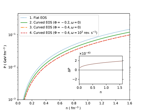
Figure 1: Plot of the pressure $P$ exerted by an ensemble of degenerate neutrons inside a slowly rotating ideal neutron star as a function of total neutron number density $n$ for different kinematical values of $\Phi$ and $\omega$. Here $\omega$ is specified in the unit of revolution per second. We note that the curves $3$ and $4$ with different values of $\omega$ are effectively indistinguishable. The difference between the curves $3$ and $4$ i.e. $\Delta P\equiv P_{4}-P_{3}$ is shown in the inset plot using same units as the main plot. It shows that effect of dragging of inertial frames on the pressure, described by $\omega$, is extremely small. In contrast, the effect of gravitational time-dilation on the pressure, described by $\Phi$, is considerably large.

However, the Einstein equation is not directly sensitive to the neutron number density $n$. Its dependence on the Einstein equation enters through the pressure $P$ and the energy density $\rho$. So it is more apt to look at the dependence of the pressure $P$ on the energy density $\rho$. The ratio $P/\rho$ is plotted as a function of the energy density $\rho$ in the FIG. 2. From the figure, we observe that the gravitational time dilation as well as the dragging of inertial frames both lead to an enhancement of the pressure $P$ for a given energy density $\rho$. In other words, the effect of curved spacetime of a slowly rotating star makes a degenerate equation of state stiffer compared to its counterpart which is computed in the Minkowski spacetime. The gravitational time dilation effect, arising due to the varying metric function $\Phi$, leads to a significant enhancement of the pressure $P$ compared to its flat spacetime counterpart. However, similar enhancement due to the dragging of inertial frames, parameterized by the metric function $\omega$, is extremely small. We may mention here that the curved EOS depends directly on the frame-dragging angular velocity $\omega$ rather than the angular velocity $\Omega$ of the stellar fluid. Nevertheless, a non-vanishing frame-dragging angular velocity $\omega$ follows from a non-vanishing angular velocity of the stellar fluid $\Omega$ through the solution of the Einstein equation (10) i.e. $\omega=\omega(r,\Omega)$. The radial variations of $\omega$ for different parameter values are shown in the FIG. 3.

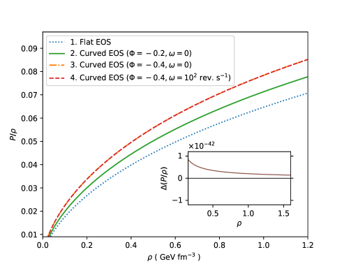
Figure 2: Plot of the ratio $P/\rho$ as a function of the energy density $\rho$ for different kinematical values of the metric functions $\Phi$ and $\omega$. The curves $3$ and $4$ with different values of $\omega$ are indistinguishable as earlier. The difference between these two curves i.e. $\Delta(P/\rho)\equiv(P/\rho)_{\omega}-(P/\rho)_{\omega=0}$ is shown in the inset plot using same unit for $\rho$ as the main plot. As earlier, we note that the effect of gravitational time-dilation on the equation of state is large whereas the effect of frame-dragging is extremely small.

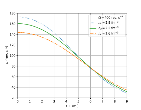
Figure 3: The radial variations of frame-dragging angular velocity $\omega$, for different values of the central neutron number density $n_{c}$, inside an ideal neutron star whose stellar fluid is revolving $400$ times per second.

V.1 Solution of the Einstein equation

In general, a rotating star has a shape of an oblate sphere. However, a slowly rotating star can be analyzed by decomposing it into a part that corresponds to a non-rotating ‘spherical’ star and a set of perturbative corrections to its mass and radius which are $\mathcal{O}(\omega^{2})$ Hartle (1967). In this article, we have computed the curved EOS which includes corrections up to $\mathcal{O}(\omega)$. Therefore, we restrict our analysis here for the ‘spherical’ part of the star. In other words, in our analysis we ignore terms which are $\mathcal{O}(\omega^{2})$ or higher.

We note that the curved EOS (41, 42) can be viewed as $P=P(n,\Phi,\omega)$ and $\rho=\rho(n,\Phi,\omega)$. However, due to the breaking of spin-degeneracy, it is convenient to treat them as $P=P(n_{+},\Phi,\omega)$ and $\rho=\rho(n_{+},\Phi,\omega)$. For simplicity, here we shall not stitch the curved EOS with a separate EOS for the crust matter near the star surface. So in numerical scheme for solving Einstein’s equation, below the threshold number density $n_{0}$, we shall restrict $n_{-}$ to remain zero until $n_{+}$ vanishes at the surface thereby defining the radius of the ‘spherical’ part of the star $R$, as $n_{+}(R)=0$. However, for a slowly rotating star the threshold number density $n_{0}$ is extremely small. For example, the ratio $(\omega/m)\sim 10^{-22}$ for an ideal neutron star which is revolving a hundred times per second. So for a slowly rotating star the threshold number density $n_{0}$ lies way below the numerical precision which is used to define $n_{+}(R)$ numerically.

It is convenient to decompose the second order differential equation (10) into two first order differential equations for $\omega$ and $\omega^{\prime}$. Consequently, the Einstein equation for a slowly rotating star can be expressed as a first order differential equation for the tuple $\{\mathcal{M},\Phi,n_{+},\omega,\omega^{\prime}\}$ where $n_{+}$ satisfies

$$\frac{dn_{+}}{dr}=-\frac{(\rho+P+({\partial P}/{\partial\Phi}))}{({\partial P}/{\partial n_{+}})}\frac{d\Phi}{dr}-\frac{({\partial P}/{\partial\omega})}{({\partial P}/{\partial n_{+}})}\frac{d\omega}{dr}~{}.$$ (43)

In the equation (43), the partial derivatives are evaluated as

$$\left(\frac{\partial P}{\partial\Phi}\right)_{n_{+},\omega}=P+\omega n_{-}~{},~{}\left(\frac{\partial P}{\partial\omega}\right)_{n_{+},\Phi}=-n_{-}~{},$$ (44)

together with

$$\left(\frac{\partial P}{\partial n_{+}}\right)_{\Phi,\omega}=\sum_{s}\frac{\partial P_{s}}{\partial n_{s}}\frac{\partial n_{s}}{\partial n_{+}}~{},~{}\frac{\partial P_{s}}{\partial n_{s}}=\frac{m(bn_{s})e^{\Phi}}{\mathcal{F}_{s}}~{},$$ (45)

where $\mathcal{F}_{s}=3(bn_{s})^{1/3}\sqrt{(bn_{s})^{2/3}+1}$ with $s\in\{+,-\}$, $(\partial n_{+}/\partial n_{+})=1$ and $(\partial n_{-}/\partial n_{+})=(\mathcal{F}_{-}/\mathcal{F}_{+})$.

In order to evolve the tuple numerically, a set of initial conditions $\{\mathcal{M}=0,\Phi_{c},n_{+c},\omega_{c},\omega^{\prime}=0\}$ is chosen at the center of the star. While the value for $n_{+c}$ can be chosen independently, the values for $\Phi_{c}$, $\omega_{c}$ are determined by imposing the relevant constraints. In particular, the chosen values for $\Phi_{c}$ and $\omega_{c}$ should be such that the tuple satisfies the desired boundary conditions as $e^{2\Phi(R)}=(1-2GM/R)$, and $\omega^{\prime}(R)=-3\omega(R)/R$ where $M=\mathcal{M}(R)$. The values for $\Phi_{c}$ and $\omega_{c}$ that satisfy these constraints, can be found within the desired numerical precision by using suitable bisection methods.

In the FIG. 4, the mass-radius relations for a slowly rotating ideal neutron star are plotted, by comparing the results due to the flat EOS and the curved EOS. From the figure, it is clear that the effect of gravitational time dilation leads to a significant enhancement of the maximum mass limit for a slowly rotating neutron star. The dragging of inertial frames also leads to an enhancement of the mass limit although by an extremely small amount in comparison. The later enhancement nevertheless depends on the angular velocity of the stellar fluid $\Omega$. In contrast, the mass-radius relations that follow from the flat EOS, has no dependence on the stellar fluid angular velocity $\Omega$.

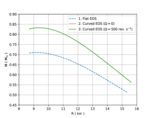
Figure 4: Comparison of the mass-radius relations for a slowly-rotating ideal neutron star whose degenerate core is made of an ensemble of non-interacting neutrons. Usage of the curved EOS leads to a much higher maximum mass limit compared to the usage of flat EOS. In particular, the effect of gravitational time dilation itself leads to an increase of maximum mass limit from $0.71$ M_⊙ to $0.83$ M_⊙. The enhancement of mass limit due to the dragging of inertial frames is however extremely small for any physically plausible values of stellar fluid angular velocity $\Omega$. We may note that the curves $2$ and $3$ with different values of $\Omega$ are nearly indistinguishable.

From the numerical solution of the tuple, the angular momentum of the star can be obtained as $J=\omega(R)R^{3}/2G$. In the FIG. 5, the angular momenta of a slowly rotating ideal neutron star are plotted, by comparing the usage of the curved EOS and the flat EOS. For a given set of values of the central number density $n_{+c}$ and the angular velocity of stellar fluid $\Omega$, the usage of curved EOS leads to a higher value for the angular momentum.

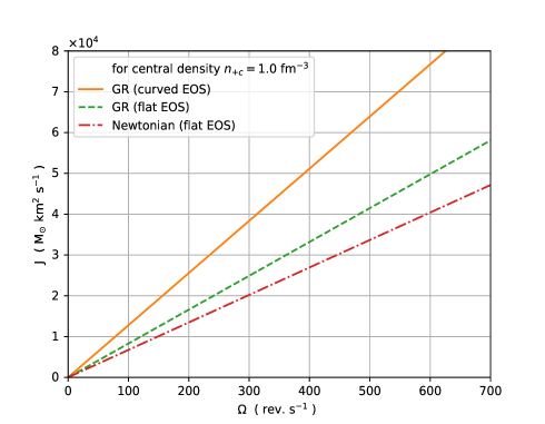
Figure 5: Comparison of the angular momenta of a slowly rotating ideal neutron star as a function of the angular velocity $\Omega$ of the stellar fluid. The Newtonian expression for the angular momenta is computed as $J=\Omega\int drd\theta d\varphi~{}\rho r^{4}\sin^{3}\theta$ where energy density $\rho=\rho(r)$ is taken to be the same as found by solving TOV equations with the flat EOS. It can be seen that the usage of the curved EOS, rather than the flat EOS, leads to higher values of angular momenta for a given value of central number density $n_{+c}$.

V.2 Effects of curved EOS on mass limits

The maximum mass limits of the compact stars such as the white dwarf stars or the neutron stars depend on the detailed nature of the EOS of constituent degenerate matter. The well-known Chandrasekhar mass limit of $1.4~{}M_{\odot}$ for the white dwarfs follows from the EOS which is computed by considering an ensemble of non-interacting degenerate electrons in a flat spacetime. By considering a similar approach, Oppenheimer had first shown that the maximum mass limit of neutron stars is around $0.71~{}M_{\odot}$ when one uses the EOS for an ensemble of non-interacting degenerate neutrons computed in a flat spacetime. Here we refer such a neutron star as an ideal neutron star. However, the mass limit derived by Oppenheimer fails to explain the astrophysical neutron stars whose masses are observed to be in the range from $1.1~{}M_{\odot}$ to more than $2~{}M_{\odot}$.

In the theoretical approach of Oppenheimer the neutrons within a neutron star are taken to be non-interacting but in reality such neutrons are believed to be strongly interacting. Unfortunately, the exact nature of nuclear matter interaction inside a neutron star is not known and it continues to be an open problem due to the incomplete understanding of Quantum Chromodynamics (QCD). So in order to produce higher mass limits of neutron stars, different models of nuclear matter interactions are considered in the literature.

The aim of the present article however is to study the effects of curved spacetime of a slowly rotating star on its degenerate matter EOS, the resultant masses and the angular momentum of these stars. In the neutron star literature, one usually computes the matter EOS by considering a globally flat spacetime rather than using the curved spacetime of the star. As shown here, the usage of the curved spacetime of a slowly rotating star contributes two different effects on the matter EOS, namely the effects due to the gravitational time-dilation and the frame-dragging.

In order to explicitly compute these effects on the matter EOS, for simplicity, here we have considered an ideal neutron star whose degenerate core consists of non-interacting neutrons. Subsequently, we have shown that the usage of curved spacetime leads to a significant enhancement of the maximum mass limit of the ideal neutron star from $0.71$ M_⊙ to $0.83$ M_⊙. However, such an increase alone cannot explain the existences of high mass neutron stars. Nevertheless, the authors have recently shown that the consideration of even simple $\sigma-\omega$ model of nuclear interactions in the curved spacetime of a non-rotating neutron star, leads to the mass limits that are more than $2M_{\odot}$ Hossain and Mandal (2021b). One can easily incorporate such a phenomenological model of nuclear interaction even in the curved spacetime of a slowly rotating neutron star as considered here, in order to obtain higher mass limits.

On the other hand, for the white dwarf stars the consideration of non-interacting degenerate electrons alone can lead to the maximum mass limit which can explain current astrophysical observations. In the FIG. 6, the mass-radius relations for a slowly-rotating white dwarf star are plotted. In particular, the usage of the curved spacetime of a slowly rotating white dwarf star leads to an enhancement of the Chandrasekhar mass limit form $1.416$ M_⊙ to $1.420$ M_⊙ .

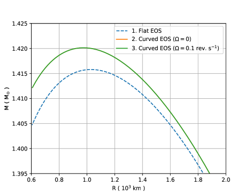
Figure 6: The mass-radius relations for a slowly-rotating white dwarf star whose degenerate core is made of an ensemble of non-interacting electrons. The energy density due to the nuclei is taken to be $\rho_{N}=(A/Z)m_{u}n_{e}e^{\Phi}$ where $n_{e}$, $m_{u}$, $A$ and $Z$ are the electron number density, atomic mass unit, atomic mass number and atomic number respectively Hossain and Mandal (2021a). For simplicity, here we have taken $A/Z=2$. Similar to the case of neutron star, usage of the curved EOS leads to a higher maximum mass limit compared to the usage of flat EOS. We note that the curves $2$ and $3$ with different values of $\Omega$ are nearly indistinguishable. In other words, the enhancement of the mass limit due to the dragging of inertial frames is extremely small in comparison to the time-dilation effect.

We note that for both neutron stars and white dwarfs the effects of curved spacetime manifest through the gravitational time-dilation effect and the frame-dragging effect. The effect on the mass limit due to the frame-dragging however is extremely small in comparison to the time-dilation effect. By using the expansion of the EOS (41, 42) as $\rho(n,\Phi,\omega)=\rho(n,\Phi,0)+\mathcal{O}((\omega/m)^{2})$, subject to the constraint (10), one can estimate the enhancement $\Delta M$ of the mass $M=\int_{0}^{R}4\pi r^{2}\rho$ as $\Delta M/M\sim(\Omega/m)^{2}$. We have discussed earlier that the ratio $(\Omega/m)\sim 10^{-22}$ for an ideal neutron star which is revolving a hundred times per second and its tiny effects on the EOS can be seen in the FIG. 1 and FIG. 2.

V.3 Speed of sound and causality

It can be seen from the FIG. 2 that the effects of gravitational time dilation and the dragging of inertial frames both lead the equation of state to become relatively stiffer compared to its flat spacetime counterpart. If the frame-dragging effect is turned off i.e if we set $\omega\to 0$ then the squared speed of sound $c_{s}^{2}\equiv(dP/d\rho)$ reduces to the one corresponding to a spherical spacetime which was shown to respect the causality Hossain and Mandal (2021a). For high neutron number densities i.e. $(bn_{\pm})\gg 1$, the pressure becomes $P\approx(e^{\Phi}m^{4}/24\pi^{2})[(bn_{+})^{4/3}+(bn_{-})^{4/3}]$ whereas the energy density becomes $\rho\approx(e^{\Phi}m^{4}/8\pi^{2})[(bn_{+})^{4/3}+(bn_{-})^{4/3}]$. This in turn implies that at higher densities, irrespective of the values $\Phi$ and $\omega$, the squared speed of sound can be expressed as

$$c_{s}^{2}=\frac{dP}{d\rho}\simeq\frac{1}{3}~{}.$$ (46)

At lower densities, as it can bee seen from the FIG. 2, the equation of state becomes relatively less stiffer. Therefore, the propagation speed of sound within the degenerate matter described by the curved EOS, respects causality for both higher and lower neutron number densities.

VI Discussions

In summary, we have presented a first-principle derivation of the equation of state for an ensemble of degenerate fermions by using the curved spacetime of a slowly rotating star. The derived equation of state is directly applicable for the studies of degenerate stars such as the neutron stars as well the white dwarf stars. We have shown that in contrast to the equation of states that are computed in a globally flat spacetime and routinely used in the study of neutron stars in the literature, the equation of state computed in the curved spacetime depends on two key effects of the general theory of relativity, namely the gravitational time dilation effect and the frame-dragging effect. Further, we have shown that both of these effects lead to a relatively stiffer equation of state which in turn enhances the maximum mass limit of the neutron stars. We have also shown that for a given central number density the usage of curved spacetime in computing matter EOS, rather than a globally flat spacetime, leads to a relatively higher angular momentum for these stars.

The effect due to the gravitational time dilation however has much stronger impact on stiffening of the equation of state as compared to the impact of the frame-dragging effect. Nevertheless, in general relativity, a non-vanishing frame-dragging effect is essential to obtain a non-vanishing angular momentum for a rotating star. Further, we have shown here that the frame-dragging effect leads to a novel mechanism for stiffening of equation of states by breaking the spin-degeneracy of fermions. We are aware that one can also have breaking of spin-degeneracy under the influence of an external magnetic field. Since most of the compact stars such as the neutron stars are known to contain large magnetic fields such a symmetry breaking of the spin-degeneracy is expected to be much larger. Thus the mechanism as seen here suggests one to explore the effect of external magnetic field on stiffening equation of state due to the breaking of spin-degeneracy and to study its consequences. In addition, we note that the breaking of spin-degeneracy due to the frame-dragging effect also leads to a novel mechanism for generation of seed magnetism in spinning astrophysical bodies Hossain and Mandal (2022). Finally, we have seen that the effect of curved spacetime on the equation of state is quite significant in the case of a neutron star. So the results as shown here suggest a re-look at the various studies related to the neutron star that are performed using equation of states computed in a globally flat spacetime.