Abstract

We review dark energy models which can present non-negligible fluctuations on scales smaller than Hubble radius. Both linear and nonlinear evolutions of dark energy fluctuations are discussed. The linear evolution has a well-established framework, based on linear perturbation theory in General Relativity, and is well studied and implemented in numerical codes. We highlight the main results from linear theory to explain how dark energy perturbations become important on the scales of interest for structure formation. Next, we review some attempts to understand the impact of clustering dark energy models in the nonlinear regime, usually based on generalizations of the Spherical Collapse Model. We critically discuss the proposed generalizations of the Spherical Collapse Model that can treat clustering dark energy models and their shortcomings. Proposed implementations of clustering dark energy models in halo mass functions are reviewed. We also discuss some recent numerical simulations capable of treating dark energy fluctuations. Finally, we make an overview of the observational predictions based on these models.

0 0 0 https://doi.org/ A short review on clustering dark energy Title Ronaldo C. Batista 0000-0002-7655-8719 Ronaldo C. Batista Batista, R. C. Correspondence: rbatista@ect.ufrn.br A short review on clustering dark energy

1 Introduction

Since the discovery of the accelerated expansion of the Universe Riess et al. (1998); Perlmutter et al. (1999), a great variety of explanations have been proposed. The most simple and well-studied proposal is that the accelerated expansion is caused by the Cosmological Constant, $\Lambda$, which is constant in space and time and naturally possesses no fluctuations. In this model, Dark Energy (DE) only modifies the background cosmological evolution, then the modifications in linear and nonlinear evolution of cosmological perturbations are straightforward to implement. Together with the Cold Dark Matter (CDM), which accounts for roughly $25\%$ of the Universe energy density, the $\Lambda$CDM model provides an outstanding description of cosmological data obtained so far, e.g., Aghanim et al. (2020); Abbott et al. (2021); Asgari et al. (2021)

Although $\Lambda$CDM is very successful in describing almost all cosmological observations, on theoretical grounds, it is challenged by the Cosmological Constant Problem Weinberg (1989); Carroll (2001) and the Cosmic Coincidence Problem Zlatev et al. (1999). More recently, direct measurements of the Hubble constant, $H_{0}$, have also been challenging the $\Lambda$CDM model, showing a disagreement of about $5\sigma$ with respect to the inferred value from Cosmic Microwave Background (CMB) data Verde et al. (2019); Di Valentino et al. (2021). A less significant tension, about $3\sigma$, in the $\Lambda$CDM model is related to the predicted normalization of the matter power spectrum, $\sigma_{8}$, the $S_{8}=\sigma_{8}\sqrt{\Omega_{m0}/0.3}$ parameter Perivolaropoulos and Skara (2021); Di Valentino et al. (2021). A recent analysis of possible solutions can be found in Schöneberg et al. (2021).

Given these difficulties with $\Lambda$, a profusion of alternative models to explain the cosmic acceleration were proposed. One of the first and most popular alternatives to $\Lambda$ is the quintessence class of models. In these models, a new scalar field minimally coupled to gravity and with no direct interactions to other types of matter plays the role of DE. This kind of model was studied even before the discovery of accelerated expansion by Peebles and Ratra (1988); Wetterich (1988). In quintessence models, DE is time-dependent and its Equation of State (EoS) parameter track the background, possibly alleviating the Coincidence Problem Caldwell et al. (1998); Zlatev et al. (1999); Steinhardt et al. (1999).

Since the quintessence field is dynamical, it necessarily has fluctuations. These fluctuations, however, are relevant only on scales of the order of Hubble radius Ma et al. (1999); Brax et al. (2000); DeDeo et al. (2003). On the small scales of interest for structure formation, quintessence perturbations are much smaller than matter (dark matter plus baryons) perturbations and thus are usually neglected. This tiny amount of DE perturbations on small scales is a consequence of the sound speed of the field perturbations, which has a constant value $c_{s}=1$. This value of the sound speed implies that the sound-horizon scale of quintessence, a scale below which the perturbations are strongly suppressed by pressure support, is of the order of Hubble radius, $c_{s}/H_{0}$.

One of the first proposed models beyond the quintessence that can possible present relevant perturbations on small scales is the tachyon scalar field Sen (2002); Padmanabhan (2002); Bagla et al. (2003). The main difference with respect to quintessence is that the tachyon field has a time-varying speed of sound, which can be smaller than unity, thus allowing the field to cluster more effectively on smaller scales.

It was also observed that even more general scalar field models could be constructed. The so-called k-essence models were initially proposed in the context of Inflation Armendariz-Picon et al. (1999); Garriga and Mukhanov (1999). In such models, one has the freedom to choose both the kinetic term and the potential of the scalar field, which translates into liberty to choose the EoS parameter and $c_{s}$. Therefore, in this class of models, DE can have an arbitrarily low speed of sound, thus its perturbations can be the same order of magnitude of matter perturbations. In this scenario, DE has the potential to impact structure formation beyond the background level.

More recently, the class of Horndesky theories, Horndeski (1974), was rediscovered and it was shown that both quintessence and k-essence models are sub-classes of Horndesky. At the linear perturbation level, these sub-classes are parameterized by the $\alpha_{K}$ parameter Bellini and Sawicki (2014). In the context of Horndesky theories, many models beyond k-essence exist, including non-minimally coupled scalar fields, which also modify gravitational interaction. The various types of models that can explain the accelerated expansion can also be described in the Effective Field Theory framework Gubitosi et al. (2013). Many of these proposals are discussed in Amendola et al. (2018).

In this review, we will focus on DE models described by minimally coupled to gravity scalar fields. We also restrict our attention to fields with no direct interaction with other matter fields. The k-essence class of models can be parametrized as perfect fluids defined by two time-dependent functions, $w\left(t\right)$ and $c_{s}\left(t\right)$ and this description will suffice to analyze how large DE fluctuations can be and estimate their observational impact.

The first step to understand DE fluctuations is to study them at the linear perturbative level, which is described by the well-established theory of linear cosmological perturbations, e.g., Kodama and Sasaki (1984); Mukhanov et al. (1992); Ma and Bertschinger (1995). In this context, the study of DE perturbations is straightforward, but limited to large scales that did not develop nonlinear matter fluctuations. Difficulties arise when trying to study DE fluctuations in the nonlinear regime. Historically, structure formation was studied using the Newtonian theory, which can not deal with relativistic fluids, such as DE. The obvious approach of using full-blown General Relativity to include DE fluctuations in structure formation studies is undoubtedly challenging. In fact, relativistic studies of structure formation with Clustering Dark Energy (CDE) were developed quite recently Dakin et al. (2019); Hassani et al. (2019, 2020).

The first attempt to study Clustering DE (CDE) models in the nonlinear regime used an integration between the Newtonian Spherical Collapse Model (SCM) with a “local” Klein-Gordon equation, modified to permit the clustering of quintessence Mota and van de Bruck (2004). This study was able to show important new effects due to DE fluctuations, which were later confirmed by more general and well-justified models. For instance, depending on the evolution of its EoS, DE fluctuations can become nonlinear, impact the nonlinear evolution of matter fluctuations and change the virialization state of matter halos. Hence, it became clear that CDE can impact structure formation. Later on, some authors constructed a more formal and general framework to include CDE in the SCM, Abramo et al. (2007); Creminelli et al. (2010); Basse et al. (2011).

The main focus of this review is to describe and discuss the applicability of the generalizations of the SCM capable of treating CDE models. We also pay special attention to the corresponding modifications on the Halo Mass Functions (HMF), which, up to now, have not been explored by numerical simulations. Moreover, we review the impact of CDE on cosmological observables and prospects for its detection.

The plan for this review is the following. Section 2 presents the essentials of relativistic perturbation theory that describe DE perturbations and their scale dependence. In Section 3, we review quintessence and k-essence models, highlighting the conditions under which relevant DE perturbations can be present. Section 4 discusses the SCM and its generalizations to study homogeneous and inhomogeneous DE models. Section 5 presents the Pseudo-Newtonian description of the SCM, which permits direct contact with linear relativistic perturbations on small scales and provides a clear and general framework to study CDE models in the nonlinear regime. We discuss the impact of DE fluctuations on the critical density threshold and HMF in Sections 6 and 7, respectively. The observational impact of CDE is reviewed in Section 8. We discuss the main results and perspectives in Section 9.

2 Linear perturbations

To understand the basic behaviour of DE perturbations, it is enough to consider scalar perturbations in the absence of anisotropic stresses. In this case, the perturbed line element in the Newtonian gauge is given by Ma and Bertschinger (1995)

$$ds^{2}=a^{2}\left(\eta\right)\left[-\left(1+2\Phi\right)d\eta^{2}+\left(1-2\Phi\right)d\vec{x}^{2}\right]\,,$$ (1)

where $\eta$ is the conformal time and $\Phi$ the gravitational field. The energy momentum of a perfect fluid with energy density $\rho$, pressure $p$ and four-velocity $u_{\mu}$ is given by

$$T_{\mu\nu}=\left(\rho+p\right)u_{\mu}u_{\nu}-pg_{\mu\nu}\,,$$ (2)

which include background (overbar quantities) plus perturbed quantities: $\rho=\bar{\rho}+\delta\rho$, $p=\bar{p}+\delta p$, $u_{\mu}=\bar{u}_{\mu}+v_{\mu}$.

We also restrict the analysis to the matter dominated era and the actual DE dominated phase. Then, at background level, we have the Friedman equations including matter (barions plus dark matter, indicated by the subscript $m$) and dark energy (indicated by the subscript $de$) given by

$$\mathcal{H}^{2}\equiv\left(\frac{a^{\prime}}{a}\right)^{2}=\frac{8\pi G}{3}a^{2}\left(\bar{\rho}_{m}+\bar{\rho}_{de}\right)\,,$$ (3)

$$\mathcal{H}^{\prime}=-\frac{4\pi G}{3}\left(\bar{\rho}_{m}+\bar{\rho}_{de}\left(1+w\right)\right)\,,$$ (4)

where $w=\bar{p}_{de}/\bar{\rho}_{de}$ is the EoS parameter for DE and the prime indicates derivative with respect to the conformal time, $\eta$. Density parameters of matter and DE are defined by

$$\Omega_{m}=\frac{\bar{\rho}_{m}(a)}{\rho_{c}(a)}\,\,\,\mbox{and}\,\,\,\Omega_{de}=\frac{\bar{\rho}_{de}(a)}{\rho_{c}(a)}\,,$$ (5)

where $\rho_{c}=\bar{\rho}_{m}+\bar{\rho}_{de}$ is the critial density.

In this review, we present examples using the CPL parametrization of the EoS Chevallier and Polarski (2001); Linder (2003)

$$w=w_{0}+w_{a}\left(1-a\right)\,,$$ (6)

where $w_{0}$ and $w_{a}$ are constants. Since $\Lambda$ gives a good description for the background evolution, we fix $w_{0}=-1$ and will vary $w_{a}$ to show the impact of DE fluctuations in a scenario that is very similar to $\Lambda$CDM at low redshift.

In Fourier space, the $\left(00\right)$ component of Einstein equations is given by

$$k^{2}\Phi+3\mathcal{H}\left(\Phi^{\prime}+\mathcal{H}\Phi\right)=4\pi Ga^{2}\left(\bar{\rho}_{m}\delta_{m}+\bar{\rho}_{de}\delta_{de}\right)\,,$$ (7)

where $\delta_{\ell}=\delta\rho_{\ell}/\bar{\rho}_{\ell}$ is the density contrast for a given component identified by the subscript $\ell$. The conservation equations for perturbations of each fluid component, $\nabla^{\nu}\delta T_{\nu}^{\mu}=0$, can be written as

$$\delta^{\prime}+3\mathcal{H}\left(\delta p/\delta\rho-w\right)\delta+\left(1+w\right)\left(\theta-3\Phi^{\prime}\right)=0$$ (8)

$$\theta^{\prime}+\mathcal{H}\left(1-3c_{a}^{2}\right)\theta=k^{2}\Phi+\frac{\delta p/\delta\rho k^{2}\delta}{1+w}\,,$$ (9)

where $\theta=ik^{j}v_{j}$ is the divergence of the fluid peculiar velocity and $c_{a}^{2}=\bar{p}^{\prime}/\bar{\rho}^{\prime}$ is the adiabatic sound speed of the fluid. The pressure perturbation is given by Bean and Dore (2004)

$$\delta p=c_{s}^{2}\delta\rho+3\mathcal{H}\left(1+w\right)\left(c_{s}^{2}-c_{a}^{2}\right)\bar{\rho}\frac{\theta}{k^{2}}\,,$$ (10)

where $c_{s}^{2}=\left(\delta p/\delta\rho\right)_{{\rm rest}}$ is the sound speed of the fluid in its rest frame.

An adiabatic or barotropic fluid is defined by $c_{s}=c_{a}$. The fluid is said to possess entropy perturbation if $c_{s}\neq c_{a}$. In general, DE models have entropy perturbations, but it is also possible to construct adiabatic models, e.g., Linder and Scherrer (2009); Unnikrishnan and Sriramkumar (2010)

Let us analyze the behaviour of perturbations in an adiabatic DE model, which has simpler equations – see Ballesteros and Lesgourgues (2010) for a more general treatment. In this case, the last term in (10) vanishes. Assuming $w$ and $c_{s}$ as constants, from (8)-(10) we can determine a second order equation for DE density contrast

$$\delta_{de}^{\prime\prime}+\mathcal{H}\left(1-3w\right)\delta_{de}^{\prime}+\left[3\mathcal{H}^{\prime}\left(c_{s}^{2}-w\right)+3\mathcal{H}^{2}\left(c_{s}^{2}-w\right)\left(1-3c_{s}^{2}\right)+c_{s}^{2}k^{2}\right]\delta_{de}\\ =-\left(1+w\right)\left[k^{2}\Phi-3\mathcal{H}\left(1-3c_{s}^{2}\right)\Phi^{\prime}-3\Phi^{\prime\prime}\right]\,.$$ (11)

Let us focus on small scales, $k^{2}\gg\mathcal{H}^{2},\mathcal{H}^{\prime}$ and $k^{2}\Phi\gg\mathcal{H}\Phi^{\prime},\Phi^{\prime\prime}$. During the matter dominated era, we have the well-known solution $\delta_{m}\propto a$ and $\Phi=\text{constant}$, and equation (11) simplifies to

$$\delta_{de}^{\prime\prime}+\mathcal{H}\left(1-3w\right)\delta_{de}^{\prime}+c_{s}^{2}k^{2}\delta_{de}=-\left(1+w\right)k^{2}\Phi\,.$$ (12)

For non-negligible $c_{s}^{2}$, equation (11) has a constant solution

$$\delta_{de}=-\frac{\left(1+w\right)}{c_{s}^{2}}\Phi\,.$$ (13)

Since, from (7), $\delta_{m}\sim k^{2}\Phi$, DE perturbations are usually negligible on small scales when compared to the matter perturbations.

For negligible $c_{s}$, equation (11) has the following solution Abramo et al. (2009); Sapone et al. (2009); Creminelli et al. (2009)

$$\delta_{de}=-\frac{\left(1+w\right)}{\left(1-3w\right)}\delta_{m}\,,$$ (14)

which is a good approximation even for Early DE models Batista and Pace (2013).

As can be seen, the magnitude of DE perturbations is determined by both $w$ and $c_{s}$. If $w\simeq-1$, as should be at low-$z$, DE perturbations are strongly suppressed regardless of $c_{s}$. For DE models in which $w$ deviates from $-1$ at higher redshift and with low or negligible $c_{s}$, DE perturbations can be as large as matter perturbations in the matter-dominated era, as indicated by (14). As we will see, in this case, DE fluctuations can become nonlinear and impact structure formation.

The solution (14) also indicates a correlation between matter and DE perturbations. Positive matter perturbations, which will be associated with the formation of halos in the nonlinear regime, will induce DE overdensities in the case of $1+w>0$ and underdensities if $1+w<0$. As we will see later, in the nonlinear regime, this correlation can induce a pathological behaviour for phantom DE models ($w<-1$), namely, $\delta_{de}<-1$.

The comoving scale bellow which DE perturbations are strongly suppressed by its pressure support is given by the sound horizon

$$r_{s}=\int_{a_{i}}^{1}\frac{c_{s}da}{a^{2}H}\,,$$ (15)

here $H=\dot{a}/a$ is the usual Hubble parameter and the dot indicates derivative with respect to time. In regions below this scale, the pressure support halts the growth of DE perturbations. As we will see, quintessence models have $c_{s}=1$, then $r_{s}\sim 1/H_{0}$ and their perturbations are very small on scales below the Hubble radius.

Let us estimate the value of $c_{s}$ that induce large DE perturbations on small scales. For instance, $c_{s}=10^{-3}$ gives a sound horizon $r_{s}\simeq 14\text{Mpc}$ (assuming best fit Planck18 cosmology Aghanim et al. (2020)). This value is associated with a mass scale $M=4\pi/3\bar{\rho}_{m0}\left(r_{s}/2\right)^{3}\simeq 2\times 10^{14}M_{\odot}$, where $\rho_{m0}$ is the matter density now. The value $c_{s}=10^{-3}$ was indeed reported to impact the formation of halos of such mass by Basse et al. (2011). As we will discuss later, in this work the authors considered that DE fluctuations do not break linear approximation. In the limit of $c_{s}\rightarrow 0$, however, DE fluctuations can become nonlinear, depending on the value of $w$. Nevertheless, we can consider that impact of DE fluctuations to become important for nonlinear structure formation for $c_{s}<10^{-3}$.

3 Dark Energy Models

Now that we have understood under which circumstances DE perturbations can be significant on small scales, let us discuss some DE models that can present such large perturbations. The variety of DE models is enormous, with several reviews, books and extensive analysis about them, e.g., Copeland et al. (2006); Amendola and Tsujikawa (2010); Yoo and Watanabe (2012); Tsujikawa (2013); Ade et al. (2016). We will focus on the k-essence class of models, which provide enough generality for $w$ and $c_{s}$ to permit large DE perturbations.

Models of k-essence were initially introduced in the context of inflation Armendariz-Picon et al. (1999); Garriga and Mukhanov (1999) and shortly after applied to describe DE Armendariz-Picon et al. (2001); Erickson et al. (2002). A cosmological model with k-essence is described by the following action

$$S=\int d^{4}x\sqrt{-g}\left[-\frac{\mathcal{R}}{2\kappa^{2}}+\mathcal{L}\left(X,\varphi\right)\right]+S_{m}\,,$$ (16)

where $\kappa^{2}=8\pi G$, $\mathcal{R}$ is the Ricci scalar, $X=-\frac{1}{2}g^{\mu\nu}\partial_{\mu}\varphi\partial_{\mu}\varphi$, $\mathcal{S}_{m}$ the action for matter fields (photons, neutrinos, baryons, dark matter) and $\mathcal{L}\left(X,\varphi\right)$ the Lagrangian for the k-essence field, $\varphi$. The k-essence energy-momentum tensor is given by

$$T_{\mu\nu}=\mathcal{L}_{,X}\nabla_{\mu}\varphi\nabla_{\nu}\varphi-\mathcal{L}g_{\mu\nu}\,,$$ (17)

where subscript $,X$ represents the derivative with respect to $X$. Comparing it to the perfect fluid energy momentum tensor (2), we find that

$$\rho=2X\mathcal{L}_{,X}-\mathcal{L}\,,\,\,\,p=\mathcal{L}\,\text{ and }u_{\mu}=\frac{\nabla_{\mu}\varphi}{\sqrt{2X}}\,.$$ (18)

The sound speed of k-essence perturbations is given by Garriga and Mukhanov (1999)

$$c_{s}^{2}=\frac{p_{,X}}{\rho_{,X}}\,.$$ (19)

In this framework it is clear that one has the freedom to choose the functions $w$ and $c_{s}$. Next, let us have a look at some specific popular realizations of DE models.

3.1 Quintessence

In the k-essence language, quintessence is defined by $\mathcal{L}=X-V\left(\varphi\right)$, then its EoS parameter, defined by $p/\rho$ given by (18), and sound speed, given by (19), read

$$w=\frac{X-V}{X+V}\,\text{ and }c_{s}^{2}=1\,.$$ (20)

If the kinetic energy of the field dominates over its potential energy, we have $w\simeq 1$. In the opposite case, $w\simeq-1$. Its sound speed, however, is always the same. Hence, although $w$ can be far from $-1$, the sound speed of quintessence does not allow for large perturbations on small scales.

This fact can also be understood via the Klein-Gordon equation for quintessence perturbations, which can be written as chan Hwang and Noh (2001)

$$\delta\ddot{\varphi}+3H\delta\dot{\varphi}+\left(c_{s}^{2}k^{2}+\frac{d^{2}V}{d\varphi^{2}}\right)\delta\varphi=\dot{\varphi}\delta_{m}\,,$$ (21)

where we explicitly introduced the the parameter $c_{s}$. Quintessence models must have $V\sim H_{0}^{2}$ in order to accelerate the Universe expansion recently, where $H_{0}=H(t_{0})$ is the Hubble constant. Thus, for scales well bellow the Hubble radius, $c_{s}^{2}k^{2}\gg\frac{d^{2}V}{d\varphi^{2}}$, and the field perturbations are strongly suppressed on these scales.

Since quintessence was initially the most popular alternative model to $\Lambda$, initially, many cosmologists considered DE perturbations were effectively negligible on small scales. This picture started to change with the appearance of new DE models which can have $c_{s}<1$.

3.2 Tachyon

A well-known model for DE that makes use of non-canonical scalar field is the tachyon field. It was introduced in the context of string theory Sen (2002, 2002), but can also be understood as a generalization of the relativistic particle lagrangian, Padmanabhan and Choudhury (2002). The tachyon model is defined by the following lagrangian

$$\mathcal{L}=-V\left(\varphi\right)\sqrt{1-2X}\,,$$ (22)

Comological studies of this model include Padmanabhan (2002); Padmanabhan and Choudhury (2002); Bagla et al. (2003); Abramo and Finelli (2003). The EoS parameter and its sound speed are given by

$$w=2X-1\,\text{ and }c_{s}^{2}=-w$$ (23)

The accelerated expansion occurs when $X\ll 1$, thus $w\simeq-1$ and $c_{s}^{2}\simeq 1$. In this case, the behaviour is very similar to quintessence. However, earlier in the cosmological history, the kinetic term can be larger, which yields a smaller $c_{s}$. In this case, both $w$ and $c_{s}$ provide the conditions for large DE perturbations.

Considering a power-law potential, $V\left(\varphi\right)\propto\varphi^{-\alpha}$, the actual impact of tachyon perturbations on CMB is small because the accelerated expansion requires $\alpha\simeq 0$, which, in turn, suppresses the field perturbations Abramo et al. (2004). Nevertheless, this model clearly shows that DE perturbations are not necessarily small on scales below the Hubble radius.

For a constant potential, the tachyon model is equivalent to the Chaplygin gas Kamenshchik et al. (2001), with equation of state

$$p=-\frac{A}{\rho}\,,$$ (24)

where $A$ is a constant. This model and its generalized version was studied by many authors, e.g., Bento et al. (2002); Sandvik et al. (2004); Makler et al. (2003); Bento et al. (2003); Amendola et al. (2003); Reis et al. (2004). Both the tachyon and Chaplygin models gave rise to a scenario in which DE and dark matter can be considered manifestations of a single component, which became known as quartessence or unified dark energy Sahni and Wang (2000); Bilic et al. (2002), for a review of these ideas, see Bertacca et al. (2010).

3.3 Clustering DE

It is possible to construct DE models with negligible sound speed. In the context of k-essence, a model with a constant arbitrary $c_{s}$ is given by Kunz et al. (2015)

$$\mathcal{L}=M^{4}\left(\frac{X}{M^{4}}\right)^{\frac{1+c_{s}^{2}}{2c_{s}^{2}}}+V\left(\varphi\right)\,,$$ (25)

where $M$ is a constant mass scale. In the context of quartessence, Scherrer (2004) proposed a model with very low $c_{s}$. A possible issue when building such models is that distinct lagrangians can have the same $w$ and $c_{s}$, Unnikrishnan (2008).

In effective field theory, models with $c_{s}^{2}\sim-10^{-30}$ were described by Creminelli et al. (2009). Although negative $c_{s}^{2}$ yields gradient instabilities, this value is so small that no relevant effect on cosmological scales is expected. This work also concludes that no pathological behaviour is present for phantom models, $w<-1$. However, as we will show later on, in the nonlinear regime, it is possible that phantom DE with negligible sound speed can present $\delta_{de}<-1$, i.e., a pathological situation with negative energy density, $\rho_{de}=\bar{\rho}_{de}(1+\delta_{de}$).

Models with identically zero sound speed using two scalar fields were proposed by Lim et al. (2010). In Horndeski theories, there are even more possible realizations of DE with low sound speed, which can be chosen as a function of four physical parameters Bellini and Sawicki (2014).

Given the variety of possible CDE models, the phenomenological implementation of parametrizations of $w$ and $c_{s}$ is valuable to explore the possible impact of DE perturbations on structure formation. As already mentioned, we will show examples using $w=w_{0}+w_{a}\left(1-a\right)$ and constant $c_{s}$.

4 The spherical collapse model

Once we know the basic behaviour of DE linear perturbations, we may ask how they impact the structure formation on small scales. The SCM is an analytical approach first proposed to study the nonlinear evolution of matter perturbations in the Universe. It can be used in connection to analytic and semi-analytic halo mass functions to determine the abundance of matter halos, which we will describe in section 7. In this section, we will review the classic formulation of the SCM and the main quantities of cosmological interest. We also discuss some generalizations capable of treating homogeneous DE and the first proposed model that considers the nonlinear evolution of DE fluctuations. Later on, we will present a more general framework for the SCM and a detailed discussion about threshold density, which is an important quantity that determines the abundance of halos.

4.1 Einstein-de-Sitter Universe

The SCM was first proposed by Gunn and Gott (1972). The important conclusions for our porpouses are described in Padmanabhan (1993) and Sahni and Coles (1995). This model describes the dynamics of spherical shell of radius $R$ that encloses a mass $M_{m}$. The dynamical equation for the shell radius is

$$\ddot{R}=-\frac{GM_{m}}{R^{2}}\,,$$ (26)

where the dot indicate derivative with respect to time. The mass is given by

$$M_{m}=\frac{4\pi}{3}R^{3}\bar{\rho}_{m}\left(1+\delta_{m}\right)\,,$$ (27)

where $\delta_{m}$ is assumed to be the averaged density contrast inside the sphere of radius $R$, which can also be understood as a top-hat profile for the matter fluctuation. The total mass is supposed to be conserved, $dM_{m}/dt=0$, which yields the following equation for the matter contrast

$$\dot{\delta}_{m}+3\left(\frac{\dot{R}}{R}-\frac{\dot{a}}{a}\right)\left(1+\delta_{m}\right)=0\,,$$ (28)

which has the solution

$$\delta_{m}+1=\left(\delta_{mi}+1\right)\left(\frac{a}{a_{i}}\frac{R_{i}}{R}\right)^{3}\,,$$ (29)

where the subscripts $i$ indicate the initial values.

The first integral of (26) is given by

$$\frac{1}{2}\dot{R}^{2}-\frac{GM_{m}}{R}=E\,,$$ (30)

where $E$ is a constant of integration identified as the total energy of the shell – the kinetic energy ($K=\dot{R}^{2}/2$) plus the potential energy per unit of mass ($U=-GM_{m}/R$). Note that, in the derivation of (30), the fact that $M_{m}$ is constant was used. As we will see later on, in the presence of DE, the effective mass inside the shell is not conserved anymore.

Assuming that the shell initially expands with the background, $R\propto a$, we have $\dot{R}_{i}=H_{i}R_{i}$. Using (27), the total energy can be expressed as

$$E=\frac{\left(H_{i}R_{i}\right)^{2}}{2}\left[\frac{1}{\Omega_{mi}}-\left(1+\delta_{mi}\right)\right]\,,$$ (31)

where $\Omega_{mi}=\Omega_{m}\left(a_{i}\right)$. For $1+\delta_{mi}>1/\Omega_{mi}$, the total energy of the shell is negative. Thus it is expected that the initially expanding dust cloud will grow to a maximum radius, contract and eventually form a bounded structure. In EdS Universe, $\Omega_{m}=1$, and any region with positive $\delta_{mi}$ will eventually collapse. As we will see next, this is indeed the behaviour given by solving for the time evolution of $R$, which will describe the formation of a matter halo. On the other hand, if $1+\delta_{mi}<1/\Omega_{mi}$, the total energy of the shell is positive and the cloud will expand forever, forming a void with $-1<\delta_{m}<0$.

The maximum shell radius is given by $\dot{R}=0$ and is called the turn-around radius, given by

$$R_{ta}=R_{i}\frac{1+\delta_{mi}}{1+\delta_{mi}-1/\Omega_{mi}}\,.$$ (32)

This is indeed a maximum radius because equation (26) indicates that $\ddot{R}<0$. This fact also implies that no solution of a minimal radius exists in the usual SCM, and consequently, the model can not describe an equilibrium configuration. This shortcoming is usually circumvented by assuming that the system achieves virial equilibrium at some point of its evolution and that this state represents the final bounded structure. There were efforts in implementing virialization in the dynamics of the SCM, see Engineer et al. (2000); Shaw and Mota (2008).

Equation (26) can be solved analytically with the following parametrization

$$R=A\left(1-\cos x\right)\text{ and }t=B\left(\theta-\sin x\right)\,,$$ (33)

where $A=R_{ta}/2$, $B=t_{ta}/\pi$. Substituting these expressions in (26) one gets the relation $A^{3}=GM_{m}B^{2}.$

As can be seen from (33), the shell radius is maximum at $\theta=\pi$ (turn-around) and then begins to shrink. Formally, as $x\rightarrow 2\pi$, $R\rightarrow 0$ and, from (29), $\delta_{m}\rightarrow\infty$. This is identified as the moment of collapse. In reality, these values are not achieved because, for a given shell approaching collapse, other inner shells containing collisionless matter have already crossed each other. Thus, the total mass within a specific radius is not conserved anymore, signalling the break down of the model. Nevertheless, the collapse time is used to define quantities used to estimate the abundance of halos.

Using conservation of mass, given by equation (27), and the background density evolution in EdS $\bar{\rho}_{m}=\left(6\pi Gt^{2}\right)^{-1}$, the nonlinear evolution of matter fluctuations is given by

$$\frac{\rho_{m}}{\bar{\rho}_{m}}=1+\delta_{m}^{NL}=\frac{9}{2}\frac{\left(x-\sin x\right)^{2}}{\left(1-\cos x\right)^{3}}\,,$$ (34)

where the superscript $NL$ indicates the nonlinear value of the density constrast. Expanding for small $x$, we get the linear evolution

$$\delta_{m}^{L}=\frac{3}{5}\left(\frac{3}{4}\right)^{2/3}\left(x-\sin x\right)^{2/3}\,,$$ (35)

where the superscript $L$ indicates the linear value of the density contrast. At turn-around, we have

$$\delta_{m}^{NL}\left(x=\pi\right)=\frac{9\pi^{2}}{16}-1\simeq 4.552$$ (36)

and

$$\delta_{m}^{L}\left(x=\pi\right)=\frac{3}{5}\left(\frac{3\pi}{4}\right)^{2/3}\simeq 1.062\,.$$ (37)

As can be seen, at this time, the linear evolution gives a density contrast of order one, indicating the transition from linear to nonlinear regime.

The collapse threshold (or critical density contrast) is the extrapolated linear overdensity value above which a bound structure is considered formed, a halo. Usually, it is defined at the collapse time

$$\delta_{c}\equiv\delta_{m}^{L}\left(x=2\pi\right)=\frac{3}{5}\left(\frac{3\pi}{2}\right)^{2/3}\simeq 1.686\,.$$ (38)

As we will see later, the value $\delta_{c}$ is of great importance in structure formation studies that make use of analytic or semi-analytic mass functions. This quantity is modified in the presence of homogeneous and inhomogeneous DE.

It is also important to describe the state of equilibrium of the halo, which is assumed to obey the virial theorem for non-relativistic particles. Virialization occurs when $U\left(R_{{\rm v}}\right)=-2K\left(R_{{\rm v}}\right)$, were $R_{{\rm v}}$ is the virialization radius. At turn-around, $E=U\left(R_{ta}\right)=U\left(R_{{\rm v}}\right)+K\left(R_{{\rm v}}\right)$, then we get the relation

$$R_{{\rm v}}=\frac{R_{m}}{2}\,.$$ (39)

From this, we can compute the virialization time ($x=3\pi/2$)

$$t_{{\rm v}}=\left(\frac{3}{2}+\frac{1}{\pi}\right)t_{ta}\simeq 1.818t_{ta}\,.$$ (40)

The collapse time ($x=2\pi$) is

$$t_{coll}=2t_{m}\,.$$ (41)

With these quantities, two definitions of virialization overdensity are usually found in the literature. One possibility is define the virialization overdensity with respect to the matter background density

$$\Delta_{{\rm cm}}\equiv\frac{\rho_{m}\left(t_{v}\right)}{\bar{\rho}_{m}\left(t_{c}\right)}=18\pi^{2}\simeq 177.7\,.$$ (42)

Another common choice uses the critical density as reference

$$\Delta_{{\rm cc}}\equiv\frac{\rho_{m}\left(t_{v}\right)}{\bar{\rho}_{c}\left(t_{c}\right)}\,.$$ (43)

Of course, $\Delta_{{\rm cm}}$ and $\Delta_{{\rm cc}}$ give essentially the same results in a matter dominated Universe, but they differ when DE becomes important, see figure 1.

The overdensity $\Delta\thickapprox 178$ became a reference value used in N-body simulations in order to identify halos, but many other definitions can be used, see Despali et al. (2016) for an analysis of several such choices. Interestingly, this paper has shown that the use of the quantity $\Delta_{{\rm cc}}$ yields more universal mass functions, in the sense of its dependence on redshift and cosmological parameters. We will return to this discussion when dealing with the impact of CDE on halo mass functions.

Yet another possibility is to compute both the total and background densities at the virialization time, as suggested by Lee and Ng (2010). In this case the virialization overdensity is given by

$$\Delta_{{\rm v}}\equiv\frac{\rho_{m}\left(t_{v}\right)}{\bar{\rho}_{m}\left(t_{v}\right)}=\frac{9}{2}\left(\frac{3\pi}{2}+1\right)^{2}\simeq 146.8\,.$$ (44)

The value of $\Delta_{{\rm v}}$ is slightly smaller than $\Delta_{{\rm cc}}$. Later on, will show that in the presence of DE these two quantities decay with redshift, whereas $\Delta_{{\rm cm}}$ grows (see figure 1). Analogously, we can define the threshold density at virialization

$$\delta_{{\rm v}}\equiv\delta_{m}^{L}\left(x=\frac{3\pi}{2}\right)=\frac{3}{5}\left(\frac{3}{4}\right)^{2/3}\left(\frac{3\pi}{2}+1\right)^{2/3}\simeq 1.583\,.$$ (45)

4.2 Spherical collapse model with homogeneous dark energy

In the presence of homogeneous DE, the SCM has to be modified to include the effects of this new component on the dynamics of the shell radius. Now we have

$$\ddot{R}=-\frac{G}{R^{2}}\left(M_{m}+M_{de}\right)\,,$$ (46)

where

$$M_{de}=\frac{4\pi}{3}R^{3}\bar{\rho}_{de}\left(1+3w\right)$$ (47)

is the effective mass associated with homogeneous DE. This definition can be understood via the Poisson equation in the presence of a relativistic fluid

$$\nabla^{2}\Phi=4\pi G\left(\rho+3p\right)\,.$$ (48)

The first study of the equation (46) was done by Lahav et al. (1991) considering $\Lambda$ as a DE component. It was found that the ratio of virial to turn-around radius is smaller in the presence of $\Lambda$, given by the following expression

$$\frac{R_{{\rm v}}}{R_{{\rm ta}}}\simeq\frac{1-\eta/2}{2-\eta/2}\,,$$ (49)

where $\eta=\Lambda/4\pi G\bar{\rho}_{m}\left(t_{ta}\right)$. Thus, in the presence of $\Lambda$, the halo has to contract more with respect to EdS to achieve the virial equilibrium. This indicates that halos formed in the late Universe have a distinct structure than those formed at high-$z$, when DE was very subdominant.

Other authors have studied the SCM in the presence of $\Lambda$, e.g., Lacey and Cole (1993); Kitayama and Suto (1996). Although analytical solutions for $\delta_{c}$ and $\Delta_{cc}$ were found, the following fits presented by Kitayama and Suto (1996) became popular:

$$\delta_{c}\simeq\frac{3\left(12\pi\right)^{2/3}}{20}\left(1+0.0123\log_{10}\Omega_{m}\left(z\right)\right)$$ (50)

and

$$\Delta_{cm}\simeq 18\pi^{2}\left(1+0.4093w_{f}^{0.9052}\left(z\right)\right)\,,$$ (51)

where $w_{f}\left(z\right)=1/\Omega_{m}\left(z\right)-1$. Expression (50) shows that the the influence of $\Lambda$ on the critical threshold is very small, giving $\delta_{c}\left(z=0\right)\simeq 1.676$ for $\Omega_{m0}=0.3$ (only $0.64\%$ different than the EdS value). However, the change in virialization overdensity is much larger. We have $\Delta_{cm}\left(z=0\right)\simeq 334.2$ for $\Omega_{m0}=0.3$, about two times EdS value.

Studies of DE with constant $w$ were done by Wang and Steinhardt (1998); Weinberg and Kamionkowski (2003). The fitting functions proposed in the latter, shows variations of $\delta_{c}\left(z\right)$ bellow $0.56\%$ for $-1<w<-0.8$ with respect to the $\Lambda$CDM fit. For $\Delta_{cm}$ the differences are lower than $17\%$. The differences can be slightly larger in some quintessence models Mainini et al. (2003)

In figure 1, we show a plot of these three different definitions of virial overdensity. As discussed, the variations in $\delta_{c}$ due to homogeneous DE are very small and will be shown together with the case of CDE in figure 2.

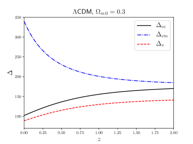
Figure 1: Redshift evolution of three virial overdensities definitions, equations (42), (43) and (44) for the $\Lambda$CDM model with $\Omega_{m0}=0.3$. In this plot, $\Delta_{{\rm v}}$ is determined using the method summarized by equation (78), while $\Delta_{cm}$ and $\Delta_{cc}$ by the proper numerical method discussed in section (6.1)

4.3 Spherical collapse model with inhomogeneous dark energy

The first study of SCM in the presence of CDE was done by Mota and van de Bruck (2004). DE was modeled as quintessence field, which equation of motion in background is given by

$$\ddot{\varphi}+3H\dot{\varphi}+\frac{dV}{d\varphi}=0\,.$$ (52)

Remind that, in the context of quintessence models, the fluctuations of such field must be tiny on small scales because $c_{s}=1$. The authors have considered, however, that the field can cluster on small scales, assuming that, inside the collapsing region, the it obeys the following equation

$$\ddot{\varphi}_{c}+3\frac{\dot{R}}{R}\dot{\varphi}_{c}+\frac{dV}{d\varphi_{c}}=\frac{\Gamma}{\dot{\varphi}_{c}}\,,$$ (53)

where

$$\Gamma=3\alpha\dot{\varphi}_{c}^{2}\left(\frac{\dot{R}}{R}-H\right)$$ (54)

is a quantity that describes the flux of DE in the collapsing region. If $\alpha=1$ DE evolves in the same way inside and outside the collapsing region, then DE is homogeneous, and $\varphi_{c}=\varphi$. On the other hand, if $\alpha=0$ the field can evolve differently than in the background, allowing for DE fluctuations. The impact on $\delta_{c}$ was computed in Nunes and Mota (2006), where differences of a few per cent with respect to $\Lambda$CDM and redshift dependent features associated with the evolution of $w$ were found.

Although this model was a breakthrough regarding the possibility of nonlinear fluctuations of DE, the implementation of equation (53) is ad doc and formally inconsistent with the Klein-Gordon equation, (21). Equation (53) can be interpreted as (21) with $c_{s}=0$, where the the gravitational coupling is encoded in the dynamics of $R$. Later it was shown that the canonical scalar field indeed has negligible perturbations on small scales Mota et al. (2007); Wang and Fan (2009). However, its perturbations can be more important on voids, which are much larger than halos.

Despite this inconsistency, this model presented some of the important impacts of DE fluctuations on the nonlinear regime, which were later confirmed by other studies. In particular, the following findings can be highlighted:

1. The amount DE fluctuations strongly depends on the evolution of $w$.

2. DE fluctuations impact the nonlinear evolution of $\delta_{m}$ and virialization of halos.

3. The local EoS of DE can be distinct from $w$ due to DE fluctuations.

4.4 Other generalizations of the spherical collapse model

Many other generalizations of the SCM were developed in the literature, including modifications due to coupled DE Manera and Mota (2006); Wintergerst and Pettorino (2010), modified gravity Martino et al. (2009); Schaefer and Koyama (2008); Schmidt et al. (2010); Brax et al. (2010); Borisov et al. (2012); Barreira et al. (2013); Kopp et al. (2013); Lopes et al. (2018, 2019); Frusciante and Pace (2020), varying vacuum models Basilakos et al. (2010), shear and rotation Del Popolo et al. (2013); Pace et al. (2014); Mehrabi et al. (2017), bulk viscosity Velten et al. (2014). In the next section we will present a framework that can describe the nonlinear evolution in the CDE model.

5 Spherical collapse model in the Pseudo-Newtonian Cosmology

General Relativity is the standard theory to study gravitational phenomena of fluids with relativistic pressure, $p\sim c^{2}\rho$. In the context of structure formation, the gravitational fields are small, and the weak field limit can be used. Therefore, one can consider using the Newtonian theory, but taking into account the effects of relativistic pressure. This approach was indeed used in McCrea (1951); Harrison (1965) to study the background evolution of the Universe. It was shown that Newtonian equations with the correction for relativistic pressure reproduce the Friedman equations.

However, the application of these modified Newtonian equations for the study of cosmological perturbations is more controversial. Sachs and Wolfe (1967) showed that perturbations in fluids with $p\neq 0$ do not agree with the relativistic treatment. For about three decades, the use of Newtonian equation for cosmology was halted until the origin of the discrepancy reported in 1967 by Sachs and Wolfe was found and treated in Lima et al. (1997).

According to Lima et al. (1997), the system of equations (the subscript $\ell$ identifies the different fluids under consideration), which we call Pseudo-Newtonian Cosmology (PNC),

$$\frac{\partial\rho_{\ell}}{\partial t}+\vec{\nabla}\cdot\left(\rho_{\ell}\vec{u}_{\ell}\right)+\frac{p_{\ell}}{c^{2}}\vec{\nabla}\cdot\left(\vec{u}_{\ell}\right)=0$$ (55)

$$\frac{\partial\vec{u}_{\ell}}{\partial t}+\left(\vec{u}_{\ell}\cdot\vec{\nabla}\right)\vec{u}_{\ell}=-\vec{\nabla}\Phi-\frac{\vec{\nabla}p_{\ell}}{\rho_{\ell}+\frac{p_{\ell}}{c^{2}}}$$ (56)

$$\nabla^{2}\Phi=4\pi G\sum_{\ell}\left(\rho_{\ell}+\frac{3p_{\ell}}{c^{2}}\right)$$ (57)

provides the correct growing modes for linear perturbations of fluids with relativistic pressure. The PNC was extensively studied and applied in the context of cosmological perturbations Reis (2003); Reis et al. (2004); chan Hwang and Noh (2006); Fabris et al. (2008); Abramo et al. (2009); Velten et al. (2013); Hwang et al. (2016). In particular, it was shown that PNC growing modes for DE perturbations agrees with the relativistic analysis Abramo et al. (2009).

The PNC can also be used to generalize the SCM Abramo et al. (2007, 2009). The perturbed equations in comoving coordinates with background are given by

$$\dot{\delta}_{\ell}+3H\left(c_{s\,\ell}^{2}-w_{\ell}\right)\delta_{\ell}+\left[1+w_{\ell}+\left(1+c_{s\,\ell}^{2}\right)\delta_{\ell}\right]\frac{\vec{\nabla}\cdot\vec{v}_{\ell}}{a}+\frac{\vec{v}_{\ell}\cdot\vec{\nabla}\delta_{\ell}}{a}=0\,,$$ (58)

$$\dot{\vec{v}}_{\ell}+H\vec{v}_{\ell}+\frac{\vec{v}_{\ell}\cdot\vec{\nabla}}{a}\vec{v}_{\ell}=-\frac{\vec{\nabla}\Phi}{a}-\frac{c_{s\,\ell}^{2}\vec{\nabla}\delta_{\ell}}{a\left[1+w_{\ell}+\left(1+c_{s\,\ell}^{2}\right)\delta_{\ell}\right]}\,,$$ (59)

$$\frac{\nabla^{2}\Phi}{a^{2}}=4\pi G\sum_{\ell}\bar{\rho}_{\ell}\delta_{\ell}\left(1+3c_{s\,\ell}^{2}\right)\,,$$ (60)

where $\vec{v}$ is the peculiar velocity of the fluid. Clearly, these equations are more general then those of the usual SCM. Let us consider the simplifying assumptions that will yield the correspondence between them.

Remind that the SCM assumes a top-hat profile, thus we need $\vec{\nabla}\delta=0$ inside the shell. The other quantities must be consistent with this assumption. Equation (58) must depend only on time, thus $\vec{\nabla}\cdot\vec{v}=\theta\left(t\right)$. Taking the divergence of (59) we get

$$\dot{\theta}_{\ell}+H\theta_{\ell}+\frac{\theta_{\ell}^{2}}{3a}=-4\pi Ga\sum_{\ell}\bar{\rho}_{\ell}\delta_{\ell}\left(1+3c_{s\,\ell}^{2}\right)$$ (61)

Now let us turn our attention to the parameter $c_{s}$. At first glance, assuming that $\vec{\nabla}\delta=0$ and $\vec{\nabla}\cdot\vec{v}=\theta\left(t\right)$ seems compatible to any choice $c_{s}=c_{s}\left(t\right)$. However, considering two distinct fluids, say pressureless matter ($w_{m}=c_{s\,m}=0$) and DE ($w_{de}=w_{de}\left(t\right)$ and $c_{s\,de}=c_{s\,de}\left(t\right)$), implies that each fluid has its own dynamical equation, (61). This indicates that there is no unique spherical shell radius, because the two fluids can flow with distinct velocities.

Another problem about using a generic function $c_{s}\left(t\right)$ arises when extending the analysis to regions outside the shell. For a top-hat profile, $\delta$ is discontinuous at the edge of the shell, then $\vec{\nabla}\delta$ is ill-defined at this point. A more realistic realization is to assume a smooth decay of $\delta$ around the edge. In this case, its gradient is well-defined and there exists a non-null pressure gradient, $c_{s}^{2}\vec{\nabla}\delta$, around the shell radius. This, again, would make the two fluids flow with distinct velocities and, more drastically, disrupt the original homogeneous top-hat-like profile.

Therefore, regarding the value of $c_{s}$, the equivalence of equations (58)-(60) with the usual SCM is achieved only for $c_{s}=0$. In this case, all fluids share the same dynamical equation and the evolution of the system is described by

$$\dot{\delta}_{\ell}-3Hw_{\ell}\delta_{\ell}+\left(1+w_{\ell}+\delta_{\ell}\right)\frac{\theta}{a}=0$$ (62)

$$\dot{\theta}+H\theta+\frac{\theta^{2}}{3a}=-4\pi Ga\sum_{\ell}\bar{\rho}_{\ell}\delta_{\ell}$$ (63)

For pressureless matter, equation (58) yields

$$\dot{\delta}_{m}+\left(1+\delta_{m}\right)\frac{\theta}{a}=0\,,$$ (64)

Comparing it with equation (28), we identify that the divergence of the peculiar velocity is given by

$$\frac{\theta}{a}=3\left(\frac{\dot{R}}{R}-\frac{\dot{a}}{a}\right)\,.$$ (65)

Inserting this relation in (63), one obtains

$$\frac{\ddot{R}}{R}=-\frac{4\pi G}{3}\sum_{\ell}\bar{\rho}_{\ell}\delta_{\ell}+\frac{\ddot{a}}{a}\,.$$ (66)

For the EdS model, we recover the usual spherical collapse equation, (26), (here as a function of the density contrast)

$$\frac{\ddot{R}}{R}=-\frac{4\pi G}{3}\bar{\rho}_{m}\left(1+\delta_{m}\right)\,.$$ (67)

In the presence of CDE, we get

$$\frac{\ddot{R}}{R}=-\frac{4\pi G}{3}\left[\bar{\rho}_{m}\left(1+\delta_{m}\right)+\bar{\rho}_{de}\left(1+3w+\delta_{de}\right)\right]\,.$$ (68)

Particularizing to homogeneous DE models, $\delta_{de}=0$, we recover the SC equation in Wang and Steinhardt (1998).

The system of equations (62) and (63) was also derived in Creminelli et al. (2010) using Fermi coordinates in a relativistic framework. The consistency of equation (63) with k-essence equation of motion was also verified in this work.

Summarizing, the SCM can be generalized to include other fluids with zero pressure perturbation, but allowing for non-zero background pressure. This is just the case of CDE with EoS parameter $w$. The equations governing the nonlinear evolution of the fluids are then given by:

$$\dot{\delta}_{m}+\left(1+\delta_{m}\right)\frac{\theta}{a}=0\,$$ (69)

$$\dot{\delta}_{de}-3Hw\delta_{de}+\left(1+w+\delta_{de}\right)\frac{\theta}{a}=0\,,$$ (70)

$$\dot{\theta}+H\theta+\frac{\theta^{2}}{3a}=-4\pi Ga\left(\bar{\rho}_{m}\delta_{m}+\bar{\rho}_{de}\delta_{de}\right)\,.$$ (71)

Note that, generic values of $c_{s}$ can be considered in the system of equations (58)-(60). However, the differential equations become partial in this case, and the correspondence with the orginal SCM is lost. We stress that the system (69)-(71) is valid only in the limit $c_{s}\rightarrow 0$.

A slightly different approach to treat DE perturbations in the SCM was proposed in Basse et al. (2011). In this work, DE perturbations were described in the linear regime, but allowing for non-null sound speed. Then, as discussed previously, DE perturbations can not maintain the top-hat profile. The new idea in Basse et al. (2011) was to consider the spherical region with a DE perturbation given by

$$\delta^{th}{}_{de}\left(t\right)=\frac{1}{2\pi^{2}}\int dkk^{2}W\left(kR\right)\delta_{de}^{L}\left(k,t\right)\,,$$ (72)

where $W\left(kR\right)$ is the top-hat window function in Fourier space, given by (83), and $\delta_{de}^{L}\left(k,t\right)$ obeys the linearized equations (58) and (59) in Fourier space. This approach has the advantage to allow the use of arbitrary sound speed up to values that do not break the linear approximation for DE perturbations. However, it can not be used in the full clustering regime, $c_{s}\rightarrow 0$, when DE fluctuations can become nonlinear. Nevertheless, the approach of Basse et al. (2011) is essential to understand the impact of $c_{s}$ in the nonlinear evolution of matter fluctuations, showing that $\delta_{c}$ and $\Delta_{{\rm v}}$ become mass-dependent, which can be an observational signature of DE fluctuations in the abundance of galaxy clusters.

6 Density threshold definitions

Now that we have described the governing equations for the nonlinear evolution of matter and DE fluctuations, let us turn our attention to the determination of the threshold density that will be used in the Halo Mass Functions (HMF) in section (7). Although this determination is analytic in the usual in the $\Lambda$CDM model, in the presence of DE with general $w$ and its possible fluctuations, a numerical computation is necessary, which may introduce some issues.

We will first discuss the calculation of the usual collapse threshold, $\delta_{c}$, and then the alternative virialization threshold, $\delta_{{\rm v}}$. While the former is historically the most used one, the latter seems to be more consistent with the actual contribution of DE fluctuations in the collapsing region and in better accordance with results from simulations.

6.1 Collapse threshold, $\delta_{c}$

In order to determine $\delta_{c}$ for CDE models, one has to solve numerically the system of equations (69)-(71) and its linearized version. The initial conditions for matter assume the EdS linear solution, $\delta_{m}\propto a$ and the corresponding value for $\theta$; for CDE the solution (14) can be used.

Having solved the system, one has to determine a criterion to find the moment of collapse. In the standard SCM, the collapse threshold can be found analytically computing the value of the linearly evolved density contrast, (35) at the time of collapse, $R\rightarrow 0$ or $\delta^{NL}_{m}\rightarrow\infty$. This suggests that, in general, the determination of $\delta_{c}$ can be done by defining a numerical threshold value for $\delta^{NL}_{m}$, above which the halo is considered to be formed.

However, this implementation can introduce a small error in the determination of $\delta_{c}$. From equations (34) and (35), we can see that, for small $x$, the linear and nonlinear values of matter contrast differ by $\mathcal{O}\left(x^{4}\right)$. Thus, their initial values are slightly different. In the analytical solution for $\delta_{c}$, Eq. (38), this difference is naturally taken into account. If one neglects this difference in the initial conditions, the resulting $\delta_{c}\left(z\right)$ presents a small spurious increase with redshift, moving away from the EdS value at high-$z$. This problem was noted in Herrera et al. (2017) and further discussed in Pace et al. (2017).

The approach presented in Pace et al. (2017) is twofold: initiate the numerical integration at very high-$z$ ($z\sim 10^{5}$) and make a change of variable, $\delta_{m}\rightarrow 1/f$. The first measure diminishes the difference between $\delta^{NL}_{m}$ and $\delta^{L}_{m}$ at the beginning and, consequently, the spurious increase of $\delta_{c}$. The change of variable minimizes the numerical error in the determination of the moment of collapse.

Although this implementation give good results, the proper approach to accurately determine $\delta_{c}$ numerically is to use the analytical solutions (34) and (35) to determine the linear and nonlinear initial conditions Batista and Marra (2017). These analytical solutions assume that the peculiar velocity is zero initially, but more general expressions can be found in Padmanabhan (1993). This method, however, might not be appliable to cosmologies in which $\Omega_{m}$ is not very close to $1$ at the beginning of the integration of the equations, like in Early DE models.

As we saw, the impact of homogeneous and CDE on $\delta_{c}$ is small, see also figure 2. This suggests that the impact of DE fluctuations on structure formation occurs mainly via modifications on the matter growth function. This is somewhat unexpected because, as we will show later, at virialization, DE fluctuations can account for up to $10\%$ of the total halo mass, whereas the change in $\delta_{c}$ is below $1\%$. For possible contributions of DE fluctuations to the halo mass, see Creminelli et al. (2010); Basse et al. (2012); Batista and Pace (2013).

This insensitivity of the collapse threshold on DE fluctuations can be understood as follows. First, $\delta_{c}$ is defined at the collapse time, which numerically is implemented as a high value for $\delta_{m}^{NL}$. Although $\delta_{de}^{NL}$ also grows, given the nature of the nonlinear evolution, the higher value of $\delta_{m}^{NL}$ will grow exponentially faster, thus making the DE contribution much less important at the collapse time. Second, the collapse threshold is given solely by the linear matter perturbation, which, although is impacted by DE perturbations, does not consider the direct contribution of DE linear perturbations.

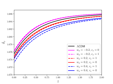
Figure 2: Collapse threshold as a function of redshift for various combinations of $w_{a}$ and $c_{s}$ indicted in the plot legend. For all models, we set $w_{0}=-1$ and $\Omega_{m0}=0.3$. As can be seen, the impact of $w_{a}$ and CDE in this quantity is very small, below $1\%$ for the examples shown in this plot.

6.2 Virialization threshold, $\delta_{{\rm v}}$

It is important to note that, implicitly in the determination of $\delta_{c}$ just described lies the assumption that DE fluctuations are not directly included in the quantities that define the collapse time and density threshold, namely $\delta^{NL}_{m}$ and $\delta^{L}_{m}$. In the $\Lambda$CDM model, baryon and dark matter fluctuations are the only relevant ones, besides a small contribution of massive neutrinos . Thus, the gravitational potential, which, for instance, will deflect light rays of background galaxies or set up the potential well that traps the hot intracluster gas, is entirely determined by the fluctuations in dark matter and baryon components. In the presence of DE fluctuations, the gravitational potential also depends on this new type of inhomogeneity. Therefore, it would be natural to redefine the threshold density, virial overdensity and growth function to take the contribution of DE fluctuations into account properly. For instance, equations (68) already suggests that the effective mass inside a shell of radius $R$ includes DE fluctuations.

Then let us define effective quantities that include DE fluctuations. The total mass inside a shell of radius $R$ is given by

$$M_{{\rm tot}}=M_{m}+M_{de}\,,$$ (73)

where $M_{de}=\frac{4\pi}{3}R^{3}\bar{\rho}_{de}\delta_{de}$. Usually the background density of DE is not included in this mass definition, e.g, Creminelli et al. (2009); Basse et al. (2012); Batista and Marra (2017). In the case of CDE, its local EoS parameter

$$w_{c}=\frac{p_{de}}{\rho_{de}}=\frac{w}{1+\delta_{de}}$$ (74)

gets less negative during the collapse. Consequently, locally, DE becomes more similar to pressureless matter, Mota and van de Bruck (2004); Abramo et al. (2008). Such variations of the EoS may also be associated with soft-matter properties Saridakis (2021).

The fraction of DE mass in the halo at the virialization time is

$$\epsilon=\frac{M_{de}}{M_{m}}\,.$$ (75)

Some authors have computed the values of $\epsilon$ with slightly different approaches to determine the virialization time, Creminelli et al. (2010); Basse et al. (2011); Batista and Pace (2013); Batista and Marra (2017); Heneka et al. (2018). In particular, using the approach summarized in equation (78), which assumes that CDE fluctuations behave as nonrelativistic particles, Batista and Marra (2017) showed that $|\epsilon|$ can be up to $0.1$, depending on $w$. In the case of phantom DE, this contribution is negative and positive for non-phantom. These values of $\epsilon$ raise an interesting question: if CDE can contribute up to $10\%$ to the total halo mass, why its impact on the critical threshold is below $1\%$?

One can also account for DE energy fluctuations in the density contrast, defined by

$$\delta_{{\rm tot}}\left(z\right)=\delta_{m}\left(z\right)+\frac{\Omega_{de}\left(z\right)}{\Omega_{m}\left(z\right)}\delta_{de}\left(z\right)\,.$$ (76)

This quantity was also used in nonlinear perturbation theory studies of CDE by Sefusatti and Vernizzi (2011). When defining the growth function as

$$D_{{\rm tot}}\left(z\right)=\frac{\delta_{tot}^{L}\left(z\right)}{\delta_{tot}^{L}\left(0\right)}\,,$$ (77)

the change between clustering and homogeneous DE models with the same background can be about $3-7\%$, while the usual definition with $\delta_{m}$ only differs about $1\%$ Batista and Marra (2017). Moreover, this work showed that the $D_{tot}$ and $D_{m}\left(1+\epsilon\right)$, where $D_{m}$ includes only the matter perturbation, are very similar, indicating consistency between the linear and nonlinear impact of CDE when using total quantities.

It is important to note that, due to the DE contribution, the total mass inside the shell is not conserved during the evolution. After virialization, however, it has been argued that this contribution should be stable Creminelli et al. (2010). In Basse et al. (2012), this effect was taken into account in the virial theorem for non-relativistic particles, yielding the following equation for virialization

$$\frac{1}{2M_{{\rm tot}}}\frac{d^{2}M_{{\rm tot}}}{dt^{2}}+\frac{2}{M_{{\rm tot}}R}\frac{dM_{{\rm tot}}}{dt}\frac{dR}{dt}+\frac{1}{R^{2}}\left(\frac{dR}{dt}\right)^{2}+\frac{1}{R}\frac{d^{2}R}{dt^{2}}=0\,.$$ (78)

Once the equations of the SCM are solved and $\delta^{NL}_{m}\left(z\right)$ and $\delta^{NL}_{de}\left(z\right)$ are known, the virialization time is determined when (78) is satisfied. For further discussion about virialization in the presence of DE, see Maor and Lahav (2005), and for relativistic corrections in the virialization, Meyer et al. (2012).

Having found the virialization redshift, one can compute the virialization threshold, including the contribution of DE fluctuations

$$\delta_{{\rm v}}\left(z_{v}\right)=\delta_{{\rm tot}}^{L}\left(z_{{\rm v}}\right)\,.$$ (79)

As can be seen in figure 3, the impact of CDE is larger than in $\delta_{c}$, reaching up to $4\%$. It is interesting to note that the magnitude of these differences is more consistent with the amount of DE fluctuations in halos described by $\varepsilon$ than those observed in $\delta_{c}$.

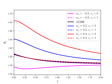
Figure 3: Virialization threshold, $\delta_{{\rm v}}$, for homogenous and CDE models with $w_{0}=-1$, $\Omega_{m0}=0.3$, and different values of $w_{a}$ and $c_{s}$ indicated in the legend. The black solid line represents the $\Lambda$CDM values and is barely distinguishable from the cases with homogeneousDE.

It is also important to highlight the behaviour of DE fluctuations. In figure 4, we show $\delta_{de}^{NL}\left(z_{v}\right)$. As can be seen, DE fluctuation can become nonlinear and have a mild decay at low-$z$, when the EoS of our examples approach $-1$. Clearly, the larger is $|w_{a}|$, more significant are the DE fluctuations. We can also see in this plot the pathological case of $\delta^{NL}_{de}<-1$ for phantom DE.

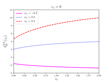
Figure 4: Nonlinear DE fluctuation in the clustering case as a function of the virialization redshift for three values of $w_{a}$ shown in the plot legend, $w_{0}=-1$ and $\Omega_{m0}=0.3$ for all models. Note that, for $w_{a}=-0.2$ we have the pathological values $\delta^{NL}_{de}<-1$.

In the presence of CDE, the virialization overdensity, defined in (44), is given by

$$\Delta_{{\rm v}}\left(z_{{\rm v}}\right)=\Omega_{m}\left(z_{{\rm v}}\right)\left[1+\delta_{m}^{NL}\left(z_{{\rm v}}\right)\right]+\Omega_{de}\left(z_{{\rm v}}\right)\delta_{de}^{NL}\left(z_{{\rm v}}\right)\,.$$ (80)

In figure 5 we show the relative difference of $\Delta_{{\rm v}}$ with respect to the $\Lambda$CDM one. Note that CDE makes $\Delta_{{\rm v}}$ more similar to the $\Lambda$CDM values.

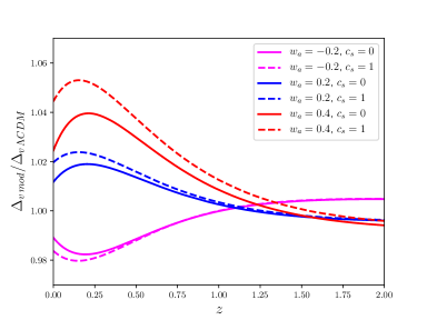
Figure 5: Ratio of $\Delta_{{\rm v}}$ of a given model indicated in the legend to the corresponding $\Lambda$CDM value. In these examples, $w_{0}=-1$ and $\Omega_{m0}=0.3$ are assumed.

7 Halo mass functions

Now let us see how to use the findings of the SCM to estimate the observational impact of DE fluctuations on structure formation. The computation of the abundance of galaxy clusters relies on the Halo Mass Function (HMF), which gives the number density of halos per comoving volume. There are several developments for the HFM, including an analytic model based on the spherical collapse by Press and Schechter (1974) and a semi-analytic approach based on ellipsoidal collapse Sheth and Tormen (1999). More recently, N-body numerical simulations were used to determine fitting functions for the HMF, e.g., Warren et al. (2006); Tinker et al. (2008). Besides determining the abundance of galaxy clusters, the HMF can be used to compute the nonlinear power spectrum, Cooray and Sheth (2002).

The proper approach to study the impact of CDE on the abundance of galaxy clusters would be to include its dynamical effects in the numerical simulations of structure formation. Codes with this capability have been developed only quite recently, but without determining the associated HMF. Let us first discuss developments based on analytic and semi-analytic HMF and then some relevant results from simulations.

We anticipate that there is no consensus of how to implement the impact of CDE in HMF. As a consequence, the predictions also vary, and the dection of DE fluctuations also depend on the particular implementation used to include the effects of CDE on halo abundances.

The Press-Schechter (PS) HMF Press and Schechter (1974) assumes that the matter density field, $\delta$, smoothed on some scale, has a Gaussian probability distribution

$$p\left(\delta\right)=\frac{1}{\sqrt{2\pi}\sigma}\exp\left(-\frac{\delta^{2}}{2\sigma^{2}}\right)\,,$$ (81)

The variance of the smoothed field, is given by

$$\sigma^{2}\left(R\right)=\int\frac{dk}{k}\frac{k^{3}P\left(k\right)}{2\pi^{2}}|W\left(kR\right)|\,,$$ (82)

where $P\left(k\right)=|\delta_{k}|^{2}$ is the linear matter power spectrum,

$$W\left(kR\right)=\frac{3}{\left(kR\right)^{3}}\left[\sin\left(kR\right)-kR\cos\left(kR\right)\right]$$ (83)

is a top-hat window function with mass-scale relation given by

$$R=\left(\frac{3M}{4\pi\bar{\rho}{}_{m0}}\right)^{1/3}$$ (84)

and $\bar{\rho}{}_{m0}$ the background matter density now.

Assuming that regions with $\delta>\delta_{c}$ form bound structures, where $\delta_{c}$ is a certain threshold value to be defined, the fraction of such objects with mass greater than $M$ is given by

$$P\left(\delta>\delta_{c}\right)=\int_{\delta_{c}}^{\infty}p\left(\delta\right)d\sigma=\frac{1}{2}\left[1-\text{erf}\left(\frac{\delta_{c}}{\sqrt{2}\sigma}\right)\right]\,.$$ (85)

The comoving number density of halos per mass interval is then given by

$$\frac{dn\left(M,z\right)}{dM}=\frac{\bar{\rho}{}_{m0}}{M}f_{PS}\left(M,z\right)\,,$$ (86)

where

$$f_{PS}\left(M,z\right)\equiv 2\left|\frac{\partial P}{\partial M}\right|\,$$ (87)

is the PS multiplicity function. The factor $2$ was first introduced in an ad hoc manner, to guarantee the normalization of the HMF Press and Schechter (1974),

$$\int_{0}^{\infty}\frac{dn\left(M,z\right)}{dM}dM=1$$ (88)

but it can be formally determined Peacock and Heavens (1990); Bond et al. (1991).

Assuming that only $\sigma$ is mass-dependent, we have the usual form of the PS multiplicity function:

$$f_{PS}\left(M,z\right)=\sqrt{\frac{2}{\pi}}\frac{1}{M}\frac{\delta_{c}\left(z\right)}{\sigma\left(M,z\right)}\left|\frac{\partial\ln\sigma\left(M,z\right)}{\partial\ln M}\right|\exp\left(-\frac{\delta_{c}^{2}\left(z\right)}{2\sigma^{2}\left(M,z\right)}\right)\,.$$ (89)

In the first studies with the PS-HMF, the values of $\delta_{c}$ assumed varied in the range $\left(1,10\right)$, e.g., Press and Schechter (1974); Efstathiou et al. (1979); Colafrancesco et al. (1989); Gelb and Bertschinger (1994). Later, it became usual to use the constant EdS collapse threshold value $\delta_{c}\simeq 1.69$, e.g., Narayan and White (1988); Peacock and Heavens (1990). In the presence of $\Lambda$ (for open, flat and closed models) Lilje (1992) reported $1.64<\delta_{c}<1.73$ at low-$z$. As we saw in subsection (4.2), other works also determined fitting functions for these quantities for homogeneous DE models Kitayama and Suto (1996); Weinberg and Kamionkowski (2003), also finding a small deviation from the EdS value, of less than $1\%$.

The matter power spectrum can be numerically determined by codes like CAMB Lewis et al. (2000) or CLASS Lesgourgues (2011). It can also be given by fitting functions, which, in most cases, can be separated in the following form

$$P\left(k\right)=P_{p}\left(k\right)T^{2}\left(k\right)D_{m}^{2}\left(z\right)\,,$$ (90)

where $P_{p}\left(k\right)$ is the primordial power spectrum associated to matter perturbations given by the inflationary model, $T\left(k\right)$ is the transfer function (for instance, given by Eisenstein and Hu (1998)) and

$$D_{m}\left(z\right)=\frac{\delta_{m}\left(z\right)}{\delta_{m}\left(z=0\right)}$$ (91)

the linear growth function of matter perturbations. Since the amount of DE is very small around the recombination time, the transfer function is essentially unaffected by DE. The main impact of DE, either smooth or inhomogeneous, is on the growth function, which strongly depends on the cosmological evolution at low-$z$.

In this context, for homogeneous DE models, the only relevant modification on the HMF occurs via the modifications on the growth function caused by different evolutions of $w$. Then it is expected that either analytic or numerical HMF can directly incorporate the impact of DE via the modifications of the growth function. Several works have studied homogeneous DE in such scenario, either with analytic approaches Percival (2005); Le Delliou (2006); Horellou and Berge (2005); Liberato and Rosenfeld (2006); Bartelmann et al. (2006); Pace et al. (2010, 2012) or numerical simulations Linder and Jenkins (2003); Grossi and Springel (2009).

For DE models with arbitrary $c_{s}$, both $\delta_{c}$ and $D_{m}$ become mass-dependent because DE fluctuations are enhanced above the sound horizon scale, and impact matter perturbations in a scale-dependent manner. This case is studied in Basse et al. (2011, 2012, 2014). Given that $\delta_{c}\left(z\right)\rightarrow\delta_{c}\left(M,z\right)$, the PS multiplicity function acquires an extra mass-dependent term

$$f_{PS}\left(M,z\right)=\sqrt{\frac{2}{\pi}}\frac{1}{M}\frac{\delta_{c}\left(M,z\right)}{\sigma\left(M,z\right)}\left|\frac{\partial\ln\sigma\left(M,z\right)}{\partial\ln M}-\frac{\partial\ln\delta_{c}\left(M,z\right)}{\partial\ln M}\right|\exp\left(-\frac{\delta_{c}^{2}\left(M,z\right)}{2\sigma^{2}\left(M,z\right)}\right)\,.$$ (92)

Although this new mass dependence is a feature of CDE if $c_{s}$ is associated with some mass scale that can be probed by the observed abundance of galaxy clusters, it is much smaller than the mass dependence on $\sigma$.

In the limit of CDE, $c_{s}\rightarrow 0$, the growth of $\delta_{de}$ has the same scale dependence of matter perturbations. Then both $\delta_{c}$ and $D_{m}$ remain scale independent. In this case, the scale dependent feature due to CDE in the HMF vanishes, but its impact can be larger. Several papers have studied this scenario: Nunes and Mota (2006); Manera and Mota (2006); Abramo et al. (2007, 2009); Creminelli et al. (2010); Batista and Pace (2013); Pace et al. (2014); Batista and Marra (2017); Heneka et al. (2018).

Now let us consider the Sheth-Tormen HMF Sheth and Tormen (1999) and how it can be modified to include the effects of DE fluctuations. Since it provides a better description of cluster abundances given by numerical simulations, we expect it to provide better estimates of the impact of DE fluctuations on clusters abundances. The original ST-HMF is given by

$$\frac{dn_{ST}}{dM}=-A\sqrt{\frac{2a}{\pi}}\left[1+\left(\frac{a\delta_{c}^{2}\left(z\right)}{\sigma^{2}\left(M,z\right)}\right)^{-p}\right]\frac{\rho_{m0}}{M^{2}}\frac{\delta_{c}\left(z\right)}{\sigma\left(M,z\right)}\frac{\partial\ln\sigma\left(M,z\right)}{\partial\ln M}\exp\left(-\frac{a\delta_{c}^{2}\left(z\right)}{2\sigma^{2}\left(M,z\right)}\right)$$ (93)

$A=0.2162$, $p=0.3$ and $a=0.707$. As in the case of PS theory, it is usual to use $\delta_{c}\simeq 1.69$. Interestingly, in the context of EdS model, the parameter $a$ reduces the effective threshold $\delta_{c\,{\rm eff}}=\sqrt{a}\delta_{c}\simeq 1.42$, indicating that $\delta_{{\rm v}}\simeq 1.52$, (45), gives a better description than $\delta_{c}\simeq 1.69$. This fact can be interpreted as an indication that the spherical collapse quantities defined at virialization time provide a more natural description of the threshold and virialization density.

Despali et al. (2016) have used several overdensities criteria to detect halos in simulations and fit the three parameters of ST-HMF. It was found that when halos are identified with the viral overdensity $\Delta_{cc}$, defined in (43), the ST-HMF is nearly universal with respect to redshift and $\Omega_{m0}$ variations. These parameters can also be constrained by future observations, see Castro et al. (2016).

Following these ideas, Batista and Marra (2017) proposed that the proper threshold density for halo formation in the presence of CDE should be modified to include the contribution of DE fluctuations at virialization time, and used virial threshold, (45). But, in order to make a more conservative estimate, the usual parameter $a$ was rescaled by $a\rightarrow\tilde{a}=a\delta_{c}^{2}/\delta_{{\rm v}}^{2}$. With this choice, the ST-HMF is unchanged in the EdS limit. In figure 3, the evolution of $\delta_{{\rm v}}$ is shown for some homogenous and CDE models.

In practice, for a given mass scale, the abundance of massive halos strongly depends on the quantities

$$\mu_{c}=\frac{\delta_{c}\left(z\right)}{D_{{\rm m}}\left(z\right)}\text{ and }\mu_{{\rm v}}=\frac{\delta_{{\rm v}}\left(z\right)}{D_{{\rm tot}}\left(z\right)}\,.$$ (94)

In figure 6 we show the ratio of these functions with respect to the corresponding values in the $\Lambda$CDM model. The impact of CDE is larger in $\mu_{{\rm v}}$ and is nearly constant with redshift-dependent. Having in mind that, although $\delta_{de}\left(z\right)$ decays at lower $z$, when $w\rightarrow-1$, the quantity $\delta_{de}\left(z\right)\Omega_{de}\left(z\right)/\Omega_{m}\left(z\right)$, which impacts both $\delta_{{\rm v}}$ and $D_{tot}$, is nearly constant. Thus, the behaviour of $\nu_{{\rm v}}$ seems more consistent with the effective contribution of DE fluctuation in the dynamics of the collapse shown in figure (4).

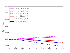
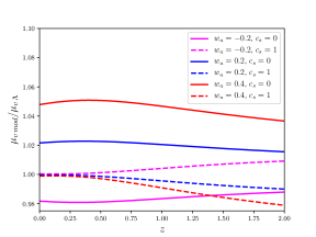
Figure 6: Evolution of $\mu_{c}$ (left panel) and $\mu_{{\rm v}}$ (right panel) with redshift, defined in equation (94), divided by the corresponding function in the $\Lambda$CDM model for homogenous and CDE models with $w_{0}=-1$ and different values $w_{a}$ and $c_{s}$ indicated in the legends. Due to the small impact of distinct DE models on $\delta_{c}$, the differences in $\mu_{c}$ with respect to the case with $\Lambda$ is very small at $z\simeq 0$, but can reach about $2\%$ at $z\simeq 2$. In the case of CDE, the differences in $\mu_{{\rm v}}$ are larger and also present at low $z$.

Another important point regarding the impact of CDE on HMFs is that they are not calibrated by numerical simulations. A possible approach to this issue, also used in the context of non-gaussianities LoVerde et al. (2008) and baryonic feedback Velliscig et al. (2014), is to multiply the more accurate numerically calibrated HMF by a factor that encodes the relative impact of DE fluctuations with respect to the usual homogeneous model Creminelli et al. (2010); Batista and Marra (2017); Heneka et al. (2018)

$$\frac{\left(dn/dM\right)_{c_{s}=0}}{\left(dn/dM\right)_{c_{s}=1}}\,.$$ (95)

Moreover, one has to take into account how CDE affects the cluster mass. It is expected that the contribution of DE to mass shifts HMF according to $M\rightarrow M\left(1-\epsilon\right)$ Creminelli et al. (2010); Batista and Pace (2013); Batista and Marra (2017). Batista and Marra (2017) also analyzed modifications on the mass-scale relation, equation (84), and normalization condition. Whereas the former can be safely neglected, the latter is of the order of $\epsilon$, possibly modifying HMF about a few per cent on all mass scales. These studies have shown that, depending on the evolution of $w$, the abundance of massive halos can change by $10-30\%$ with respect to homogeneous DE models. But this change can be even larger very massive halos, $M>10^{15}M_{\odot}$, whose abundance is very sensitive to modifications on the exponential tail of HMF.

Numerical simulations

Recently, numerical simulations capable of treating CDE were developed. The first approach proposed was to include DE linear perturbations given by Einstein-Boltzmann solvers as a new source of the gravitational potential in N-Body simulations Dakin et al. (2019). Of course, this implementation can not deal with nonlinear DE fluctuations, but was crucial in confirming that linear and mildly nonlinear DE perturbations have a non-negligible impact on structure formation.

Hassani et al. (2019) developed a code capable of describing nonlinear DE fluctuations. They showed that models with $w=-0.9$ and $c_{s}=10^{-3.5}$ do impact matter fluctuations and the gravitational potential on small scales. They also found that DE and matter fluctuations are correlated, as indicates the solution (14). However, HMF was not computed. Hassani et al. (2020) also studied the imprint of CDE on observables associated with the gravitational potential. They confirmed the tendency of CDE to compensate for the changes in the background and found modifications of $2-5\%$ on the observables studied. It is important to note that, due to the choice $w=-0.9$, the imprints of DE fluctuations found in these works are not as large as in models in which $w$ is smaller at intermediate redshifts.

Although these numerical studies have confirmed several results from perturbation theory and the SCM, the distinct proposals to implement the impact of CDE on HMF were not yet tested by simulations. Unfortunately the results vary between these implementations, and there is no definitive prediction about the actual impact of CDE on the abundance of galaxy clusters. See also the discussion in Basse et al. (2014)

8 Cosmological observables

As we saw, DE fluctuations can potentially impact the linear and nonlinear evolution of matter fluctuations and the gravitational potential. Thus, many observables like CMB anisotropies, linear and nonlinear matter power spectrum and growth rate can change due to the presence of a new clustering component. We have already discussed some of those effects, especially regarding HMF. Next, overview of some observational strategies discussed in the literature that can possibly detect CDE. The grouping of observables shown below is somewhat arbitrary because most of the works presented discuss and analyze combinations of them.

8.1 CMB and Large Scale Structure

Weller and Lewis (2003) attempted to constrain the value of $c_{s}$ using the first WMAP data release and found that $c_{s}$ is unconstrained. In a similar analysis, Bean and Dore (2004) reported a $1\sigma$ constraint $c_{s}<0.2$. Later, Hannestad (2005) included Large Scale Structure data in the analysis, showing that $c_{s}$ remains essentially unconstrained. de Putter et al. (2010) also reached the same conclusion, but showing that chances of detection of CDE are larger in Early DE models.

Takada (2006) showed that a $2000$$\text{deg}^{2}$ galaxy redshift survey at $z\simeq 1$, together with CMB information from Planck, can distinguish between smooth ($c_{s}=1$) and CDE with $c_{s}<0.02$ and $w=-0.95$.

Analyzing Early DE models and using CMB and LSS data, Bhattacharyya and Pal (2019) reported $c_{s}=0.37$ and $\Omega_{de}\left(a_{rec}\right)=0.02$. It was shown that, when $c_{s}$ is allowed to vary, the contribution of DE in the early Universe can be more significant.

It has also been shown that the cross-correlation between galaxy survey and the Integrated Sachs-Wolf effect is a promising technique to detect $c_{s}$ Hu and Scranton (2004). This idea was further explored in Corasaniti et al. (2005); Pietrobon et al. (2006); Ballesteros and Lesgourgues (2010); Li and Xia (2010).

The most recent analysis of CDE by the Planck team Ade et al. (2016) indicates that $c_{s}$ is unconstrained. However, $w$ was assumed constant. Since at late times we must have $w\simeq-1$, DE fluctuations are very small in this scenario, and the impact of $c_{s}$ on observables is negligible. Only models with time-varying $w$ can present relevant DE fluctuations, like in the case o Early DE.

8.2 Higher order perturbation theory

CDE has also been studied in the framework of higher-order perturbation theory by Sefusatti and Vernizzi (2011); D’Amico and Sefusatti (2011); Anselmi et al. (2011, 2014). These works found an impact of a few per cent on nonlinear corrections to the linear power spectrum. These authors also understand that, in CDE models, the total perturbation is the relevant one to be considered, not only matter perturbations.

8.3 Weak lensing

Sapone et al. (2010) investigated how tomographic weak lensing and galaxy redshift surveys can constrain DE sound speed. Considering $w=-0.8$ they found that, if $c_{s}<0.01$, the sound speed can be constrained. More studies in this direction include Ayaita et al. (2012); Majerotto et al. (2016)

8.4 Cluster abundances

Abramo et al. (2009) have forecasted the constraining power of galaxy clusters surveys on $c_{s}$. Although the implementation used is not entirely consistent with SCM in the sense of how $c_{s}$ is varied, what artificially enhances the dependence of cluster abundances on this parameter, some interesting conclusions were drawn. It was shown that future experiments like Euclid can play a decisive role in detecting DE fluctuations and that they impact the constraints on $w_{0}$ and $w_{a}$ at $10-30\%$ level.

Basse et al. (2014) has also forecasted how $c_{s}$ can be constrained by data from cluster abundances, CMB, cosmic shear and galaxy clustering correlations. It was found that, considering $w_{0}=-0.83$ and $w_{a}=0$, future Euclid data can distinguish between $c_{s}=1$ and $c_{s}=0$. However, this result strongly depends on how the impact of CDE is implemented on HMF. In particular, it was found that, when considering the DE contribution to the cluster mass, the sensitivity on $c_{s}$ significantly degrades.

Appleby et al. (2013) showed that, using the Euclid satellite cluster survey together with Planck data, Early DE models with $c_{s}<0.1$ and $\Omega_{de}\left(a_{{\rm rec}}\right)=0.009$ can be distinguished from models with $c_{s}=1$. In such models, DE is not negligible at high-$z$ and the EoS parameter can be larger than $-1$ at high-$z$. Hence, the impact of DE perturbations is strongly enhanced. The authors noted that $c_{s}$ is mainly constrained by CMB data. Although this work used the Tinker HMF Tinker et al. (2008), which does not take into account the nonlinear effects of DE fluctuations, the reported insensitiveness of cluster abundance on clustering Early DE model is in accordance with Batista and Pace (2013). The reason for this is the following: whereas Early DE has a strong impact on the background evolution, decreasing the matter growth, if it clusters, the perturbations partially compensate for this change. Note, however, that this result was obtained using $\delta_{c}$ and $D_{m}$. When using $\delta_{{\rm v}}$ and $D_{{\rm tot}}$ in HMF, it is expected that more pronounced changes due to CDE will be present.

Heneka et al. (2018) used cluster data from several experiments plus CMB, Barion Acoustic Oscillations (BAO) and Supernova Ia (SNIa) observations to constraint cosmological parameters with $c_{s}=1$, $c_{s}=0$ and constant $w$. It was shown that the allowed regions in the $\sigma_{8}-\Omega_{m0}$ plane change due to CDE. It was found that $w<-1$ is preferred by data and that $\sigma_{8}$ is reduced when $c_{s}=0$. This impact of CDE can alleviate the tension in cluster data found by Planck Ade et al. (2015).

It is important to note that, a possible issue regarding constraints of CDE models with cluster data is associated with the observable-mass scaling relations, see Mantz et al. (2010); Kravtsov and Borgani (2012). So far, no analytical or numerical study has been conducted to explore the impact of DE fluctuation on these relations. As discussed before, DE fluctuations certainly impact the gravitational potential, thus lensing signals, X-ray can SZ luminosities relations with the cluster mass can be affected.

8.5 Internal structure of galaxy clusters

The impact of CDE on the internal structure of halos was studied in Mota (2008); Basilakos et al. (2009). As it would be expected from the results that $R_{{\rm ta}}/R_{{\rm v}}<0.5$ in the presence of DE and its possible perturbations, the concentration parameter of galaxies clusters increases. Basilakos et al. (2009) have analyzed the mass-concentration relation of four massive clusters, showing that the data is better described by CDE models.

8.6 $S_{8}$ tension and growth rate

Clustering DE models can be used to reduce the value of $\sigma_{8}$, Kunz et al. (2015). The parameter $S_{8}=\sigma_{8}\sqrt{\Omega_{m0}/0.3}$ inferred by CMB observations using the $\Lambda$CDM model, Aghanim et al. (2020), is about $3\sigma$ in tension with the values determined by weak lensing observations Asgari et al. (2021); Abbott et al. (2021), see also Di Valentino et al. (2021) and references therein. To explore the impact of CDE – here we will focus on the variation of $\sigma_{8}$ only – we fix $\sigma_{8mod}\left(z\right)=\sigma_{8mod}D_{mod}\left(z\right)$, for a given model "$mod$", to have the same value as in the $\Lambda$CDM model at $z_{rec}$

$$\sigma_{8mod}=\frac{D_{\Lambda}\left(z_{rec}\right)}{D_{mod}\left(z_{rec}\right)}\sigma_{8\Lambda}\,,$$ (96)

where $\sigma_{8\Lambda}=0.8111$ for $\Omega_{m0}=0.3153$ Aghanim et al. (2020).

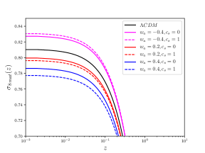
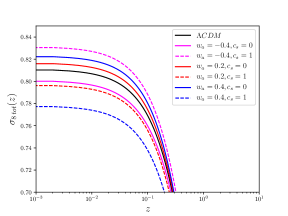
Figure 7: Redshift evolution of $\sigma_{8}\left(z\right)$ for various DE models indicated in the legends. In the left panel: the growth function is given only by the matter perturbation. Right panel: the growth function is computed including the CDE contribution given by (76).

As can be seen in the left panel of figure (7), in the case where only matter perturbations contribute to the growth function, CDE make the evolution of $\sigma_{8}\left(z\right)$ more similar to $\Lambda$CDM. In the right panel, when DE perturbations are included in the growth function, we see that the impact of CDE is much larger. In this case, for $w_{a}>0$ ($w_{a}<0$), DE perturbations can make $\sigma_{8}\left(z\right)$ larger (smaller) than in $\Lambda$CDM.

Homogeneous phantom DE increase $\sigma_{8}$ because $\Omega_{de}\left(z\right)$ grows rapidly at low-$z$, delaying the suppression of matter perturbations when compared to $\Lambda$CDM. When DE perturbations are allowed, given that $\delta_{de}<0$, matter growth is suppressed. Considering the total growth function, this effect can potentially alleviate the $S_{8}$ tension.

On the other hand, homogeneous non-phantom DE decrease $\sigma_{8}$ because $\Omega_{de}\left(z\right)$ starts to grow earlier than in $\Lambda$CDM model. Clustering DE now partially compensates for this decay in the growth of matter perturbations, enhancing $\sigma_{8}$. For the case of the total growth function, CDE can potentially worsen the $S_{8}$ tension.

An analysis of CDE using cluster, CMB, BAO and SNIa data was done by Heneka et al. (2018). It was found the $\sigma_{8}$ is reduced for $c_{s}=0$ with slight increase in $\Omega_{m0}$. Considering the best fit values, the overall effect is a reduction of $S_{8}$ in CDE models. The results also show that, assuming constant $w$, phantom values are prefered by data.

Clustering DE also affects the growth rate of matter Batista (2014); Mehrabi et al. (2015a, b), given by

$$f\left(z\right)=\frac{d\ln\delta_{m}}{d\ln a}\,$$ (97)

In particular, Mehrabi et al. (2015c) reported that CDE models can fit $f\left(z\right)\sigma_{8}\left(z\right)$ data better than $\Lambda$CDM.

9 Discussion

The variety of models that try to explain the cosmic acceleration is enormous. The most studied and tested ones either do not present DE fluctuations ($\Lambda)$ or have negligible fluctuations on scales well below the horizon (quintessence). However, many other models can present a low $c_{s}$ value and relevant DE fluctuations on small scales. However, the actual amount of DE fluctuations also depends on the evolution of EoS. If $w\simeq-1$ throughout the cosmic evolution, DE fluctuations are very small, regardless of the value of $c_{s}$.

Hence, the prospects to detect DE fluctuations on small scales, which would rule out $\Lambda$ and quintessence as possible drivers of cosmic acceleration, strongly depend on how far from $-1$ the EoS can be in the past. Although $\Lambda$ is in excellent agreement with almost all cosmological data available, there are no strong constraints on how much $w$ can deviate from $-1$ at intermediate redshifts. For instance, the allowed parameter space for $w_{0}$ and $w_{a}$ for the case of $c_{s}=1$ is still very large Ade et al. (2016). As we reviewed, for constant EoS, DE models with $w\simeq-0.9$ and $c_{s}<10^{-2}$ leave a detectable impact on several cosmological observables. Being more conservative with the value of $w$ now, we showed that, even with $w_{0}=-1$, DE fluctuations become nonlinear when assuming $|w_{a}|>0.2$ and $c_{s}=0$, and influence structure formation.

The linear evolution and the corresponding impact of DE perturbations is well understood and implemented in numerical codes like CAMB and CLASS. The nonlinear evolution in the presence of CDE is, however, more complicated and much less developed. First efforts in this direction used the SCM and only recently numerical codes for the nonlinear evolution were developed. The early findings about the phenomenology of CDE are in agreement with those found by recent numerical results. These studies have shown that DE fluctuations can become nonlinear and do impact matter fluctuations, the formation of halos and the gravitational potential.

The abundance of massive galaxy clusters is certainly one of the most affected observables. However, up to now, no numerical simulations modelled the impact of CDE in HMF. The analytical motivated proposals for HMF in the presence of CDM are divided into two main groups: one in which the impact of CDE enters only via the matter quantities ($\delta_{c}$, $D_{m}$, $\sigma_{8m}$) and another based on the total weighted fluctuations ($\delta_{{\rm v}}$, $D_{{\rm tot}}$, $\sigma_{8{\rm tot}}$). Naturally, the impact of CDE is enhanced in the latter type of modifications. Moreover, these different recipes can be combined with mass rescalings due to DE contribution, $M\rightarrow M\left(1+\epsilon\right)$. However, there is no consensus on the literature on which is the accurate implementation to compute the effect of CDE on halo abundances.

An important theoretical issue with CDE models is associated with phantom models. For $c_{s}\rightarrow 0$, one can have $\delta_{de}<-1$ in the nonlinear regime. At first glance, this indicates that these models are inconsistent. A possible realization of phantom clustering models may include imperfect fluids Sawicki et al. (2013).

Although CDE is the natural minimal generalization to quintessence, it is still not well explored in the literature. Studies which consider parametrizations of $w$ are very common, but rarely consider $c_{s}<1$. As discussed, CDE can play a role in alleviating the $S_{8}$ tension. From another perspective, there is no indication that DE can not present relevant fluctuations on small scales. Therefore, these kinds of models deserve more attention from the cosmology community.

Besides these difficulties, preliminary forecasts studies indicate that future experiments like Euclid will be able to discriminate between homogeneous and CDE. The challenges to achieve this goal are big. Most of the constraining power of Euclid will come from nonlinear scales, and a good understanding of the nonlinear effects of CDE will be mandatory.