The GAPS programme at TNG ^,

Abstract

Context. Active region evolution plays an important role in the generation and variability of magnetic fields on the surface of lower main-sequence stars. However, determining the lifetime of active region growth and decay as well as their evolution is a complex task. Most previous studies of this phenomenon are based on optical light curves, while little is known about the chromosphere and the transition region.

Aims. We aim to test whether the lifetime for active region evolution shows any dependency on the stellar parameters, specially on the stellar age.

Methods. We identify a sample of stars with well-defined ages via their kinematics and membership to young stellar associations and moving groups. We made use of high-resolution échelle spectra from HARPS at La Silla 3.6m-telescope and HARPS-N at TNG to compute rotational velocities, activity levels, and emission excesses. We use these data to revisit the activity-rotation-age relationship. The time-series of the main optical activity indicators, namely Ca ii H & K, Balmer lines, Na i D₁, D₂, and He i D₃, were analysed together with the available photometry by using state-of-the-art Gaussian processes to model the stellar activity of these stars. Autocorrelation functions of the available photometry were also analysed. We use the derived lifetimes for active region evolution to search for correlations with the stellar age, the spectral type, and the level of activity. We also use the pooled variance technique to characterise the activity behaviour of our targets.

Results. Our analysis confirms the decline of activity and rotation as the star ages. We also confirm that the rotation rate decays with age more slowly for cooler stars and that, for a given age, cooler stars show higher levels of activity. We show that F- and G-type young stars also depart from the inactive stars in the flux-flux relationship. The gaussian process analysis of the different activity indicators does not seem to provide any useful information on active region’s lifetime and evolution. On the other hand, active region’s lifetimes derived from the light-curve analysis might correlate with the stellar age and temperature.

Conclusions. Although we caution the small number statistics, our results suggest that active regions seem to live longer on younger, cooler, and more active stars.

1 Introduction

The relationships among stellar activity, rotation, and stellar age in solar-type stars have been widely studied. Chromospheric activity and rotation are linked by the stellar dynamo and as the star evolves during the main-sequence phase loosing angular momentum via magnetic braking, both rotation and activity diminish (e.g. Schatzman, 1962; Kraft, 1967; Weber & Davis, 1967; Skumanich, 1972; Noyes et al., 1984; Kawaler, 1989; Soderblom et al., 1991; Jianke & Collier Cameron, 1993; Montesinos et al., 2001; Barnes, 2007; Mamajek & Hillenbrand, 2008).

Active region (hereafter AR) growth and decay is another phenomenon related to the surface magnetic activity of solar-type stars with convective outer layers. The study of AR is fundamental to improve our knowledge about the generation of magnetic fields and their variability. However, there are few works dealing with the analysis of AR lifetimes. In a series of papers, Donahue et al. (1997a, b) use the pooled variance technique on calcium data to infer the AR lifetimes of approximately one hundred of lower main-sequence stars. The authors show that AR have rather irregular lifetimes and that different stars might show very different pooled variance diagrams depending on their level of activity (age), and colour (mass).

More recently, several works have developed a methodology based on the decay of the autocorrelation function of light curves (in particular using data from the Kepler mission) to put constraints on the spot and AR lifetime. Giles et al. (2017) find that big starspots live longer irrespective of the spectral type of the star and that starspots decay more slowly on cooler stars. Santos et al. (2021) and Basri et al. (2022) discuss the effect of differential rotation and how it can destroy the biggest ARs leading to a shorter AR lifetime. It is important to note that these works are based on optical light curves and therefore their conclusions refer to the ARs evolution in the stellar photosphere. However, it is well known that solar AR in the chromosphere and in the transition region have lifetimes 4-5 times longer than the ARs in the solar photosphere.

Therefore, a detailed and homogeneous analysis of the chromospheric activity indexes of a large sample of stars with reliable age estimates is needed before possible mechanisms for AR growth and decay are invoked. This is the goal of this paper, in which we take advantage of the high amount of high-resolution spectra taken within the framework of current radial velocity planet searches to derive in an homogeneous way the time-series of the main optical activity indexes for a large sample of stars in open clusters and stellar associations with precise age estimates. Some of these stars have also available photometry time series from the TESS mission. We also take advantage of state-of-the-art statistical analysis to model stellar activity such as Gaussian processing.

This paper is organised as follows. We present our stellar sample in Sect. 2. Section 3 describes the analysis of the data while in Sect. 4 we use our dataset to revisit the activity, rotation, and age relationships. The dependency of AR lifetimes on spectral type, activity, and stellar age are discussed in Section 5. Our conclusions follow in Sect. 6.

2 Stellar sample

The sample analysed in this work is composed of 130 stars in open clusters or stellar associations with well known derived ages. The bulk of the sample is formed by stars observed within the framework of the Global Architecture of Planetary Systems programme (GAPS, Covino et al., 2013). In particular, 25 stars were selected from the GAPS Young Objects Project, a radial velocity survey aimed to probe the frequency of planets around young stars (Carleo et al., 2020). It includes young stars in well known star forming regions (e.g. the Taurus complex with an age of $\sim$ 2 Myr) as well as bona-fide members of open clusters and moving groups (such as Coma Ber or Ursa Major, age $\sim$ 400-600 Myr). Additional 48 stars were taken from the GAPS Open Cluster Project, a monitoring of selected stars in three open clusters (namely the Hyades, M44, and NGC 752) aimed to study the relation between the physical properties of the planets and those of their host stars as well as the connection between the physical properties of the cluster environments and those of their planetary systems. (Malavolta et al., 2016). Finally, 56 stars members of clusters and moving groups or with well-known ages were selected from Mamajek & Hillenbrand (2008, hereafter MH08). Table 1 lists the number of stars by open cluster or kinematic group, while the corresponding Hertzsprung-Russell (HR) diagram of the observed stars is shown in Fig. 1.

Table 1: Number of observed stars per cluster or moving group.

Association	N stars	Age	Ref.
		(Myr)
Taurus	4	1 - 2	(a)
Upper Sco	4	10	(b)
Cepheus	2	10 - 20	(c)
$\beta$ Pic	2	24	(d)
Tucana - Horologium	4	30	(e)
Pleiades	2	112	(f)
AB Dor	2	149	(g)
Castor	1	200	(h)
Hercules - Lyra	1	257	(i)
Ursa Major	6	414	(j)
Coma Berenices	6	562	(k)
Praesepe	20	578	(l)
Hyades	49	750	(m)
Other young stars	2	50 - 600	(n,o)
NGC 752	12	1340	(p)
Old stars	13	5300 - 13900	(q)
Sun		4579†	(r)

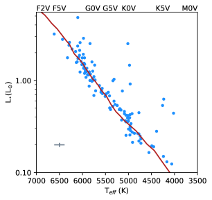
Figure 1: Luminosity versus T_eff diagram for the observed stars. The red line shows the main sequence from Pecaut & Mamajek (2013).

The stars are required to have high-resolution, HARPS-N (Cosentino et al., 2012) or HARPS (Mayor et al., 2003) optical échelle spectra. The instrumental setup of HARPS and HARPS-N is almost identical. The spectra cover the range 378-691 nm (HARPS) and 383-693 nm (HARPS-N) with a resolving power of R $\sim$ 115000. The spectra are provided already reduced using HARPS-N/ESO standard calibration pipelines (Data Reduction Software, DRS version 3.7 and 3.8 respectively ) and were retrieved from the corresponding ESO and TNG archives. In addition, several solar spectra taken by the HARPS-N solar telescope (Dumusque et al., 2021) were analysed in order to use the Sun as a benchmark.

3 Analysis

3.1 Kinematics and age

Stellar age is one of the most difficult stellar parameter to constrain in an accurate way. Solar-type stars evolve too slowly to be dated by their position in the Hertzsprung-Russell diagram. Membership to stellar associations and kinematic groups has been proposed as a way to overcome this difficulty and used as a methodology to identify young stars and to assign ages, specially after the release of the Hipparcos data. Today, the exquisite precision of the recently released Gaia EDR3 catalogue (Gaia Collaboration, 2020) allows us to compute precise Galactic spatial velocity components $(U,V,W)$ and detailed probabilities of membership to young stellar associations.

Galactic spatial velocity components were computed from the radial velocities, and Gaia parallaxes and proper motions (Gaia Collaboration, 2020) following the procedure described in Montes et al. (2001) and Maldonado et al. (2010). In brief, the original algorithm (Johnson & Soderblom, 1987) is adapted to epoch J2000 in the International Celestial Reference System (ICRS) as described in Sect. 1.5 of The Hipparcos and Tycho Catalogues’ (ESA, 1997). To take into account the possible correlation between the astrometric parameters, the full covariance matrix was used in computing the uncertainties. The corresponding $(U,V)$ plane is shown in Fig. 2.

It can be seen that most of our targets are in the region of the diagram occupied by the young stars (as expected). Only some old stars taken from the literature (see above) are outside the boundary of the young star’s region. Once young stars are identified we made use of Bayesian methods to confirm their membership to young stellar associations (BANYAN, Gagné et al., 2018).

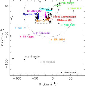
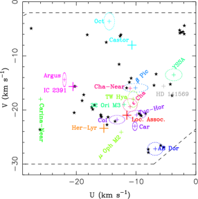
Figure 2: Left: $(U,V)$ plane showing the position of the known kinematic groups in the solar neighbourhood. Large crosses represent the convergence point of the “classical” moving groups. Coloured asterisks show the position of the so-called “old” moving groups. Our stars are shown by black filled star symbols. The dashed line represents the boundary of the young disc population as defined by Eggen (1984, 1989). The dotted line represents the velocity ellipsoid determined by Francis & Anderson (2009). Right: Zoom of the region of the $(U,V)$ plane around the Local Association.

3.2 Rotational velocity

Rotational velocities were computed by means of the Fourier Transform (FT) technique (e.g. Gray, 2008). In brief, the dominant term in the Fourier transform of the rotational profile is a first-order Bessel function that produces a series of relative minima at regularly spaced frequencies. The first zero of the Fourier transform is related to $v\sin i$ by:

$$v\sin i=\frac{c}{\lambda}\times\frac{k_{1}}{\sigma_{1}}$$ (1)

where $c$ is the speed of light, $\lambda$ is the central wavelength of the considered line, ${\sigma_{\rm 1}}$ is the position of the first zero of the Fourier Transform, and ${k_{\rm 1}}$ is a function of the limb darkening coefficient ($\epsilon$) that can be approximated by a fourth-order polynomial degree (Dravins et al., 1990)

$$k_{1}=0.610+0.062\epsilon+0.027\epsilon^{2}+0.012\epsilon^{3}+0.004\epsilon^{4}$$ (2)

where we assume $\epsilon$ = 0.6 (see e.g. Gray, 2008). Four spectral lines at 6335.33 Å, 6378.26 Å, 6380.75 Å, and 6393.61 Å were used for the computations. An additional line at 6400.11 Å was used but only for stars with high rotation values, since it is a blend of two lines that at low rotation levels are resolved. Given that it is not an isolated line, we only considered this blend if the derived $v\sin i$ value was compatible with the values obtained from the other lines.

In addition to the FT method, we fitted each line profile to a rotational profile following the prescriptions of Gray (2008). The fits were performed within a Bayesian framework based on a Monte Carlo Markov Chain (MCMC) sampling of the parameter space. Since the rotational profile does not take into account the wings of the line profile (we note that the function is not defined on those points), the profile was convolved with a Lorentzian profile. Therefore, the model contains five parameters namely, the centre of the profile, the depth of the profile, the Lorentzian parameter, the amplitude of the profile, and an additional jitter term.

A comparison of the derived $v\sin i$ values obtained by using the FT method and those derived using the line profile fitting is shown in Fig. 3 (left panel). Although the overall agreement is good, it can be seen that the line profile fitting method tends to provide slightly larger $v\sin i$ values. In particular, we note that for the Sun we obtain a mean value of 3.23 $\pm$ 0.13 kms^-1 when using the FT method, and 4.43 $\pm$ 0.26 kms^-1 from the fitting profile technique (that can be compared with the adopted value of $\sim$ 2.0 kms^-1). Fig. 3 also shows a comparison of our obtained equatorial velocities with those provided in the literature. The literature values are taken from the compilation of Glebocki & Gnacinski (2005, hereafter GL05). It can be seen that the agreement of our FT values with those from the literature is overall good (centre panel), specially at $v\sin i$ values larger than 10 kms^-1, with most stars lying close to the 1:1 relationship. At lower rotation levels, however, the scatter is larger. The residual mean square (rms) of the comparison is 1.90 kms^-1, the root-mean squared error (rmse) is 3.6 kms^-1, and the R² (coefficient of determination) is $\sim$ 0.98. When considering the values derived from the line profile fitting (right panel), we obtain larger values than those found in the literature. This effect is more pronounced at the low rotation level. In this case, we obtain an rms value of 3.40 kms^-1, with an rmse value of 11.6 kms^-1, and R² $\sim$ 0.93.

We conclude that the rotational profile fitting method works better at large rotational velocities. At low-rotation levels, however, the width of the line profiles are dominated by the intrinsic sources of line broadening such as micro and macroturbulence, pressure and magnetic Zeeman splitting. As a consequence, in low-rotation stars, the fitting method tends to overestimate the $v\sin i$ values. Therefore, in the following, we will consider only the $v\sin i$ values derived by using the FT method.

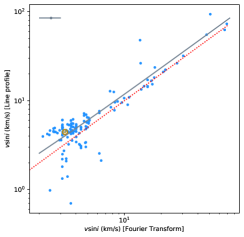
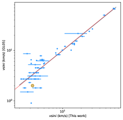
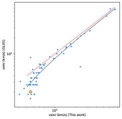
Figure 3: Left: Comparison between the $v\sin i$ derived from the fit of line profiles to a rotational profile, and $v\sin i$ derived by using the FT technique. Centre: Comparison between the mean $v\sin i$ provided by GL05 and those measured in this work using the FT technique. Right: Comparison between the mean $v\sin i$ provided by GL05 and those measured in this work by the fitting of line profiles to a rotational profile. The red dotted line shows the 1:1 relationship while the grey dashed line shows the best linear fit. The position of the Sun is shown with the symbol $\odot$. Typical error bars in GL05 data are of the order of 1.4 kms^-1.

3.3 Activity indexes

For the examination of activity indexes we use the strong optical lines Ca ii H & K, Balmer lines (from H$\alpha$ to H$\epsilon$), Na i D₁, D₂, and He i D₃. Our definition of the bandpasses for the activity indexes follows Maldonado et al. (2019, and references therein). In order to transform the measured S index into R’_HK, a mean S index was computed for each star and transformed into the Mount Wilson scale by a comparison with the stars in common with Duncan et al. (1991). The comparison is shown in Figure 4. An ordinary least squares fit was performed in order to obtain a relationship between the S index measured in this work and the S index in the Mount Wilson scale. A 3$\sigma$ clipping procedure was applied to identify outliers to the best linear fit. We note that the outliers correspond to stars for which only one measurement is available. Given their rather high S index values we speculate that these stars might have a high a level of chromospheric variability. We obtain the following relationship

$$S_{\rm MW}=(1.52\pm 0.10)\times S_{\rm tw}-(0.074\pm 0.025)$$ (3)

where S_MW is the S index in the Mount Wilson scale and S_tw is the S index as measured in this work.

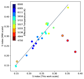
Figure 4: Activity S index in the original Mount Wilson scale as a function of the S index as measured in this work. Different colours indicate the effective temperature of the stars. Outliers are highlighted in purple circles. Errors are within the symbol dimension. The best linear fit is shown in grey.

The S index contains both the contribution of the photosphere and the chromosphere. Empirical relationships to correct for the photospheric contribution have been calibrated using the colour index (B-V). Furthermore, a conversion factor to correct for flux variations in the continuum passbands and normalise to the bolometric luminosity should be applied (Noyes et al., 1984). Unfortunately, for most of our targets there are no reliable B, V magnitudes available in the literature. Therefore, we use the Gaia DR2 (Gaia Collaboration, 2018) effective temperature to estimate the (B-V) colour of our target stars. In order to do that, we derive a (B-V)-T_eff relationship using the data by Flower (1996). Details on this calibration are given in Appendix A.

The conversion factor and photospheric corrections most widely used are those provided by Noyes et al. (1984, hereafter NO84). They are, however, only valid for solar-type stars with 0.44 $<$ (B-V) $<$ 0.82 (spectral types between F5 and K2). More recently, Suárez Mascareño et al. (2015) derived conversion factors and photospheric corrections for cooler stars (up to (B-V) = 1.9).

3.4 Rotation periods and lifetime of active regions

In order to determine the stellar rotation period from the different activity indexes and the available TESS photometric time series, we started by using the Generalised Lomb-Scargle periodogram (Zechmeister & Kürster, 2009) to identify periodic signals in the data. We then model the data using Gaussian Process regression in a Bayesian framework with the following likelihood

$$lnp({y_{n}},{t_{n}},{\sigma^{2}_{n}},\theta)=-\frac{1}{2}\textbf{r}^{T}K^{-1}\textbf{r}-\frac{1}{2}\ln{\det K}-\frac{N}{2}\ln{2\pi}$$ (4)

where $y_{n}$, $t_{n}$, $\sigma_{n}$ are, respectively, the data, time of observations and errors, $\theta$ is the array of parameters, r is the residual vector obtained by removing the model from data, $K$ is the covariance matrix and $N$ are the number of observations.

We selected the widely used Quasi-Periodic function obtained by multiplying a constant term to an exp-sin-squared kernel and to a squared-exponential kernel (george python package, e.g. Ambikasaran et al., 2015; González-Álvarez et al., 2021; Maldonado et al., 2021) and it is defined as follows

$$k(i,j)=h^{2}\exp{\left(-\frac{(t_{i}-t_{j})^{2}}{\tau^{2}}-\frac{\sin^{2}(\pi(t_{i}-t_{j})/P_{rot})}{2\omega^{2}}\right)}$$ (5)

where $k(i,j)$ is the $i$-th $j$-th element of the covariance matrix, $t_{i}$ and $t_{j}$ are two times of the data set, $h$ is the amplitude of the covariance, $\tau$ is the timescale of the exponential component, $\omega$ is the weight of the periodic component, $P_{rot}$ is the period.

We do not include an extra error term ($\sigma_{Jit}$) as the uncertainties of the measured indexes are relative large. However, we added a linear trend model ($\gamma$ + $\dot{\gamma}t$). At the beginning of the Gaussian Process regression, both data and errors have been cleaned by a (3) sigma-clip procedure. The parameter space is sampled with emcee (Foreman-Mackey et al., 2013) set with 72 walkers randomly initialised within parameter boundaries, they are reported in Table 2. We have imposed uniform priors on $P_{\rm rot}$ with boundaries according to the False Alarm Probability (FAP) of the maximum power GLS period. We used as prior boundaries P_GLS $\pm$ 1 d, P_GLS $\pm$ 3 d, P_GLS $\pm$ 8 d, and P_GLS $\pm$ 15 d for FAP $<$ 0.1%, 0.1% $<$ FAP $<$ 1%, 10% $<$ FAP $<$ 1%, and 10% $>$ FAP, respectively. We note that for the analysis of the TESS photometric data, better results were obtained in some cases by using gaussian priors centred around the known values of P_rot (see Sect. 5.4). Finally we set a conservative burn-in phase of 40K, while 10K were used to obtain the posterior distributions.

Table 2: Model priors. Labels $\mathcal{U}$ and $\mathcal{LU}$ represent uniform and log-uniform distribution, respectively, while P_GLS is the period of maximum power obtained from the GLS periodogram.

Parameter	Priors	Description
linear trend
$\gamma$	$\mathcal{U}$(min(index), max(index))	Minimum and maximum value of the index
$\dot{\gamma}$	$\mathcal{U}$(min(slope),max(slope))	Slopes of the data computed in the first/second
		half-seasons of the observations (d-1)
GP parameters
$h$	$\mathcal{L}\mathcal{U}$(10-6, 10+6)
$\tau$	$\mathcal{L}\mathcal{U}$((minimum $P_{\rm rot}$ prior)/2, 104)	(d)
$\omega$	$\mathcal{L}\mathcal{U}$(10-2,10)
$P_{\rm rot}$	$\mathcal{L}\mathcal{U}$(PGLS $\pm$ $nn$ d)	$nn$ depends on the FAP, see text (d)

4 The rotation - age - activity relationships

4.1 Rotation vs. age and spectral type

Figure 5 shows the $v\sin i$ values as a function of the stellar age. The general tendency of lower rotation rates towards older stellar ages is clearly visible. We fit the data to a power law of the form:

$$v\sin i\propto\alpha\times t^{\beta}$$ (6)

where the parameters $\alpha$ and $\beta$ are drawn from a bayesian framework using an MCMC simulation. The best-fit parameters are given in Table 3. The figure also shows a dependency of the rotation vs. age relationship on the stellar spectral type. Rotation in cooler stars shows a lower decay than in hotter stars. In order to test that, we divided our target stars into three subsamples, namely, stars hotter than 5790 K (that is, a G2-type star), stars with effective temperatures between 4800 K and 5790 K (spectral type between G2 and K2), and stars cooler than K2. The results are given in Table 3. They show that the $\beta$ parameter (the slope) is greater for stars with spectral type earlier than G2, while the constant of proportionality, $\alpha$, does not seem to vary according to the spectral type.

Table 3: Best derived parameters for the fit $v\sin i=\alpha\times t^{\beta}$.

Sample	$\alpha$	$\beta$	$N$
All stars	44.34${}^{\rm+0.07}_{\rm-0.07}$	-0.3760${}^{\rm+0.0003}_{\rm-0.0003}$	127
SpType ¡ G2	13.41${}^{\rm+0.15}_{\rm-0.15}$	-0.166${}^{\rm+0.002}_{\rm-0.002}$	45
G2 ¡ SpType ¡ K2	67.29${}^{\rm+0.20}_{\rm-0.20}$	-0.4478${}^{\rm+0.0005}_{\rm-0.0005}$	64
SpType ¿ K2	44.74${}^{\rm+0.08}_{\rm-0.09}$	-0.4051${}^{\rm+0.0005}_{\rm-0.0005}$	18

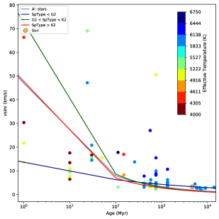
Figure 5: Projected rotational velocity, $v\sin i$, as a function of the stellar age. Different colours indicate the effective temperature of the stars. Solid lines indicate the best fit.

4.2 The stellar age - activity relationship

Figure 6 shows the stellar age as a function of the level of stellar activity in terms of $\log$R${}^{\rm{}^{\prime}}_{\rm HK}$. For an easy comparison with previous works we used the $\log$R${}^{\rm{}^{\prime}}_{\rm HK}$ values derived using the NO84 prescriptions. The dotted line shows the empirical relationship obtained by MH08.

It can be seen that the MH08 relationship predicts slightly younger ages for stars older than the Hyades. However, our sample is affected by several biases. To start with, only 23.3% of our stars have ages younger than $\sim$ 500 Myr (and only one has a colour index within the range of the NO84 calibrations). Another bias that might affect our results is the fact that at older ages our sample is mainly composed of stars with effective temperatures hotter than $\sim$ 5500 K and, therefore, they show lower levels of stellar activity than, otherwise similar, cooler stars. The dependency of the age-activity relationship on the spectral type, is quite clear when looking at the stars in the Hyades cluster, where it can be seen that cooler stars show higher levels of activity.

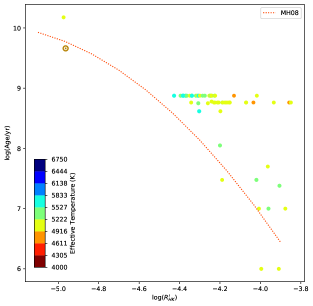
Figure 6: Stellar age as a function of $\log$R${}^{\rm{}^{\prime}}_{\rm HK}$. Different colours indicate the effective temperature of the stars. The dotted line shows the relationship obtained by MH08. The position of the Sun is shown with the symbol $\odot$.

4.3 Flux-flux relationships

Emission excesses in the Ca ii H & K and H$\alpha$ lines were determined by using the spectral subtraction technique (e.g. Montes et al., 1995, 2000). In brief, the basal chromospheric flux is removed by using the spectrum of a non-active star of similar stellar parameters and chemical composition to the target star as reference.

Reference stars were selected from Martínez-Arnáiz et al. (2010). Fluxes were derived from the measured equivalent width in the subtracted spectra by correcting the continuum flux

$$\log(F_{\lambda})=\log(EW)+\log(F^{\rm cont}_{\lambda})$$ (7)

where the continuum flux, $F^{\rm cont}_{\lambda}$, was determined by using the empirical calibrations with the colour index, $(B-V)$, derived by Hall (1996).

Figure 7 shows the comparison between the flux in the H$\alpha$ line and the flux in the Ca ii K line. A fit to a power-law function provides

$$\log(F_{H\alpha})=(4.58\pm 0.67)+(0.31\pm 0.11)\times\log(F_{CaK})$$ (8)

Martínez-Arnáiz et al. (2011a, b) identified two branches in the H$\alpha$ vs. Ca ii K flux-flux relationship. The lower or inactive branch has a slope of 1.17 $\pm$ 0.08 and is composed of field stars. On the other hand, the upper or active branch, is composed of young late-K and M stars and has a slope of 0.53 $\pm$ 0.08. Our sample provides a slope of 0.33 for the active branch showing that also young F-G stars share the behaviour of cooler young stars. However, we note that for most of our inactive stars we were not able to measure any emission excess, so we could identify only one star (namely HD 167389) in the inactive branch. Figure 7 also shows that there seems to be a tendency of higher H$\alpha$ fluxes for the youngest stars, that show a rather flat H$\alpha$ vs. Ca ii K relationship. We note that the different importance of H$\alpha$ and Ca ii emission might points to at a different role of different types of active structure (see Meunier & Delfosse, 2009, for the case of the Sun). It should also be noted that the formation of the H$\alpha$ line is much more subject to non-LTE effects than the Ca ii lines as well as to further complications in cool stars (this is because unlike the Ca ii H & K lines, the H$\alpha$ line is not a resonance transition). The star TYC 6779-305-1 shows a very strong emission in the H$\alpha$ line and departs from the other young stars in the flux-flux relationship.

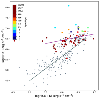
Figure 7: Flux-flux relationship between H$\alpha$ and Ca ii K. Different colours indicate the age of the stars. For comparison, data for FGKM stars from the literature (López-Santiago et al., 2010; Martínez-Arnáiz et al., 2010) are also plotted as grey circles. Our best linear fit for the upper branch is shown with a purple line, while the grey line shows the fit for the lower branch derived by Martínez-Arnáiz et al. (2011b).

5 Temporal evolution of active regions

5.1 Pooled variance analysis

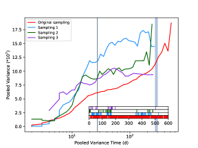
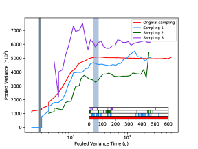
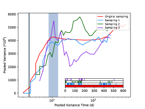
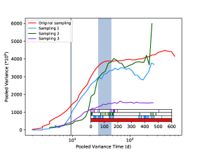
Figure 8: Pooled variance profile for the HARPS-N Solar S-index (up left), and simulated S-index time series, for different temporal samplings. The plot shows a smoothed function of the PV for ease reading of the plots. The vertical lines show the simulated rotation periods and AR lifetimes. The inset plots show the temporal coverage of the different samplings.

We apply the pooled variance (PV) technique (see e.g. Donahue et al., 1997a, b; Messina & Guinan, 2003; Lanza et al., 2004; Scandariato et al., 2017) to the time series of the Ca ii H & K activity index. In brief, the data are binned into time intervals of length $t_{\rm pool}$. Then, first the variance is calculated for each bin, and then the average of these variance values is computed forming the so-called pooled variance. This is done for a range of $t_{\rm pool}$ values across the duration of the monitoring observations. The characteristic timescales of the star are manifest as the position where the PV vs $t_{\rm pool}$ changes behaviour.

Before applying the PV method to our stars we performed a serie of simulations in order to understand the performance of the method as well as the effect of the sampling on the derivation of rotation periods and AR lifetimes. In our first test we took advantage of the solar spectra taken by the HARPS-N solar telescope and used the three years of S index values published in Maldonado et al. (2019). We computed the PV diagram using the original dataset and compared it with the PV diagram obtained by sampling the data using the observation times of three selected stars. The corresponding plot is shown in Figure 8 (top left). In detail, ’sampling 1’ contains 83 data points covering a time span of $\sim$ 1.5 yr. The data are divided into two main observing seasons with a gap of $\sim$ 200 d between them. ’Sampling 2’ is composed of 41 observation points taken in 1.3 yr. As in ’sampling 1’ there is a gap of 200 d between the two main observing seasons, but the second season is less populated than the first one. Finally, in ’Sampling 3’ we consider only 22 data points, covering $\sim$ 200 d, with a gap of $\sim$ 100 d between the two main observing seasons. The temporal coverage of the different samplings can be seen in the inset of the figure. The results show that even in the ’worst’ sampling (case 3, in purple) we are able to recover the rotation period with a value in the range 20 - 30 d. The AR lifetime is, however, only recovered when using the original time-serie (in red), with a value between 200 - 300 d.

Since the Sun is clearly not representative of most of our young stars, we performed three additional simulations. In simulation 1, (Fig. 8, top right) we consider a short rotation period of 2.74 d and an AR lifetime of 10 rotation periods. In simulation 2, (Fig. 8, bottom left) we keep the rotation period in 2.74 d but, consider an AR lifetime of 4 rotation periods. Finally, in simulation 3, (Fig. 8, bottom right) we fix the rotation period at 9.4 d, and the AR lifetime to 4 rotation periods. The simulations were performed by considering a sinusoidal behaviour, modulated with an exponential decay. In order to simulate the effect of spot growth and decay, as the time runs and the amplitude of the variability decays, another sinusoidal signal (with the same period but a different phase) is included.

It can be seen that in the short period cases, we are not able to recover the injected rotation period (even with the original dataset), as the PV steadily increases until the AR lifetime is reached. However, the AR lifetime seems well constrained even for samplings 1 and 2. In the case of sampling 3, without an a priory knowledge of the AR lifetime, we would have concluded that the PV diagram is too complex to derive any meaningful conclusion. Finally, for simulation 3, we are able to recover the AR lifetime in all cases. The injected rotation period is also recovered, although at a slightly shorter value, $\sim$ 7-8 d.

These simulations show that, with the data at hand, short rotation periods as well as long AR lifetimes may be difficult to identify by means of the PV technique. Therefore, we set a limit of at least 20 observations per star to use the method.

Figure 9 (up left) shows an example of a star (HD 59747) with a well-defined pattern. It can be seen that for this star the PV steadily increases up to a $t_{\rm pool}$ value of $\sim$ 8 d and then it shows a plateau where the PV remains roughly constant. The PV starts to increase again at $t_{\rm pool}$ $\sim$ 70 - 100 d. We conclude that the rotation period of this star is around 8 d, and that active regions have typical time scales for active region evolution of $\sim$ 10 rotation periods. We note that these estimates are in agreement with the results from the GLS and GP analysis.

Other stars like HD 45829 (Fig. 9, up right) show a different profile. In this case, the PV shows a small roughly constant value at small $t_{\rm pool}$ values. However, after $\sim$ 20 - 30 d, the PV shows a nearly-constant increase of variance with increasing time scale. These stars are dominated by non-periodic variations with substantial active region evolution masking the rotational plateau.

In stars like HD 235088 (Fig. 9, bottom left) the rotational plateau is not found and the PV increases until the active region evolution time scale is reached at $\sim$ 200 d. Other stars, show high PV at short time scale, but then, it diminishes. For example, HD 63433 (Fig. 9, bottom right) shows a peak at $\sim$ 7 d (in agreement with its rotation period) and then the PV steadily decreases (this can be due to statistical fluctuations due to a rather small number of data points in this interval of time or due to the presence of outliers) until it remains constant. Finally, some stars have rather complex patterns (e.g. TAP 26), the PV shows a large scatter, and their temporal variation is not well-defined, while stars like HIP 21112 show roughly constant patterns. Figure 16 shows the PV diagram for all stars with more than 20 observations.

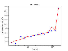
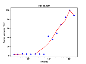
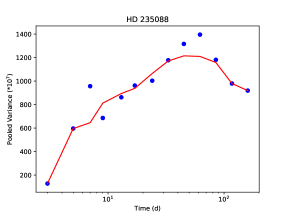
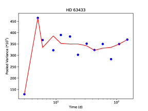
Figure 9: Pooled variance profile for HD 59747 (up left), HD 45289 (up right), HD 235088 (bottom left), and HD 63433 (bottom right). The red line is a smoothed function for easy reading of the plots that highlights the trend of the data.

5.2 AR lifetimes from light curve analysis

Once we have explored the behaviour of our sample in terms of the activity-age and flux-flux relationships, as well as in the pooled variance diagrams, we made use of available TESS photometry to study whether the inferred lifetimes of ARs show any dependency with the stellar properties, in particular, with the stellar age. Several recent works have made use of light curves to infer the properties of active regions. The idea behind these methods is that the decay-time of the autocorrelation function (ACF) is known to be related with the characteristic decay time of starspots (Lanza et al., 2014). In particular, Giles et al. (2017, hereafter GI17) modelled the ACF of light curves by using an underdamped harmonic oscillator with an interpulse term. However, Santos et al. (2021, hereafter SA21) discussed this choice of the modelling function, and suggested a new modelling with a linear decay. On the other hand, Basri et al. (2022, hereafter BA21) uses a method based on the strengths of the first few normalised autocorrelation peaks.

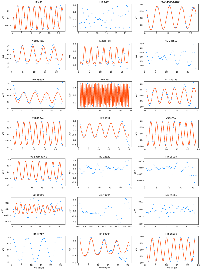
(a)

Figure 17: ACF curves of the TESS data. The red line shows the best fit.

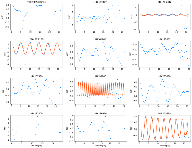
(b)

Figure 17: Continued.

In order to test whether these methods can be suitable for our stars, we start by computing the ACF of the TESS light curves. We note that the ACF can be calculated only for stars for which the data have a continuous sampling (or at least that can be interpolated to a continuous sampling). Otherwise, the strength of the ACF peaks might show a complicated dependency on the spectral window. The corresponding ACF curves are shown in Fig. 17, while the properties of the ACF analysis is given in Table 4.

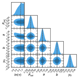
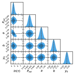
Figure 18: Posterior distribution of the ACF modelling for the star V830 Tau (left) and for the star HIP 105388 (right).

An inspection of the figure reveals that for some stars the peaks of the ACF have always the same strength (e.g. V830 Tau, TAP 26). That means that the active regions should be stable during the timespan of the observations. In addition, there seems to be no beating in these curves, usually due to differential rotation. Since the ACFs of these stars show no sign of time decay, it is unlikely that the methods presented in GI17, SA21, or BA21 might work. Indeed, if one try to fit the ACF curve of these stars to one of the functional forms described in GI17 or SA21, the result is that the posterior distribution of the AR lifetime is not well constrained, but shifted towards the larger prior of the AR lifetime. We illustrate this in the left panel of figure 18, where we show the posterior distribution for the case of the star V830 Tau. It is clear that while all parameters are well constrained, the fit is not able to derive any meaningful AR lifetimes. We classify these curves are ’sin’ (sinusoidal) or ’per’ (periodic) to indicate that there is no time-decay present in the ACF curve. With the data at hand, the only information that we can extract for these stars is that the typical AR lifetime should be much longer than the timespan of the observations.

Other stars like HIP 92680 and HIP 105388 show a clear time decay. For these stars, we used a bayesian framework to model the ACF curve to the functional forms described in GI17 (exponential decay) and SA21 (linear decay). As an example, we show the posterior distribution of the fit for the case of HIP 105388 (Fig. 18, right). We used the Bayesian Inference Criterion (BIC) as a measure of the goodness of the two models, although in most cases the BIC of the two models are almost identical (that is, there is no significant evidence in supporting one model against the other). We note that for some stars, even if the posterior distribution of all the fitted parameters are well constrained, the best fit is not able to reproduce all the features seen in the ACF (e.g. V1090 Tau or V1298 Tau). This might indicate that these ACFs are not fully regular. Indeed, some of our stars show a rather irregular ACF curve that makes difficult its analysis. Some examples are HD 285507, or HD 32923. Table 4 provides the AR lifetimes or lower limits derived, when possible, from the ACF curves.

Table 4: Summary of the ACF analysis of the TESS light curves.

Star	ACF-fit $\tau$ (d)	ACF-type	ACF-fit form
HIP 490	232.59${}_{\rm-106.83}^{\rm+474.93}$	sin + decay	exp
HIP 1481		sin + decay	bad fit
TYC 4500-1478-1	132.92${}_{\rm-52.46}^{\rm+248.64}$	sin + decay	exp
V1090 Tau	135.47${}_{\rm-66.71}^{\rm+407.07}$	sin + decay	exp†
V1298 Tau	259.36${}_{\rm-155.05}^{\rm+687.93}$	per + decay	lin†
HD 285507		other
HIP 19859	$>>$ 26	per
TAP 26	$>>$ 24	per
HD 285773	$>>$ 25	per
V1202 Tau	$>>$ 24	sin
HIP 21112	$>>$ 26	sin
V830 Tau	$>>$ 24	sin
TYC 5909-319-1	387.19${}_{\rm-238.44}^{\rm+761.66}$	sin + decay?	exp†
HD 32923		other
HD 36108		other
HD 38283	42.19${}_{\rm-15.72}^{\rm+89.43}$	per	exp†
HIP 27072		other
HD 45289		other
HD 59747	$>>$ 27	sin
HD 63433	62.31${}_{\rm-14.29}^{\rm+37.82}$	sin + decay	lin†
HD 70573	$>>$ 25	sin
TYC 1989-0049-1		other
HD 107877		other
BD+26 2342	64.07${}_{\rm-18.58}^{\rm+55.15}$	sin + decay?	exp
BD+27 2139	$>>$ 27	sin
HIP 61205		other
HD 122862		other
HD 167389		other	bad fit
HIP 92680	232.93${}_{\rm-155.27}^{\rm+714.18}$	per + decay	lin
HD 235088		other
HD 191408		other
HD 196378		other
HIP 105388	82.95${}_{\rm-18.16}^{\rm+33.26}$	per + decay	exp

5.3 AR lifetime as a function of the stellar parameters

Figure 10, top left, shows the timescale of AR evolution derived from the ACF analysis of the TESS light curves as a function of the stellar age. Given that the number of points is rather low and also the uncertainties involved in age and AR lifetime, any conclusion from this figure should be taken with caution. Nevertheless, the figure reveals a tendency of younger stars to show longer AR lifetimes. The Spearman’s rank test, $\rho$, is -0.67 with a p-value of 0.03 (the lower limits on AR lifetimes were not considered).

We also checked for correlations between AR lifetimes, the effective temperature of the star (Fig. 10, top right), and the level of activity (as measured by the $\log$R${}^{{}^{\prime}}_{\rm HK}$ value), Fig. 10, bottom left. A general tendency of increasing AR lifetime with cooler temperatures and higher activity levels seems to be present in the data. Whilst the AR lifetime correlation with T_eff might be statistically significant (with a p-value lower than 0.02), the one with the level of activity does not (p-value $\sim$ 0.12). These results are in agreement with GI17, SA21 or BA22 who analysing a large dataset of Kepler light curves concluded that ARs decay more slowly in cooler stars.

It is worth noticing that when comparing stars with different stellar parameters, other properties like the convective turnover time might be different as well. The use of the Rossby number has been shown to improve substantially the observed activity-rotation relations for main sequence, solar-type stars (e.g. Noyes et al., 1984). To compute the Rossby number, we first estimate the mass of our stars by using the Gaia DR2 luminosities (Gaia Collaboration, 2018) and the mass-luminosity relationship provided by Wang & Zhong (2018). We then derive the convective turnover timescales by interpolating (in stellar mass and age) the theoretical tracks provided by Spada et al. (2013). Figure 11 shows the position of our target stars in the stellar mass-age diagram where it can be seen that most of our targets have masses in the 0.8 - 1.1 M_⊙ range. Finally, the Rossby number is computed as

$$R_{\rm 0}=\frac{P_{\rm rot}}{\tau_{\rm conv}}$$ (9)

Figure 10, bottom right, shows the timescale of AR evolution as a function of the Rossby number. For a better comparison between stars with different properties we show the AR lifetime in units of the corresponding rotational period. The figure shows a clear tendency of decreasing AR lifetimes with increasing Rossby number, which would imply that ARs survive longer in stars with larger convective turnover timescales and shorter rotation period. A Spearman’s correlation test returns the values $\rho$ = -0.64 and $p$-value = 0.05.

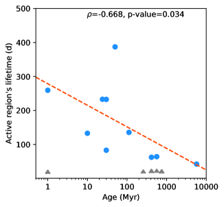
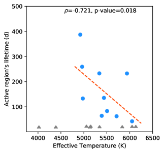
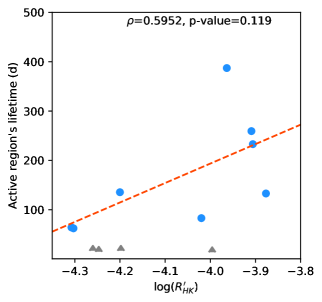
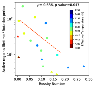
Figure 10: Timescale of AR evolution derived from the ACF analysis of the TESS light curves as a function of the stellar age (top left), the effective temperature (top right), the $\log$R${}^{{}^{\prime}}_{\rm HK}$ value (bottom left), and the Rossby number (bottom right). Stars with lower limits on AR timescale are shown with triangles. A linear fit is (dashed orange-red line) is shown for for guiding the eye.

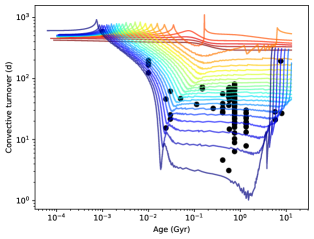
Figure 11: Convective turnover timescale as a function of the stellar age. The black circles show the stars studied in this work while the continuous lines represents the tracks provided by Spada et al. (2013). The models have solar metallicities and stellar masses ranging from 0.10 M _⊙ to 1.25 M_⊙ (from red to violet) with a mass step of 0.05 M_⊙.

5.4 Gaussian process analysis of the spectroscopic indexes

In this section we explore whether our spectroscopic time series can be used to infer the AR lifetimes. That would be of the utmost interest as it will provide a complementary approach to the use of light curve ACFs. Through this analysis we use the results of the GP analysis (see Sect. 3.4) and make the assumption that the GP hyperparameter $\tau$ (that is, the timescale of the exponential decay, see Eqn. 5) corresponds to the AR growth and decay lifetime. Whether this assumption is well founded or not will be discussed below.

For this analysis we focus only on stars with more than twenty observations and with available TESS photometry. Since most of our targets are young, they should have short rotation periods and therefore, the rotation periods derived from the TESS data should be reliable. We note that the use of GP analysis to derive rotation period has already been used in the literature (e.g. Angus et al., 2018). However, given that the rotation period is a key parameter of the analysis, we performed a comparison with other photometric surveys like ASAS (Shappee et al., 2014; Jayasinghe et al., 2019), SWAPS (Butters, O. W. et al., 2010), STELLA (Strassmeier et al., 2004), as well as other literature sources. Table 5 provides a summary of the derived rotation periods. The TESS rotation periods are derived from our GP analysis.

In addition, the TESS-derived periods can be translated into equatorial velocities, v_eq, and compared with the corresponding v$\sin i$ values. In order to perform this conversion, stellar radii are taken from Gaia DR2 (Gaia Collaboration, 2018). The corresponding plot is shown in Fig. 12. As expected, most of the targets lie in the region v_eq larger than v$\sin i$, while 14 stars are close to the line v_eq $\sim$ v$\sin i$ and should have inclination angles $\sim$ 90 degrees. We note that one star, namely HD 107877, have P_rot a value that translates into non-physical v_eq values (i.e., shorter than v$\sin i$). For this star no clear P_rot was found in the analysis of the ASAS or SWAPS photometry, while the STELLA data show two peaks at $\sim$ 7.3 d and $\sim$ 1.6 d. We note that the 7.3 d signal is still too large, to be compatible with the v$\sin i$ value.

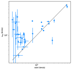
Figure 12: Equatorial velocities (derived from the TESS P_rot and R_⋆) versus projected rotational velocities, v$\sin i$.

Table 5: Rotational periods derived from TESS, ASAS, SWAPS, PV analysis and the literature.

Star	TESS	ASAS	SWAPS	Other	Pooled Variance
	(d)	(d)	(d)	(d)	(d)
HIP 490	3.01
HIP 1481	2.41				$\sim$ 3
TYC 4500-1478-1†	3.39	3.42		3.5 (STELLA)	$\sim$ 6
V1090 Tau†	4.68	4.76	4.71
V1298 Tau†	2.91		2.89/1.44	2.91 (Suárez Mascareño et al., 2021)
HD 285507	5.76	10.57		2.24 (Carleo et al., 2020)
HIP 19859	5.85
TAP 26†	0.71	0.71		0.71 (Grankin, 2013)
HD 285773	5.14	1.9/4.6		10.7? (Douglas et al., 2019)	$\sim$ 6
V1202 Tau†	2.72	2.7	1.59	2.68 (STELLA)
HIP 21112	5.40
V830 Tau†	2.77	2.74	1.37	2.74 (Damasso et al., 2020)
TYC 5909-319-1†	3.42	3.37	1.41/3.4	3.43 (Carleo et al., 2021)
HD 32923	3.43			32 (Schmitt & Mittag, 2020)	$\sim$ 3/4
HD 36108	2.48		2.99?		$\sim$ 2/3
HD 38283	2.36
HIP 27072†	6.21			5.9 (Montesinos et al., 2016)
HD 45289	4.37
HD 59747†	8.04				$\sim$ 8
HD 63433†	6.48		7.98	6.45 (Mann et al., 2020)	$\sim$ 4/5?
HD 70573†	3.32			3.28 (STELLA)
TYC 1989-0049-1	12.16	8.27	10.86	5.5/11 (STELLA)
HD 107877	9.25			7.3?/1.16? (STELLA)
BD+26 2342†	4.99			4.6 (GAPS data)
BD+27 2139†	9.37		9.29	9.28 (STELLA)	$\sim$ 4/5?
HIP 61205	5.91		7.58	7.39 (STELLA)
HD 122862	3.80				$\sim$ 3
HD 167389†	7.70			8.85 (GAPS data)	$\sim$ 7/8
HIP 92680	1.00
HD 235088	6.14			14.1 (REM), 12.8-13.5 (STELLA)
HD 191408	3.44
HD 196378	8.86
HIP 105388	3.39

In the following we will retain for study only those star for which the number of spectroscopic observations is larger than twenty, they have TESS photometry, and we have at least one independent confirmation that the TESS-derived period is correct. These stars are highlighted in Table 5.

Figure 13 shows the rotation periods derived from the GP analysis of the Ca ii, the Balmer lines, He i D₃, and Na i D₁, D₂ activity indexes as a function of the reference TESS-derived rotatin periods. The corresponding comparison for the derived AR lifetimes is shown in Fig. 14.

We note that for most of the stars the rotation periods derived from the spectroscopic indexes are significantly shorter than the TESS-derived periods. For example, for BD+27 2139 (which has a TESS-derived period of 9.37 d) the analysis of the different spectroscopic indexes provide values in the range $\sim$ 2 -3 d. On the other hand, AR lifetimes derived from spectroscopic indexes are much longer than those derived from the TESS data.

Furthermore, even if the periods from different indexes agree, AR lifetimes can be very different from one index to another. An example is the star V830 Tau, for which we recover a rotation period of $\sim$ 2.77 d in TESS, Ca ii, H$\delta$, and H$\epsilon$ data. However, the AR lifetime varies from $\sim$ 5.32 d in the TESS data to $\sim$ 2970 d in the Ca ii H & K data (we note that for this star, from the ACF light curve analysis we only concluded that its AR lifetime should be longer than 24 d.)

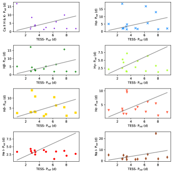
Figure 13: Derived rotation periods from the GP analysis of the different spectroscopic indexes as a function of the values derived from the GP analysis of the TESS photometry.

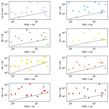
Figure 14: Derived AR lifetimes from the GP analysis of the different spectroscopic indexes as a function of the values derived from the GP analysis of the TESS photometry.

We conclude that the GP analysis of the spectroscopic indexes does not allow us to measure AR lifetimes to a useful accuracy. Several explanations can be put forward to account for this result. The first one deals with the data and the assumptions used in this work. We note that the bulk of the stars analysed in this work comes from a radial velocity exoplanet program, and therefore, the number of observations, temporal baseline, and sampling vary considerably from one star to another and in some cases it may not be optimal. Although stating the obvious, we recall that only stars in which potential planetary signals are identified are observed with a high cadence. Furthermore, it is important to keep in mind that GPs are simplified ad hoc models of stellar activity and that the correspondence between the GP hyperparameters and the physical properties of AR should be further analysed.

6 Conclusions

In this work a detailed analysis of a large sample of young stars with well known derived ages determined from their membership to kinematic associations and moving groups is performed. Projected rotational velocities and activity indexes are determined in an homogeneous way from high-resolution optical spectra. The temporal series of the different activity indexes are used together with a gaussian process regression analysis to infer rotational periods and the lifetime of AR growth and decay.

We characterise our sample in terms of activity-rotation-age and flux-flux relationships and confirm the well known trend of decreasing activity and rotation with stellar age. We also show that cooler stars show higher levels of activity, and that their rotation rate shows a lower age-decay than their hotter counterparts. We also find that young F, G stars depart from the inactive stars in the flux-flux relationships.

We search for correlations between the ARs evolution lifetime and the stellar properties, namely age, effective temperature, and level of activity. AR lifetimes derived from the ACF analysis of light curves show a tendency to decrease with the stellar age. ARs lifetimes are also found to be lower in hotter and inactive stars. A global tendency of larger ARs lifetimes versus lower Rossby number is also found. However, we caution that these relationships are affected by the low number of stars for which a reliable AR lifetime could be obtained. Finally, one cannot forget the assumptions linked to the models used to determine stellar ages or the convective turnover timescale. We also tried to derive AR lifetimes from a GP modelling of the spectroscopic time-series, but the results were largely unsatisfactory, even if we restricted the analysis to stars with well known rotation periods from photometric data.

Further observations of stars covering a wide range of stellar ages, together with a better understanding of how to model stellar activity, as well as an accurate determination of the stellar properties will help us to understand whether ARs have rather irregular lifetimes or if there is some unknown relationship between ARs lifetimes and stellar properties.

Appendix A The (B-V) colour - T_eff relationship

In order to derive a relationship between the effective temperature and the (B-V) colour we use the data from Flower (1996, Table 3). The data was fitted to a seven order polynomial fit of the form: $(B-V)$ = a₀ + a₁$\times$$(\log T_{\rm eff})$ + a₂$\times$$(\log T_{\rm eff})^{2}$ + … + a₇$\times$$(\log T_{\rm eff})^{7}$. Table 6 gives the coefficients of the polynomial fit.

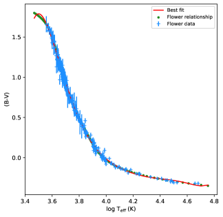
Figure 15: (B-V) vs. $\log$T_eff relationship. The blue crosses show the data for the individual main-sequence stars while the green dots corresponds to the colour-T_eff scale presented in Flower (1996). Our best fit is shown in red.

Table 6: Coefficients of the (B-V) vs. $\log$T_eff relationship.

Coefficient	Value
a0	-6.5459$\times$105
a1	1.0991$\times$106
a2	-7.8965$\times$105
a3	3.1471$\times$105
a4	-7.5147$\times$104
a5	1.0752$\times$104
a6	-8.5347$\times$102
a7	2.8998$\times$101

Appendix B Online Figures

Figure 16 shows the pooled variance profile for all the stars with more than 20 observations.

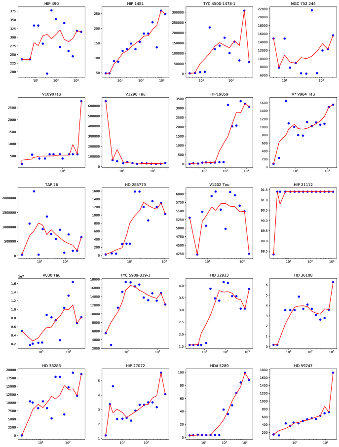
(a)

Figure 16: Pooled variance profile for stars with more than 20 observations. The red line is a smoothed function for ease reading of the plots.

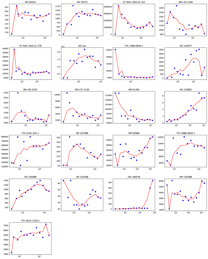
(b)

Figure 16: Continued.

Appendix C Online Tables

Table LABEL:longtable_kinematicis provides the kinematic data of the stars analysed in this work. Namely, star identifier (column 1), galactic-spatial velocity components (columns 2, 3, and 4), preliminary young stellar group or association (column 5), best hypothesis and probability (columns 6 and 7) for stellar group or association membership obtained using the BANYAN tool (Gagné et al. 2018).

1]

Table 7: Galactic-spatial velocity components and membership to stellar kinematic groups and associations.

Star	$U$	$V$	$W$	Association	Best hypothesis	Probability
	(kms-1)	(kms-1)	(kms-1)
HIP 490	-9.30 $\pm$ 0.06	-20.92 $\pm$ 0.04	-1.91 $\pm$ 0.23	TUC	TUC	0.9998
HIP 1481	-9.51 $\pm$ 0.12	-20.69 $\pm$ 0.15	-0.38 $\pm$ 0.26	TUC	TUC	0.9999
TYC 4500-1478-1	-6.65 $\pm$ 0.68	-13.37 $\pm$ 1.07	-4.67 $\pm$ 0.37	Cepheus	Field	0.0000
HD 3823	-111.57 $\pm$ 0.13	-17.94 $\pm$ 0.06	-35.52 $\pm$ 0.12	Field	Field	0.0000
HIP 8486	19.56 $\pm$ 0.14	4.66 $\pm$ 0.05	-2.45 $\pm$ 0.21	Ursa Major	Field	0.0000
NGC 752 48	-17.26 $\pm$ 0.89	-19.90 $\pm$ 1.15	-21.24 $\pm$ 0.83	NGC 752	Field	0.0000
Cl* NGC 752 RV 144	-15.88 $\pm$ 0.22	-21.12 $\pm$ 0.27	-18.57 $\pm$ 0.20	NGC 752	Field	0.0000
NGC 752 80	-18.77 $\pm$ 1.63	-17.20 $\pm$ 1.53	-20.35 $\pm$ 0.98	NGC 752	Field	0.0000
NGC 752 151	-15.91 $\pm$ 0.36	-20.90 $\pm$ 0.36	-18.43 $\pm$ 0.23	NGC 752	Field	0.0000
NGC 752 185	-20.37 $\pm$ 1.87	-20.52 $\pm$ 1.78	-19.87 $\pm$ 1.12	NGC 752	Field	0.0000
NGC 752 184	-14.87 $\pm$ 0.41	-22.75 $\pm$ 0.41	-17.34 $\pm$ 0.26	NGC 752	Field	0.0000
NGC 752 211	-17.42 $\pm$ 0.87	-19.51 $\pm$ 0.82	-18.48 $\pm$ 0.51	NGC 752	Field	0.0000
NGC 752 229	-20.27 $\pm$ 2.37	-15.65 $\pm$ 2.19	-22.02 $\pm$ 1.41	NGC 752	Field	0.0000
NGC 752 229	-20.27 $\pm$ 2.37	-15.65 $\pm$ 2.19	-22.02 $\pm$ 1.41	NGC 752	Field	0.0000
NGC 752 236	-19.04 $\pm$ 2.71	-18.29 $\pm$ 2.50	-20.33 $\pm$ 1.61	NGC 752	Field	0.0000
NGC 752 244	-13.53 $\pm$ 0.24	-22.11 $\pm$ 0.27	-18.65 $\pm$ 0.19	NGC 752	Field	0.0000
NGC 752 268	-16.96 $\pm$ 2.14	-19.10 $\pm$ 1.99	-18.92 $\pm$ 1.24	NGC 752	Field	0.0000
HIP 14976	-40.85 $\pm$ 0.20	-19.41 $\pm$ 0.10	-0.88 $\pm$ 0.09	HYA	HYA	0.8410
HIP 15310	-43.47 $\pm$ 0.12	-23.43 $\pm$ 0.03	-1.47 $\pm$ 0.10	HYA	Field	0.0000
HD 20794	-78.71 $\pm$ 0.08	-93.03 $\pm$ 0.23	-29.41 $\pm$ 0.36	Field	Field	0.0000
HIP 16529	-41.71 $\pm$ 0.11	-19.17 $\pm$ 0.04	-0.69 $\pm$ 0.06	HYA	HYA	0.9956
HD 22879	-111.00 $\pm$ 0.15	-90.86 $\pm$ 0.10	-43.08 $\pm$ 0.15	Field	Field	0.0000
TYC 1804-1924-1	-7.97 $\pm$ 0.66	-27.31 $\pm$ 0.21	-15.60 $\pm$ 0.29	PLE	PLE	0.9994
V1090 Tau	-7.95 $\pm$ 0.29	-27.88 $\pm$ 0.10	-13.88 $\pm$ 0.13	PLE	PLE	0.9998
V* V471 Tau	-43.68 $\pm$ 0.44	-18.26 $\pm$ 0.06	-2.67 $\pm$ 0.23	HYA	HYA	0.9739
HD 283066	-41.82 $\pm$ 0.35	-19.23 $\pm$ 0.08	-1.12 $\pm$ 0.15	HYA	HYA	0.9990
HD 283044	-43.23 $\pm$ 0.33	-19.31 $\pm$ 0.08	-1.71 $\pm$ 0.14	HYA	HYA	0.9972
HD 286363	-42.21 $\pm$ 0.17	-18.87 $\pm$ 0.02	-1.43 $\pm$ 0.10	HYA	HYA	0.9911
HIP 18327	-42.59 $\pm$ 0.16	-18.55 $\pm$ 0.03	-1.40 $\pm$ 0.08	HYA	HYA	0.9995
HD 285348	-41.31 $\pm$ 0.33	-19.70 $\pm$ 0.05	-1.07 $\pm$ 0.15	HYA	HYA	0.9975
V1298 Tau	-12.68 $\pm$ 0.01	-6.35 $\pm$ 0.02	-9.07 $\pm$ 0.02	Taurus	Taurus	0.9976
HG 7-88	-42.85 $\pm$ 0.24	-19.26 $\pm$ 0.04	-1.57 $\pm$ 0.11	HYA	HYA	0.9991
HIP 19098	-42.02 $\pm$ 0.19	-19.35 $\pm$ 0.03	-0.50 $\pm$ 0.09	HYA	HYA	0.9993
HIP 19148	-42.31 $\pm$ 0.13	-18.62 $\pm$ 0.02	-1.43 $\pm$ 0.07	HYA	HYA	0.9982
HD 285507	-42.74 $\pm$ 0.38	-18.66 $\pm$ 0.03	-1.60 $\pm$ 0.19	HYA	HYA	0.9992
HIP 19781	-42.01 $\pm$ 0.16	-17.93 $\pm$ 0.02	-0.92 $\pm$ 0.08	HYA	HYA	0.9908
HIP 19786	-42.06 $\pm$ 0.20	-19.34 $\pm$ 0.03	-1.17 $\pm$ 0.10	HYA	HYA	0.9983
HIP 19793	-42.46 $\pm$ 0.14	-19.34 $\pm$ 0.03	-1.37 $\pm$ 0.05	HYA	HYA	0.9992
HIP 19796	-42.40 $\pm$ 0.27	-18.74 $\pm$ 0.02	-1.15 $\pm$ 0.14	HYA	HYA	0.9984
HIP 19859	14.44 $\pm$ 0.13	-0.50 $\pm$ 0.02	-10.04 $\pm$ 0.08	Ursa Major	Field	0.0000
HD 285590	-42.46 $\pm$ 0.58	-19.42 $\pm$ 0.03	-0.98 $\pm$ 0.27	HYA	HYA	0.9996
V* V984 Tau	-42.54 $\pm$ 0.16	-19.06 $\pm$ 0.03	-1.51 $\pm$ 0.06	HYA	HYA	0.9984
TAP 26	-18.18 $\pm$ 5.27	-6.10 $\pm$ 0.23	-11.53 $\pm$ 2.22	Taurus	Taurus	0.9965
HIP 20130	-42.40 $\pm$ 0.24	-19.22 $\pm$ 0.03	-1.41 $\pm$ 0.09	HYA	HYA	0.9996
HIP 20146	-41.63 $\pm$ 0.27	-19.13 $\pm$ 0.03	-0.75 $\pm$ 0.11	HYA	HYA	0.9996
HIP 20237	-42.07 $\pm$ 0.15	-19.13 $\pm$ 0.04	-1.27 $\pm$ 0.06	HYA	HYA	0.9997
HIP 20480	-42.21 $\pm$ 0.23	-18.68 $\pm$ 0.03	-1.66 $\pm$ 0.08	HYA	HYA	0.9989
V* V988 Tau	-42.42 $\pm$ 1.86	-17.54 $\pm$ 0.58	-3.91 $\pm$ 0.77	HYA	HYA	0.9739
HD 27771	-42.36 $\pm$ 0.24	-18.65 $\pm$ 0.02	-0.96 $\pm$ 0.11	HYA	HYA	0.9995
HIP 20557	-42.03 $\pm$ 0.15	-19.09 $\pm$ 0.03	-1.22 $\pm$ 0.05	HYA	HYA	0.9996
V* V990 Tau	-42.72 $\pm$ 0.17	-19.32 $\pm$ 0.02	-1.05 $\pm$ 0.07	HYA	HYA	0.9997
HD 285742	-42.01 $\pm$ 0.82	-19.06 $\pm$ 0.03	-1.63 $\pm$ 0.33	HYA	HYA	0.9942
HIP 20741	-40.99 $\pm$ 0.14	-19.56 $\pm$ 0.03	-1.56 $\pm$ 0.06	HYA	HYA	0.9991
HD 286820	-43.87 $\pm$ 0.70	-15.43 $\pm$ 0.28	-5.16 $\pm$ 0.43	HYA	Field	0.0046
HIP 20815	-41.96 $\pm$ 0.15	-19.14 $\pm$ 0.02	-1.22 $\pm$ 0.06	HYA	HYA	0.9997
HIP 20826	-41.48 $\pm$ 0.16	-19.19 $\pm$ 0.02	-0.85 $\pm$ 0.08	HYA	HYA	0.9994
HIP 20850	-43.63 $\pm$ 0.65	-18.17 $\pm$ 0.08	-1.96 $\pm$ 0.29	HYA	HYA	0.9990
HD 28258	-43.63 $\pm$ 0.65	-18.17 $\pm$ 0.08	-1.96 $\pm$ 0.29	HYA	HYA	0.9990
HIP 20899	-41.94 $\pm$ 0.14	-19.37 $\pm$ 0.02	-0.45 $\pm$ 0.06	HYA	HYA	0.9996
HIP 20951	-42.10 $\pm$ 0.10	-19.30 $\pm$ 0.02	-1.28 $\pm$ 0.04	HYA	HYA	0.9997
HD 285773	-42.10 $\pm$ 0.10	-19.30 $\pm$ 0.02	-1.28 $\pm$ 0.04	HYA	HYA	0.9997
HIP 20978	-42.57 $\pm$ 0.21	-19.17 $\pm$ 0.02	-1.38 $\pm$ 0.08	HYA	HYA	0.9998
HD 28462	-42.57 $\pm$ 0.21	-19.17 $\pm$ 0.02	-1.38 $\pm$ 0.08	HYA	HYA	0.9998
HIP 21099	-42.63 $\pm$ 0.14	-19.42 $\pm$ 0.02	-1.07 $\pm$ 0.05	HYA	HYA	0.9996
V1202 Tau	-12.54 $\pm$ 0.02	-6.09 $\pm$ 0.02	-9.59 $\pm$ 0.02	Taurus	Taurus	0.9991
HIP 21112	-42.01 $\pm$ 0.21	-15.36 $\pm$ 0.12	-1.43 $\pm$ 0.15	HYA	Field	0.0116
V830 Tau	-12.85 $\pm$ 2.48	-11.56 $\pm$ 0.26	-8.56 $\pm$ 0.70	Taurus	Taurus	0.9981
HIP 21317	-42.01 $\pm$ 0.13	-19.39 $\pm$ 0.02	-1.61 $\pm$ 0.05	HYA	HYA	0.9996
HIP 21654	-43.59 $\pm$ 0.21	-21.08 $\pm$ 0.33	-0.49 $\pm$ 0.28	HYA	HYA	0.9939
HIP 22203	-42.81 $\pm$ 0.28	-19.35 $\pm$ 0.08	-1.51 $\pm$ 0.11	HYA	HYA	0.9995
HD 284787	-44.69 $\pm$ 1.71	-20.07 $\pm$ 0.21	-3.08 $\pm$ 0.47	HYA	HYA	0.9607
HIP 22422	-42.13 $\pm$ 0.13	-19.19 $\pm$ 0.02	-0.80 $\pm$ 0.05	HYA	HYA	0.9995
HIP 23069	-42.24 $\pm$ 0.27	-18.92 $\pm$ 0.04	-1.20 $\pm$ 0.09	HYA	HYA	0.9983
HIP 23498	-41.78 $\pm$ 0.32	-18.88 $\pm$ 0.05	-1.15 $\pm$ 0.10	HYA	HYA	0.9977
HIP 23750	-42.15 $\pm$ 0.26	-19.13 $\pm$ 0.03	-1.38 $\pm$ 0.06	HYA	HYA	0.9969
TYC 5909-319-1	-14.70 $\pm$ 0.71	-21.34 $\pm$ 0.61	-4.45 $\pm$ 0.58	Field	Field	0.0000
HD 32923	-26.10 $\pm$ 0.15	-23.64 $\pm$ 0.10	28.35 $\pm$ 0.14	Field	Field	0.0000
HIP 25486	-11.59 $\pm$ 0.38	-15.93 $\pm$ 0.26	-8.99 $\pm$ 0.21	Beta Pic	Beta Pic	0.9993
HD 36108	-35.23 $\pm$ 0.09	7.03 $\pm$ 0.10	-24.36 $\pm$ 0.07	Field	Field	0.0000
HD 38283	31.70 $\pm$ 0.04	-60.94 $\pm$ 0.15	-7.82 $\pm$ 0.09	Field	Field	0.0000
HIP 27072	17.95 $\pm$ 0.02	4.25 $\pm$ 0.00	-11.75 $\pm$ 0.02	Ursa Major	Field	0.0000
HD 45289	-115.09 $\pm$ 0.06	-22.82 $\pm$ 0.13	-3.76 $\pm$ 0.06	Field	Field	0.0000
HD 59747	12.65 $\pm$ 0.15	2.76 $\pm$ 0.01	-10.42 $\pm$ 0.06	Ursa Major	Field	0.0000
HD 63433	14.10 $\pm$ 0.18	2.54 $\pm$ 0.04	-7.97 $\pm$ 0.08	Ursa Major	Field	0.0000
HD 70573	-15.80 $\pm$ 0.19	-21.30 $\pm$ 0.18	-10.53 $\pm$ 0.10	Hercules-Lyra	Field	0.0000
Cl* NGC 2632 JC 61	-43.54 $\pm$ 1.18	-20.31 $\pm$ 0.58	-8.25 $\pm$ 0.81	PRAE	PRAE	0.9998
Cl* NGC 2632 JS 133	-42.17 $\pm$ 0.67	-19.78 $\pm$ 0.31	-10.15 $\pm$ 0.47	PRAE	PRAE	0.9999
Cl* NGC 2632 JS 142	-41.98 $\pm$ 1.71	-19.88 $\pm$ 0.78	-9.71 $\pm$ 1.18	PRAE	PRAE	0.9998
Cl* NGC 2632 JS 143	-42.62 $\pm$ 0.99	-20.19 $\pm$ 0.46	-9.54 $\pm$ 0.69	PRAE	PRAE	0.9999
Cl* NGC 2632 JS 247	-43.76 $\pm$ 1.15	-20.77 $\pm$ 0.53	-9.02 $\pm$ 0.81	PRAE	PRAE	0.9999
Cl* NGC 2632 JC 141	-43.40 $\pm$ 0.81	-20.37 $\pm$ 0.40	-9.32 $\pm$ 0.57	PRAE	PRAE	0.9999
Cl* NGC 2632 JC 158	-42.91 $\pm$ 1.00	-20.52 $\pm$ 0.48	-9.04 $\pm$ 0.71	PRAE	PRAE	1.0000
Cl* NGC 2632 JC 172	-44.45 $\pm$ 1.78	-21.35 $\pm$ 0.86	-8.31 $\pm$ 1.26	PRAE	PRAE	0.9999
Cl* NGC 2632 JC 208	-43.24 $\pm$ 1.30	-19.34 $\pm$ 0.64	-9.41 $\pm$ 0.93	PRAE	PRAE	0.9999
Cl* NGC 2632 JC 221	-42.10 $\pm$ 1.20	-20.44 $\pm$ 0.61	-8.49 $\pm$ 0.85	PRAE	PRAE	0.9998
Cl* NGC 2632 JS 404	-43.44 $\pm$ 0.66	-21.18 $\pm$ 0.31	-9.97 $\pm$ 0.48	PRAE	PRAE	0.9999
Cl* NGC 2632 JC 234	-44.04 $\pm$ 0.60	-19.86 $\pm$ 0.30	-9.84 $\pm$ 0.44	PRAE	PRAE	0.9998
K2 101	-42.89 $\pm$ 0.67	-20.44 $\pm$ 0.34	-10.01 $\pm$ 0.49	PRAE	PRAE	1.0000
BD+20 2184	-41.81 $\pm$ 0.37	-20.45 $\pm$ 0.18	-9.36 $\pm$ 0.29	PRAE	PRAE	0.9999
Cl* NGC 2632 WJJP 792	-42.52 $\pm$ 0.81	-21.88 $\pm$ 0.39	-9.72 $\pm$ 0.59	PRAE	PRAE	0.9997
Cl* NGC 2632 JC 278	-42.67 $\pm$ 0.36	-20.07 $\pm$ 0.18	-9.92 $\pm$ 0.27	PRAE	PRAE	1.0000
Cl* NGC 2632 KW 551	-42.01 $\pm$ 0.64	-20.70 $\pm$ 0.33	-9.77 $\pm$ 0.47	PRAE	PRAE	0.9999
Cl* NGC 2632 JS 563	-41.78 $\pm$ 0.53	-19.78 $\pm$ 0.28	-9.31 $\pm$ 0.40	PRAE	PRAE	0.9999
Cl* NGC 2632 JS 576	-42.15 $\pm$ 1.23	-20.22 $\pm$ 0.59	-9.27 $\pm$ 0.91	PRAE	PRAE	0.9999
AD Leo	-15.00 $\pm$ 0.00	-7.49 $\pm$ 0.00	3.52 $\pm$ 0.00	Castor MG	Field	0.0000
TYC 1989-0049-1	-2.16 $\pm$ 0.04	-5.54 $\pm$ 0.03	-0.90 $\pm$ 0.37	CBER	CBER	1.0000
HD 107877	-2.71 $\pm$ 0.03	-5.26 $\pm$ 0.03	-0.29 $\pm$ 0.35	CBER	CBER	0.9999
BD+26 2342	-2.45 $\pm$ 0.05	-5.66 $\pm$ 0.04	-0.64 $\pm$ 0.61	CBER	CBER	1.0000
BD+27 2139	-2.67 $\pm$ 0.02	-5.79 $\pm$ 0.02	0.80 $\pm$ 0.21	CBER	CBER	0.9999
HIP 61205	-1.95 $\pm$ 0.04	-5.94 $\pm$ 0.03	-0.68 $\pm$ 0.32	CBER	Field	0.3090
BD+23 2472	-1.93 $\pm$ 0.02	-4.40 $\pm$ 0.05	-2.33 $\pm$ 0.39	CBER	CBER	0.9027
HD 122862	-27.57 $\pm$ 0.10	-4.91 $\pm$ 0.12	37.76 $\pm$ 0.04	Field	Field	0.0000
TYC 6779-305-1	-3.97 $\pm$ 0.62	-17.35 $\pm$ 0.13	-6.68 $\pm$ 0.26	Upper Sco	Upper Sco	0.9959
TYC 6191-552-1	-7.00 $\pm$ 0.62	-15.45 $\pm$ 0.09	-6.29 $\pm$ 0.30	Upper Sco	Upper Sco	0.9983
GSC 06204-00812	-4.27 $\pm$ 1.15	-15.25 $\pm$ 0.13	-7.37 $\pm$ 0.55	Upper Sco	Upper Sco	0.9987
V866 Sco				Upper Sco	Upper Sco	0.9711
HD 167389	17.20 $\pm$ 0.05	-6.03 $\pm$ 0.13	-14.79 $\pm$ 0.06	Ursa Major	Field	0.0000
HIP 92680	-11.13 $\pm$ 0.18	-14.88 $\pm$ 0.05	-7.25 $\pm$ 0.07	Beta Pic	Beta Pic	0.9739
TYC 0486-4943-1	-5.35 $\pm$ 0.08	-26.96 $\pm$ 0.07	-12.22 $\pm$ 0.02	AB Dor	Field	0.1888
HD 186408	17.54 $\pm$ 0.02	-30.11 $\pm$ 0.15	-0.34 $\pm$ 0.03	Field	Field	0.0000
HD 186427	17.23 $\pm$ 0.02	-30.26 $\pm$ 0.15	-1.80 $\pm$ 0.04	Field	Field	0.0000
HD 235088	-41.73 $\pm$ 0.02	-21.77 $\pm$ 0.26	-18.95 $\pm$ 0.06	Field	Field	0.0000
HD 191408	-118.33 $\pm$ 0.12	-51.95 $\pm$ 0.03	46.99 $\pm$ 0.07	Field	Field	0.0000
HD 196378	-66.30 $\pm$ 0.16	-48.81 $\pm$ 0.14	-1.35 $\pm$ 0.12	Field	Field	0.0000
TYC 1090-543-1	-5.88 $\pm$ 1.74	-26.59 $\pm$ 2.63	-12.31 $\pm$ 1.28	AB Dor	Field	0.0321
HIP 105388	-8.42 $\pm$ 0.01	-20.66 $\pm$ 0.02	-0.69 $\pm$ 0.00	TUC	TUC	0.9997
HD 210918	-47.12 $\pm$ 0.09	-90.59 $\pm$ 0.08	-8.20 $\pm$ 0.12	Field	Field	0.0000
HIP 116748	-9.13 $\pm$ 0.15	-21.10 $\pm$ 0.16	-0.90 $\pm$ 0.23	TUC	TUC	0.9999
TYC 4610-1318-1	-10.83 $\pm$ 0.22	-14.14 $\pm$ 0.37	-5.48 $\pm$ 0.13	Cepheus	Field	0.0000

Table 7: Continued.

Table LABEL:longtable_other_properties lists for each star (column 1) its corresponding age (column 2), effective temperature (column 3), (B-V) colour (column 4), $\log(R^{\rm{}^{\prime}}_{\rm HK})$ computed using the prescriptions given in Noyes et al. (1984) (column 5), projected rotational velocity, v$\sin i$, (column 6), stellar mass, radius, and luminosity (columns 7, 8, and 9; for simplicity, asymmetric uncertainties were averaged into a single error estimate), turnover convective timescale (column 10), number of observations (column 11), time span (column 12), and mean signal-to-noise ratio measured at $\sim$ 550 nm. Table LABEL:longtable_fluxes provides the emission excess in the Ca ii H (column 2), Ca ii K (column 3), and H$\alpha$ (column 4) lines.

2]

Table 8: Derived properties for the observed stars.

Star	Age	Teff	(B-V)	$\log$R${}^{\rm{}^{\prime}}_{\rm HK}$	v$\sin i$	M⋆	R⋆	L⋆	$\tau_{\rm conv}$	nobs	Tspan	SNR
	(Myr)	(K)			(kms-1)	(M⊙)	(R⊙)	(L⊙)	(d)		(yr)
HIP490	30	5940 $\pm$ 77	0.35		14.48 $\pm$ 1.05	1.044 $\pm$ 0.000	1.05 $\pm$ 0.03	1.240 $\pm$ 0.003	25.37	50	14.711	123
HIP1481	30	6115 $\pm$ 67	0.31		20.81 $\pm$ 1.92	1.099 $\pm$ 0.001	1.12 $\pm$ 0.02	1.589 $\pm$ 0.003	21.63	24	12.046	106
TYC 4500-1478-1	10	4978 $\pm$ 72	0.74	-3.877 $\pm$ 0.059	7.62 $\pm$ 0.34	1.160 $\pm$ 0.002	1.63 $\pm$ 0.04	1.463 $\pm$ 0.014	123.92	45	3.318	59
HD3823	6700	6103 $\pm$ 57	0.32		2.82 $\pm$ 0.21	1.214 $\pm$ 0.001	1.37 $\pm$ 0.02	2.360 $\pm$ 0.005		9	1.938	459
HIP8486	414	5793 $\pm$ 52	0.41		3.11 $\pm$ 0.01	0.993 $\pm$ 0.001	0.98 $\pm$ 0.01	0.979 $\pm$ 0.003	32.99	1		148
NGC 752 48	1340	6061 $\pm$ 162	0.32		4.98 $\pm$ 1.27	1.185 $\pm$ 0.021	1.32 $\pm$ 0.07	2.120 $\pm$ 0.148	7.88	1		24
Cl* NGC 752 RV 144	1340	5924 $\pm$ 224	0.37		3.33 $\pm$ 0.24	1.010 $\pm$ 0.009	0.99 $\pm$ 0.05	1.080 $\pm$ 0.037	30.30	9	0.090	14
NGC 752 80	1340	5940 $\pm$ 202	0.35		4.90 $\pm$ 0.27	1.058 $\pm$ 0.007	1.08 $\pm$ 0.05	1.308 $\pm$ 0.036	23.40	3	0.011	20
NGC 752 151	1340	6325 $\pm$ 334	0.24		10.63 $\pm$ 6.11	1.114 $\pm$ 0.008	1.11 $\pm$ 0.10	1.763 $\pm$ 0.050	16.16	6	0.013	19
NGC 752 185	1340	5955 $\pm$ 205	0.36		6.22 $\pm$ 0.03	1.138 $\pm$ 0.011	1.25 $\pm$ 0.06	1.758 $\pm$ 0.066	13.21	7	0.038	22
NGC 752 184	1340	5964 $\pm$ 159	0.35		5.08 $\pm$ 0.09	1.100 $\pm$ 0.008	1.16 $\pm$ 0.04	1.538 $\pm$ 0.046	17.87	13	0.156	18
NGC 752 211	1340	5889 $\pm$ 50	0.39		4.82 $\pm$ 0.18	1.030 $\pm$ 0.007	1.03 $\pm$ 0.02	1.158 $\pm$ 0.030	27.38	9	0.156	19
NGC 752 229	1340	5972 $\pm$ 83	0.35		3.11 $\pm$ 0.01	1.066 $\pm$ 0.008	1.09 $\pm$ 0.03	1.356 $\pm$ 0.041	22.35	11	0.241	19
NGC 752 229	1340	5972 $\pm$ 83	0.35		5.08 $\pm$ 0.09	1.066 $\pm$ 0.008	1.09 $\pm$ 0.03	1.356 $\pm$ 0.041	22.35	10	0.090	18
NGC 752 236	1340	6013 $\pm$ 484	0.34		5.17 $\pm$ 0.83	1.087 $\pm$ 0.008	1.12 $\pm$ 0.10	1.484 $\pm$ 0.044	19.59	11	0.090	19
NGC 752 244	1340	5954 $\pm$ 149	0.36		3.64 $\pm$ 0.07	1.033 $\pm$ 0.008	1.03 $\pm$ 0.06	1.193 $\pm$ 0.037	26.94	27	1.709	16
NGC 752 268	1340	5968 $\pm$ 62	0.35		3.79 $\pm$ 0.09	1.095 $\pm$ 0.008	1.15 $\pm$ 0.03	1.508 $\pm$ 0.047	18.53	15	0.156	26
HIP14976	750	5586 $\pm$ 23	0.48	-4.427	3.60 $\pm$ 0.84	0.946 $\pm$ 0.001	0.93 $\pm$ 0.00	0.765 $\pm$ 0.004	38.03	1		171
HIP15310	750	5951 $\pm$ 95	0.36		4.94 $\pm$ 0.07	1.094 $\pm$ 0.001	1.15 $\pm$ 0.03	1.499 $\pm$ 0.004	19.40	15	4.776	136
HD20794	13500	5751 $\pm$ 656	0.42		3.10 $\pm$ 0.02	0.912 $\pm$ 0.001	0.83 $\pm$ 0.17	0.687 $\pm$ 0.002		6	6.417	596
HIP16529	750	5186 $\pm$ 64	0.65	-4.312	3.10 $\pm$ 0.49	0.871 $\pm$ 0.001	0.87 $\pm$ 0.02	0.494 $\pm$ 0.002	48.59	1		107
HD22879	13900	5912 $\pm$ 38	0.37		2.93 $\pm$ 0.16	1.048 $\pm$ 0.001	1.06 $\pm$ 0.02	1.248 $\pm$ 0.003		4	11.080	338
TYC 1804-1924-1	112	6614 $\pm$ 430	0.17		17.75 $\pm$ 7.00	1.270 $\pm$ 0.005	1.36 $\pm$ 0.16	3.186 $\pm$ 0.042		8	0.008	85
V1090Tau	112	5438 $\pm$ 107	0.54	-4.200 $\pm$ 0.025	3.10 $\pm$ 0.42	0.949 $\pm$ 0.002	0.97 $\pm$ 0.03	0.744 $\pm$ 0.007	37.68	24	0.178	39
V* V471 Tau	750	4994 $\pm$ 123	0.73	-4.018 $\pm$ 0.050	50.58 $\pm$ 6.63	0.833 $\pm$ 0.001	0.84 $\pm$ 0.03	0.391 $\pm$ 0.002	54.12	3	0.005	36
HD 283066	750	4493 $\pm$ 130	0.98		2.45 $\pm$ 0.13	0.726 $\pm$ 0.001	0.73 $\pm$ 0.03	0.195 $\pm$ 0.001	70.07	16	0.821	48
HD 283044	750	4165 $\pm$ 179	1.15		3.09 $\pm$ 0.01	0.674 $\pm$ 0.001	0.70 $\pm$ 0.05	0.131 $\pm$ 0.001	80.14	9	0.175	29
HD 286363	750	4730 $\pm$ 188	0.85		3.09 $\pm$ 0.01	0.745 $\pm$ 0.001	0.72 $\pm$ 0.04	0.232 $\pm$ 0.001	67.36	11	0.175	43
HIP18327	750	5087 $\pm$ 60	0.69	-4.253 $\pm$ 0.020	4.02 $\pm$ 0.14	0.850 $\pm$ 0.001	0.85 $\pm$ 0.02	0.435 $\pm$ 0.001	51.74	4	9.892	55
HD 285348	750	4747 $\pm$ 208	0.85		3.33 $\pm$ 0.24	0.757 $\pm$ 0.001	0.74 $\pm$ 0.04	0.249 $\pm$ 0.001	65.54	11	0.279	45
V1298 Tau	1	4962 $\pm$ 88	0.74	-3.909 $\pm$ 0.046	13.57 $\pm$ 0.48	1.032 $\pm$ 0.002	1.29 $\pm$ 0.04	0.915 $\pm$ 0.008	586.56	116	2.081	56
HG 7-88	750	4060 $\pm$ 133	1.22		3.41 $\pm$ 0.31	0.670 $\pm$ 0.001	0.71 $\pm$ 0.05	0.124 $\pm$ 0.001	81.12	8	0.169	27
HIP19098	750	4966 $\pm$ 179	0.74	-4.350 $\pm$ 0.002	4.02 $\pm$ 0.14	0.852 $\pm$ 0.001	0.88 $\pm$ 0.10	0.425 $\pm$ 0.002	51.44	2	0.027	90
HIP19148	750	5965 $\pm$ 31	0.35		4.66 $\pm$ 0.41	1.074 $\pm$ 0.001	1.11 $\pm$ 0.02	1.396 $\pm$ 0.004	21.89	8	9.919	66
HD 285507	750	4453 $\pm$ 127	1.00		3.63 $\pm$ 0.53	0.724 $\pm$ 0.001	0.73 $\pm$ 0.04	0.191 $\pm$ 0.001	70.36	18	0.451	40
HIP19781	750	5631 $\pm$ 47	0.46	-4.306	3.10 $\pm$ 0.02	0.977 $\pm$ 0.001	0.99 $\pm$ 0.02	0.879 $\pm$ 0.003	34.39	1		90
HIP19786	750	5828 $\pm$ 77	0.40		3.64 $\pm$ 0.07	1.037 $\pm$ 0.001	1.06 $\pm$ 0.03	1.173 $\pm$ 0.006	26.67	1		115
HIP19793	750	5750 $\pm$ 100	0.43		5.08 $\pm$ 0.09	1.026 $\pm$ 0.001	1.06 $\pm$ 0.02	1.100 $\pm$ 0.004	28.18	1		129
HIP19796	750	6293 $\pm$ 17	0.25		15.48 $\pm$ 0.03	1.206 $\pm$ 0.001	1.30 $\pm$ 0.02	2.406 $\pm$ 0.006	6.39	1		123
HIP19859	414	6052 $\pm$ 70	0.33		3.60 $\pm$ 0.84	1.036 $\pm$ 0.001	1.01 $\pm$ 0.02	1.234 $\pm$ 0.002	27.53	63	11.121	127
HD 285590	750	4240 $\pm$ 87	1.12		3.33 $\pm$ 0.24	0.693 $\pm$ 0.001	0.72 $\pm$ 0.03	0.150 $\pm$ 0.001	75.49	7	0.169	32
V* V984 Tau	750	5292 $\pm$ 155	0.61	-4.319 $\pm$ 0.030	2.62 $\pm$ 0.04	0.889 $\pm$ 0.001	0.88 $\pm$ 0.07	0.550 $\pm$ 0.002	45.90	49	1.251	65
TAP 26	1	4389 $\pm$ 107	1.03		66.39 $\pm$ 0.37	0.801 $\pm$ 0.002	0.92 $\pm$ 0.03	0.281 $\pm$ 0.002	532.54	45	3.432	29
HIP20130	750	5566 $\pm$ 32	0.50	-4.383	3.51 $\pm$ 0.32	0.933 $\pm$ 0.001	0.91 $\pm$ 0.03	0.720 $\pm$ 0.003	39.79	1		150
HIP20146	750	5572 $\pm$ 41	0.49	-4.371 $\pm$ 0.040	3.09 $\pm$ 0.01	0.964 $\pm$ 0.001	0.97 $\pm$ 0.02	0.820 $\pm$ 0.003	35.88	3		62
HIP20237	750	6064 $\pm$ 136	0.31		9.94 $\pm$ 0.37	1.149 $\pm$ 0.001	1.24 $\pm$ 0.05	1.873 $\pm$ 0.011	12.82	1		159
HIP20480	750	5500 $\pm$ 70	0.53	-4.365	3.66 $\pm$ 0.43	0.922 $\pm$ 0.001	0.90 $\pm$ 0.04	0.675 $\pm$ 0.003	41.28	1		98
V* V988 Tau	750	4974 $\pm$ 86	0.75	-4.299 $\pm$ 0.018	3.09 $\pm$ 0.01	0.836 $\pm$ 0.002	0.85 $\pm$ 0.02	0.394 $\pm$ 0.004	53.70	5	0.112	43
HD27771	750	5200 $\pm$ 147	0.65	-4.243 $\pm$ 0.015	3.79 $\pm$ 0.09	0.866 $\pm$ 0.001	0.86 $\pm$ 0.04	0.483 $\pm$ 0.002	49.34	8	0.087	61
HIP20557	750	6225 $\pm$ 87	0.26		8.18 $\pm$ 0.07	1.183 $\pm$ 0.001	1.27 $\pm$ 0.05	2.192 $\pm$ 0.006	8.93	1		95
V*V990Tau	750	4774 $\pm$ 53	0.84		4.40 $\pm$ 0.24	0.766 $\pm$ 0.001	0.75 $\pm$ 0.02	0.263 $\pm$ 0.001	64.12	12	0.284	41
HD 285742	750	4798 $\pm$ 141	0.82	-4.131 $\pm$ 0.061	3.09 $\pm$ 0.01	0.767 $\pm$ 0.001	0.75 $\pm$ 0.03	0.266 $\pm$ 0.002	63.96	7	0.085	45
HIP20741	750	5781 $\pm$ 8	0.42		4.40 $\pm$ 0.24	1.011 $\pm$ 0.001	1.02 $\pm$ 0.01	1.047 $\pm$ 0.004	30.24	1		84
HD 286820	750	4773 $\pm$ 131	0.83			0.875 $\pm$ 0.006	0.98 $\pm$ 0.04	0.447 $\pm$ 0.011	48.00	1		9
HIP20815	750	6148 $\pm$ 45	0.30		8.78 $\pm$ 0.53	1.171 $\pm$ 0.001	1.27 $\pm$ 0.03	2.062 $\pm$ 0.008	10.30	1		101
HIP20826	750	6097 $\pm$ 26	0.30		8.35 $\pm$ 0.74	1.123 $\pm$ 0.001	1.18 $\pm$ 0.02	1.727 $\pm$ 0.004	15.91	1		120
HIP20850	750	5246 $\pm$ 44	0.62	-4.286	3.66 $\pm$ 0.43	0.885 $\pm$ 0.001	0.89 $\pm$ 0.02	0.535 $\pm$ 0.002	46.50	1		92
HD 28258	750	5246 $\pm$ 44	0.62	-4.275 $\pm$ 0.025	4.02 $\pm$ 0.14	0.885 $\pm$ 0.001	0.89 $\pm$ 0.02	0.535 $\pm$ 0.002	46.50	6	0.085	68
HIP20899	750	5904 $\pm$ 52	0.37		4.66 $\pm$ 0.41	1.070 $\pm$ 0.001	1.11 $\pm$ 0.02	1.357 $\pm$ 0.004	22.39	1		128
HIP20951	750	5342 $\pm$ 42	0.58	-4.227	3.09 $\pm$ 0.01	0.875 $\pm$ 0.001	0.84 $\pm$ 0.02	0.523 $\pm$ 0.002	48.00	1		75
HD 285773	750	5342 $\pm$ 42	0.58	-4.247 $\pm$ 0.017	2.68 $\pm$ 0.10	0.875 $\pm$ 0.001	0.84 $\pm$ 0.02	0.523 $\pm$ 0.002	48.00	25	0.874	75
HIP20978	750	5164 $\pm$ 148	0.66	-4.240	3.41 $\pm$ 0.31	0.865 $\pm$ 0.001	0.86 $\pm$ 0.04	0.478 $\pm$ 0.002	49.49	1		55
HD28462	750	5164 $\pm$ 148	0.66	-4.249 $\pm$ 0.015	3.11 $\pm$ 0.38	0.865 $\pm$ 0.001	0.86 $\pm$ 0.04	0.478 $\pm$ 0.002	49.49	9	0.090	61
HIP21099	750	5481 $\pm$ 144	0.53	-4.395	3.72 $\pm$ 0.16	0.937 $\pm$ 0.000	0.94 $\pm$ 0.06	0.716 $\pm$ 0.003	39.25	1		101
V1202 Tau	1	5132 $\pm$ 218	0.68	-3.996 $\pm$ 0.021	21.67 $\pm$ 0.85	0.976 $\pm$ 0.002	1.11 $\pm$ 0.08	0.768 $\pm$ 0.006	564.86	41	1.322	59
HIP21112	750	6133 $\pm$ 44	0.31		4.40 $\pm$ 0.24	1.094 $\pm$ 0.001	1.11 $\pm$ 0.02	1.566 $\pm$ 0.008	19.40	35	9.387	58
V830 Tau	1	4020 $\pm$ 414	1.24		30.36 $\pm$ 0.57	0.923 $\pm$ 0.002	1.37 $\pm$ 0.17	0.441 $\pm$ 0.004	550.83	146	2.409	29
HIP21317	750	5852 $\pm$ 19	0.38		3.79 $\pm$ 0.09	1.050 $\pm$ 0.001	1.08 $\pm$ 0.01	1.239 $\pm$ 0.004	24.88	1		113
HIP21654	750	5858 $\pm$ 55	0.39		3.48 $\pm$ 0.99	1.031 $\pm$ 0.002	1.04 $\pm$ 0.04	1.154 $\pm$ 0.012	27.49	1		97
HIP22203	750	5726 $\pm$ 45	0.44		3.66 $\pm$ 0.43	1.006 $\pm$ 0.001	1.02 $\pm$ 0.01	1.012 $\pm$ 0.006	30.92	1		101
HD284787	750	5190 $\pm$ 112	0.64	-4.224 $\pm$ 0.027	4.02 $\pm$ 0.14	0.867 $\pm$ 0.001	0.86 $\pm$ 0.03	0.485 $\pm$ 0.003	49.19	16	0.290	54
HIP22422	750	6031 $\pm$ 21	0.33		4.90 $\pm$ 0.27	1.108 $\pm$ 0.001	1.16 $\pm$ 0.02	1.609 $\pm$ 0.006	17.70	1		91
HIP23069	750	5597 $\pm$ 61	0.49	-4.383	3.94 $\pm$ 0.23	0.940 $\pm$ 0.001	0.92 $\pm$ 0.02	0.745 $\pm$ 0.003	38.84	1		94
HIP23498	750	5411 $\pm$ 95	0.56	-4.340	4.02 $\pm$ 0.14	0.930 $\pm$ 0.001	0.94 $\pm$ 0.03	0.680 $\pm$ 0.003	40.20	1		86
HIP23750	750	5590 $\pm$ 23	0.49	-4.339 $\pm$ 0.028	3.64 $\pm$ 0.07	0.950 $\pm$ 0.001	0.94 $\pm$ 0.01	0.777 $\pm$ 0.003		8	10.015	42
TYC 5909-319-1	50	4922 $\pm$ 53	0.76	-3.964 $\pm$ 0.026	15.48 $\pm$ 0.03	0.860 $\pm$ 0.002	0.91 $\pm$ 0.02	0.436 $\pm$ 0.003	46.83	58	1.455	30
HD32923	9000	5835 $\pm$ 187	0.39		2.72 $\pm$ 0.67	1.254 $\pm$ 0.001	1.55 $\pm$ 0.08	2.510 $\pm$ 0.014		48	10.266	180
HIP25486	24	6080 $\pm$ 43	0.32		47.17 $\pm$ 2.30	1.134 $\pm$ 0.001	1.21 $\pm$ 0.02	1.788 $\pm$ 0.003	15.47	5	0.169	110
HD36108	7100	5982 $\pm$ 51	0.35		2.14 $\pm$ 0.08	1.162 $\pm$ 0.001	1.29 $\pm$ 0.03	1.922 $\pm$ 0.003		30	9.494	217
HD38283	5700	6051 $\pm$ 72	0.33		2.94 $\pm$ 0.16	1.245 $\pm$ 0.001	1.46 $\pm$ 0.03	2.574 $\pm$ 0.005	28.46	71	2.570	140
HIP27072	414	6283 $\pm$ 231	0.26		7.74 $\pm$ 0.01	1.229 $\pm$ 0.002	1.36 $\pm$ 0.18	2.590 $\pm$ 0.013	4.62	50	5.117	269
HD45289	7600	5734 $\pm$ 104	0.43		2.33 $\pm$ 0.20	1.103 $\pm$ 0.000	1.23 $\pm$ 0.10	1.466 $\pm$ 0.002	193.17	112	13.330	178
HD 59747	414	5150 $\pm$ 91	0.66	-4.198 $\pm$ 0.024	4.31 $\pm$ 1.48	0.814 $\pm$ 0.001	0.77 $\pm$ 0.02	0.372 $\pm$ 0.001	56.04	83	1.445	129
HD 63433	414	5714 $\pm$ 212	0.44	-4.303 $\pm$ 0.013	4.85 $\pm$ 1.13	0.941 $\pm$ 0.000	0.90 $\pm$ 0.04	0.772 $\pm$ 0.001	38.80	72	1.238	201
HD 70573	257	5837 $\pm$ 80	0.40		13.73 $\pm$ 0.16	0.995 $\pm$ 0.001	0.98 $\pm$ 0.02	0.998 $\pm$ 0.004	32.43	47	1.253	96
Cl* NGC 2632 JC 61	578	4996 $\pm$ 69	0.73	-4.153 $\pm$ 0.033	4.82 $\pm$ 0.18	0.830 $\pm$ 0.003	0.83 $\pm$ 0.02	0.386 $\pm$ 0.005	53.96	5	0.123	26
Cl* NGC 2632 JS 133	578	4944 $\pm$ 86	0.76	-4.187 $\pm$ 0.041	3.72 $\pm$ 0.16	0.807 $\pm$ 0.003	0.79 $\pm$ 0.03	0.340 $\pm$ 0.005	57.29	7	0.983	21
Cl* NGC 2632 JS 142	578	5314 $\pm$ 71	0.60	-4.188 $\pm$ 0.558	4.02 $\pm$ 0.14	0.905 $\pm$ 0.005	0.91 $\pm$ 0.03	0.596 $\pm$ 0.013	44.07	74	3.386	27
Cl* NGC 2632 JS 143	578	4955 $\pm$ 126	0.75	-3.934 $\pm$ 0.230	3.72 $\pm$ 0.16	0.772 $\pm$ 0.004	0.73 $\pm$ 0.04	0.286 $\pm$ 0.005	62.94	3	0.014	11
Cl* NGC 2632 JS 247	578	5021 $\pm$ 783	0.72	-4.230 $\pm$ 0.063	3.66 $\pm$ 0.43	0.832 $\pm$ 0.003	0.83 $\pm$ 0.11	0.392 $\pm$ 0.005	53.68	4	0.134	21
Cl* NGC 2632 JC 141	578	5012 $\pm$ 26	0.73	-4.155 $\pm$ 0.047	4.40 $\pm$ 0.24	0.831 $\pm$ 0.004	0.83 $\pm$ 0.01	0.389 $\pm$ 0.006	53.82	11	1.166	23
Cl* NGC 2632 JC 158	578	5015 $\pm$ 244	0.72	-4.226 $\pm$ 0.054	4.40 $\pm$ 0.24	0.813 $\pm$ 0.003	0.79 $\pm$ 0.05	0.358 $\pm$ 0.006	56.43	19	1.283	22
Cl* NGC 2632 JC 172	578	4960 $\pm$ 116	0.75	-4.166 $\pm$ 0.029	3.10 $\pm$ 0.02	0.786 $\pm$ 0.004	0.75 $\pm$ 0.03	0.307 $\pm$ 0.006	60.62	5	0.120	24
Cl* NGC 2632 JC 208	578	4918 $\pm$ 151	0.77	-4.071 $\pm$ 0.063	4.82 $\pm$ 0.18	0.766 $\pm$ 0.003	0.72 $\pm$ 0.04	0.274 $\pm$ 0.004	63.94	5	0.109	18
Cl* NGC 2632 JC 221	578	5053 $\pm$ 96	0.71	-3.849 $\pm$ 0.223	4.26 $\pm$ 0.38	0.745 $\pm$ 0.003	0.66 $\pm$ 0.05	0.254 $\pm$ 0.004	67.30	5	0.087	12
Cl* NGC 2632 JS 404	578	5014 $\pm$ 105	0.73	-4.213 $\pm$ 0.057	3.79 $\pm$ 0.09	0.845 $\pm$ 0.003	0.86 $\pm$ 0.04	0.417 $\pm$ 0.005	51.79	16	0.374	22
Cl* NGC 2632 JC 234	578	5001 $\pm$ 57	0.73	-4.207 $\pm$ 0.027	3.79 $\pm$ 0.09	0.816 $\pm$ 0.003	0.80 $\pm$ 0.02	0.362 $\pm$ 0.005	55.99	7	0.123	27
K2 101	578	4969 $\pm$ 122	0.74	-4.151 $\pm$ 0.071	6.22 $\pm$ 0.03	0.750 $\pm$ 0.003	0.68 $\pm$ 0.04	0.256 $\pm$ 0.004	66.58	2	0.008	17
BD+20 2184	578	6003 $\pm$ 181	0.35		6.22 $\pm$ 0.03	1.135 $\pm$ 0.005	1.23 $\pm$ 0.12	1.757 $\pm$ 0.030	14.81	37	3.454	53
Cl* NGC 2632 WJJP 792	578	4912 $\pm$ 108	0.77	-3.858 $\pm$ 0.236	4.26 $\pm$ 0.38	0.720 $\pm$ 0.002	0.64 $\pm$ 0.04	0.213 $\pm$ 0.003	70.89	5	0.290	13
Cl* NGC 2632 JC 278	578	5089 $\pm$ 73	0.68	-4.175 $\pm$ 0.039	4.82 $\pm$ 0.18	0.862 $\pm$ 0.002	0.87 $\pm$ 0.03	0.461 $\pm$ 0.004	49.55	56	5.164	24
Cl* NGC 2632 KW 551	578	4965 $\pm$ 445	0.74	-4.071 $\pm$ 0.023	4.02 $\pm$ 0.14	0.793 $\pm$ 0.003	0.76 $\pm$ 0.08	0.319 $\pm$ 0.004	59.47	4	0.134	19
Cl* NGC 2632 JS 563	578	5055 $\pm$ 160	0.70	-4.343	3.41 $\pm$ 0.31	0.844 $\pm$ 0.003	0.84 $\pm$ 0.04	0.420 $\pm$ 0.005	51.94	1		16
Cl* NGC 2632 JS 576	578	4870 $\pm$ 143	0.79	-4.035 $\pm$ 0.070	3.48 $\pm$ 0.40	0.764 $\pm$ 0.003	0.73 $\pm$ 0.05	0.267 $\pm$ 0.003	64.27	4	0.959	11
AD Leo	200	3859 $\pm$ 131	1.32							66	0.816	74
TYC 1989-0049-1	562	4773 $\pm$ 151	0.84		3.19 $\pm$ 0.97	0.733 $\pm$ 0.001	0.69 $\pm$ 0.04	0.220 $\pm$ 0.001	68.86	2	0.238	58
HD 107877	562	6433 $\pm$ 99	0.21		27.01 $\pm$ 0.19	1.241 $\pm$ 0.002	1.34 $\pm$ 0.06	2.789 $\pm$ 0.022	3.12	84	4.063	100
BD+26 2342	562	5390 $\pm$ 190	0.57	-4.307 $\pm$ 0.035	3.94 $\pm$ 0.23	0.855 $\pm$ 0.001	0.80 $\pm$ 0.05	0.483 $\pm$ 0.003	50.37	46	1.149	49
BD+27 2139	562	5056 $\pm$ 205	0.70	-4.260 $\pm$ 0.029	4.02 $\pm$ 0.14	0.810 $\pm$ 0.001	0.78 $\pm$ 0.04	0.356 $\pm$ 0.002	56.80	59	1.128	59
HIP 61205	562	5854 $\pm$ 130	0.40		4.66 $\pm$ 0.41	0.960 $\pm$ 0.001	0.91 $\pm$ 0.04	0.867 $\pm$ 0.005	36.42	29	1.026	86
BD+23 2472	562	5408 $\pm$ 128	0.55		3.72 $\pm$ 0.16	0.862 $\pm$ 0.002	0.81 $\pm$ 0.03	0.503 $\pm$ 0.004	49.47	50	0.451	44
HD122862	5900	5977 $\pm$ 93	0.36		2.62 $\pm$ 0.04	1.285 $\pm$ 0.000	1.58 $\pm$ 0.04	2.866 $\pm$ 0.005	-1.00	52	9.111	216
TYC6779-305-1	10	5013 $\pm$ 51	0.73	-4.007	10.92 $\pm$ 0.40	1.323 $\pm$ 0.009	2.10 $\pm$ 0.04	2.506 $\pm$ 0.071		1		82
TYC 6191-552-1	10	4259 $\pm$ 198	1.10		6.44 $\pm$ 0.19	0.951 $\pm$ 0.002	1.34 $\pm$ 0.12	0.535 $\pm$ 0.005	198.81	61	2.335	31
GSC 06204-00812	10	4234 $\pm$ 50	1.12		17.55 $\pm$ 0.02	0.991 $\pm$ 0.003	1.47 $\pm$ 0.03	0.627 $\pm$ 0.006	180.75	11	0.980	32
V866	10		1.12		13.42 $\pm$ 0.63					6	0.159	39
HD 167389	414	5882 $\pm$ 44	0.39		3.09 $\pm$ 0.01	1.028 $\pm$ 0.001	1.03 $\pm$ 0.01	1.146 $\pm$ 0.001	28.58	37	1.437	168
HIP92680	24	5338 $\pm$ 210	0.58	-3.906 $\pm$ 0.048	69.08 $\pm$ 3.13	1.027 $\pm$ 0.001	1.17 $\pm$ 0.10	0.993 $\pm$ 0.005	46.03	47	12.519	108
TYC 0486-4943-1	149	4729 $\pm$ 79	0.87		8.27 $\pm$ 0.41	0.725 $\pm$ 0.001	0.68 $\pm$ 0.02	0.208 $\pm$ 0.001	67.80	22	1.379	53
HD186408	5800	5793 $\pm$ 52	0.41		2.66 $\pm$ 0.37	1.121 $\pm$ 0.000	1.25 $\pm$ 0.02	1.588 $\pm$ 0.002	21.08	11	0.005	207
HD186427	8000	5777 $\pm$ 113	0.42		2.45 $\pm$ 0.13	1.059 $\pm$ 0.000	1.12 $\pm$ 0.03	1.259 $\pm$ 0.002	26.89	13	0.159	200
HD 235088	600	5067 $\pm$ 46	0.69	-4.242 $\pm$ 0.016	4.77 $\pm$ 0.40	0.814 $\pm$ 0.000	0.78 $\pm$ 0.02	0.365 $\pm$ 0.001	56.36	94	1.319	85
HD191408	15000	4998 $\pm$ 17	0.74	-4.974 $\pm$ 0.014	3.02 $\pm$ 0.61	0.777 $\pm$ 0.001	0.73 $\pm$ 0.01	0.297 $\pm$ 0.001		67	4.716	149
HD196378	5300	6101 $\pm$ 101	0.31		4.44 $\pm$ 0.21	1.451 $\pm$ 0.002	1.96 $\pm$ 0.07	4.817 $\pm$ 0.025		60	5.908	152
TYC 1090-543-1	149	4555 $\pm$ 176	0.94		16.93 $\pm$ 3.28	0.693 $\pm$ 0.001	0.65 $\pm$ 0.04	0.165 $\pm$ 0.001	72.37	16	2.510	40
HIP105388	30	5506 $\pm$ 73	0.52	-4.020 $\pm$ 0.040	15.48 $\pm$ 0.03	0.921 $\pm$ 0.001	0.90 $\pm$ 0.03	0.672 $\pm$ 0.002	61.83	51	14.277	81
HD210918	8500	5737 $\pm$ 74	0.43		2.42 $\pm$ 0.16					11	1.892	415
HIP116748	30		0.76	-4.189 $\pm$ 0.018	16.63 $\pm$ 0.98					14	14.116	88
TYC 4610-1318-1	10	5313 $\pm$ 150	0.60	-3.960 $\pm$ 0.020	9.52 $\pm$ 0.49	1.038 $\pm$ 0.002	1.20 $\pm$ 0.07	1.029 $\pm$ 0.008	166.49	38	2.523	55

Table 8: Continued.

3]

Table 9: Emission excess.

Star	$\log F$(Ca ii H)	$\log F$(Ca ii K)	$\log F$(H$\alpha$)
	[ergs-1cm-2]	[ergs-1cm-2]	[ergs-1cm-2]
HIP 490	6.73 $\pm$ 0.74	6.65 $\pm$ 0.73	6.85 $\pm$ 0.75
HIP 1481	6.53 $\pm$ 0.72	6.62 $\pm$ 0.73	6.87 $\pm$ 0.76
TYC 4500478	6.54 $\pm$ 0.72	6.43 $\pm$ 0.71	7.17 $\pm$ 0.79
HIP 8486	6.09 $\pm$ 0.67	6.49 $\pm$ 0.71	6.82 $\pm$ 0.75
NGC 752 48			6.32 $\pm$ 0.70
Cl* NGC 752 RV 144			5.35 $\pm$ 0.60
NGC 752 185			5.98 $\pm$ 0.66
NGC 752 211			6.41 $\pm$ 0.70
NGC 752 229			5.66 $\pm$ 0.62
NGC 752 236			5.60 $\pm$ 0.62
NGC 752 244			6.14 $\pm$ 0.68
HIP 15310	6.31 $\pm$ 0.70	6.01 $\pm$ 0.67	6.22 $\pm$ 0.68
HIP 16529	6.07 $\pm$ 0.67	5.80 $\pm$ 0.64	6.00 $\pm$ 0.66
HD 22879			5.17 $\pm$ 0.59
HD 283066	5.37 $\pm$ 0.59	5.82 $\pm$ 0.64	5.88 $\pm$ 0.65
HIP 18327	5.82 $\pm$ 0.64	6.13 $\pm$ 0.68	6.21 $\pm$ 0.68
V1298 Tau	6.57 $\pm$ 0.72	6.50 $\pm$ 0.72	7.06 $\pm$ 0.78
HIP 19098	5.64 $\pm$ 0.62	5.76 $\pm$ 0.63	6.20 $\pm$ 0.68
HIP 19148	6.48 $\pm$ 0.72	6.39 $\pm$ 0.71	6.40 $\pm$ 0.70
HD 285507	5.58 $\pm$ 0.61	5.76 $\pm$ 0.63	6.05 $\pm$ 0.67
HIP 19786	6.75 $\pm$ 0.74	6.52 $\pm$ 0.72	6.40 $\pm$ 0.70
HIP 19793	6.31 $\pm$ 0.69	6.08 $\pm$ 0.67	6.38 $\pm$ 0.70
HIP 19796	6.40 $\pm$ 0.72	6.09 $\pm$ 0.72
HIP 19859	6.60 $\pm$ 0.73	6.46 $\pm$ 0.72	6.65 $\pm$ 0.73
TAP 26	6.29 $\pm$ 0.69	6.28 $\pm$ 0.69	6.83 $\pm$ 0.75
HIP 20237	6.54 $\pm$ 0.72	6.26 $\pm$ 0.69	6.63 $\pm$ 0.73
V* V988 Tau	5.89 $\pm$ 0.65	6.37 $\pm$ 0.70	6.27 $\pm$ 0.69
HD27771	6.13 $\pm$ 0.67	5.74 $\pm$ 0.63	6.12 $\pm$ 0.67
HIP 20741	6.43 $\pm$ 0.71	6.65 $\pm$ 0.73	6.47 $\pm$ 0.71
HIP 20815	6.59 $\pm$ 0.73	6.11 $\pm$ 0.70	6.55 $\pm$ 0.72
HIP 20826	6.25 $\pm$ 0.70	6.97 $\pm$ 0.77	6.50 $\pm$ 0.71
HIP 20899	6.06 $\pm$ 0.70	6.73 $\pm$ 0.74	6.43 $\pm$ 0.71
HIP 20978			6.30 $\pm$ 0.69
HD 28462	6.08 $\pm$ 0.67	6.07 $\pm$ 0.67	6.14 $\pm$ 0.68
V1202 Tau	6.56 $\pm$ 0.72	6.50 $\pm$ 0.71	6.97 $\pm$ 0.77
HIP 21112	6.27 $\pm$ 0.82	6.10 $\pm$ 0.77	6.25 $\pm$ 0.69
HIP 21317	6.38 $\pm$ 0.70	5.40 $\pm$ 0.65	6.39 $\pm$ 0.70
HIP 21654	6.92 $\pm$ 0.76	5.53 $\pm$ 0.71	6.55 $\pm$ 0.72
HIP 22203	5.39 $\pm$ 0.62	6.52 $\pm$ 0.72	6.31 $\pm$ 0.69
HD 284787	6.04 $\pm$ 0.66	6.10 $\pm$ 0.67	6.38 $\pm$ 0.70
HIP 22422	6.51 $\pm$ 0.79	5.50 $\pm$ 1.32
TYC 5909-319	6.57 $\pm$ 0.72	6.52 $\pm$ 0.72	7.03 $\pm$ 0.77
HIP 25486	7.00 $\pm$ 0.77	6.80 $\pm$ 0.75	7.03 $\pm$ 0.77
HD 38283			7.46 $\pm$ 0.82
HD 59747	6.12 $\pm$ 0.67	6.18 $\pm$ 0.68	6.52 $\pm$ 0.72
HD 63433	6.55 $\pm$ 0.72	6.51 $\pm$ 0.72	6.60 $\pm$ 0.73
HD 70573	6.80 $\pm$ 0.75	6.71 $\pm$ 0.74	6.86 $\pm$ 0.75
Cl* NGC 2632 JC 61	6.37 $\pm$ 0.70	4.54 $\pm$ 1.49	6.40 $\pm$ 0.70
Cl* NGC 2632 JS 133		6.07 $\pm$ 0.67	6.42 $\pm$ 0.71
Cl* NGC 2632 JS 143			6.48 $\pm$ 0.71
Cl* NGC 2632 JS 247			5.83 $\pm$ 0.64
Cl* NGC 2632 JC 141	5.82 $\pm$ 0.64	6.27 $\pm$ 0.69	6.39 $\pm$ 0.70
Cl* NGC 2632 JC 158		6.11 $\pm$ 0.67	6.23 $\pm$ 0.69
Cl* NGC 2632 JC 172	6.06 $\pm$ 0.67		6.34 $\pm$ 0.70
Cl* NGC 2632 JC 221			6.51 $\pm$ 0.72
Cl* NGC 2632 JS 404	6.34 $\pm$ 0.70	6.41 $\pm$ 0.70	6.20 $\pm$ 0.68
Cl* NGC 2632 JC 234	4.52 $\pm$ 1.04	6.42 $\pm$ 0.71	6.49 $\pm$ 0.71
K2 101			6.66 $\pm$ 0.73
BD+20 2184	6.65 $\pm$ 0.73	6.36 $\pm$ 0.70	6.32 $\pm$ 0.69
Cl* NGC 2632 JC 278	6.28 $\pm$ 0.69	6.30 $\pm$ 0.69	6.35 $\pm$ 0.70
Cl* NGC 2632 KW 551			6.49 $\pm$ 0.71
Cl* NGC 2632 JS 563			6.51 $\pm$ 0.72
BD+27 2139	6.04 $\pm$ 0.67	6.03 $\pm$ 0.66	6.40 $\pm$ 0.70
HIP 61205	6.64 $\pm$ 0.73	6.65 $\pm$ 0.73	6.67 $\pm$ 0.73
TYC 6779-305	6.63 $\pm$ 0.73	6.21 $\pm$ 0.68	8.08 $\pm$ 0.89
TYC 6191-552	6.03 $\pm$ 0.66	5.79 $\pm$ 0.64	7.03 $\pm$ 0.77
GSC 06204-00812	5.09 $\pm$ 0.56		6.06 $\pm$ 0.67
HD 167389	6.26 $\pm$ 0.69	6.15 $\pm$ 0.68	5.56 $\pm$ 0.62
TYC 0486-4943	6.19 $\pm$ 0.68	6.01 $\pm$ 0.66	6.80 $\pm$ 0.75
HD 235088	6.02 $\pm$ 0.66	6.03 $\pm$ 0.66	6.38 $\pm$ 0.70
TYC 1090-543	6.23 $\pm$ 0.69	6.21 $\pm$ 0.68	6.94 $\pm$ 0.76

Table 9: Continued.