Demonstration of Floquet engineering using pulse driving
in a diamond two-level system under a large-amplitude modulation

Abstract

The nitrogen-vacancy (NV) center in a diamond is a promising platform for Floquet system. We investigate NV center’s Floquet state driven by Carr-Purcell sequence in a large-amplitude AC magnetic field using the sequential readout. We observe the dynamics represented as Bessel functions up to 211th orders high in a systematic and quantitative agreement with the theoretical model.Furthermore, numerical calculations show that the effect of finite pulse duration and error limits the modulation amplitude available for Floquet engineering. This work provides an approach to precisely investigate Floquet engineering, showing the extendable range of modulation amplitude, for two-level systems.

Floquet theory gives a general formalism for the dynamics of quantum systems subject to periodic driving [1, 2]. Recently, utilizations of various periodically-driven quantum dynamics have been attracting keen attention as Floquet engineering [3, 4, 5, 6, 7, 8]. A thorough investigation of the states produced by diverse periodic drivings is essential for further development. In this context, the Floquet engineering using pulse driving has aroused interest as a stage for Hamiltonian engineering [9, 10] as well as from novel perspectives such as discrete-time crystals physics [11, 12, 13, 14, 15] and quantum sensing [16, 17, 18].

One of the fundamental interests in Floquet engineering is the fidelity of an experimental system to the physical model under a large-amplitude periodic modulation [19]. Higher-order oscillatory response often appears nonlinearly in this regime, hindering quantitative interpretation. Many researchers reported the peculiar dynamics in such a large-amplitude regime, for example, Rabi oscillations [20, 21, 22, 23, 24, 25], multi-frequency absorption [26], Landau-Zener interferometry [27, 28, 29], Carr-Purcell (CP) sequence [30, 31], and cavity couplings [32, 33, 34, 35, 36]. However, it is still unknown to what extent higher-order nonlinear responses in such a regime can be accurately understood beyond qualitative observations.

In this Letter, we focus on a two-level system in a diamond nitrogen-vacancy (NV) center driven by the CP sequence to enter the Floquet regime. We systematically investigate the nonlinear response caused by the phase accumulation in a large-amplitude modulation and prove that the response obeys the Bessel functions up to as high as 211th order, in accurate agreement with the theory. Specifically, we use AC magnetometry, in which an AC magnetic field is applied to a single NV center [37, 38, 39, 40] driven by CP sequence, as a test platform of Floquet engineering. We use the sequential readout technique [41, 42, 43] to precisely observe the response of the NV center to a wide range of AC field amplitudes as higher-order harmonics. This work provides a solid foundation for developing pulse-driven Floquet engineering.

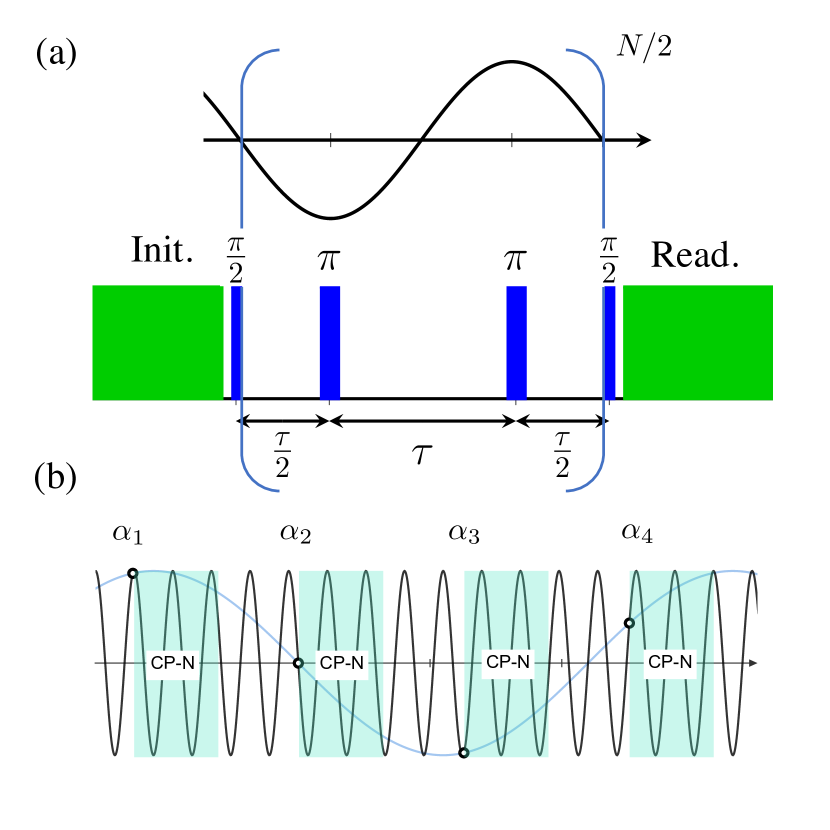
Figure 1: (a) Schematic of Carr-Purcell (CP) sequence under an AC field. The green and red boxes represent the laser and microwave pulses, respectively. (b) Schematic of sequential readout. The blue-shaded blocks marked “CP-N” represent the sequence shown in (a).

We describe our idea below. Figure 1(a) shows the CP sequence with the initialization/readout of the NV center. The state inversion by two $\pi$ pulses, repeated with a period of $T=2\tau$, forms the Floquet state as mathematically formulated in an analytical way [see Supplementary Information (SI)]. In the presence of a sinusoidal AC magnetic field with a frequency of $\omega_{\text{ac}}=\pi/\tau$, this Floquet state accumulates the precession phase given as

$$\phi_{\text{acq}}=2N\frac{\gamma b_{\text{ac}}}{\omega_{\text{ac}}}\cos(\phi_{\text{ac}}),$$ (1)

where $\gamma=2\pi\times 28~{}\mathrm{rad~{}GHz/T}$ is the gyromagnetic ratio of an NV center and $N$ is the number of $\pi$ pulses. $b_{\text{ac}}$ and $\phi_{\text{ac}}$ are the amplitude and phase of the AC field, respectively. We assume an ideal $\pi$ pulse without duration. The phase accumulation yields the probability ($P_{0}$) of the NV center returning to its initial state at the readout laser pulse as given by

$$P_{0}=\frac{1+\sin\phi_{\text{acq}}}{2}=\frac{1}{2}\quantity{1+\sin\quantity[2N\frac{\gamma b_{\text{ac}}}{\omega_{\text{ac}}}\cos(\phi_{\text{ac}})]}.$$ (2)

$P_{0}$ contains rich information on the phase dynamics of the Floquet state, which is intrinsically nonlinear to the AC field. Experimentally, $P_{0}$ can be estimated from the photoluminescence intensity of the NV center.

We note that since the CP sequence and the AC magnetic field exist simultaneously, both are treated as periodic driving. In this work, for clarity, we first extract the eigenstates of CP sequence as a basis and calculate the Floquet dynamics by the convolution of them and AC field modulation. For details, see SI.

We systematically investigate the response using the sequential readout technique. Figure 1(b) shows the protocol. By repeating the CP sequence in a fixed interval $t_{L}$, the phase of the AC field in each readout increases sequentially as $\alpha_{j}=\phi_{\text{ac}}+j\omega_{\text{ac}}t_{L}(j=0,1,2\cdots)$. The time-series data resulting in each readout contain multiple harmonics, whose amplitude can be obtained by the discrete Fourier transformation (DFT) of $P_{0}$. Specifically, as derived in SI, the DFT amplitude for $k$th harmonics at $\omega_{k}=k\omega_{\mathrm{ac}}$ is expressed as

$$A_{k}=J_{k}\quantity(2N\frac{\gamma b_{\text{ac}}}{\omega_{\text{ac}}}),$$ (3)

where $J_{k}$ denotes the $k$th order Bessel function of the first kind, and $k$ is odd positive integer.

Equation (3) describes the response reflecting the Floquet state dynamics in individual CP sequences. When the field amplitude is small (${b_{\text{ac}}\ll\frac{\omega_{\text{ac}}}{2N\gamma}\times\frac{\pi}{2}}$ or $\phi_{\text{acq}}\ll\pi/2$), only the first-order Bessel function takes finite values, and the field amplitude dependence remains linear. Higher-order Bessel functions emerge due to the nonlinear responses when the field amplitude becomes large. The degree to which the AC field amplitude is consistent with the DFT amplitude given by Eq. (3) is a crucial test of the robustness of this Floquet state for large amplitude modulation, which is the primary concern of the present work.

We describe our experimental condition. We measure a single NV center with a homemade confocal microscope [44]. We set the $\pi$ pulse duration to $t_{\pi}=19.8$ ns and the number of $\pi$ pulses to $N=16$ for the CP sequence. In this situation, the response of the Floquet state, created by $N/2=8$ cycles of the CP sequence, is observed as formulated in SI. The AC magnetic field of $\omega_{\mathrm{ac}}=2\pi\times 500.1$ kHz is generated by applying an AC voltage to a solenoid coil placed near the NV center. By increasing the voltage amplitude from $0.4$ mVpp to $300$ mVpp, the AC magnetic field with an amplitude up to $\sim 120~{}\mathrm{\mu T}$ is estimated to be produced, which is far beyond the small-amplitude regime ($b_{\text{ac}}\approx\frac{\omega_{\text{ac}}}{2N\gamma}\times\frac{\pi}{2}=877$ nT). We set the period of sequential readout as $t_{L}=2.0~{}\mathrm{\mu s}$ and measure $335.5$ seconds in total. In this condition, $k$th harmonics should appear at DFT frequency of $k\times 100$ Hz. For further experimental details, see SI.

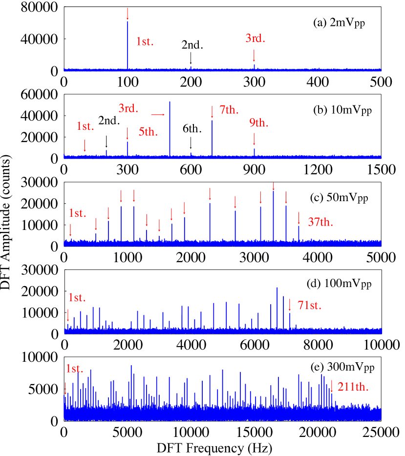
Figure 2: DFT spectra at several AC voltage amplitudes. (a) 2 mVpp, (b) 10 mVpp, (c) 50 mVpp, (d) 100 mVpp, and (e) 300 mVpp. A finite offset of about 3,000 counts due to photon shot noise is commonly present in all the data.

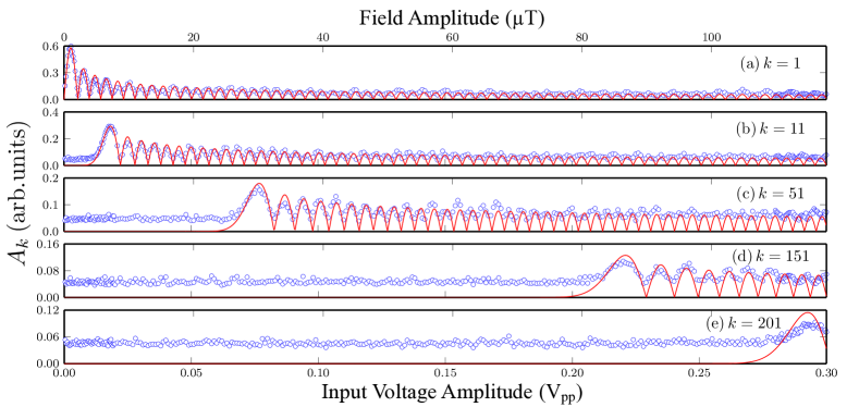
Figure 3: Input voltage amplitude dependence of the peak amplitude for (a) 1st, (b) 11th, (c) 51st, (d) 151st, and (e) 201st harmonics. The top axis show the magnetic field amplitude estimated from the fitting coefficient $0.392~{}\mathrm{\mu T/mVpp}$.

From here, we explain our experimental results. Figure 2(a) is the DFT spectrum obtained when the voltage amplitude to generate AC magnetic field is as small as 2 mVpp. There are a large peak at 100 Hz and a small peak at 300 Hz. These correspond to the harmonics of $k=1$ and $k=3$, respectively, and the absence of peaks higher than $k=3$ tells that the AC field amplitude is sufficiently small and the system is in the linear regime. This is a condition similar to those reported in the previous studies using the sequential readout [41, 42, 43]. Additionally, We see a peak at 200 Hz smaller than the peak at 300 Hz. This even harmonic is caused by a pulse error (see SI). The present high-frequency resolution achieved by sequential readout allows the detection of such a small signal.

We then show the modulation voltage amplitude dependence of the DFT spectrum. Figures 2(a), (b), (c), (d), and (e) show the DFT spectra when voltage amplitudes of 2 mVpp, 10 mVpp, 50 mVpp, 100 mVpp, and 300 mVpp are applied, respectively. As seen in these figures, odd harmonics appear up to higher orders successively as the amplitude increases. In particular, even a peak for $k=211$ harmonic is observed in the spectrum for 300 mVpp in Fig. 2(e). Such a higher-order response has not been investigated with this high precision before. A finite offset of about 3,000 counts due to photon shot noise is commonly present in all the data in Figs. 2 (a)–(e).

Now, we quantitatively examine the amplitude of each harmonic by comparing it to the Bessel function [Eq. (3)]. Figures 3 (a), (b), (c), and (d) show the results for 1st, 11th, 51st, 151st, and 201st harmonics, respectively. The blue circles show the DFT amplitudes obtained by fitting the DFT spectra normalized to the state probabilities by the experimentally calibrated NV center’s photoluminescence intensity (see SI). The constant offset of about 0.05 present in each figure is an artifact in the peak analysis due to the photon shot noise mentioned above. The solid red lines show the analytical results fitted by Eq. (3), reasonably assuming that the voltage amplitude and AC magnetic field amplitude are proportional and using only its proportionality coefficient as a fitting parameter. The obtained coefficient is $0.392~{}\mathrm{\mu T/mVpp}$, consistent with another AC magnetometry without using a sequential readout [see Fig. S1 in SI for technical details]. We find that both the experimental and theoretical [Eq. (3)] oscillation periods and amplitudes are in general agreement, even up to higher-order harmonics exceeding 200. These results mean that the Floquet state of the pulse-driven NV center is maintained even in large-amplitude modulation. It is also significant that each DFT amplitude is consistent with theory without any artificial normalization; it indicates that the sequential readout contributes to a highly quantitative measurement.

The AC field amplitude in the present experiment ranges from $157~{}\mathrm{nT}$ at minimum to $118~{}\mathrm{\mu T}$ at maximum, confirming that our investigation is systematic over a wide amplitude range, from near the linear response regime to a highly nonlinear nonequilibrium regime. Although similar experiments in previous studies have observed the response to be a Bessel function [45] and the appearance of multiple harmonics [46], we find that the peak amplitudes are quantitatively consistent over a significantly more extensive amplitude range than those. While large-amplitude modulation in different physical phenomena can give dynamics that exhibit Bessel functions [26, 7], Bessel functions of as high as 200 orders have never been observed experimentally, which means that our idea to use sequential readout for the NV center is relevant in studying Floquet state dynamics in a large-amplitude modulation.

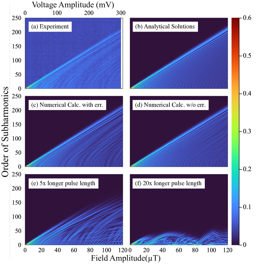
Figure 4: Two-dimensional intensity plots of the peak amplitude as functions of the AC field amplitude and the harmonics ($k$) up to 250. The color scale is common for all the panels (a)–(f). (a) Experimental result. (b) Analytical result [Eq. (3)]. (c-f) (c) Numerical result including finite pulse duration with the duration error of 4 % ($-0.8$ ns). (d) Numerical result including finite pulse duration without the duration error. (e) Numerical result considering $5\times$ longer duration than the present experiment ($t_{\pi}=100$ ns). (f) Numerical result considering $20\times$ longer duration than the present experiment ($t_{\pi}=400$ ns).

We now present an overall comparison of the theoretical calculations with the AC field amplitude dependence of all experimentally observed harmonics. Figure 4(a) shows the intensity plot of the experimental result as functions of the field amplitude and the order of harmonics ($k$). Figure 4(b) shows the corresponding theoretical prediction deduced from Eq. (3). These figures are almost consistent, indicating that Eq. (3) can, in principle, explain all harmonic behaviors observed in this experiment.

A more careful comparison reveals irregular fluctuations in the experimental intensity [Fig. 4(a)], which is not present in Fig. 4(b). We compare this behavior with a more detailed physical model that includes finite pulse duration and errors. Figures 4(c) and (d) show the numerical results considering finite pulse duration with and without the duration error of 4 % ($-0.8$ ns), respectively. Both show irregular fluctuations, and in particular, the result in Fig. 4(c) agrees very well with the experimental results [Fig. 4(a)]. These observations suggest a slight inevitable pulse error in the experiment. This fact also explains the appearance of the small even-order harmonics in Fig. 2. Such a small pulse error can appear by the rise and fall times of the rectangular pulses used in the CP sequence.

Further numerical calculations show that the bandwidth of the pulse excitation limits the measurable amplitude range. Figures 4(e) and (f) show the numerical calculations for $t_{\pi}=100$ ns and $t_{\pi}=400$ ns, respectively. The respective pulse durations are 5 and 20 times longer than that used in the present experiment ($t_{\pi}=19.8$ ns). As shown Fig. 4(e) and (f), the longer the pulse duration, the more irregular fluctuations appear, and the higher-order harmonics are no longer observable. This is because the bandwidth of the pulse excitation ($1/t_{\pi}$) gets narrower than the range of the NV center’s resonance frequency modulation. We observe that the amplitude of the higher-order harmonics does not appear finite in the area where the AC field amplitude is large, i.e., larger than that around 80 µT in Fig. 4(e) and around 20 µT in Fig. 4(f). There, the driving force by AC field exceeds the microwave pulse driving and breaks down the pulse driven Floquet state (see SI).

We discuss two significant implications of the present result for Floquet engineering. First, based on the above development, we can largely extend the modulation amplitude range available for Floquet engineering, such as quantum sensing [17, 47, 48, 49, 18]. For example, the demonstrated method is advantageous in observing dressed states [50, 49, 47, 51] and many-body states formed by interactions with surrounding spins  [11, 12]. The pulse-driven NV center can also be helpful as a robust Floquet state in evaluating the effects of finite pulse duration or error in general two-level systems [52, 53, 54, 55, 13]. Second, exploring the non-Hermitian Floquet dynamics is a promising direction. In the present experiment, the CP sequence readout completely initializes the NV center, quenching the Floquet state. Conversely, the sequential readout with partial initialization or weak measurement of the NV center and surrounding nuclear spins [56, 57] would serve as a platform to investigate non-Hermitian Floquet dynamics [58, 15].

In summary, we precisely observed the dynamics of the NV center’s Floquet state driven by the CP sequence in large-amplitude modulation as the higher-order harmonics up to 211 by using the sequential readout technique. We have thus established the relevance of the high precision of the sequential readout in Floquet engineering. The nonlinear response of the Floquet state to the magnetic field is quantitatively reproduced by numerical simulations, including the effects of finite pulse duration or error. This study further enhances the potential of the NV center as an ideal platform for Floquet engineering.

We thank Takashi Oka and Naoto Tsuji for helpful discussion, and Takuya Isogawa for assistance in early experiments. This work was supported by Forefront Physics and Mathematics Program to Drive Transformation (FoPM), a World-leading Innovative Graduate Study (WINGS) Program, the University of Tokyo, and by Grants-in-Aid for Scientific Research Nos. JP19H00656, JP19H05826, JP20K22325, JP18H01502, JP22H01558, and JP19H02547, and by Q-LEAP (No. JPMXS0118067395), and by Center for Spintronics Research Network, Keio University.

I Supplementary Information

I.1 Setups

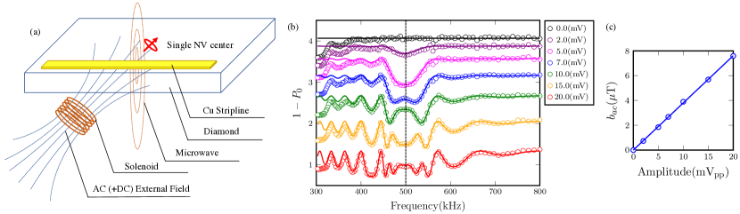
Figure 5: (a) Schematic of our experimental setup. (b) AC magnetometry using CP sequence. The target AC magnetic field frequency is 500.1 kHz. For clarity, the data of each conditions are shifted vertically. (c) The relation between input voltage amplitude and AC field amplitude obtained from the fitting of (b).

Figure 5(a) is the schematic of our experimental setup. We measure a single NV center in IIa diamond substrate (of electrical grade from Element Six) using a homemade confocal system [44]. We apply a static bias magnetic field of around 30 mT by a Neodymium magnet beneath the diamond [not shown in Fig. 5(a)] to lift the spin degeneracy of the energy levels. For the generation of microwave field to control the NV center, we use a copper stripline approximately $1~{}\mu$m-thick and $200~{}\mu$m-wide fabricated right on the surface of the diamond using electron-beam deposition. The microwave pulse waveform is generated by IQ modulation of a vector signal generator with an arbitrary waveform generator (AWG), amplified by an typ. +45 dB microwave amplifier (Mini-circuit ZHL-16W-43S+), and passed through the stripline. The AC external magnetic field is generated by the solenoid coil situated beneath the diamond as presented in Fig. 5(a). A function generator (FG) and typ. +43 dB amplifier (Mini-circuit LZY-22+) to generate a sinusoidal wave voltage at 500.1 kHz are connected to the coil and triggered by the AWG, which synchronizes the phase at the start of the sequential readout. The clocks of all the instruments are locked by a rubidium clock.

We check the linearity between the applied voltage amplitude of the FG and the resulting field amplitude $b_{\text{ac}}$ prior to the experiment described in the main text. We measure $b_{\text{ac}}$ with AC magnetometry by sweeping the interpulse delay $\tau$ of the Carr-Purcell (CP) sequence [30]. Only in this measurement do we randomize the phase of the AC magnetic field. The obtained spectra for applied voltage amplitude $0.0,2.0,5.0,7.0,10.0,15.0$, and $20.0$ mVpp are shown in Fig. 5(b). The horizontal axis is the detection frequency $1/2\tau$, and the vertical axis is the transition probability of the NV center. As the voltage is increased, a signal appears near 500.1 kHz. We fit the data with the analytical model [59],

$$P_{0} =\frac{1}{2}(1-J_{0}(|W_{a}|\gamma b_{ac}N\tau)),$$

$$W_{a} =\frac{\sin(\omega_{\text{ac}}N\tau/2)}{\omega_{\text{ac}}N\tau/2}\quantity(1-\frac{1}{\mathrm{cos}(\omega_{\text{ac}}\tau/2)}),$$ (4)

where $N$ is the number of $\pi$ pulses and $J_{0}$ is the 0-th order Bessel function. The fitted spectra are shown as the solid lines in Fig. 5(b). The model nicely explains the experimental data for all the input voltage amplitudes. Note that the small difference between the experimental data and the fitting at around 300 kHz is due to the effect of ${}^{13}\mathrm{C}$ nuclear spins near the present NV center. We exclude this region from the fitting to obtain $b_{\text{ac}}$ accurately.

The obtained relationship between applied voltage and magnetic field amplitude is shown in Fig. 5(c). We obtain excellent linearity, yielding a conversion factor of $0.381\pm 0.004~{}\mathrm{\mu T/mVpp}$. The results in the main text are obtained with the same NV center using the same setup shown here. The conversion factor obtained from the synchronized readout is $0.392~{}\mathrm{\mu T/mVpp}$, which is slightly larger than the above value. This is presumably due to the difference in the amplitude range and the effect of the quasi-cyclic distortion caused by the pulse error.

I.2 Principle of measurement of Floquet state by the sequential readout

We explain the definition of the Floquet state in the present study and the principle of measuring its response with sequential readout technique. For simpler interpretation, we devide the driving force into two parts, one by the CP sequence and the other by AC field modulation. We first extract the eigenstates of CP sequence as a basis. Then in order to calculate the total unitary operator including the AC field drive, we take the convolution of the time evolution of these eigenstates and AC field modulation.

This section is organized as follows. Sec.  I.2.1 defines the terms of Floquet theory [1, 2] relevant to this study. Sec. I.2.2 describes the Floquet states driven by the CP sequence. Sec. I.2.3 shows how that Floquet state is precessed by the AC field. Sec. I.2.4 shows the principle of phase readout of the Floquet state by the sequential readout technique. Sec. I.2.5 derives Eq. (3) in the main text and shows how to compare theory and experiment.

I.2.1 Floquet picture

When the Hamiltonian has periodicity such that $\hat{H}(t)=\hat{H}(t+T)$, the solution $\ket{\Psi_{F}(t)}$ of the following time-dependent Schrödinger equation ($\hbar=1$),

$$i\frac{\partial}{\partial t}\ket{\Psi_{\text{F}}(t)}=\hat{H}(t)\ket{\Psi_{\text{F}}(t)},$$ (5)

can be described by the Floquet theory. Accordingly, $\ket{\Psi_{F}(t)}$ can be expressed with periodic states $\ket{\Phi_{\alpha}(t+T)}=\ket{\Phi_{\alpha}(t)}$ in the following form:

$$\ket{\Psi_{\text{F}}(t)}=\sum_{\alpha}c_{\alpha}e^{i\epsilon_{\alpha}t}\ket{\Phi_{\alpha}(t)},\quad c_{\alpha}\in\mathbb{C}$$ (6)

Here, we call $\ket{\Psi_{\text{F}}(t)}$ Floquet state, $\ket{\Phi_{\alpha}(t)}$ Floquet mode, and $\epsilon_{\alpha}$ quasienergy. The Floquet mode and quasienergy are determined by the following eigenvalue problem of time-independent Floquet Hamiltonian $\hat{\mathcal{H}}_{\alpha}$,

$$\hat{\mathcal{H}}_{\alpha} =\hat{H}(t)-i\frac{\partial}{\partial t},$$ (7)

$$\hat{\mathcal{H}}_{\alpha}\ket{\Phi_{\alpha}(t)} =\epsilon_{\alpha}\ket{\Phi_{\alpha}(t)}.$$ (8)

The periodicity of the Floquet mode straightforwardly explains the stroboscopic response of the Floquet state of the period $T$, and such formalism opens up an easy understanding of a periodically driven system.

I.2.2 Floquet state driven by CP sequence

We consider the $m_{S}=0$ and $-1$ states of the NV center in a static magnetic field, which is a two-level system as treated in the present experiment. We express them as $\ket{0}$ and $\ket{1}$, respectively. We assume that the microwave pulse is rectangular and resonant to the NV center. The Hamiltonian for the CP sequence in the rotational coordinate system under the rotating wave approximation is given as,

$$\hat{H}^{\mathrm{CP}}(t) =\begin{cases}\Omega_{\text{R}}\hat{S}(\phi_{1})&\frac{\tau-t_{\pi}}{2}+2n\tau\leq t<\frac{\tau+t_{\pi}}{2}+2n\tau\\ \Omega_{\text{R}}\hat{S}(\phi_{2})&\frac{3\tau-t_{\pi}}{2}+2n\tau\leq t<\frac{3\tau+t_{\pi}}{2}+2n\tau\\ 0&\mathrm{otherwise},\end{cases}\quad\text{for}~{}n=0,1,\cdots,(N/2-1)$$ (9)

where $\Omega_{R}=\frac{\pi}{t_{\pi}}$ is the Rabi frequency, $\hat{S}(\phi_{i})=\frac{1}{2}(e^{i\phi_{i}}\ket{1}\bra{0}+e^{-i\phi_{i}}\ket{0}\bra{1})$, $\phi_{i}$ is the pulse phase ($i=1,2$), $t_{\pi}$ is the $\pi$ pulse duration, $\tau$ is the interpulse delay and $N$ is the number of $\pi$ pulses.

The Hamiltonian Eq. (9) should be modified according to the pulse phase series used in the CP sequence. For a technical reason, we first consider the finite pulse duration $t_{\pi}$. Since it has a periodicity of $T=2\tau$, a quantum state under the Hamiltonian is a Floquet state. When the initial state is $\ket{\psi_{0}(t=0)}=\ket{0}$, the time evolution in one cycle $t=[0,2\tau]$ of the CP sequence is obtained as,

$$\ket{\psi_{0}(t)} =\begin{cases}\ket{0}&0\leq t<\frac{\tau-t_{\pi}}{2}\\ \hat{U}_{p}(\phi_{1},t,\frac{\tau-t_{\pi}}{2})\ket{0}&\frac{\tau-t_{\pi}}{2}\leq t<\frac{\tau+t_{\pi}}{2}\\ -ie^{-i\phi_{1}}\ket{1}&\frac{\tau+t_{\pi}}{2}\leq t<\frac{3\tau-t_{\pi}}{2}\\ -ie^{-i\phi_{1}}\hat{U}_{p}(\phi_{2},t,\frac{3\tau-t_{\pi}}{2})\ket{1}&\frac{3\tau-t_{\pi}}{2}\leq t<\frac{3\tau+t_{\pi}}{2}\\ -e^{-i(\phi_{1}-\phi_{2})}\ket{0}&\frac{3\tau+t_{\pi}}{2}\leq t<2\tau,\end{cases}$$ (10)

where $\hat{U}_{p}(\phi,t_{f},t_{i})$ is the pulse operation during $t\in[t_{i},t_{f}]$ with phase $\phi$, which is given as

$$\hat{U}_{p}(\phi,t_{f},t_{i})=\exp[-i\frac{\pi}{t_{\pi}}(t_{f}-t_{i})\hat{S}(\phi)]=\cos\quantity[\frac{\pi}{2t_{\pi}}(t_{f}-t_{i})]\bm{1}-2i\sin\quantity[\frac{\pi}{2t_{\pi}}(t_{f}-t_{i})]\hat{S}(\phi).$$ (11)

The state $\ket{\psi_{0}(t)}$ is an eigenstate of the Hamiltonian Eq. (9), satisfying Eq. (5), and therefore a Floquet state. Similarly, the state

$$\ket{\psi_{1}(t)}=(\ket{1}\bra{0}+\ket{0}\bra{1})\ket{\psi_{0}(t)},$$ (12)

which is orthogonal to $\ket{\psi_{0}(t)}$ is also a Floquet state. These two states are in nature normalized and orthogonal to each other. Futhermore, the basis of these two states $\ket{\psi_{0}(t)}$ and $\ket{\psi_{1}(t)}$ span the whole Floquet state represented in Eq. (6).

The global phase offset $\phi_{1}-\phi_{2}+\pi$ is accumulated to the quantum state every cycle of the CP sequence as in Eq. (10). This does not change the observables in this two-level system. Thus, for simplicity, we fix the pulse phase condition to be $\phi_{1}-\phi_{2}+\pi=0$ for $\ket{\psi_{0}(t)}$ and $\ket{\psi_{1}(t)}$, which results in $\ket{\Phi_{0}^{\mathrm{CP}}(t)}$ and $\ket{\Phi_{1}^{\mathrm{CP}}(t)}$, respectively. They satisfy the following periodic condition,

$$\ket{\Phi_{0}(t+2\tau)^{\mathrm{CP}}} =\ket{\Phi_{0}^{\mathrm{CP}}(t)},$$ (13)

$$\ket{\Phi_{1}(t+2\tau)^{\mathrm{CP}}} =\ket{\Phi_{1}^{\mathrm{CP}}(t)}.$$ (14)

These states are Floquet modes in Eq. (6) with quasienergy $\epsilon_{\alpha}^{\mathrm{CP}}=0$. With these Floquet modes, the Floquet state $\ket{\Psi_{\text{F}}(t)}$ is expressed by using appropriate coefficients $c_{0}^{\prime}$ and $c_{1}^{\prime}$ such that

$$\ket{\Psi_{\text{F}}(t)}=c_{0}^{\prime}\ket{\Phi_{0}^{\mathrm{CP}}(t)}+c_{1}^{\prime}\ket{\Phi_{1}^{\mathrm{CP}}(t)}.$$ (15)

Now, without losing the essence of the Floquet picture, we can set the $\pi$ pulse duration $t_{\pi}\to 0$. The CP pulse Hamiltonian Eq. (9) can be rewritten using the Dirac delta $\delta(t)$ as,

$$\hat{H}^{\mathrm{CP}}(t)=\pi\delta(t-\tau/2)\hat{S}(\phi_{1})+\pi\delta(t-3\tau/2)\hat{S}(\phi_{2}).$$ (16)

Accordingly, the Floquet modes of the CP sequence are represented as the eigenstates of $\hat{H}^{\mathrm{CP}}(t)$ such that

$$\ket{\Phi_{0}^{\mathrm{CP}}(t)} =\frac{1-h(t)}{2}\ket{0}+\frac{1+h(t)}{2}\ket{1},$$ (17)

$$\ket{\Phi_{1}^{\mathrm{CP}}(t)} =\frac{1+h(t)}{2}\ket{0}+\frac{1-h(t)}{2}\ket{1},$$ (18)

where $h(t)$ is the modulation function

$$h(t) =\begin{cases}-1&0<t<\frac{\tau}{2},\quad\frac{3\tau}{2}<t<2\tau\\ 1&\frac{\tau}{2}<t<\frac{3\tau}{2}.\end{cases}$$ (19)

as depicted in Fig.6(b).

Eqs. (10) and (12) tell that the pulse phases, $\phi_{1}$ and $\phi_{2}$, do not affect the total dynamics of the Floquet state other than the global phase, we can arbitrarily choose them. We set the phase cycle as XY8 to reduce experimental pulse error. Figure 6(a) shows the phase cycle that we adopt in our experiment.

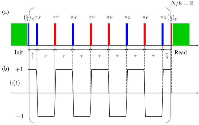
Figure 6: (a) Diagram of the pulse cycle (XY8) that we adopt in our experiment. We use $N=16$.(b) Modulation function $h(t)$ over time.

I.2.3 Precession of the Floquet state driven by CP sequence in the AC magnetic field

We consider the case where an arbitrary AC magnetic field $f(t)$ is applied in the direction of the symmetry axis of the NV center. Generally, a periodic function $f(t)$ with a period $T=2\tau$ can be expanded in the Fourier series as,

$$f(t)=a_{0}+\sum_{k=1}^{\infty}\quantity[a_{k}\cos(k\omega t)+b_{k}\sin(k\omega t)],$$ (20)

where $\omega=\pi/\tau$. A Hamiltonian under the AC magnetic field is given in the Hilbert space that the spin operator basis spans:

$$\hat{H}^{\mathrm{AC}}(t)=f(t)\ket{1}\bra{1}.$$ (21)

The total Hamiltonian for the Floquet state driven by CP sequence in the AC magnetic field is given by

$$\hat{H}_{\text{tot}}(t)=\hat{H}^{\mathrm{AC}}(t)+\hat{H}^{\mathrm{CP}}(t),$$ (22)

which is represented in the same basis. We write down the above Hamiltonian in the basis of the CP Floquet mode $\ket{\Phi_{i}(t)^{(\text{CP})}}$ in Eqs. (17) and (18). In this frame the pulse operation Hamiltonian $\hat{H}^{\mathrm{CP}}(t)$ vanishes and the total Hamiltonian $\breve{H}_{\text{tot}}(t)$ ($~{}\breve{}$ denotes the frame transformation) is

$$\breve{H}_{\text{tot}}(t)=\hat{H}^{\mathrm{AC}}(t)=f(t)\quantity(\frac{1+h(t)}{2}\ket{\Phi_{0}^{\mathrm{CP}}(t)}\bra{\Phi_{0}^{\mathrm{CP}}(t)}+\frac{1-h(t)}{2}\ket{\Phi_{1}^{\mathrm{CP}}(t)}\bra{\Phi_{1}^{\mathrm{CP}}(t)}).$$ (23)

In the above, we have utilized the following identity:

$$\quantity(\frac{1\pm h}{2})^{2}=\frac{1\pm h}{2},\quad\quantity(\frac{1+h}{2})\quantity(\frac{1-h}{2})=0.$$ (24)

Note that this expression is equivalent to applying the following unitary transformation to $\hat{H}_{\text{tot}}(t)$. The unitary operator $\hat{U}_{t}$ to represent this frame conversion is

(25)

The identity

$$i\frac{\partial\hat{U}_{t}}{\partial t}(t)\hat{U}_{t}^{\dagger}(t)=\hat{H}^{\mathrm{CP}}(t)$$ (26)

holds from the fact that $\ket{\Phi_{0}^{\mathrm{CP}}(t)}$ and $\ket{\Phi_{1}^{\mathrm{CP}}(t)}$ are the orthonormal eigenstates of $\hat{H}^{\mathrm{CP}}(t)$ [Eq. (16)] that satisfy time-dependent Shrödinger equation (5). The following identity of the unitary operation

$$\hat{H}_{\text{tot}}(t)=\hat{U}_{t}(t)^{\dagger}\breve{H}_{\text{tot}}(t)\hat{U}_{t}(t)+i\frac{\partial\hat{U}^{\dagger}_{t}}{\partial t}(t)\hat{U}_{t}(t)$$ (27)

holds.

In the presence of the AC field, each Floquet mode is in precession with the frequency given as,

$$\xi_{0}^{\mathrm{CP}}(t)=f(t)\frac{1+h(t)}{2},\quad\xi_{1}^{\mathrm{CP}}(t)=f(t)\frac{1-h(t)}{2}.$$ (28)

Only the components of the AC field filtered by the modulation function $h(t)$ is acquired as the precession phase. The phase acquisition during $t=[0,2\tau]$, $\phi_{u}$, is obtained by the convolution $(h*f)(2\tau)=\int_{0}^{2\tau}h(2\tau-t^{\prime})f(t^{\prime})dt^{\prime}$ as,

$$\phi_{u}=\int_{0}^{2\tau}\xi_{0}^{\mathrm{CP}}(t)dt=-\int_{0}^{2\tau}\xi_{1}^{\mathrm{CP}}(t)dt=\sum_{j=0}^{\infty}a_{2j+1}\frac{2(-1)^{j}}{(2j+1)\omega},$$ (29)

Here, we use the symmetry $h(t)=h(2\tau-t)$ and the Fourier series of $h(t)$ given as,

$$h(t)=\sum_{j=0}^{\infty}\frac{4}{\pi}\frac{(-1)^{j}}{(2j+1)}\cos[(2j+1)\omega t].$$ (30)

Since $h(t)$ consists only of odd-order cosine part of the Fourier composition, only the matched components of $f(t)$ contribute to the dynamics, as derived from the property of the convolution. The dynamics $\hat{U}$ in the overall sequence $t=[0,2\tau N]$ is obtained as,

$$\hat{U} =e^{+iN\phi_{u}/2}\ket{\Phi_{0}^{\mathrm{CP}}(t)}\bra{\Phi_{0}^{\mathrm{CP}}(t)}+e^{-iN\phi_{u}/2}\ket{\Phi_{1}^{\mathrm{CP}}(t)}\bra{\Phi_{1}^{\mathrm{CP}}(t)}$$ (31)

and here,

$$\phi_{\text{acq}}=N\phi_{u}$$ (32)

is the net phase acquisition of the Floquet states. In the stroboscopic measurement at the end of the CP sequence, the state $\ket{0}(\ket{1})$ is not experimentally distinguished from the state $\ket{\Phi_{0}^{\mathrm{CP}}(t)}(\ket{\Phi_{1}^{\mathrm{CP}}(t)})$.

Thus we have described the Floquet engineering used as AC magnetometry. The Floquet state dynamics is explained by the convolution of the modulation function $h(t)$ and the target AC field $f(t)$. CP sequence can be understood as engineering to extract only the cosine of the odd harmonic components of $f(t)$ as in Eq. (29). By designing the modulation function by adjusting $\tau$ appropriately, it is possible to extract any frequency components of the AC field.

I.2.4 Principle of measuring the phase dynamics of a Floquet state by sequential readout technique

From now on, we describe how to obtain the phase dynamics of the Floquet state driven by the CP sequence in the AC magnetic field. The dynamics is reflected in the phase acquisition $\phi_{\text{acq}}$. We use the initial state

$$\ket{\Psi_{\text{F}}(t=0)}=\left(\ket{\Phi_{0}^{\mathrm{CP}}(t=0)}-i\ket{\Phi_{1}^{\mathrm{CP}}(t=0)}\right)/\sqrt{2}=(\ket{0}-i\ket{1})/\sqrt{2}$$ (33)

to interferometrically measure the difference of the phase acquisition in the Floquet modes [See Eq. (15)]. By setting the phase of the $\pi/2$ pulse for the readout as $\phi=\frac{\pi}{2}$, the probability of detecting the NV center as $\ket{0}$ is obtained as,

$$P_{0} =\frac{1+\sin\phi_{\text{acq}}}{2}.$$ (34)

Thus, the phase accumulation is experimentally accessible by probing $P_{0}$.

We systematically investigate $\phi_{\text{acq}}$ by using sequential readout technique. In this technique, the CP sequence is repeated at a time interval of $t_{L}$. We redefine the time origin $t$ as the timing of the first CP sequence of the sequential readout; the start time of the $m$th CP sequence ($m=1,2,3,\cdots$) is $t_{m}=(m-1)t_{L}$. The time shift in the CP sequences causes a systematic AC field phase shift [Eq. (20)] such that

$$f(t+t_{m}) =a_{0}+\sum_{k=1}^{\infty}\quantity[a_{k}\cos(k\omega t_{m})+b_{k}\sin(k\omega t_{m})]\cos(k\omega)+\quantity[-a_{k}\sin(k\omega t_{m})+b_{k}\cos(k\omega t_{m})]\sin(k\omega).$$ (35)

Then, $\phi_{\text{acq}}(t_{m})$ in the $m$th CP sequence is obtained as

$$\phi_{\text{acq}}(t_{m}) =\sum_{j=0}^{\infty}\frac{2N(-1)^{j}}{(2j+1)\omega}\quantity{a_{2j+1}\cos[(2j+1)\omega t_{m}]+b_{2j+1}\sin[(2j+1)\omega t_{m}]}.$$ (36)

The Fourier series for $t_{m}$ of $\phi_{\text{acq}}(t_{m})$ contains all the odd harmonic components of $f(t)$. We can obtain each odd harmonic component of $f(t)$ as the spectrum of the time-series readout result $\quantity{P_{0}(t_{m})}$.

I.2.5 Method to compare theory and experiment

In our experiment, we observe the dynamics in the simplest sinusoidal AC magnetic field. Specifically, it corresponds to the case where all the Fourier series components except for $k=1$ in Eqs. (20,35) are zero,

$$f(t)=\gamma b_{\text{ac}}\cos(\omega_{\text{ac}}t+\phi_{\text{ac}})=\gamma b_{\text{ac}}\cos(\phi_{\text{ac}})\cos(\omega_{\text{ac}}t)-\gamma b_{\text{ac}}\sin(\phi_{\text{ac}})\sin(\omega_{\text{ac}}t)$$ (37)

where $b_{\text{ac}}$, $\omega_{\text{ac}}(=\pi/\tau)$, and $\phi_{\text{ac}}$ are the amplitude, frequency, and phase of the AC field, respectively. According to Eqs. (29) and (32), the phase acquisition at the $m$th CP sequence is obtained as,

$$\phi_{\text{acq}}(t_{m})=\frac{2N\gamma b_{\text{ac}}}{\omega_{\text{ac}}}[\cos\,\phi_{\text{ac}}\cos(\omega_{\text{ac}}t_{m})-\sin\,\phi_{\text{ac}}\sin(\omega_{\text{ac}}t_{m})]=\frac{2N\gamma b_{\text{ac}}}{\omega_{\text{ac}}}\cos(\omega_{\text{ac}}t_{m}+\phi_{\text{ac}})$$ (38)

The signal at the $m$th readout is obtained as,

$$P_{0}(t_{m}) =\frac{1+\sin[\frac{2N\gamma b_{\text{ac}}}{\omega_{\text{ac}}}\cos(\omega_{\text{ac}}t_{m}+\phi_{\text{ac}})]}{2}=\frac{1+\mathrm{Im}\quantity[\exp(i\frac{2N\gamma b_{\text{ac}}}{\omega_{\text{ac}}}\cos(\omega_{\text{ac}}t_{m}+\phi_{\text{ac}}))]}{2}$$ (39)

The Fourier series expansion of the signal for $t_{m}$ is obtained as,

$$P_{0}(t_{m}) =\frac{1}{2}+\sum_{k:\text{odd}}A_{k}\cos(k\omega_{\text{ac}}t_{m}+\phi_{k}),$$ (40)

$$A_{k} =J_{k}\quantity(2N\frac{\gamma b_{\text{ac}}}{\omega_{\text{ac}}}),$$ (41)

$$\phi_{k} =k\quantity(\frac{N\pi}{2}+\phi_{\text{ac}}-\frac{\pi}{2})-\frac{\pi}{2},$$ (42)

where $J_{k}$ is a Bessel function of the first kind of $k$th order. Here, we use the Jacobi–Anger identity

$$e^{ia\cos\varphi}=\sum_{n\in\mathbb{Z}}i^{n}J_{n}(a)e^{in\varphi}$$ (43)

The Fourier components obtained here correspond to Eq. (3) in the main text. The frequency resolution of the discrete Fourier transformation (DFT) spectrum can be set arbitrarily by the inverse of the total duration of sequential readout. Thus, with high accuracy, we can investigate the response that is dependent on the amplitude and phase of the AC field. According to Eq. (41), higher-order Bessel functions take non-zero value when the magnetic field amplitude increases. For a sufficiently weak magnetic field, the behavior of the $A_{k}$ is linear to $b_{ac}$. Specifically, we define the threshold as,

$$b_{ac}\approx\frac{\pi}{2}\frac{\omega_{ac}}{2N\gamma}=877\,\mathrm{nT}$$ (44)

I.3 Analysis of the experimental data

This section gives the procedure to extract the amplitude of the DFT peaks. We perform the fitting of the DFT spectrum, taking into account that the peaks of the data have a finite linewidth. Due to the finite time window of the measurement, we should assume the time series data as following form:

$$p(t)=Ae^{i(\omega t+\phi)}\quad t\in[0,T_{\text{tot}}],$$ (45)

where $T_{\mathrm{tot}}$ is the total duration of the sequential readout. This signal can be Fourier transformed as,

$$\mathcal{F}[p](\xi) =\int_{0}^{T_{\text{tot}}}p(t)e^{-i\xi t}dt=\frac{AT_{\text{tot}}}{4}e^{i\phi-i(\xi-\omega)T_{\text{tot}}/2}\times\mathrm{sinc}\quantity[(\xi-\omega)T_{\text{tot}}/2],$$ (46)

where $\mathrm{sinc}(x)\stackrel{{\scriptstyle\text{def}}}{{=}}\sin x/x$. Eq. (46) means that the DFT peak has a shape that broadens with a sinc function. We estimate the DFT peak amplitude by fitting the DFT spectrum with the peak shape represented by Eq. (46).

Figure 7(a) shows the intensity plot obtained using the above method (exactly the same as Fig. 4(a) in the main text). On the other hand, Fig. 7(b) shows the plot obtained simply by extracting the data at the frequency index closest to the $k$ th peak frequency in the DFT spectrum. In Fig.7(a), a smooth image is obtained, but in Fig.7(b), there is an artifact where the peak amplitude becomes smaller in certain period over $k$. This is an artifact due to the mismatch between the exact peak frequency and the frequency point of the DFT spectrum limited by the frequency resolution $1/T_{\mathrm{tot}}$. The above-described method allows accurate determination of the peak amplitude.

After obtaining the DFT peak values, we normalize the time series data obtained from sequential readouts for quantitative comparisons with theoretical models. Using the photoluminescence intensity $I_{0}$ (count/sec) of the $m_{S}=0$ state and $I_{1}$ (count/sec) of the $m_{S}=-1$ state at the NV center as reference data, we normalize the DFT amplitudes (count) to the dimensionless value of $A_{k}$ [44]. Specifically, the conversion of the scaling is given as,

$$\text{(DFT Amp.)}=(N_{\text{seq}}(I_{0}-I_{1})t_{\text{read}}/2)A_{k}.$$ (47)

$t_{\text{read}}$ is the readout duration (sec) and $N_{\text{seq}}$ is the total number of CP sequence repetition.

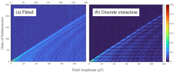
Figure 7: Intensity map of the DFT peak amplitude. (a) Analyzed result with our fitting method, which is the same figure shown in Fig. 4(a) in the main text. (b) The peak amplitude of the closest frequency point for $k$th harmonic.

I.4 Effect of the pulse error and finite pulse duration

We consider the effects of finite pulse duration. First, we consider the pulse error in the $\pi/2$ pulse. When the rotation angle of the pulse is $\pi/2+\epsilon$, Eq. (34) is rewritten as,

$$P_{0}\approx\frac{1}{2}(1+\sin\phi_{\text{acq}}-\epsilon\cos\phi_{\text{acq}}).$$ (48)

Compared to Eq. (2) in the main text, the pulse error occurs as a cosine term. This term appears as an effect that produces even-order harmonics of the DFT spectrum of the sequential readout [see Fig. 2(a) in the main text].

Next, we consider the effects of finite pulse duration and error in $\pi$ pulses. Since these effects can produce a variety of effects [52, 53, 54, 55, 13], we numerically investigate the situation to reproduce experimental observation. Specifically, we solve the time-dependent Schrödinger equation Eq. (5) of the total Hamiltonian $\hat{H}_{\text{tot}}(t)=\hat{H}^{\mathrm{AC}}(t)+\hat{H}^{\mathrm{CP}}(t)$ [Eq. (22)] with finite duration using the adaptive-step Runge-Kutta method. We adopt XY8 as the $\pi$ pulse phase cycle. The parameters of the Hamiltonian are all based on experimental data except the true Rabi frequency.

We show the results of these numerical simulations in Fig. 4(a) in the main text.

References

- Shirley [1965] J. H. Shirley, Phys. Rev. 138, B979 (1965).
- Sambe [1973] H. Sambe, Phys. Rev. A 7, 2203 (1973).
- Oka and Aoki [2009] T. Oka and H. Aoki, Phys. Rev. B 79, 081406 (2009).
- Malz and Smith [2021] D. Malz and A. Smith, Phys. Rev. Lett. 126, 163602 (2021).
- Martin et al. [2017] I. Martin, G. Refael, and B. Halperin, Phys. Rev. X 7, 041008 (2017).
- Eckardt [2017] A. Eckardt, Rev. Mod. Phys. 89, 011004 (2017).
- Weitenberg and Simonet [2021] C. Weitenberg and J. Simonet, Nat. Phys. 17, 1342 (2021).
- Oka and Kitamura [2019] T. Oka and S. Kitamura, Annu. Rev. Condens. Matter Phys. 10, 387 (2019).
- Haeberlen and Waugh [1968] U. Haeberlen and J. Waugh, Physical Review 175, 453 (1968).
- Choi et al. [2020] J. Choi, H. Zhou, H. S. Knowles, R. Landig, S. Choi, and M. D. Lukin, Phys. Rev. X 10, 031002 (2020).
- Choi et al. [2017] S. Choi, J. Choi, R. Landig, G. Kucsko, H. Zhou, J. Isoya, F. Jelezko, S. Onoda, H. Sumiya, V. Khemani, et al., Nature 543, 221 (2017).
- Randall et al. [2021] J. Randall, C. E. Bradley, F. V. van der Gronden, A. Galicia, M. H. Abobeih, M. Markham, D. J. Twitchen, F. Machado, N. Y. Yao, and T. H. Taminiau, Science 374, 1474 (2021).
- Zhou et al. [2020] H. Zhou, J. Choi, S. Choi, R. Landig, A. M. Douglas, J. Isoya, F. Jelezko, S. Onoda, H. Sumiya, P. Cappellaro, H. S. Knowles, H. Park, and M. D. Lukin, Phys. Rev. X 10, 031003 (2020).
- Zhang et al. [2017] J. Zhang, P. W. Hess, A. Kyprianidis, P. Becker, A. Lee, J. Smith, G. Pagano, I. D. Potirniche, A. C. Potter, A. Vishwanath, N. Y. Yao, and C. Monroe, Nature 543, 217 (2017).
- Beatrez et al. [2021] W. Beatrez, O. Janes, A. Akkiraju, A. Pillai, A. Oddo, P. Reshetikhin, E. Druga, M. McAllister, M. Elo, B. Gilbert, et al., Phys. Rev. Lett. 127, 170603 (2021).
- de Lange et al. [2011a] G. de Lange, D. Ristè, V. Dobrovitski, and R. Hanson, Phys. Rev. Lett. 106, 080802 (2011a).
- Lang et al. [2015] J. Lang, R.-B. Liu, and T. Monteiro, Phys. Rev. X 5, 041016 (2015).
- Meinel et al. [2021] J. Meinel, V. Vorobyov, B. Yavkin, D. Dasari, H. Sumiya, S. Onoda, J. Isoya, and J. Wrachtrup, Nat. Commun. 12, 2737 (2021).
- Ashhab et al. [2007] S. Ashhab, J. R. Johansson, A. M. Zagoskin, and F. Nori, Phys. Rev. A 75, 063414 (2007).
- Fuchs et al. [2009] G. Fuchs, V. Dobrovitski, D. Toyli, F. Heremans, and D. Awschalom, Science 326, 1520 (2009).
- Scheuer et al. [2014] J. Scheuer, X. Kong, R. S. Said, J. Chen, A. Kurz, L. Marseglia, J. Du, P. R. Hemmer, S. Montangero, T. Calarco, et al., New Journal of Physics 16, 093022 (2014).
- Rao and Suter [2017] K. R. K. Rao and D. Suter, Phys. Rev. A 95, 053804 (2017).
- Wang et al. [2021] G. Wang, Y.-X. Liu, P. Cappellaro, et al., Phys. Rev. A 103, 022415 (2021).
- Deng et al. [2015] C. Deng, J.-L. Orgiazzi, F. Shen, S. Ashhab, and A. Lupascu, Phys. Rev. Lett. 115, 133601 (2015).
- Dai et al. [2017] K. Dai, H. Wu, P. Zhao, M. Li, Q. Liu, G. Xue, X. Tan, H. Yu, and Y. Yu, Appl. Phys. Lett. 111, 242601 (2017).
- Saito et al. [2006] S. Saito, T. Meno, M. Ueda, H. Tanaka, K. Semba, and H. Takayanagi, Phys. Rev. Lett. 96, 107001 (2006).
- Oliver et al. [2005] W. D. Oliver, Y. Yu, J. C. Lee, K. K. Berggren, L. S. Levitov, and T. P. Orlando, Science 310, 1653 (2005).
- Berns et al. [2006] D. Berns, W. Oliver, S. Valenzuela, A. Shytov, K. Berggren, L. Levitov, and T. Orlando, Phys. Rev. Lett. 97, 150502 (2006).
- Berns et al. [2008] D. M. Berns, M. S. Rudner, S. O. Valenzuela, K. K. Berggren, W. D. Oliver, L. S. Levitov, and T. P. Orlando, Nature 455, 51 (2008).
- Kotler et al. [2013] S. Kotler, N. Akerman, Y. Glickman, and R. Ozeri, Phys. Rev. Lett. 110, 110503 (2013).
- Zopes et al. [2017] J. Zopes, K. Sasaki, K. S. Cujia, J. M. Boss, K. Chang, T. F. Segawa, K. M. Itoh, and C. L. Degen, Phys. Rev. Lett. 119, 260501 (2017).
- Niemczyk et al. [2010] T. Niemczyk, F. Deppe, H. Huebl, E. Menzel, F. Hocke, M. Schwarz, J. Garcia-Ripoll, D. Zueco, T. Hümmer, E. Solano, et al., Nat. Phys. 6, 772 (2010).
- Forn-Díaz et al. [2010] P. Forn-Díaz, J. Lisenfeld, D. Marcos, J. J. Garcia-Ripoll, E. Solano, C. Harmans, and J. Mooij, Phys. Rev. Lett. 105, 237001 (2010).
- Yoshihara et al. [2017a] F. Yoshihara, T. Fuse, S. Ashhab, K. Kakuyanagi, S. Saito, and K. Semba, Nat. Phys. 13, 44 (2017a).
- Yoshihara et al. [2017b] F. Yoshihara, T. Fuse, S. Ashhab, K. Kakuyanagi, S. Saito, and K. Semba, Phys. Rev. A 95, 053824 (2017b).
- Yoshihara et al. [2018] F. Yoshihara, T. Fuse, Z. Ao, S. Ashhab, K. Kakuyanagi, S. Saito, T. Aoki, K. Koshino, and K. Semba, Phys. Rev. Lett. 120, 183601 (2018).
- Maze et al. [2008] J. R. Maze, P. L. Stanwix, J. S. Hodges, S. Hong, J. M. Taylor, P. Cappellaro, L. Jiang, M. V. G. Dutt, E. Togan, A. S. Zibrov, A. Yacoby, R. L. Walsworth, and M. D. Lukin, Nature 455, 644 (2008).
- Hall et al. [2010] L. T. Hall, C. D. Hill, J. H. Cole, and L. C. L. Hollenberg, Phys. Rev. B 82, 045208 (2010).
- de Lange et al. [2011b] G. de Lange, D. Ristè, V. V. Dobrovitski, and R. Hanson, Phys. Rev. Lett. 106, 080802 (2011b).
- Naydenov et al. [2011] B. Naydenov, F. Dolde, L. T. Hall, C. Shin, H. Fedder, L. C. L. Hollenberg, F. Jelezko, and J. Wrachtrup, Phys. Rev. B 83, 081201 (2011).
- Schmitt et al. [2017] S. Schmitt, T. Gefen, F. M. Stürner, T. Unden, G. Wolff, C. Müller, J. Scheuer, B. Naydenov, M. Markham, S. Pezzagna, J. Meijer, I. Schwarz, M. Plenio, A. Retzker, L. P. Mcguinness, and F. Jelezko, Science 356, 832 (2017).
- Boss et al. [2017] J. M. Boss, K. S. Cujia, J. Zopes, and C. L. Degen, Science 356, 837 (2017).
- Glenn et al. [2018] D. R. Glenn, D. B. Bucher, J. Lee, M. D. Lukin, H. Park, and R. L. Walsworth, Nature 555, 351 (2018).
- Misonou et al. [2020] D. Misonou, K. Sasaki, S. Ishizu, Y. Monnai, K. M. Itoh, and E. Abe, AIP Advances 10, 025206 (2020).
- Mizuno et al. [2020] K. Mizuno, H. Ishiwata, Y. Masuyama, T. Iwasaki, and M. Hatano, Sci. Rep. 10, 11611 (2020).
- Barson et al. [2021] M. S. J. Barson, L. M. Oberg, L. P. Mcguinness, A. Denisenko, N. B. Manson, J. Wrachtrup, and M. W. Doherty, Nano Letters 21, 2962 (2021).
- Stark et al. [2017] A. Stark, N. Aharon, T. Unden, D. Louzon, A. Huck, A. Retzker, U. L. Andersen, and F. Jelezko, Nat. Commun. 8, 1 (2017).
- Saijo et al. [2018] S. Saijo, Y. Matsuzaki, S. Saito, T. Yamaguchi, I. Hanano, H. Watanabe, N. Mizuochi, and J. Ishi-Hayase, Appl. Phys. Lett. 113, 082405 (2018).
- Morishita et al. [2019] H. Morishita, T. Tashima, D. Mima, H. Kato, T. Makino, S. Yamasaki, M. Fujiwara, and N. Mizuochi, Sci. Rep. 9, 13318 (2019).
- Belthangady et al. [2013] C. Belthangady, N. Bar-Gill, L. M. Pham, K. Arai, D. Le Sage, P. Cappellaro, and R. L. Walsworth, Phys. Rev. Lett. 110, 157601 (2013).
- Stark et al. [2018] A. Stark, N. Aharon, A. Huck, H. A. El-Ella, A. Retzker, F. Jelezko, and U. L. Andersen, Sci. Rep. 8, 14807 (2018).
- Loretz et al. [2015] M. Loretz, J. M. Boss, T. Rosskopf, H. J. Mamin, D. Rugar, and C. L. Degen, Phys. Rev. X 5, 021009 (2015).
- Boss et al. [2016] J. M. Boss, K. Chang, J. Armijo, K. Cujia, T. Rosskopf, J. R. Maze, and C. L. Degen, Phys. Rev. Lett. 116, 197601 (2016).
- Ishikawa et al. [2019] T. Ishikawa, A. Yoshizawa, Y. Mawatari, S. Kashiwaya, and H. Watanabe, AIP Advances 9, 075013 (2019).
- Lang et al. [2017] J. E. Lang, J. Casanova, Z.-Y. Wang, M. B. Plenio, and T. S. Monteiro, Phys. Rev. Appl. 7, 054009 (2017).
- Pfender et al. [2019] M. Pfender, P. Wang, H. Sumiya, S. Onoda, W. Yang, D. B. R. Dasari, P. Neumann, X.-Y. Pan, J. Isoya, R.-B. Liu, and J. Wrachtrup, Nat. Commun. 10, 594 (2019).
- Cujia et al. [2019] K. Cujia, J. M. Boss, K. Herb, J. Zopes, and C. L. Degen, Nature 571, 230 (2019).
- Keßler et al. [2021] H. Keßler, P. Kongkhambut, C. Georges, L. Mathey, J. G. Cosme, and A. Hemmerich, Phys. Rev. Lett. 127, 043602 (2021).
- Degen et al. [2017] C. L. Degen, F. Reinhard, and P. Cappellaro, Rev. Mod. Phys. 89, 035002 (2017).