Multi-Agent Reinforcement Learning for Traffic Signal Control through Universal Communication Method

Abstract

How to coordinate the communication among intersections effectively in real complex traffic scenarios with multi-intersection is challenging. Existing approaches only enable the communication in a heuristic manner without considering the content/importance of information to be shared. In this paper, we propose a universal communication form UniComm between intersections. UniComm embeds massive observations collected at one agent into crucial predictions of their impact on its neighbors, which improves the communication efficiency and is universal across existing methods. We also propose a concise network UniLight to make full use of communications enabled by UniComm. Experimental results on real datasets demonstrate that UniComm universally improves the performance of existing state-of-the-art methods, and UniLight significantly outperforms existing methods on a wide range of traffic situations. Source codes are available at https://github.com/zyr17/UniLight.

1 Introduction

Traffic congestion is a major problem in modern cities. While the use of traffic signal mitigates the congestion to a certain extent, most traffic signals are controlled by timers. Timer-based systems are simple, but their performance might deteriorate at intersections with inconsistent traffic volume. Thus, an adaptive traffic signal control method, especially controlling multiple intersections simultaneously, is required.

Existing conventional methods, such as SOTL Cools et al. (2013), use observations of intersections to form better strategies, but they do not consider long-term effects of different signals and lack a proper coordination among intersections. Recently, reinforcement learning (RL) methods have showed promising performance in controlling traffic signals. Some of them achieve good performance in controlling traffic signals at a single intersection Zheng et al. (2019a); Oroojlooy et al. (2020); others focus on collaboration of multi-intersections Wei et al. (2019b); Chen et al. (2020).

Multi-intersection traffic signal control is a typical multi-agent reinforcement learning problem. The main challenges include stability, nonstationarity, and curse of dimensionality. Independent Q-learning splits the state-action value function into independent tasks performed by individual agents to solve the curse of dimensionality. However, given a dynamic environment that is common as agents may change their policies simultaneously, the learning process could be unstable and divergent.

To enable the sharing of information among agents, a proper communication mechanism is required. This is critical as it determines the content/amount of the information each agent can observe and learn from its neighboring agents, which directly impacts the amount of uncertainty that can be reduced. Common approaches include enabling the neighboring agents i) to exchange their information with each other and use the partial observations directly during the learning El-Tantawy et al. (2013), or ii) to share hidden states as the information Wei et al. (2019b); Yu et al. (2020). While enabling communication is important to stabilize the training process, existing methods have not yet examined the impact of the content/amount of the shared information. For example, when each agent shares more information with other agents, the network needs to manage a larger number of parameters and hence converges in a slower speed, which actually reduces the stability. As reported in Zheng et al. (2019b), additional information does not always lead to better results. Consequently, it is very important to select the right information for sharing.

Motivated by the deficiency in the current communication mechanism adopted by existing methods, we propose a universal communication form UniComm. To facilitate the understanding of UniComm, let’s consider two neighboring intersections $I_{i}$ and $I_{j}$ connected by a unidirectional road $R_{i,j}$ from $I_{i}$ to $I_{j}$. If vehicles in $I_{i}$ impact $I_{j}$, they have to first pass through $I_{i}$ and then follow $R_{i,j}$ to reach $I_{j}$. This observation inspires us to propose UniComm, which picks relevant observations from an agent $A_{i}$ who manages $I_{i}$, predicts their impacts on road $R_{i,j}$, and only shares the prediction with its neighboring agent $A_{j}$ that manages $I_{j}$. We conduct a theoretical analysis to confirm that UniComm does pass the most important information to each intersection.

While UniComm addresses the inefficiency of the current communication mechanism, its strength might not be fully achieved by existing methods, whose network structures are designed independent of UniComm. We therefore design UniLight, a concise network structure based on the observations made by an intersection and the information shared by UniComm. It predicts the Q-value function of every action based on the importance of different traffic movements.

In brief, we make three main contributions in this paper. Firstly, we propose a universal communication form UniComm in multi-intersection traffic signal control problem, with its effectiveness supported by a thorough theoretical analysis. Secondly, we propose a traffic movement importance based network UniLight to make full use of observations and UniComm. Thirdly, we conduct experiments to demonstrate that UniComm is universal for all existing methods, and UniLight can achieve superior performance on not only simple but also complicated traffic situations.

2 Related Works

Based on the number of intersections considered, traffic signal control problem (TSC) can be clustered into i) single intersection traffic signal control (S-TSC) and ii) multi-intersection traffic signal control (M-TSC).

S-TSC. S-TSC is a sub-problem of M-TSC, as decentralized multi-agent TSC is widely used. Conventional methods like SOTL choose the next phase by current vehicle volumes with limited flexibility. As TSC could be modelled as a Markov Decision Process (MDP), many recent methods adopt reinforcement learning (RL) van Hasselt et al. (2016); Mnih et al. (2016); Haarnoja et al. (2018); Ault et al. (2020). In RL, agents interact with the environment and take rewards from the environment, and different algorithms are proposed to learn a policy that maximizes the expected cumulative reward received from the environment. Many algorithms Zheng et al. (2019a); Zang et al. (2020); Oroojlooy et al. (2020) though perform well for S-TSC, their performance at M-TSC is not stable, as they suffer from a poor generalizability and their models are hard to train.

M-TSC. Conventional methods for M-TSC mainly coordinate different traffic signals by changing their offsets, which only works for a few pre-defined directions and has low efficiency. When adapting RL based methods from single intersection to multi-intersections, we can treat every intersection as an independent agent. However, due to the unstable and dynamic nature of the environment, the learning process is hard to converge Bishop (2006); Nowé et al. (2012). Many methods have been proposed to speedup the convergence, including parameter sharing and approaches that design different rewards to contain neighboring information Chen et al. (2020). Agents can also communicate with their neighboring agents via either direct or indirect communication. The former is simple but results in a very large observation space El-Tantawy et al. (2013); Arel et al. (2010). The latter relies on the learned hidden states and many different methods Nishi et al. (2018); Wei et al. (2019b); Chen et al. (2020) have been proposed to facilitate a better generation of hidden states and a more cooperative communication among agents. While many methods show good performance in experiments, their communication is mainly based on hidden states extracted from neighboring intersections. They neither examine the content/importance of the information, nor consider what is the key information that has to be passed from an agent to a neighboring agent. This makes the learning process of hidden states more difficult, and models may fail to learn a reasonable result when the environment is complicated. Our objective is to develop a communication mechanism that has a solid theoretical foundation and meanwhile is able to achieve a good performance.

3 Problem Definition

We consider M-TSC as a Decentralized Partially Observable Markov Decision Process (Dec-POMDP) Oliehoek et al. (2016), which can be described as a tuple $\mathcal{G}=\langle\mathcal{S},\mathcal{A},P,r,\mathcal{Z},O,N,\gamma\rangle$. Let $\boldsymbol{s}\in\mathcal{S}$ indicate the current true state of the environment. Each agent $i\in\mathcal{N}:={1,\cdots,N}$ chooses an action $a_{i}\in\mathcal{A}$, with $\boldsymbol{a}:=[a_{i}]_{i=1}^{N}\in\mathcal{A}^{N}$ referring to the joint action vector formed. The joint action then transits the current state $\boldsymbol{s}$ to another state $\boldsymbol{s}^{\prime}$, according to the state transition function $P(\boldsymbol{s}^{\prime}|\boldsymbol{s},\boldsymbol{a}):\mathcal{S}\times\mathcal{A}^{N}\times\mathcal{S}\to[0,1]$. The environment gets the joint reward by reward function $r(\boldsymbol{s},\boldsymbol{a}):S\times\mathcal{A}^{N}\to\mathbb{R}$. Each agent $i$ can only get partial observation $z\in\mathcal{Z}$ according to the observation function $O(\boldsymbol{s},i):\mathcal{S}\times i\to\mathcal{Z}$. The objective of all agents is to maximize the cumulative joint reward $\sum_{i=0}^{\infty}\gamma^{i}r(\boldsymbol{s}_{i},\boldsymbol{a}_{i})$, where $\gamma\in[0,1]$ is the discount factor.

Following CoLight Wei et al. (2019b) and MPLight Chen et al. (2020), we define M-TSC in Problem 1. We plot the schematic of two adjacent 4-arm intersections in Figure 1 to facilitate the understanding of following definitions.

Definition 1.

An intersection $I_{i}\in\mathcal{I}$ refers to the start or the end of a road. If an intersection has more than two approaching roads, it is a real intersection $I^{R}_{i}\in\mathcal{I}^{R}$ as it has a traffic signal. We assume that no intersection has exactly two approaching roads, as both approaching roads have only one outgoing direction and the intersection could be removed by connecting two roads into one. If the intersection has exactly one approaching road, it is a virtual intersection $I^{V}_{i}\in\mathcal{I}^{V}$, which usually refers to the border intersections of the environment, such as $I_{2}$ to $I_{7}$ in Figure 1. The neighboring intersections $\mathcal{I}^{N}_{i}$ of $I_{i}$ is defined as $\mathcal{I}^{N}_{i}=\{I_{j}|R_{i,j}\in\mathcal{R}\}\cup\{I_{j}|R_{j,i}\in\mathcal{R}\}$, where roads $R_{i,j}$ and $\mathcal{R}$ are defined in Definition 2.

Definition 2.

A Road $R_{i,j}\in\mathcal{R}$ is a unidirectional edge from intersection $I_{i}$ to another intersection $I_{j}$. $\mathcal{R}$ is the set of all valid roads. We assume each road has multiple lanes, and each lane belongs to exactly one traffic movement, which is defined in Definition 3.

Definition 3.

A traffic movement $T_{x,i,y}$ is defined as the traffic movement travelling across $I_{i}$ from entering lanes on road $R_{x,i}$ to exiting lanes on road $R_{i,y}$. For a 4-arm intersection, there are 12 traffic movements. We define the set of traffic movements passing $I_{i}$ as $\mathcal{T}_{i}=\{T_{x,i,y}|x,y\in\mathcal{I}^{N}_{i},R_{x,i},R_{i,y}\in\mathcal{R}\}$. $T_{3,0,4}$ and $T_{7,1,6}$ represented by orange dashed lines in Figure 1 are two example traffic movements.

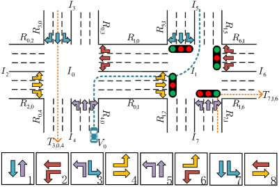
Figure 1: Visualization of two adjacent 4-arm intersections and their corresponding definitions, and 8 phases. Phase #6 is activated in $I_{1}$. We omit the turn-right traffic movements in all phases as they are always permitted in countries following right-handed driving.

Definition 4.

A vehicle route is defined as a sequence of roads $V$ with a start time $e\in\mathbb{R}$ that refers to the time when the vehicle enters the environment. Road sequence $V=\langle R^{1},R^{2},\cdots,R^{n}\rangle$, with a traffic movement $T$ from $R^{i}$ to $R^{i+1}$ for every $i\in[1,n-1]$. We assume that all vehicle routes start from/end in virtual intersections. $\mathcal{V}$ is the set of all valid vehicle routes. $V_{0}$ in Figure 1 is one example.

Definition 5.

A traffic signal phase $P_{i}$ is defined as a set of permissible traffic movements at $I_{i}$. The bottom of Figure 1 shows eight phases. $\mathcal{A}_{i}$ denotes the complete set of phases at $I_{i}$, i.e., the action space for the agent of $I_{i}$.

Problem 1.

In multi-intersection traffic signal control (M-TSC), the environment consists of intersections $\mathcal{I}$, roads $\mathcal{R}$, and vehicle routes $\mathcal{V}$. Each real intersection $I^{R}_{i}\in\mathcal{I}^{R}$ is controlled by an agent $A_{i}$. Agents perform actions between time interval $\Delta t$ based on their policies $\pi_{i}$. At time step $t$, $A_{i}$ views part of the environment $z_{i}$ as its observation, and tries to take an optimal action $a_{i}\in\mathcal{A}_{i}$ (i.e., a phase to set next) that can maximize the cumulative joint reward $r$.

As we define the M-TSC problem as a Dec-POMDP problem, we have the following RL environment settings.

True state $\boldsymbol{s}$ and partial observation $\boldsymbol{z}$. At time step $t\in\mathbb{N}$, agent $A_{i}$ has the partial observation $z_{i}^{t}\subseteq\boldsymbol{s}^{t}$, which contains the average number of vehicles $n_{x,i,y}$ following traffic movement $T_{x,i,y}\in\mathcal{T}_{i}$ and the current phase $P_{i}^{t}$.

Action $\boldsymbol{a}$. After receiving the partial observation $z_{i}^{t}$, agent $A_{i}$ chooses an action $a_{i}^{t}$ from its candidate action set $\mathcal{A}_{i}$ corresponding to a phase in next $\Delta t$ time. If the activated phase $P_{i}^{t+1}$ is different from current phase $P_{i}^{t}$, a short all-red phase will be added to avoid collision.

Joint reward $\boldsymbol{r}$. In M-TSC, we want to minimize the average travel time, which is hard to optimize directly, so some alternative metrics are chosen as immediate rewards. In this paper, we set the joint reward $r^{t}=\sum_{I_{i}\in\mathcal{I}^{R}}r_{i}^{t}$, where $r_{i}^{t}=-\overline{n^{t+1}_{x,i,y}},s.t.\ x,y\in\mathcal{I}^{N}_{i}\land T_{x,i,y}\in\mathcal{T}_{i}$ indicates the reward received by $I_{i}$, with $n_{x,i,y}$ the average vehicle number on the approaching lanes of traffic movement $T_{x,i,y}$.

4 Methods

In this section, we first propose UniComm, a new communication method, to improve the communication efficiency among agents; we then construct UniLight, a new controlling algorithm, to control signals with the help of UniComm. We use Multi-Agent Deep Q Learning Mnih et al. (2015) with double Q learning and dueling network as the basic reinforcement learning structure. Figure 2 illustrates the newly proposed model.

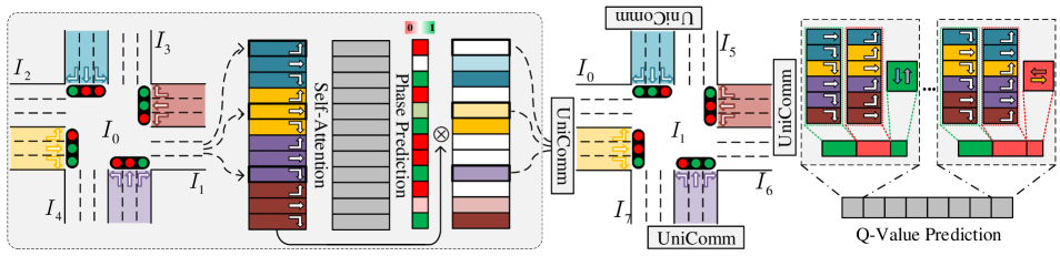
Figure 2: UniComm and UniLight structure

4.1 UniComm

The ultimate goal to enable communication between agents is to mitigate the nonstationarity caused by decentralized multi-agent learning. Sharing of more observations could help improve the stationarity, but it meanwhile suffers from the curse of dimensionality.

In existing methods, neighboring agents exchange hidden states or observations via communication. However, as mentioned above, there is no theoretical analysis on how much information is sufficient and which information is important. While with deep learning and back propagation method, we expect the network to be able to recognize information importance via well-designed structures such as attention. Unfortunately, as the training process of reinforcement learning is not as stable as that of supervised learning, the less useful or useless information might affect the convergence speed significantly. Consequently, how to enable agents to communicate effectively with their neighboring agents becomes critical. Consider intersection $I_{0}$ in Figure 1. Traffic movements such as $T_{4,0,2}$ and $T_{3,0,4}$ will not pass $R_{0,1}$, and hence their influence to $I_{1}$ is much smaller than $T_{2,0,1}$. Accordingly, we expect the information related to $T_{4,0,2}$ and $T_{3,0,4}$ to be less relevant (or even irrelevant) to $I_{1}$, as compared with information related to $T_{2,0,4}$. In other words, when $I_{0}$ communicates with $I_{1}$ and other neighboring intersections, ideally $I_{0}$ is able to pass different information to different neighbors.

We propose to share only important information with neighboring agents. To be more specific, we focus on agent $A_{1}$ on intersection $I_{1}$ which learns maximizing the cumulative reward of $r_{1}$ via reinforcement learning and evaluate the importance of certain information based on its impact on $r_{1}$.

We make two assumptions in this work. First, spillback that refers to the situation where a lane is fully occupied by vehicles and hence other vehicles cannot drive in never happens. This simplifies our study as spillback rarely happens and will disappear shortly even when it happens. Second, within action time interval $\Delta t$, no vehicle can pass though an entire road. This could be easily fulfilled, because $\Delta t$ in M-TSC is usually very short (e.g. $10s$ in our settings).

Under these assumptions, we decompose reward $r^{t}_{1}$ as follows. Recall that the reward $r^{t}_{1}$ is defined as the average of $n_{x,1,y}$ with $T_{x,1,y}\in\mathcal{T}_{1}$ being a traffic movement. As the number of traffic movements $|\mathcal{T}_{1}|$ w.r.t. intersection $I_{1}$ is a constant, for convenience, we analyze the sum of $n_{x,1,y}$, i.e. $|\mathcal{T}_{1}|r_{1}$, and $r^{t}_{1}$ can be derived by dividing the sum by $|\mathcal{T}_{1}|$.

$$|\mathcal{T}_{1}|r^{t}_{1} =\sum{n^{t+1}_{x,1,y}} x,y\in\mathcal{I}^{N}_{1}$$

$$=\sum{\left((n^{t}_{x,1,y}-m^{t}_{x,1,y})+l^{t}_{x,1,y}\right)}$$ (1)

$$=f(z^{t}_{1})+g(\boldsymbol{s}^{t})$$ (2)

In Eq. (1), we decompose $n^{t+1}_{x,1,y}$ into three parts, i.e. current vehicle number $n^{t}_{x,1,y}$, approaching vehicle number $l^{t}_{x,1,y}$, and leaving vehicle number $m^{t}_{x,1,y}$. Here, $n^{t}_{x,1,y}\in z^{t}_{1}$ can be observed directly. All leaving vehicles in $m^{t}_{x,1,y}$ are on $T_{x,1,y}$ now and can drive into next road without the consideration of spillback (based on first assumption). $P^{t}_{1}$ is derived by $\pi_{1}$, which uses partial observation $z^{t}_{1}$ as input. Accordingly, $m^{t}_{x,1,y}$ is only subject to $n^{t}_{x,1,y}$ and $P^{t}_{1}$ that both are captured by the partial observation $z^{t}_{1}$. Therefore, approaching vehicle number $l^{t}_{x,1,y}$ is the only variable affected by observations $o\notin z^{t}_{1}$. We define $f(z^{t}_{1})=\sum{(n^{t}_{x,1,y}-m^{t}_{x,1,y})}$ and $g(\boldsymbol{s}^{t})=\sum{l^{t}_{x,1,y}}$, as shown in Eq. (2).

To help and guide an agent to perform an action, agent $A_{1}$ will receive communications from other agents. Let $c^{t}_{1}$ denote the communication information received by $A_{1}$ in time step $t$. In the following, we analyze the impact of $c^{t}_{1}$ on $A_{1}$.

For observation of next phase $z^{t+1}_{1}=\{n^{t+1}_{x,1,y},P^{t+1}_{1}\}$, we have i) $n^{t+1}_{x,1,y}=n^{t}_{x,1,y}+l^{t}_{x,1,y}-m^{t}_{x,1,y}$; and ii) $P^{t+1}_{1}=\pi_{1}(z^{t}_{1},c^{t}_{1})$. As $n^{t}_{x,1,y}$ and $m^{t}_{x,1,y}$ are part of $z^{t}_{1}$, there is a function $Z_{1}$ such that $z^{t+1}_{1}=Z_{1}(z^{t}_{1},c^{t}_{1},l^{t}_{x,1,y})$. Consequently, to calculate $z^{t+1}_{1}$, the knowledge of $l^{t}_{x,1,y}$, that is not in $z^{t}_{1}$, becomes necessary. Without loss of generality, we assume $l^{t}_{x,1,y}\subseteq c^{t}_{1}$, so $z^{t+1}_{1}=Z_{1}\left(z^{t}_{1},c^{t}_{1}\right)$. In addition, $z^{t+j}_{1}$ can be represented as $Z_{j}(z^{t}_{1},c^{t}_{1},c^{t+1}_{1},\cdots,c^{t+j-1}_{1})$. Specifically, we define $Z_{0}(\cdots)=z^{t}_{1}$, regardless of the input.

We define the cumulative reward of $A_{1}$ as $R_{1}$, which can be calculated as follows:

$$R^{t}_{1} =\sum\nolimits_{j=0}^{\infty}{\gamma^{j}r^{t+j}_{1}}=\sum\nolimits_{j=0}^{\infty}{\gamma^{j}\left(f\left(z^{t+j}_{1}\right)+g\left(\boldsymbol{s}^{t+j}\right)\right)}$$

$$=\sum\nolimits_{j=0}^{\infty}{\gamma^{j}\left(f\left(Z_{j}\left(z^{t}_{1},c^{t}_{1},\cdots,c^{t+j-1}_{1}\right)\right)+g\left(\boldsymbol{s}^{t+j}\right)\right)}$$

From above equation, we set $c_{1}^{t}$ as the future values of $l$:

$$c_{1}^{t} =\left\{g\left(\boldsymbol{s}^{t}\right),g\left(\boldsymbol{s}^{t+1}\right),\cdots\right\}=\left\{\sum{l_{x,1,y}^{t}},\sum{l_{x,1,y}^{t+1}},...\right\}$$

All other variables to calculate $R_{1}^{t}$ can be derived from $c_{1}^{t}$:

$$c_{1}^{t+j}=c_{1}^{t}\backslash\{g\left(\boldsymbol{s}^{t}\right),\cdots,g\left(\boldsymbol{s}^{t+j-1}\right)\} j \in\mathbb{N}+$$

$$g\left(\boldsymbol{s}^{t+k}\right)\in c_{1}^{t} k \in\mathbb{N}$$

Hence, it is possible to derive the cumulative rewards $R_{1}^{t}$ based on future approaching vehicle numbers of traffic movements $l^{t}_{x,1,y}$s from $c_{1}^{t}$, even if other observations remain unknown. As the conclusion is universal to all existing methods on the same problem definition regardless of the network structure, we name it as UniComm. Now we convert the problem of finding the cumulative reward $R^{t}_{1}$ to how to calculate approaching vehicle numbers $l^{t}_{x,1,y}$ with current full observation $\boldsymbol{s}^{t}$. As we are not aware of exact future values, we use existing observations in $\boldsymbol{s}^{t}$ to predict $l^{t+1}_{x,1,y}$.

We first calculate approaching vehicle numbers on next interval $\Delta t$. Take intersections $I_{0},I_{1}$ and road $R_{0,1}$ for example, for traffic movement $T_{0,1,x}$ which passes intersections $I_{0}$, $I_{1}$, and $I_{x}$, approaching vehicle number $l_{0,1,x}$ depends on the traffic phase $P_{0}^{t+1}$ to be chosen by $A_{0}$. Let’s revisit the second assumption. All approaching vehicles should be on $\boldsymbol{T}_{0,1}=\{T_{y,0,1}|T_{y,0,1}\in\mathcal{T}_{0},y\in\mathcal{I}^{N}_{0}\}$, which belongs to $z^{t}_{0}$. As a result, $\boldsymbol{T}_{0,1}$ and the phase $P^{t+1}_{0}$ affect $l_{0,1,x}$ the most, even though there might be other factors.

We convert observations in $\mathcal{T}_{0}$ into hidden layers $\boldsymbol{h}_{0}$ for traffic movements by a fully-connected layer and ReLU activation function. As $P^{t+1}_{0}$ can be decomposed into the permission for every $T\in\mathcal{T}_{0}$, we use self-attention mechanism Vaswani et al. (2017) between $\boldsymbol{h}_{0}$ with Sigmoid activation function to predict the permissions $\boldsymbol{g}_{0}$ of traffic movements in next phase, which directly multiplies to $\boldsymbol{h}_{0}$. This is because for traffic movement $T_{x,0,y}\in\mathcal{T}_{0}$, if $T_{x,0,y}$ is permitted, $h_{x,0,y}$ will affect corresponding approaching vehicle numbers $l_{0,y,z}$; otherwise, it will become an all-zero vector and has no impact on $l_{0,y,z}$. Note that $R_{x,0}$ and $R_{0,y}$ might have different numbers of lanes, so we scale up the weight by the lane numbers to eliminate the effect of lane numbers. Finally, we add all corresponding weighted hidden states together and use a fully-connected layer to predict $l_{0,y,z}$.

To learn the phase prediction $P_{0}^{t+1}$, a natural method is using the action $\boldsymbol{a}_{0}$ finally taken by the current network. However, as the network is always changing, even the result phase action $\boldsymbol{a}_{0}$ corresponding to a given $\boldsymbol{s}$ is not fixed, which makes phase prediction hard to converge. To have a more stable action for prediction, we use the action $a^{r}_{0}$ stored in the replay buffer of DQN as the target, which makes the phase prediction more stable and accurate. When the stored action $a^{r}_{0}$ is selected as the target, we decompose corresponding phase $P^{r}_{0}$ into the permissions $\boldsymbol{g}^{r}_{0}$ of traffic movements, and calculate the loss between recorded real permissions $\boldsymbol{g}^{r}_{0}$ and predicted permissions $\boldsymbol{g}^{p}_{0}$ as $L_{p}=\text{BinaryCrossEntropy}(\boldsymbol{g}^{r}_{0},\boldsymbol{g}^{p}_{0})$.

For learning approaching vehicle numbers $l_{0,y,z}$ prediction, we get vehicle numbers of every traffic movement from replay buffer of DQN, and learn $l_{0,y,z}$ through recorded results $l^{r}_{0,y,z}$. As actions saved in replay buffer may be different from the current actions, when calculating volume prediction loss, different from generating UniComm, we use $\boldsymbol{g}^{r}_{0}$ instead of $\boldsymbol{g}_{0}$, i.e. $L_{v}=\text{MeanSquaredError}(\boldsymbol{g}^{r}_{0}\cdot\boldsymbol{h}_{0},l^{r}_{0,y,z})$.

Based on how $c_{1}^{t}$ is derived, we also need to predict approaching vehicle number for next several intervals, which is rather challenging. Firstly, with off-policy learning, we can’t really apply the selected action to the environment. Instead, we only learn from samples. Considering the phase prediction, while we can supervise the first phase taken by $A_{0}$, we, without interacting with the environment, don’t know the real next state $s^{\prime}\sim P(s,a)$, as the recorded $a^{r}_{0}$ may be different from $a_{0}$. The same problem applies to the prediction of $l_{0,y,z}$ too. Secondly, after multiple $\Delta t$ time intervals, the second assumption might become invalid, and it is hard to predict $l_{0,y,z}$ correctly with only $z_{0}$. As the result, we argue that as it is less useful to pass unsupervised and incorrect predictions, we only communicate with one time step prediction.

We list the pseudo code of UniComm in Algorithm 1. As the process is the same for all intersections, for simplicity, we only present the code corresponding to one intersection. The input contains current intersection observation $z$, recorded next observation $z^{r}$, the set of traffic movements $T$ of the intersection, and turning direction $d$ of traffic movements. The algorithm takes observations $o^{l}$ belong to every traffic movement, and generates embeddings $\boldsymbol{h}$ based on $o^{l}$ (lines 4-5). The permission prediction uses $\boldsymbol{h}$ with self-Attention, linear transformation and Sigmoid function, where the linear transformation is to transform an embedding to a scalar (line 6). It next calculates the phase prediction loss with recorded phase permissions using BinaryCrossEntropy Loss (line 7). Then, for every traffic movement $T_{a,x,b}\in T$, it accumulates embeddings to its corresponding outgoing lanes $\boldsymbol{h}^{p}_{x,b}$ and $\boldsymbol{h}^{r}_{x,b}$ with traffic movement embedding and permission respectively (lines 9-12). Finally, it uses linear transformation to predict the vehicle number of outgoing lanes $l$ and also volume prediction loss $L_{v}$ with MeanSquaredError Loss (lines 13-14). The algorithm outputs the estimated vehicle number $l$ for every outgoing lane of the intersection, and two prediction losses, including phase prediction loss $L_{p}$ and volume prediction loss $L_{v}$. Note that $z^{r}$ is only used to calculate $L_{p}$ and $L_{v}$.

Algorithm 1 UniComm Algorithm for an Intersection

Input: intersection index $x$, observation $z$, recorded next observation $z^{r}$, traffic movements $T$, turning direction $d$
Parameter: Traffic movement permission $\boldsymbol{g}$, traffic movement observation $o^{l}$, traffic movement embedding $\boldsymbol{h}$, out-lane prediction embedding $\boldsymbol{h}^{p}$, out-lane record embedding $\boldsymbol{h}^{r}$
Output: Estimated vehicle number $l$, phase loss $L_{p}$, volume loss $L_{v}$

1:  $(\text{Vehicle number}\ n,\text{current phase}\ P)\leftarrow z$

2:  $(\text{Recorded approaching number}\ l^{r},\text{phase}\ P^{r})\leftarrow z^{r}$

3:  $\boldsymbol{g}^{r}\leftarrow P^{r}$

4:  $o^{l}_{a,x,b}\leftarrow\{n_{a,x,b},\boldsymbol{g}_{a,x,b},d_{a,x,b}\}$

5:  $\boldsymbol{h}_{a,x,b}\leftarrow\text{Embedding}(o^{l}_{a,x,b})$

6:  $\boldsymbol{g}^{p}_{a,x,b}\leftarrow\text{Sigmoid}\left(\text{Self-Attention}(\boldsymbol{h}_{a,x,b})\right)$

7:  Let $L_{p}\leftarrow\text{BinaryCrossEntropy}(\boldsymbol{g}^{r},\boldsymbol{g}^{p})$

8:  $\boldsymbol{h}^{p}\leftarrow\boldsymbol{0},\boldsymbol{h}^{r}\leftarrow\boldsymbol{0}$

9:  for $T_{a,x,b}$ in $T$ do

10:     $\boldsymbol{h}^{p}_{x,b}\leftarrow\boldsymbol{h}^{p}_{x,b}+\boldsymbol{g}^{p}_{a,x,b}\cdot\boldsymbol{h}_{a,x,b}$

11:     $\boldsymbol{h}^{r}_{x,b}\leftarrow\boldsymbol{h}^{r}_{x,b}+\boldsymbol{g}^{r}_{a,x,b}\cdot\boldsymbol{h}_{a,x,b}$

12:  end for

13:  $l\leftarrow\text{Linear}(\boldsymbol{h}^{p})$

14:  $L_{v}\leftarrow\text{MeanSquaredError}\left(\text{Linear}(\boldsymbol{h}^{r}),l^{r}\right)$

15:  return $l$, $L_{p}$, $L_{v}$

4.2 UniLight

Although UniComm is universal, its strength might not be fully achieved by existing methods, because they do not consider the importance of exchanged information. To make better use of predicted approaching vehicle numbers and other observations, we propose UniLight to predict the Q-values.

Take prediction of intersection $I_{1}$ for example. As we predict $l_{x,1,y}$ based on traffic movements, UniLight splits average number of vehicles $n_{x,1,y}$, traffic movement permissions $\boldsymbol{g}_{1}$ and predictions $l_{x,1,y}$ into traffic movements $T_{x,1,y}$, and uses a fully-connected layer with ReLU to generate the hidden state $\boldsymbol{h}_{1}$. Next, considering one traffic phase $P$ that permits traffic movements $T_{P}$ among traffic movements $\mathcal{T}_{1}$ in $I_{1}$, we split the hidden states $\boldsymbol{h}_{1}$ into two groups $G_{1}=\{h_{p}|T_{p}\in T_{P}\}$ and $G_{2}=\{h_{x}|h_{x}\in\boldsymbol{h}_{1},T_{x}\notin T_{P}\}$, based on whether the corresponding movement is permitted by $P$ or not. As traffic movements in the same group will share the same permission in phase $P$, we consider that they can be treated equally and hence use the average of their hidden states to represent the group. Obviously, traffic movements in $G_{1}$ are more important than those in $G_{2}$, so we multiply the hidden state of $G_{1}$ with a greater weight to capture the importance. Finally, we concatenate two hidden states of groups and a number representing whether current phase is $P$ through a fully-connected layer to predict the final Q-value.

The pseudo code of UniLight is listed in Algorithm 2. Same as UniComm, we only present the code corresponding to one intersection. The input contains observation $z$, all possible phases, i.e. actions $\mathcal{A}$, traffic movements $T$ of the intersection, turning direction $d$ of traffic movements, and the estimated vehicle number $l$ for every traffic movement. It’s worth to mention that UniComm estimates $l$ for every outgoing lane, but UniLight takes $l$ for incoming lanes as inputs. Consequently, we need to arrange the estimations in a proper manner such that the output of UniComm w.r.t. an intersection become the inputs of UniLight w.r.t. an adjacent intersection. UniLight outputs Q-value estimation $Q(z,\mathcal{A})$ of current observation and all possible actions. It takes the combination of observations and incoming vehicle estimation $o^{l}$ for every traffic movement, and generates the embeddings $\boldsymbol{h}$ for them (lines 3-4). For every action $a\in\mathcal{A}$, we split traffic movement embeddings into two groups $G_{1}$ and $G_{2}$ based on whether the corresponding traffic movement is permitted by $a$ or not, i.e., $G_{1}$ consists of the embeddings of all the movements in $T$ that are permitted by $a$ and $G_{2}$ consists of the embeddings of rest of the movements in $T$ that are stopped by $a$ (lines 6-9). We use the average of embeddings to represent a group (i.e., a group embedding), and multiply the group embedding with different weights. Obviously, traffic movements in $G_{1}$ are more important than the rest traffic movements in $G_{2}$ for action $a$, so $w_{1}$ is much larger than $w_{2}$. Finally, we concatenate group embeddings with current phase $P$, and use a linear transformation to predict $Q(z,a)$ (line 10).

Algorithm 2 UniLight Algorithm for an Intersection

Input: Intersection index $x$, observation $z$, possible phases $\mathcal{A}$, traffic movements $T$, turning direction $d$, estimated vehicle number $l$
Parameter: Traffic movement permission $\boldsymbol{g}$, traffic movement observation $o_{l}$, traffic movement embedding $\boldsymbol{h}$, action phase $a$
Output: Q-values $Q(z,\mathcal{A})$

1:  $(\text{Vehicle number}\ n,\text{current phase}\ P)\leftarrow z$

2:  $\boldsymbol{g}\leftarrow P$

3:  $o^{l}_{a,x,b}\leftarrow\{n_{a,x,b},\boldsymbol{g}_{a,x,b},d_{a,x,b},l_{a,x,b}\}$

4:  $\boldsymbol{h}_{a,x,b}\leftarrow\text{Embedding}(o^{l}_{a,x,b})$

5:  for $a$ in $\mathcal{A}$ do

6:     $g^{a}\leftarrow a$

7:     $T_{a}\leftarrow\{T_{i}\in T|i:\boldsymbol{g}^{a}_{i}\text{~{}is permitted}\}$

8:     $G_{1}\leftarrow\{\boldsymbol{h}_{i}\in\boldsymbol{h}|i:T_{i}\in T_{a}\}$

9:     $G_{2}\leftarrow\boldsymbol{h}\backslash G_{1}$

10:     $Q(z,a)\leftarrow\text{Linear}\left(w_{1}\overline{G_{1}}\oplus w_{2}\overline{G_{2}}\oplus P\right)$

11:  end for

12:  return $Q(z,\mathcal{A})$

5 Experiments

In this section, we first explain the detailed experimental setup, including implementaion details, datasets used, competitors evaluated, and performance metrics employed; we then report the experimental results.

5.1 Experimental Setup

5.1.1 Implementation details

We conduct our experiments on the microscopic traffic simulator CityFlow Zhang et al. (2019). We have made some modifications to CityFlow to support the collection of structural data from the intersections and the roads. In the experiment, the action time interval $\Delta t=10s$, and the all-red phase is $5s$. We run the experiments on a cloud platform with 2 virtual Intel 8269CY CPU core and 4GB memory. We train all the methods, including newly proposed ones and the existing ones selected for comparison, with $240,000$ frames. We run all the experiments 4 times, and select the best one which will be then tested 10 times with its average performance and its standard deviation reported in our paper.

Most experiments are run on Unbuntu 20.04, PyTorch 1.7.1 with CPU only. A small part of experiments are run on GPU machines. We list the parameter settings in the following and please refer to the source codes for more detailed implementations.

For Double-Dueling DQN, we use discount factor $\gamma=0.8$ and 5-step learning. The replay buffer size is 8000. When replay buffer is fulfilled, the model is trained after every step with batch size 30, and the target network is updated every 5 steps. For $\epsilon$-greedy strategy, the initial $\epsilon=0.9$, the minimum $\epsilon=0.02$, and $\epsilon$ is decreasing linearly in the first 30% training steps.

As roads have different number of lanes and different traffic movements have various lane numbers, the average number of vehicles of one traffic movement $n$ in the observation $z$ is divided by its lane number. In UniComm, the dimension of lane embedding $\boldsymbol{h}[i]$ is 32, turning direction $d[i]$ is represented by an embedding with dimension 2, and Self-Attention used in phase prediction has one head. In UniLight, the dimension of lane embedding $h[i]$ is 32, and the weights for two groups are $w_{1}=5$ and $w_{2}=1$ respectively.

5.1.2 Datasets

We use the real-world datasets from four different cities, including Hangzhou (HZ), Jinan (JN), and Shanghai (SH) from China, and New York (NY) from USA. The HZ, JN, and NY datasets are publicly available Wei et al. (2019b), and widely used in many related studies. However, the simulation time of these three datasets is relatively short, and hence it is hard to test the performance of a signal controlling method, especially during the rush hour. We also notice that roads in these three datasets contain exactly three lanes, i.e., one lane for every turning direction. In those public datasets, the length of roads sharing the same direction is a constant (e.g., all the vertical roads share the same road length), which is different from the reality. Meanwhile, although the traffic data of public datasets is based on real traffic flow, they adopt a fixed probability distribution, as it is not possible to track all the vehicle trajectories. For example, they assume 10% of traffic flow turn left, 60% go straight, and 30% turn right to simulate vehicle trajectories, which is very unrealistic.

Motivated by the limitations of public datasets, we try to develop new datasets that can simulate the urban traffic in a more realistic manner. As taxis perform an important role in urban traffic, we utilize substantial taxi trajectories to reproduce the traffic flow for an area closer to the reality. Shanghai taxi dataset contains $11,861,593$ trajectories generated by $13,767$ taxis in the whole month of April, 2015. Directly using taxi trajectories in one day will face the data sparsity problem. To overcome data sparsity, we squash all trajectories into one day to decrease the variance and meanwhile balance the number of vehicle routes based on the traffic volume from official data to truthfully recover the traffic of one area. We choose two transportation hubs, which contain roads of different levels, i.e. roads have different number of lanes, denoted as SH₁ and SH₂ respectively. In our datasets, the two road segments belonging to the same road but having opposite directions have the same number of lanes.

Figure 3 visualizes those two hubs. The first hub SH₁ contains six intersections, which are marked by green icons. The lane numbers of the three horizontal roads are 3, 7, and 3 respectively, and the lane numbers of the two vertical roads are 3 and 4 respectively. For the second hub SH₂, it contains eight intersections. The three horizontal roads have 3, 5, and 3 lanes respectively, while all the vertical roads have 3 lanes. As stated previously, for all the roads in these two hubs, they share the same number of lanes on both directions. For example, the very wide horizontal road in SH₂ corresponds a bidirectional road in reality, and it is represented by two roads in our simulation. Those two roads have opposite directions, one from the east to the west and the other from the west to the east, but they have the same number of lanes. In reality, some small roads only contain one or two lanes, and some turning directions share one lane, e.g., in a two-lane road, the left lane can be used to turn left, and the right lane can be used to go-straight or turn right. However, lanes in CityFlow cannot share multiple turning directions as CityFlow allows each lane to have exact one turning direction. Consequently, we have to add lanes to those roads such that all the turning directions allowed in reality can be supported too in our experiments. This explains why in the second hub, the vertical road located in the middle looks wider than the other two vertical roads but it shares the same number of lanes as the other two vertical roads.

We show the statistics of all five datasets in Table 1. The average number of vehicles in 5 minutes is counted based on every single intersection in the dataset. Compared with existing datasets, the roads in our newly generated datasets SH₁ and SH₂ are more realistic. They have different number of lanes and different length, much wider time span, and the vehicle trajectories are more realistic and dynamic.

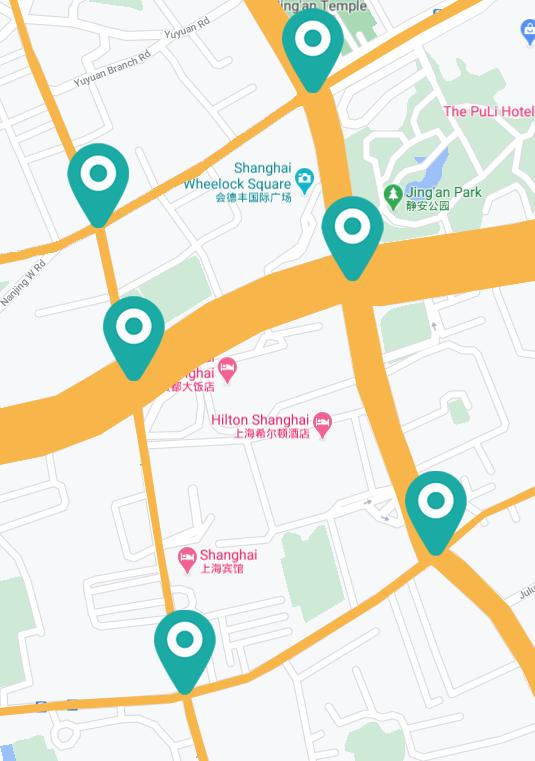
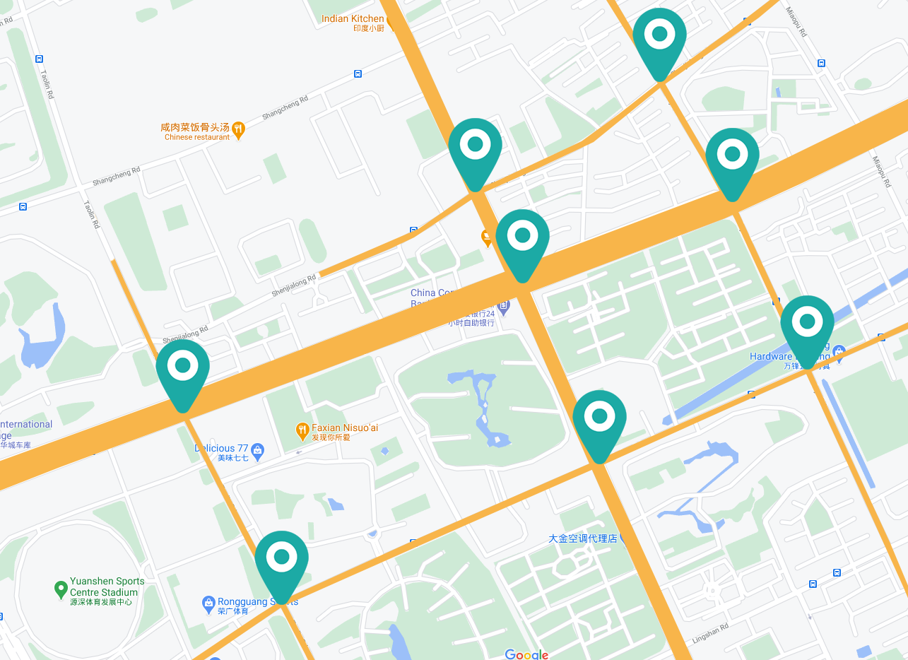
Figure 3: Real road networks of two Shanghai datasets with 6 and 8 intersections respectively. Roads with more lanes are colored with wider lines.

	HZ	JN	NY	SH1	SH2
# of Intersections	16	12	48	6	8
Road Length (metre)	600/800	400/800	100/350	62$\sim$612	102$\sim$706
# of Lanes	3	3	3	3$\sim$7	3$\sim$5
Time Span (second)	3600	3600	3600	86400	86400
# of vehicle	2983	6295	2824	22313	15741
Average # of vehicles in 5 minutes	13$\sim$21	21$\sim$57	5$\sim$6	3$\sim$76	2$\sim$52

Table 1: Datasets Statistics

5.1.3 Competitors

To evaluate the effectiveness of newly proposed UniComm and UniLight, we implement five conventional TSC methods and six representative reinforcement learning M-TSC methods as competitors, which are listed below.

(1) SOTL Cools et al. (2013), a S-TSC method based on current vehicle numbers on every traffic movement.

(2) MaxPressure Varaiya (2013), a M-TSC method that balances the vehicle numbers between two neighboring intersections.

(3) MaxBand Little et al. (1981) that maximizes the green wave time for both directions of a road.

(4) TFP-TCC Jiang et al. (2021) that predicts the traffic flow and uses traffic congestion control methods based on future traffic condition.

(5) MARLIN El-Tantawy et al. (2013) that uses Q-learning to learn joint actions for agents.

(6) MA-A2C Mnih et al. (2016), a general reinforcement learning method with actor-critic structure and multiple agents.

(7) MA-PPO Schulman et al. (2017), a popular policy based method, which improves MA-A2C with proximal policy optimization to stable the training process.

(8) PressLight Wei et al. (2019a), a reinforcement learning based method motivated by MaxPressure, which modifies the reinforcement learning RL design to use pressure as the metric.

(9) CoLight Wei et al. (2019b) that uses graph attentional network to communicate between neighboring intersections with different weights.

(10) MPLight Chen et al. (2020), a state-of-the-art M-TSC method that combines FRAP Zheng et al. (2019a) and PressLight, and is one of the state-of-the-art methods in M-TSC.

(11) AttendLight Oroojlooy et al. (2020) that uses attention and LSTM to select best actions.

5.1.4 Performance Metrics

To prove the effectiveness of our proposed methods, we have performed a comprehensive experimental study to evaluate the performance of my methods and all the competitors. Following existing studies Oroojlooy et al. (2020); Chen et al. (2020), we consider in total four different performance metrics, including average travel time, average delay, average wait time and throughput. The meanings of different metrics are listed below.

• Travel time. The travel time of a vehicle is the time it used between entering and leaving the environment.

• Delay. The delay of a vehicle is its travel time minus the expected travel time, i.e., the time used to travel when there is no other vehicles and traffic signals are always green.

• Wait time. The wait time is defined as the time a vehicle is waiting, i.e., its speed is less than a threshold. In our experiments, the threshold is set to 0.1m/s.

• Throughput. The throughput is the number of vehicles that have completed their trajectories before the simulation stops.

5.2 Evaluation Results

Datasets		JN	HZ	NY	SH1	SH2
UniLight	No Com.	335.85	324.24	186.85	2326.29	209.89
	Hidden State	330.99	323.88	180.99	1874.11	224.55
	UniComm	325.47	323.01	180.72	159.88	208.06

Table 2: Compare UniComm with hidden state in average travel time.

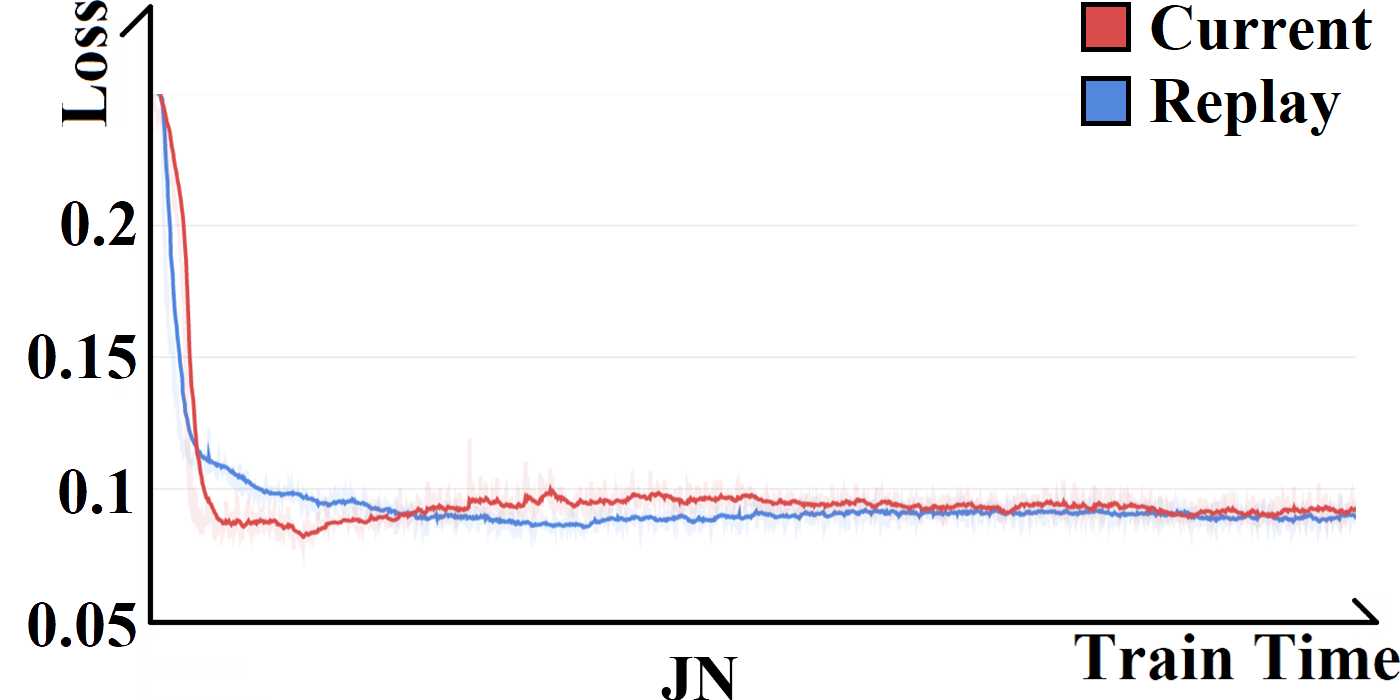
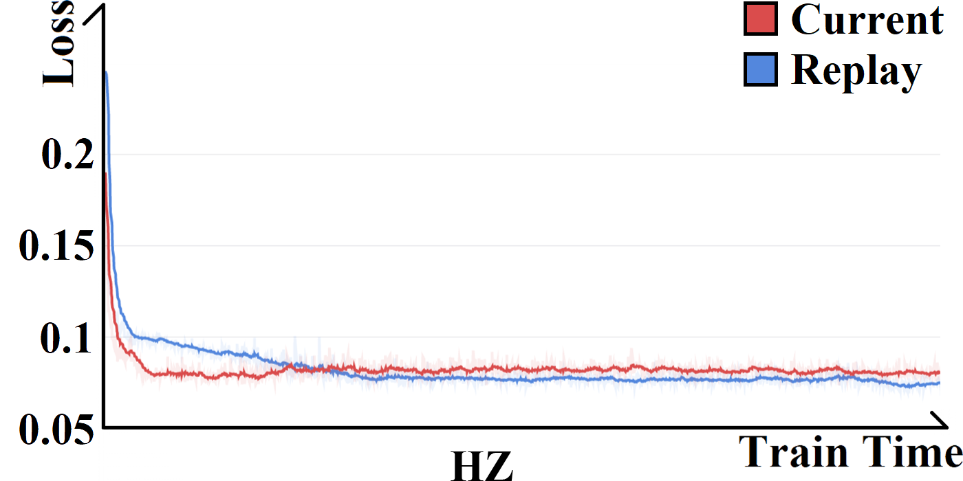
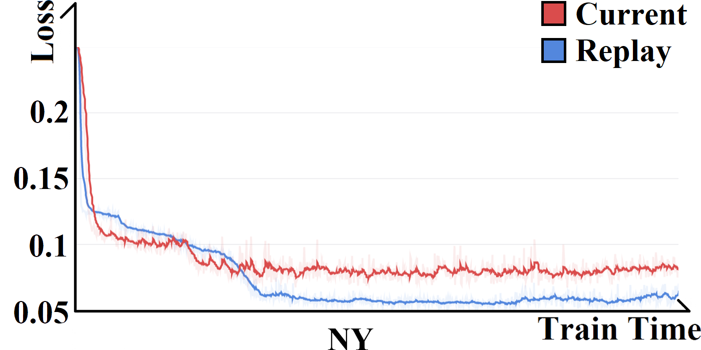
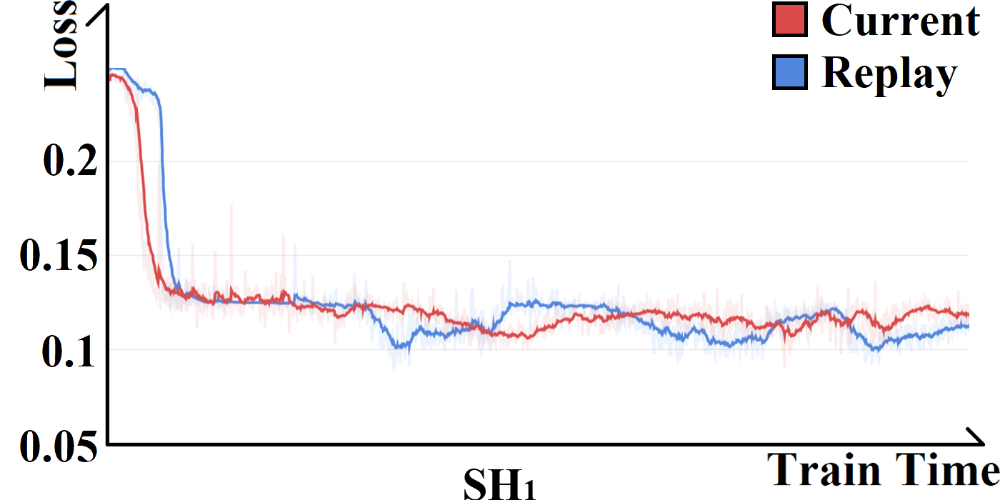
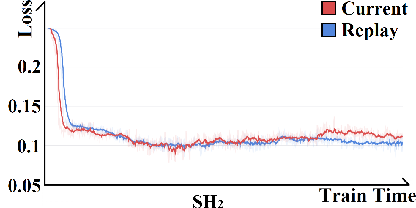
Figure 4: Phase prediction loss of different phase prediction target.

Datasets			JN	HZ	NY	SH1	SH2
Traditional	Algorithms	SOTL	420.70 $\pm$ 0.00	451.62 $\pm$ 0.00	1137.29 $\pm$ 0.00	2362.73 $\pm$ 216.82	2084.93 $\pm$ 82.83
		MaxPressure	434.75 $\pm$ 0.00	408.47 $\pm$ 0.00	243.59 $\pm$ 0.00	4843.07 $\pm$ 93.82	788.55 $\pm$ 50.06
		MaxBand	378.45 $\pm$ 2.06	458.00 $\pm$ 1.41	1038.67 $\pm$ 12.81	5675.98 $\pm$ 122.45	4501.39 $\pm$ 85.04
		TFP-TCC	362.70 $\pm$ 5.30	400.24 $\pm$ 1.42	1216.77 $\pm$ 21.27	2403.66 $\pm$ 878.66	1380.05 $\pm$ 146.18
		MARLIN	409.27 $\pm$ 0.00	388.00 $\pm$ 0.03	1274.23 $\pm$ 0.00	6623.83 $\pm$ 507.52	5373.53 $\pm$ 101.74
DRL	Algorithms	MA-A2C	355.29 $\pm$ 1.03	353.28 $\pm$ 0.82	906.71 $\pm$ 28.96	4787.83 $\pm$ 362.12	431.53 $\pm$ 41.01
		MA-PPO	460.18 $\pm$ 20.71	352.64 $\pm$ 1.18	923.82 $\pm$ 22.77	3650.83 $\pm$ 171.07	2026.71 $\pm$ 597.83
		PressLight	335.93 $\pm$ 0.00	338.41 $\pm$ 0.00	1363.31 $\pm$ 0.00	5114.78 $\pm$ 647.92	322.48 $\pm$ 3.84
		CoLight	329.67 $\pm$ 0.00	340.36 $\pm$ 0.00	244.57 $\pm$ 0.00	7861.59 $\pm$ 69.86	4438.90 $\pm$ 260.66
		MPLight	383.95 $\pm$ 0.00	334.04 $\pm$ 0.00	646.94 $\pm$ 0.00	7091.79 $\pm$ 22.97	433.92 $\pm$ 23.26
		AttendLight	361.94 $\pm$ 2.85	339.45 $\pm$ 0.82	1376.81 $\pm$ 16.41	4700.22 $\pm$ 87.50	2763.66 $\pm$ 425.19
		UniLight	335.85 $\pm$ 0.00	324.24 $\pm$ 0.00	186.85 $\pm$ 0.00	2326.29 $\pm$ 242.90	209.89 $\pm$ 21.70
With	UniComm	MA-A2C	332.80 $\pm$ 1.71	349.93 $\pm$ 1.09	834.65 $\pm$ 38.09	4018.67 $\pm$ 319.11	303.69 $\pm$ 6.13
		MA-PPO	331.96 $\pm$ 1.34	349.82 $\pm$ 1.21	847.49 $\pm$ 30.88	3806.77 $\pm$ 194.88	290.99 $\pm$ 4.23
		PressLight	317.72 $\pm$ 0.00	330.28 $\pm$ 0.00	1152.76 $\pm$ 0.00	6200.91 $\pm$ 529.39	549.56 $\pm$ 51.20
		CoLight	318.93 $\pm$ 0.00	336.66 $\pm$ 0.00	291.40 $\pm$ 0.00	7612.02 $\pm$ 271.91	1422.99 $\pm$ 633.09
		MPLight	336.29 $\pm$ 0.00	329.57 $\pm$ 0.00	193.21 $\pm$ 0.00	5095.34 $\pm$ 224.42	542.82 $\pm$ 119.56
		AttendLight	363.41 $\pm$ 3.79	330.38 $\pm$ 1.08	608.12 $\pm$ 38.59	4825.83 $\pm$ 249.90	2915.35 $\pm$ 757.95
		UniLight	325.47 $\pm$ 0.00	323.01 $\pm$ 0.00	180.72 $\pm$ 0.00	159.88 $\pm$ 1.87	208.06 $\pm$ 0.88

Table 3: Evaluation result of average travel time (seconds).

Datasets			JN	HZ	NY	SH1	SH2
Traditional	Algorithms	SOTL	260.69 $\pm$ 0.17	232.33 $\pm$ 0.04	1079.57 $\pm$ 0.00	2340.80 $\pm$ 217.95	2047.33 $\pm$ 84.18
		MaxPressure	269.30 $\pm$ 0.04	173.03 $\pm$ 0.00	120.52 $\pm$ 0.00	4827.94 $\pm$ 94.16	738.10 $\pm$ 50.68
		MaxBand	216.83 $\pm$ 2.40	237.20 $\pm$ 1.50	973.48 $\pm$ 13.43	5663.45 $\pm$ 122.96	4479.86 $\pm$ 85.46
		TFP-TCC	199.80 $\pm$ 5.11	182.46 $\pm$ 1.65	1161.35 $\pm$ 22.28	2380.09 $\pm$ 884.42	1334.86 $\pm$ 147.56
		MARLIN	247.59 $\pm$ 0.04	158.49 $\pm$ 0.08	1220.23 $\pm$ 0.00	6614.58 $\pm$ 508.83	5354.42 $\pm$ 101.87
DRL	Algorithms	MA-A2C	190.84 $\pm$ 1.29	121.30 $\pm$ 1.00	834.03 $\pm$ 30.93	4773.34 $\pm$ 363.34	378.63 $\pm$ 41.98
		MA-PPO	305.78 $\pm$ 22.30	120.53 $\pm$ 1.51	852.49 $\pm$ 24.34	3631.40 $\pm$ 171.77	1984.16 $\pm$ 603.71
		PressLight	169.30 $\pm$ 0.06	100.17 $\pm$ 0.00	1314.57 $\pm$ 0.00	5100.96 $\pm$ 649.87	267.35 $\pm$ 3.72
		CoLight	162.71 $\pm$ 0.07	98.84 $\pm$ 0.04	125.32 $\pm$ 0.00	7854.45 $\pm$ 70.14	4411.89 $\pm$ 263.23
		MPLight	218.41 $\pm$ 0.03	88.68 $\pm$ 0.00	554.87 $\pm$ 0.00	7083.68 $\pm$ 23.03	379.99 $\pm$ 23.65
		AttendLight	197.32 $\pm$ 2.62	103.16 $\pm$ 1.58	1329.94 $\pm$ 17.37	4684.92 $\pm$ 87.76	2731.29 $\pm$ 428.06
		UniLight	166.49 $\pm$ 0.01	74.93 $\pm$ 0.00	55.85 $\pm$ 0.00	2302.12 $\pm$ 244.06	153.11 $\pm$ 22.65
With	UniComm	MA-A2C	166.91 $\pm$ 1.73	117.20 $\pm$ 1.63	757.19 $\pm$ 40.58	4000.45 $\pm$ 320.40	249.05 $\pm$ 6.21
		MA-PPO	165.65 $\pm$ 1.38	116.75 $\pm$ 2.20	771.26 $\pm$ 32.83	3788.19 $\pm$ 195.69	236.43 $\pm$ 4.39
		PressLight	149.92 $\pm$ 0.05	86.35 $\pm$ 0.00	1096.51 $\pm$ 0.00	6189.67 $\pm$ 530.99	497.70 $\pm$ 52.01
		CoLight	151.00 $\pm$ 0.12	94.24 $\pm$ 0.00	176.94 $\pm$ 0.00	7605.18 $\pm$ 272.52	1379.88 $\pm$ 637.67
		MPLight	166.26 $\pm$ 0.07	81.76 $\pm$ 0.00	63.52 $\pm$ 0.00	5081.75 $\pm$ 225.04	491.35 $\pm$ 121.36
		AttendLight	197.60 $\pm$ 4.23	86.03 $\pm$ 1.76	507.25 $\pm$ 39.91	4811.16 $\pm$ 250.93	2884.94 $\pm$ 763.61
		UniLight	156.33 $\pm$ 0.04	72.63 $\pm$ 0.00	48.47 $\pm$ 0.00	119.99 $\pm$ 1.84	151.63 $\pm$ 0.93

Table 4: Evaluation result of average delay (seconds).

Datasets			JN	HZ	NY	SH1	SH2
Traditional	Algorithms	SOTL	181.40 $\pm$ 0.00	149.48 $\pm$ 0.00	1057.95 $\pm$ 0.00	2309.50 $\pm$ 220.12	1988.22 $\pm$ 87.12
		MaxPressure	197.85 $\pm$ 0.00	117.95 $\pm$ 0.00	66.44 $\pm$ 0.00	4813.49 $\pm$ 94.59	679.05 $\pm$ 53.07
		MaxBand	138.97 $\pm$ 1.95	158.44 $\pm$ 1.42	946.18 $\pm$ 14.03	5646.98 $\pm$ 124.50	4448.32 $\pm$ 86.18
		TFP-TCC	124.67 $\pm$ 4.92	105.31 $\pm$ 1.48	1142.30 $\pm$ 22.99	2346.91 $\pm$ 894.53	1268.55 $\pm$ 148.46
		MARLIN	175.82 $\pm$ 0.00	92.56 $\pm$ 0.03	1202.31 $\pm$ 0.00	6602.23 $\pm$ 510.35	5329.60 $\pm$ 104.08
DRL	Algorithms	MA-A2C	110.93 $\pm$ 1.06	54.30 $\pm$ 0.67	798.16 $\pm$ 32.82	4756.17 $\pm$ 365.55	298.59 $\pm$ 41.97
		MA-PPO	234.25 $\pm$ 25.70	53.51 $\pm$ 1.12	817.35 $\pm$ 25.36	3607.33 $\pm$ 172.69	1939.55 $\pm$ 609.96
		PressLight	94.89 $\pm$ 0.00	41.62 $\pm$ 0.00	1292.71 $\pm$ 0.00	5083.04 $\pm$ 652.50	197.60 $\pm$ 3.86
		CoLight	90.75 $\pm$ 0.00	43.16 $\pm$ 0.00	79.26 $\pm$ 0.00	7848.86 $\pm$ 70.36	4390.50 $\pm$ 263.65
		MPLight	141.80 $\pm$ 0.00	36.38 $\pm$ 0.00	520.81 $\pm$ 0.00	7075.08 $\pm$ 23.24	306.22 $\pm$ 25.09
		AttendLight	118.12 $\pm$ 2.78	42.20 $\pm$ 0.86	1313.50 $\pm$ 18.15	4660.36 $\pm$ 88.32	2669.69 $\pm$ 433.18
		UniLight	96.65 $\pm$ 0.00	27.18 $\pm$ 0.00	22.03 $\pm$ 0.00	2273.12 $\pm$ 246.13	87.10 $\pm$ 24.52
With	UniComm	MA-A2C	90.16 $\pm$ 1.55	51.30 $\pm$ 0.96	717.81 $\pm$ 42.64	3972.36 $\pm$ 323.13	170.02 $\pm$ 6.00
		MA-PPO	89.48 $\pm$ 1.26	51.49 $\pm$ 1.09	733.61 $\pm$ 34.53	3761.27 $\pm$ 197.65	160.16 $\pm$ 4.23
		PressLight	77.83 $\pm$ 0.00	32.86 $\pm$ 0.00	1065.61 $\pm$ 0.00	6173.58 $\pm$ 533.88	424.60 $\pm$ 53.66
		CoLight	79.62 $\pm$ 0.00	40.15 $\pm$ 0.00	124.21 $\pm$ 0.00	7596.31 $\pm$ 273.81	1315.25 $\pm$ 649.06
		MPLight	96.48 $\pm$ 0.00	29.62 $\pm$ 0.00	26.73 $\pm$ 0.00	5065.68 $\pm$ 226.48	438.78 $\pm$ 125.50
		AttendLight	121.75 $\pm$ 3.65	32.72 $\pm$ 1.02	435.25 $\pm$ 39.52	4787.83 $\pm$ 253.85	2833.39 $\pm$ 775.06
		UniLight	84.83 $\pm$ 0.00	25.53 $\pm$ 0.00	19.16 $\pm$ 0.00	73.46 $\pm$ 1.83	84.89 $\pm$ 1.32

Table 5: Evaluation result of average wait time (seconds).

Datasets			JN	HZ	NY	SH1	SH2
Traditional	Algorithms	SOTL	5369 $\pm$ 0	2648 $\pm$ 0	879 $\pm$ 0	11459 $\pm$ 1193	8769 $\pm$ 1042
		MaxPressure	5330 $\pm$ 0	2656 $\pm$ 0	2642 $\pm$ 0	6477 $\pm$ 216	12245 $\pm$ 383
		MaxBand	5422 $\pm$ 6	2574 $\pm$ 3	1010 $\pm$ 21	5316 $\pm$ 436	4705 $\pm$ 99
		TFP-TCC	5607 $\pm$ 17	2668 $\pm$ 5	790 $\pm$ 32	10267 $\pm$ 1458	10341 $\pm$ 24
		MARLIN	5028 $\pm$ 0	2489 $\pm$ 0	691 $\pm$ 0	2895 $\pm$ 389	3191 $\pm$ 909
DRL	Algorithms	MA-A2C	5537 $\pm$ 15	2708 $\pm$ 6	1115 $\pm$ 41	4344 $\pm$ 1701	240 $\pm$ 27
		MA-PPO	5059 $\pm$ 123	2712 $\pm$ 4	1168 $\pm$ 48	4931 $\pm$ 2131	5690 $\pm$ 743
		PressLight	5610 $\pm$ 0	2720 $\pm$ 0	492 $\pm$ 0	5066 $\pm$ 589	14162 $\pm$ 175
		CoLight	5641 $\pm$ 0	2714 $\pm$ 0	425 $\pm$ 0	1737 $\pm$ 154	4169 $\pm$ 414
		MPLight	4653 $\pm$ 0	2530 $\pm$ 0	617 $\pm$ 0	2114 $\pm$ 431	4287 $\pm$ 71
		AttendLight	5380 $\pm$ 33	2488 $\pm$ 22	411 $\pm$ 26	4470 $\pm$ 835	3972 $\pm$ 174
		UniLight	5626 $\pm$ 0	2730 $\pm$ 0	2686 $\pm$ 0	8991 $\pm$ 695	14746 $\pm$ 595
With	UniComm	MA-A2C	5662 $\pm$ 12	2711 $\pm$ 5	1192 $\pm$ 50	8091 $\pm$ 839	14433 $\pm$ 46
		MA-PPO	5662 $\pm$ 8	2711 $\pm$ 4	1249 $\pm$ 37	7440 $\pm$ 691	14453 $\pm$ 115
		PressLight	5662 $\pm$ 0	2726 $\pm$ 0	561 $\pm$ 0	2663 $\pm$ 381	7323 $\pm$ 2052
		CoLight	5675 $\pm$ 0	2715 $\pm$ 0	478 $\pm$ 0	2124 $\pm$ 401	5798 $\pm$ 413
		MPLight	5321 $\pm$ 0	2725 $\pm$ 0	721 $\pm$ 0	1285 $\pm$ 486	3854 $\pm$ 459
		AttendLight	5371 $\pm$ 10	2730 $\pm$ 3	671 $\pm$ 38	6754 $\pm$ 657	5254 $\pm$ 188
		UniLight	5654 $\pm$ 0	2739 $\pm$ 0	2688 $\pm$ 0	16928 $\pm$ 3963	14538 $\pm$ 981

Table 6: Evaluation result of average throughput (number of vehicles).

We report the results corresponding to all four metrics below, including the average values and their standard deviations, in Tables 3 to 6. Note, the standard deviation of some experiments is zero. This is because in these datasets, the environment is determined, and DQN in testing is also determined. Consequently, the results remain unchanged in all 10 tests.

5.2.1 Performance comparison without UniComm

We first focus on the results without UniComm, i.e., all competitors communicate in their original way, and UniLight runs without any communication. The numbers in bold indicate the best performance. We observe that RL based methods achieve better results than traditional methods in public datasets. However, in a complicated environment like SH₁, agents may fail to learn a valid policy, and accordingly RL based methods might perform much worse than the traditional methods.

UniLight performs the best in almost all datasets, and it demonstrates significant advantages in complicated environments. It improves the average performance by 8.2% in three public datasets and 35.6% in more complicated environments like SH₁/SH₂. We believe the improvement brought by UniLight is mainly contributed by the following two features of UniLight. Firstly, UniLight divides the input state into traffic movements and uses the same model layer to generate corresponding hidden states for different traffic movements. As the layer is shared by all traffic movements regardless of traffic phases selected, the model parameters can be trained more efficiently. For example, the intersection shown in Figure 1 has 12 traffic movements. For every input state, the model layer is actually trained 12 times. Secondly, to predict Q-value of traffic phase $P$, we split hidden states of traffic movements into two groups based on their permissions and aggregate hidden states from same groups, so the model layer to predict Q-value can be used by different phases. This again implies that the layer is trained more times so it’s able to learn better model weights.

JN dataset is the only exception, where CoLight and PressLight perform slightly better than UniLight. This is because many roads in JN dataset share the same number of approaching vehicles, which makes the controlling easier, and all methods perform similarly.

5.2.2 The Impact of UniComm

As UniComm is universal for existing methods, we apply UniComm to the six representative RL based methods and re-evaluate their performance, with results listed in the bottom portion of Tables 3 to 6. We observe that UniLight again achieves the best performance consistently. In addition, almost all RL based methods (including UniLight) are able to achieve a better performance with UniComm. This is because UniComm predicts the approaching vehicle number on $R_{i,j}$ mainly by the hidden states of traffic movements covering $R_{i,j}$. Consequently, $A_{i}$ is able to produce predictions for neighboring $A_{j}$ based on more important/relevant information. As a result, neighbors will receive customized results, which allow them to utilize the information in a more effective manner. In addition, agents only share predictions with their neighbors so the communication information and the observation dimension remain small. This allows existing RL based methods to outperform their original versions whose communications are mainly based on hidden states. Some original methods perform worse with UniComm in certain experiments, e.g. PressLight in SH₁. This is because these methods have unstable performance on some datasets with very large variance, which make the results unstable. Despite of a small number of outliers, UniComm makes consistent boost on all existing methods.

5.2.3 Phase Prediction Target Evaluation

As mentioned previously, instead of directly using current phase action to calculate phase prediction loss $L_{p}$, we use actions stored in replay buffer. To evaluate its effectiveness, we plot the curve of $L_{p}$ in Figure 4. Current and Replay refer to the use of the action taken by the current network and that stored in the replay buffer respectively when calculating $L_{p}$. The curve represents the volume prediction loss, i.e. the prediction accuracy during the training process. We can observe that when using stored actions as the target, the loss becomes smaller, i.e., it has learned better phase predictions. The convergence speed of phase prediction loss with stored actions is slower at the beginning of the training. This is because to perform more exploration, most actions are random at the beginning, which is hard to predict.

5.2.4 UniComm vs. Hidden States

To further evaluate the effectiveness of UniComm from a different angle, we introduce another version of UniLight that uses a 32-dimension hidden state for communication, the same as Wei et al. (2019b). In total, there are three different versions of UniLight evaluated, i.e., No Com., Hidden State, and UniComm. As the names suggest, No Com. refers to the version without sharing any information as there is no communication between agents; Hidden State refers to the version sharing 32-dimension hidden state; and UniComm refers to the version that implements UniComm. The average travel time of all the vehicles under these three variants of UniLight is listed in Table 2. Note, Hidden State shares the most amount of information and is able to improve the performance, as compared with version of No Com.. Unfortunately, the amount of information shared is not proportional to the performance improvement it can achieve. For example, UniLight with UniComm performs better than the version with Hidden State, although it shares less amount of information. This further verifies our argument that the content and the importance of the shared information is much more important than the amount.

6 Conclusion

In this paper, we propose a novel communication form UniComm for decentralized multi-agent learning based M-TSC problem. It enables each agent to share the prediction of approaching vehicles with its neighbors via communication. We also design UniLight to predict Q-value based on UniComm. Experimental results demonstrate that UniComm is universal for existing M-TSC methods, and UniLight outperforms existing methods in both simple and complex environments.

References

- Arel et al. [2010] Itamar Arel, Cong Liu, Tom Urbanik, and Airton G Kohls. Reinforcement learning-based multi-agent system for network traffic signal control. IET Intelligent Transport Systems, 4(2):128–135, 2010.
- Ault et al. [2020] James Ault, Josiah P. Hanna, and Guni Sharon. Learning an interpretable traffic signal control policy. In AAMAS 2020, pages 88–96, 2020.
- Bishop [2006] Christopher M Bishop. Pattern recognition and machine learning. springer, 2006.
- Chen et al. [2020] Chacha Chen, Hua Wei, Nan Xu, Guanjie Zheng, Ming Yang, Yuanhao Xiong, Kai Xu, and Zhenhui Li. Toward a thousand lights: Decentralized deep reinforcement learning for large-scale traffic signal control. In AAAI 2020, pages 3414–3421, 2020.
- Cools et al. [2013] Seung-Bae Cools, Carlos Gershenson, and Bart D’Hooghe. Self-Organizing Traffic Lights: A Realistic Simulation, pages 45–55. Springer London, London, 2013.
- El-Tantawy et al. [2013] Samah El-Tantawy, Baher Abdulhai, and Hossam Abdelgawad. Multiagent reinforcement learning for integrated network of adaptive traffic signal controllers (marlin-atsc): methodology and large-scale application on downtown toronto. IEEE Transactions on Intelligent Transportation Systems, 14(3):1140–1150, 2013.
- Haarnoja et al. [2018] Tuomas Haarnoja, Aurick Zhou, Pieter Abbeel, and Sergey Levine. Soft actor-critic: Off-policy maximum entropy deep reinforcement learning with a stochastic actor. In ICML 2018, pages 1856–1865, 2018.
- Jiang et al. [2021] Chun-Yao Jiang, Xiao-Min Hu, and Wei-Neng Chen. An urban traffic signal control system based on traffic flow prediction. In ICACI 2021, pages 259–265. IEEE, 2021.
- Little et al. [1981] John DC Little, Mark D Kelson, and Nathan H Gartner. Maxband: A versatile program for setting signals on arteries and triangular networks. 1981.
- Mnih et al. [2015] Volodymyr Mnih, Koray Kavukcuoglu, David Silver, Andrei A Rusu, Joel Veness, Marc G Bellemare, Alex Graves, Martin Riedmiller, Andreas K Fidjeland, Georg Ostrovski, et al. Human-level control through deep reinforcement learning. nature, 518(7540):529–533, 2015.
- Mnih et al. [2016] Volodymyr Mnih, Adrià Puigdomènech Badia, Mehdi Mirza, Alex Graves, Timothy P. Lillicrap, Tim Harley, David Silver, and Koray Kavukcuoglu. Asynchronous methods for deep reinforcement learning. In ICML 2016, pages 1928–1937, 2016.
- Nishi et al. [2018] Tomoki Nishi, Keisuke Otaki, Keiichiro Hayakawa, and Takayoshi Yoshimura. Traffic signal control based on reinforcement learning with graph convolutional neural nets. In ITSC 2018, pages 877–883, 2018.
- Nowé et al. [2012] Ann Nowé, Peter Vrancx, and Yann-Michaël De Hauwere. Game theory and multi-agent reinforcement learning. Springer, 2012.
- Oliehoek et al. [2016] Frans A Oliehoek, Christopher Amato, et al. A concise introduction to decentralized POMDPs, volume 1. Springer, 2016.
- Oroojlooy et al. [2020] Afshin Oroojlooy, MohammadReza Nazari, Davood Hajinezhad, and Jorge Silva. Attendlight: Universal attention-based reinforcement learning model for traffic signal control. In NeurIPS 2020, 2020.
- Schulman et al. [2017] John Schulman, Filip Wolski, Prafulla Dhariwal, Alec Radford, and Oleg Klimov. Proximal policy optimization algorithms. CoRR, abs/1707.06347, 2017.
- van Hasselt et al. [2016] Hado van Hasselt, Arthur Guez, and David Silver. Deep reinforcement learning with double q-learning. In Dale Schuurmans and Michael P. Wellman, editors, AAAI 2016, pages 2094–2100, 2016.
- Varaiya [2013] Pravin Varaiya. Max pressure control of a network of signalized intersections. Transportation Research Part C: Emerging Technologies, 36:177–195, 2013.
- Vaswani et al. [2017] Ashish Vaswani, Noam Shazeer, Niki Parmar, Jakob Uszkoreit, Llion Jones, Aidan N. Gomez, Lukasz Kaiser, and Illia Polosukhin. Attention is all you need. In NeurIPS 2017, pages 5998–6008, 2017.
- Wei et al. [2019a] Hua Wei, Chacha Chen, Guanjie Zheng, Kan Wu, Vikash Gayah, Kai Xu, and Zhenhui Li. Presslight: Learning max pressure control to coordinate traffic signals in arterial network. In SIGKDD 2019, pages 1290–1298, 2019.
- Wei et al. [2019b] Hua Wei, Nan Xu, Huichu Zhang, Guanjie Zheng, Xinshi Zang, Chacha Chen, Weinan Zhang, Yanmin Zhu, Kai Xu, and Zhenhui Li. Colight: Learning network-level cooperation for traffic signal control. In CIKM 2019, pages 1913–1922, 2019.
- Yu et al. [2020] Zhengxu Yu, Shuxian Liang, Long Wei, Zhongming Jin, Jianqiang Huang, Deng Cai, Xiaofei He, and Xian-Sheng Hua. Macar: Urban traffic light control via active multi-agent communication and action rectification. In IJCAI 2020, pages 2491–2497, 7 2020.
- Zang et al. [2020] Xinshi Zang, Huaxiu Yao, Guanjie Zheng, Nan Xu, Kai Xu, and Zhenhui Li. Metalight: Value-based meta-reinforcement learning for traffic signal control. In AAAI 2020, pages 1153–1160, 2020.
- Zhang et al. [2019] Huichu Zhang, Siyuan Feng, Chang Liu, Yaoyao Ding, Yichen Zhu, Zihan Zhou, Weinan Zhang, Yong Yu, Haiming Jin, and Zhenhui Li. Cityflow: A multi-agent reinforcement learning environment for large scale city traffic scenario. In WWW 2019, pages 3620–3624, 2019.
- Zheng et al. [2019a] Guanjie Zheng, Yuanhao Xiong, Xinshi Zang, Jie Feng, Hua Wei, Huichu Zhang, Yong Li, Kai Xu, and Zhenhui Li. Learning phase competition for traffic signal control. In CIKM 2019, pages 1963–1972, 2019.
- Zheng et al. [2019b] Guanjie Zheng, Xinshi Zang, Nan Xu, Hua Wei, Zhengyao Yu, Vikash V. Gayah, Kai Xu, and Zhenhui Li. Diagnosing reinforcement learning for traffic signal control. CoRR, abs/1905.04716, 2019.