Coefficient Mutation in the Gene-pool Optimal Mixing Evolutionary Algorithm for Symbolic Regression

Abstract.

Currently, the genetic programming version of the gene-pool optimal mixing evolutionary algorithm (GP-GOMEA) is among the top-performing algorithms for symbolic regression (SR). A key strength of GP-GOMEA is its way of performing variation, which dynamically adapts to the emergence of patterns in the population. However, GP-GOMEA lacks a mechanism to optimize coefficients. In this paper, we study how fairly simple approaches for optimizing coefficients can be integrated into GP-GOMEA. In particular, we considered two variants of Gaussian coefficient mutation. We performed experiments using different settings on 23 benchmark problems, and used machine learning to estimate what aspects of coefficient mutation matter most. We find that the most important aspect is that the number of coefficient mutation attempts needs to be commensurate with the number of mixing operations that GP-GOMEA performs. We applied GP-GOMEA with the best-performing coefficient mutation approach to the data sets of SRBench, a large SR benchmark, for which a ground-truth underlying equation is known. We find that coefficient mutation can help re-discovering the underlying equation by a substantial amount, but only when no noise is added to the target variable. In the presence of noise, GP-GOMEA with coefficient mutation discovers alternative but similarly-accurate equations.

1. Introduction

Symbolic regression (SR) is the task of discovering a governing mathematical equation that underlies the given data (Koza, 1994). Algorithms implementing SR can be of wildly different nature, including exhaustive or greedy search strategies (McConaghy, 2011; Kammerer et al., 2020; de França, 2018; Rivero et al., 2022), genetic programming (GP) and other evolutionary approaches (Koza, 1994; Schmidt and Lipson, 2009; Kantor et al., 2021), deep neural networks (Petersen et al., 2019; Biggio et al., 2021; d’Ascoli et al., 2022), as well as hybrids (Cranmer et al., 2020) and pipelines (Udrescu and Tegmark, 2020).

A recent, large benchmark study called SRBench has demonstrated that GP-based algorithms are among the best approaches for tackling SR (La Cava et al., 2021). Generally, GP works by initializing a random population of candidate solutions and improving this population in an iterative fashion, by means of component recombination between parent solutions, mutation, and stochastic survival of the fittest (Koza, 1994). At the time of writing, one of the top-performing algorithms in SRBench is the GP version of the gene-pool optimal mixing evolutionary algorithm (GP-GOMEA) (Virgolin et al., 2017, 2021), which strikes a good balance in terms of delivering small but accurate solutions. In fact, obtaining small, simple solutions is important in SR to enhance the chance that these solutions will be interpretable (Virgolin et al., 2022) (else, one may as well use uninterpretable methods such as deep neural networks for non-linear regression (Kadra et al., 2021)).

A key strength behind the performance of GP-GOMEA is its particular form of variation, which is not completely at random as is the case, e.g., for classic subtree crossover (Koza, 1994). Every generation, GP-GOMEA infers a statistical model of promising crossover masks based on the emergence of component patterns, and then uses the crossover masks to perform mixing operations. While GP-GOMEA has been shown capable of performing particularly well, there is no mechanism included that is aimed at optimizing coefficients (i.e., constants) that appear in the solutions. In fact, coefficients are sampled at random during initialization, and only swapped among solutions during variation. This means that, for GP-GOMEA to obtain a certain coefficient that has not been sampled at initialization (e.g., $2.3$), a pattern of components need to be opportunely assembled (e.g., $1.2\times 2.0-0.1$). Hence, reaching a specific coefficient with high numerical precision is unlikely, and even obtaining a coarse approximation might be inefficient.

In this paper, we consider simple evolution-based approaches for coefficient optimization in GP, and evaluate different ways of integrating them in GP-GOMEA. In particular, we consider two types of Gaussian mutations, one inspired from temperature decay in simulated annealing (Van Laarhoven and Aarts, 1987) and one from evolution strategies (Beyer and Schwefel, 2002), and assess at what point during GP-GOMEA such mutations should be applied, with what probability, and for how many attempts. We opted for random coefficient mutation instead of gradient descent, which is leveraged in many machine learning algorithms (Bottou, 2010), because the former does not require differentiability and is therefore more generally applicable. Moreover, it represents a reasonable starting point for a first study on including coefficient optimization in GP-GOMEA, and can be used as a baseline for comparing more involved approaches in the future (e.g., the Levenberg-Marquardt algorithm (Moré, 1978), which is adopted within GP in (Kommenda et al., 2020)). We remark that findings on coefficient optimization in classic GP (such as in (Kommenda et al., 2020; Dick et al., 2020)) do not necessarily apply to GP-GOMEA because variation in GP-GOMEA is very different than in classic GP (see Sec. 2.2).

The remainder of this paper is organized as follows. In Sec. 2, we formalize the problem setting of SR, provide a salient background on GP-GOMEA, and report on related work. In Sec. 3, we introduce the coefficient mutation approaches considered here. Sec. 4 describes the experimental setup. In Sec. 5 we perform an experiment on 23 benchmark data sets taken from those considered in (Oliveira et al., 2018), aimed at understanding what coefficient mutation approach is most promising in GP-GOMEA. Then in Sec. 6, we apply our findings to the data sets of SRBench for which the data-generating equation is known (so-called Feynman and Strogatz data sets), to assess whether coefficient mutation can help GP-GOMEA to recover the true underlying equation. Sec. 7 contains a discussion on the overall findings of this paper and Sec. 8 concludes it.

2. Background

2.1. Symbolic regression

In SR, we are given a data set $\mathcal{D}=\{\left(\mathbf{x}_{i},y_{i}\right)\}^{n}_{i=1}$ where $i$ is the index of an observation, $\mathbf{x}_{i}=\left(x^{(1)}_{i},x^{(2)}_{i},\dots x^{(d)}_{i}\right)^{\top}\in\mathbb{R}^{d}$ is a vector of $d$ feature values, and $y_{i}\in\mathbb{R}$ is the target variable (also called dependent variable or label). We are tasked with finding a function $f$ from a family of functions $\Omega$ such that, $\forall i,f(\mathbf{x}_{i})\approx y_{i}$.

The difference between SR and traditional regression lies in $\Omega$. In the latter, we choose $\Omega$ to contain functions that can only be different in terms of numerical coefficients $\Theta=(\theta_{1},\dots,\theta_{k})^{\top}\in\mathbb{R}^{k}$. For example for linear regression, $k=d+1$ and $\Omega$ contains all functions of the form $f_{\Theta}(\mathbf{x}):=\theta_{1}x^{(1)}+\theta_{2}x^{(2)}+\dots+\theta_{d}x^{(d)}+\theta_{d+1}$.

In SR, besides $\Theta$, $\Omega$ is defined in terms of a set of atomic functions, hereafter denoted by $\mathcal{F}$. For example, a possible choice of $\mathcal{F}$ is $\{+,-,\times,\div,\sin,\cos,\exp,\log\}$. A function in $\Omega$ is then any function that can be obtained by composition of the atomic functions in $\mathcal{F}$, together with the features and arbitrary numerical coefficients. For example for the choice of $\mathcal{F}$ made above, $f_{a}\left(x^{(1)},x^{(2)}\right):=x^{(1)}\times\sin x^{(2)}-4$ belongs to $\Omega$, while $f_{b}\left(x^{(1)}\right):=\sqrt{x^{(1)}}$ does not.

2.2. GP-GOMEA

GP-GOMEA operates as many other GP algorithms, i.e., by iterative improvement of a population of candidate solutions which are typically initially randomly generated. However, GP-GOMEA also has some notable differences. The overall workings of GP-GOMEA are displayed in Alg. 1, while a detailed description is given in the following sections.

Algorithm 1 Overall workings of GP-GOMEA

1:$\mathcal{P}\leftarrow\text{InitializePopulation}()$ # See Sec. 2.2.1

2:while $\text{BudgetLeft}()$ do

3:     $\text{FOS}\leftarrow\text{BuildFOS}(\mathcal{P})$ # See Sec. 2.2.2

4:     $\mathcal{O}\leftarrow\emptyset$

5:     for $p_{i}\in\mathcal{P}$ do

6:         $o_{i}\leftarrow\text{GOM}(p_{i},\text{FOS},\mathcal{P})$ # See Sec. 2.2.3

7:         $\mathcal{O}\leftarrow\mathcal{O}\cup\{o_{i}\}$

8:     end for

9:     $\mathcal{P}\leftarrow\mathcal{O}$

10:end while

2.2.1. Representation

Like classic GP (Koza, 1994), GP-GOMEA performs SR by encoding the evolving equations with trees. Internal nodes implement the atomic functions, while leaf nodes implement features or coefficients (constants). However, in GP-GOMEA all trees adhere to a same template; see Fig. 1. Given a maximal depth, the template consists of a full $m$-ary tree, where $m$ is the maximal arity (i.e., number of input arguments) among the atomic functions in $\mathcal{F}$. Not all nodes in the template are always active , i.e., there can be introns. Namely, for a node implementing a function of arity $a<m$, only the left-most $a$ child nodes are used as input arguments (features and coefficients are considered to have null arity).

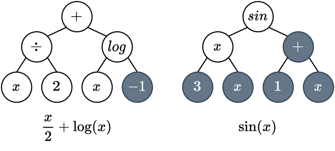
Figure 1. Two examples of the tree-based encoding of GP-GOMEA for maximal depth $2$ and maximal arity $2$. Gray nodes are introns.

2.2.2. Family of subsets

The reason why GP-GOMEA enforces trees to fit a template is to allow a positional recombination akin to genetic algorithms, which naturally fits the implementation of a statistical model representing promising crossover masks. Let $\ell$ be the maximum number of nodes in the template tree used in GP-GOMEA. Then, in an fixed tree parsing order, any node position is uniquely identified with an index in $\{1,2,\dots,\ell\}$. For example using pre-order parsing, index $1$ identifies the root node, index $2$ the left-most child of the root node, and $\ell$ the right-most leaf. We can now define the family of subsets (FOS), which is a set of sets (called subsets) which, in turn, contain node indices. For example, a possible FOS is $\{\{1\},\{3\},\{1,2\},\{1,2,3\}\}$, with $\{1,2\}$ being one of the subsets of this FOS. GP-GOMEA uses the FOS to perform mixing operations, using each subset as a crossover mask. For example the subset $\{3\}$ prescribes to generate an offspring by changing the 3rd node, while $\{1,2\}$ prescribes to change the first and second node, importantly, at the same time.

Now, under the hypothesis that encoding positions that exhibit strong inter-dependencies should be recombined jointly (i.e., as building blocks), the default FOS of GP-GOMEA is the linkage tree (LT) (Thierens, 2010). The LT is built by (1) measuring the mutual information between pairs of node positions (each node position is seen as a random variable, and the population is seen as a sample from this random variable), and (2) approximating higher-order interaction levels by means of hierarchical clustering. This results in a tree-like structure, hence the name “LT” (not to be confused with the trees used to represent solutions). Implementation details, including a normalization step to account for the lack of uniformity of the distribution in the initial population of GP, are reported in (Virgolin et al., 2021).

2.2.3. Gene-pool optimal mixing

The gene-pool optimal mixing (GOM) variation operator is used to generate an offspring from a parent solution. The pseudo-code of GOM is presented in Alg. 2; the strategies of coefficient mutation included in the pseudo-code are described later, in Sec. 3.2. GOM is applied to every population member. First, a clone of the solution is created. Then, GOM performs as many steps, or mixing attempts, as the number of subsets in the FOS to improve this clone. For each subset of the FOS (considered in random order), a GOM step consists of (1) considering the nodes identified by the subset (e.g., $\{1,4,5\}$ identifies the first, fourth, and fifth node, according to the chosen tree parsing order), (2) picking a random member of the population to act as donor, and (3) replacing the nodes identified by the subset in the offspring with the corresponding nodes from the donor. If this mixing attempt leads to equal or better fitness, the change is kept, else, the change is rolled back (see Alg. 3). For efficiency, the fitness is evaluated only when the mixing attempt is meaningful: evaluation is not performed when the nodes copied from the donor represent the same functions as those already present in the offspring, or the nodes copied from the donor end up in intron positions and thus do not influence the computations carried out by the tree (or a combination of the two).

Note that since the LT contains $2\ell-2$ subsets (details in (Virgolin et al., 2021)) and a fitness evaluation is performed after every meaningful recombination attempt, GP-GOMEA typically performs many more fitness evaluations per generation than classic GP (where each solution is evaluated once). As mentioned in the introduction, this different way of performing recombination calls for an assessment of how coefficient optimization can best be integrated in GP-GOMEA.

Algorithm 2 GOM, including the different strategies we investigated for when to apply coefficient mutation (in green)

1:function GOM($p,\text{FOS},\mathcal{P}$)

2:     $o\leftarrow\text{Clone}(p)$ # Clones components and also fitness

3:     for $S\in\text{FOS}$ do # Subsets considered in random order

4:         # Beginning of a GOM step

5:         $d\leftarrow\text{SampleRandomDonor}(\mathcal{P})$

6:         $o^{\prime}\leftarrow\text{InheritNodesBySubset}(o,d,S)$

7:         # Strategy 4 is applied within a GOM step

8:         if Strategy 4 then

9:              $o^{\prime}\leftarrow\text{CoefficientMutationToNodesBySubset}(o^{\prime},S)$

10:         end if

11:         $o\leftarrow\text{AssessChangesAndReturnBest}(o^{\prime},o)$ # Alg. 3

12:         # End of a GOM step

13:         # Strategy 3 is applied in between GOM steps

14:         if Strategy 3 then

15:              $o^{\prime}\leftarrow\text{CoefficientMutation}(o)$

16:              $o\leftarrow\text{AssessChangesAndReturnBest}(o^{\prime},o)$ # Alg. 3

17:         end if

18:     end for

19:     # Strategies 1 and 2 are applied after GOM has been completed

20:     if Strategy1 or Strategy2 then

21:         $k\leftarrow 1\textbf{ if }\text{Strategy1},\textbf{ else }|\text{FOS}|$

22:         for $i\in 1,\dots,k$ do

23:              $o^{\prime}\leftarrow\text{CoefficientMutation}(o)$

24:              $o\leftarrow\text{AssessChangesAndReturnBest}(o^{\prime},o)$ # Alg. 3

25:         end for

26:     end if

27:     return $o$

28:end function

Algorithm 3 Auxiliary function used to decide whether changes should be kept or discarded

1:function AssessChangesAndReturnBest($o^{\prime},o$)

2:     if $\text{NoMeaningfulChange}(o,o^{\prime})$ then # E.g., introns

3:         return $o^{\prime}$ # Changes led to same fitness

4:     end if

5:     $\text{Fitness}(o^{\prime})\leftarrow\text{EvaluateFitness}(o^{\prime})$ # Evaluation needed

6:     if $\text{Fitness}(o^{\prime})\geq\text{Fitness}(o)$ then # Assume maximization

7:         return $o^{\prime}$ # Changes led to equal or better fitness

8:     end if

9:     return $o$ # Changes led to worse fitness

10:end function

2.3. Related work

A number of works has considered coefficient optimization in GP. An early approach is (Howard and D’Angelo, 1995), where a genetic algorithm is integrated within GP, to optimize the coefficients. Because of its efficiency, many works use differentiable atomic functions and (variants of) gradient-descent. One of such works is (Topchy and Punch, 2001), where gradient descent is integrated in tree-based GP, and tested in a Baldwinian or Lamarckian fashion. In (Kommenda et al., 2020), instead of gradient descent, the Levenberg-Marquardt algorithm is adopted. (Zhang and Smart, 2005) and (Izzo et al., 2017) use gradient descent to optimize multiplicative coefficients placed at the edges connecting nodes, respectively in tree-based and Cartesian genetic programming (Miller and Smith, 2006). A similar formulation is considered in (Trujillo et al., 2014), using a trust region method to optimize the coefficients. Lastly, (La Cava et al., 2018) uses a differentiable multi-tree representation where gradient descent optimizes inter- and intra-tree coefficients. Several works have proposed to optimize coefficients using (different types of) coefficient mutation, typically in tree-based GP (Evett and Fernandez, 1998; Babovic and Keijzer, 2000; Langdon and Nordin, 2000; Hein et al., 2018). The hybrid neural-evolutionary approach in (Cranmer et al., 2020) includes coefficient optimization with both dedicated mutations and the Nelder-Mead algorithm (Nelder and Mead, 1965). In this work we consider two versions of coefficient mutation in GP-GOMEA; to the best of our knowledge, coefficient optimization has not been attempted before in GP-GOMEA.

3. Coefficient mutation

We use the traditional representation of numerical coefficients by which they are implemented as leaf nodes returning a constant output. These constant nodes are generated during population initialization, alongside leaf nodes that represent problem variables (in the case of SR, features of the data set). We consider the use of ephemeral random constants, i.e., constant nodes whose value is decided at the moment of their instantiation, according to the chosen distribution (Poli et al., 2008). Traditionally, GP-GOMEA does not include subtree or one-point mutation, thus random initialization is solely responsible for what coefficients will be available for the entire evolutionary process (however, a version of GOMEA for grammatical evolution includes mutation (Medvet et al., 2018)).

We consider two coefficient mutation approaches that update a current constant value $c$ with the rule:

(1) $$c^{\prime}=\delta(c,\mathcal{H}),$$

where $\mathcal{H}$ is a set of $k$ hyper-parameters and $\delta:\mathbb{R}^{1+k}\rightarrow\mathbb{R}$ is the update rule. We remark that having the update rule depend on $c$ means that the new value of the coefficient will depend on the previous value, as opposed to be generated irrespective of it, e.g., as done when replacing a constant leaf node with another one in one-point mutation.

In the next sections, we describe the two ways of implementing $\delta$ and the strategies to integrate coefficient mutation in GP-GOMEA that we considered.

3.1. Coefficient mutation types (how to optimize)

3.1.1. Evolution strategy-like

The first approach we consider is inspired by the self-adaptation mechanism in evolution strategies (ES) (Beyer and Schwefel, 2002). Each constant node contains a meta-parameter $\sigma$ that is specific to that node, and is initialized with:

(2) $$\sigma=\max\left(\exp(\mathcal{N}(0,\gamma^{2})),\epsilon\right),$$

with $\mathcal{N}(0,1)$ being the normal distribution with null mean and unit variance, and $\gamma$ and $\epsilon$ being real-valued hyper-parameters common to all constant nodes. In this paper, we fix $\gamma=0.1$ and $\epsilon=10^{-16}$.

The update rule for the coefficient the constant node represents is then:

(3) $$c^{\prime}=\mathcal{N}(c,\sigma^{2}),$$

and, importantly, when the update is triggered, then also $\sigma$ is updated, with:

(4) $$\sigma^{\prime}=\max\left(\sigma\exp(\mathcal{N}(0,\gamma^{2})),\epsilon\right).$$

The intuition is that constant nodes will implicitly evolve the update parameter $\sigma$ to become appropriate, e.g., for two nodes with the right coefficient $c$, the node with smaller $\sigma$ will be more likely to lead to a good fitness and survive. We call this approach ES-like.

3.1.2. Temperature-based

The second approach we consider is the one used in (Hein et al., 2018), i.e.,

(5) $$c^{\prime}=\mathcal{N}(c,(c\tau)^{2}),$$

where $\tau\in\mathbb{R}$ is a hyper-parameter, which we call temperature, common to all constant nodes. Note that with this temperature-based approach, coefficients with larger magnitude will necessarily have larger mutations than coefficients with smaller magnitude.

While the ES-like approach has an adaptive way of sampling thanks to $\sigma$ being implicitly evolved, the same is not true here. We therefore experiment with ways to update $\tau$ over the course of the evolution. In particular, we define the hyper-parameters of decay $d$ and patience $t$, inspired from simulated annealing (Van Laarhoven and Aarts, 1987) and learning rate annealing, which is common in deep learning. The decay $d\in(0,1)$ updates $\tau$ by $\tau^{\prime}=\tau\times d$ when $t$ is reached, where $t$ is the number of consecutive generations in which a better elitist solution has not been found.

3.2. Coefficient mutation strategies (when and for how long to optimize)

We set up coefficient mutation to work as follows. When coefficient mutation is applied to a solution, we consider all the coefficients (in our case, constant nodes). For each coefficient, we sample whether it should be mutated, akin to one-point mutation. The probability of mutating a coefficient is a hyper-parameter; if, e.g., set to 0.5, in expectation half of the coefficients of a solution will be mutated, while the other half will remain to their current value. Note that as per our wording, applying coefficient mutation can result in no changes (e.g., when the probability of mutation is set to be small).

What is left to decide is when and how many times to apply coefficient mutation. We propose the following strategies (see Alg. 2):

1. Once, after GOM: This strategy resembles the way coefficient optimization is often applied in tree-based GP, i.e., only after subtree crossover, subtree mutation, one-point mutation, reproduction, or other recombination operators have taken place. With this strategy we do something similar: we apply coefficient mutation to the offspring obtained after GOM has taken place, a single time.

2. FOS-size times, after GOM: As explained in Sec. 2.2.3, GOM performs many more changes (or better, attempts) than classic recombination operators, namely as many as the number of subsets contained in the FOS. With this strategy, we take this into account. Like for the previous strategy, we apply coefficient mutation only after GOM has ended. Differently from before, we do not apply coefficient mutation once, but as many times as the number of attempts GOM makes (i.e., the number of subsets in the FOS).

3. In between GOM steps: A different strategy we consider is to apply coefficient mutation interleaved with the attempts GOM makes. Specifically, after a subset of the FOS has been used to attempt to improve the offspring, and the fitness evaluation has been carried out to accept or reject that attempt, then we apply coefficient mutation. This behavior is different from applying coefficient mutation only after all GOM steps have terminated (as per two the previous strategies) because changing a coefficient before a GOM step may impact whether that step will be successful.

4. Within GOM steps: The last strategy we consider applies coefficient mutation only to the coefficients that are considered within a GOM step. Recall that, during a GOM step, the nodes identified by the subset in consideration are copied from a random donor solution into the offspring, replacing the existing ones. Now, if any of the nodes to be copied from the donor represents a coefficient, then coefficient mutation is applied. Thus, some of the coefficients being copied may be altered.

For all the strategies, we follow the hill-climbing nature of GOM, i.e., we only keep coefficient mutation changes that do not cause the fitness to worsen (as per Alg. 3). This means that after every coefficient mutation attempt, a fitness evaluation is needed. The extra cost per offspring in terms of fitness evaluations for the different strategies is: one for strategy (1), the size of the FOS (e.g., $2\ell-2$ for the LT) for strategies (2) and (3), and zero for strategy (3). The latter follows from the fact that coefficient mutation is applied within the GOM step, before fitness evaluation takes place. The idea of applying coefficient mutation as many times as the number of mixing attempts is inspired from previous work on model-based optimization of real-valued variables alongside discrete variables, which indicated that it is important to strike a proper balance between the number of discrete mixing events and the number of times the real values are sampled (Sadowski et al., 2016, 2018).

4. Experimental setup

We set up GP-GOMEA according to the hyper-parameter settings that are default or were found to work well in SRBench (La Cava et al., 2021) by automatic hyper-parameter tuning, see Table 1. The only hyper-parameters we vary are those related to coefficient mutation, and the depth of the template tree. The latter is due to the fact that the number of evaluations in GP-GOMEA scales linearly with the number of nodes allowed for the trees (see Sec. 2.2), thus using a smaller template tree means that the evolution can proceed for a longer time.

Table 1. Hyper-parameter settings considered. The top part of the table includes general hyper-parameters of GP-GOMEA, with all fixed settings except for template tree depth. The bottom part concerns hyper-parameters of coefficient mutation, which are all varied.

Hyper-parameter	Setting
General
Atomic functions	$\mathcal{F}=\{+,-,\times,\div,\log,\sqrt{\cdot},\sin,\cos\}$
Coefficient initialization	$\max_{i,j}|x^{(j)}_{i}|\times\mathcal{U}(-5,+5)$
Population initialization	Half-and-half
Population size	$1000$
Fitness function	Mean squared error
FOS	LT
Linear scaling (Keijzer, 2003)	Active
Template tree depth	4 or 6
Termination criterion	$1\,000\,000$ evaluations
Coefficient mutation
Probability	0.5 or 0.9
Strength	ES-like or Temp. w/ $\tau=$$0.1$ or $0.9$
Decay (only Temp.)	None, 0.1, or 0.9
Patience (only Temp.)	Infinite or $5$ generations
Strategy	Never, after (1 or —FOS—), in between, or within

We consider two experiments, which use different benchmark sets. In the first experiment, we study the impact of coefficient mutation in all its hyper-parameter setting combinations, to understand what settings appear to be most relevant. There, we consider a subset of the data sets collected in (Oliveira et al., 2018). In the second experiment, we apply the most promising setting to another set of problems, from SRBench (La Cava et al., 2021).

5. Experiment 1: Hyper-parameter importance & configuration

We consider (Oliveira et al., 2018), where the authors collected a list of data sets that were used in papers presented at the Genetic and Evolutionary Computation Conference (GECCO) from 2013 to 2017. We particularly focus on the synthetic data sets, which are created by sampling relatively small ground-truth equations. Of the 50 data sets listed in (Oliveira et al., 2018), we consider those that were generated from equations that contain at least two coefficients, resulting in 23 data sets.

Since the considered ground-truth equations are relatively small, we use a template tree depth of $4$ for this experiment. At the same time, we consider all setting combinations for the hyper-parameters concerning coefficient mutation (see Table 1). For each combination and data set, we run GP-GOMEA ten times, to account for randomness. The split between training and test set is pre-defined and data set-dependent (Oliveira et al., 2018). If a training set contains more than $256$ observations, we use a batch size of $256$ (randomized every generation) to speed up the experiments.

After having run GP-GOMEA, we attempt to infer what coefficient mutation hyper-parameters appear to be most important to determine GP-GOMEA’s performance. We do this by (1) assembling a data set in which hyper-parameter settings represent features and the median training error achieved by ten runs of GP-GOMEA represents the label and (2) fitting a regression random forest (Breiman, 2001) to predict the median training error obtained by GP-GOMEA on each data set from the hyper-parameter settings used. We consider the training error instead of the test error to focus on pure optimization performance; moreover, the test error provides a more noisy signal due to the generalization gap.

To assess random forest’s feature importance (and thus GP-GOMEA’s hyper-parameter importance), for ten repetitions, we split the data set obtained at step (1) into 80% training and 20% testing; fit the forest on the training and measure the quality of fit on the test set (in terms of $R^{2}$-score); and, if such quality is decent (we impose that the test $R^{2}\text{-score}\geq 0.25$ as rule-of-thumb), use the permutation importance method (Breiman, 2001), using ten more repetitions. The result of this is displayed in Fig. 2, for the five data sets where we found that random forest learned a meaningful mapping (test $R^{2}\text{-score}\geq 0.25$). The general trend that can be observed is that, typically, the coefficient mutation strategy is the most important hyper-parameter.

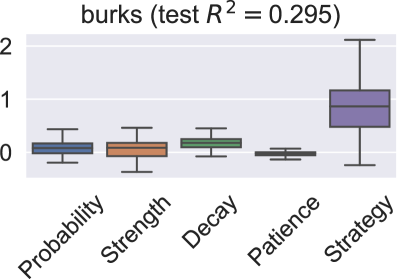
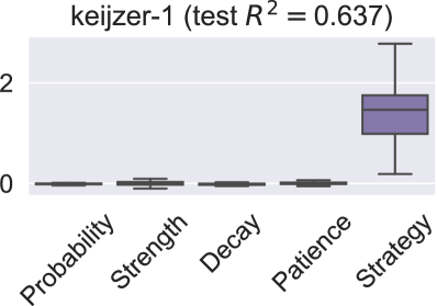
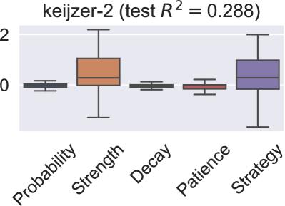
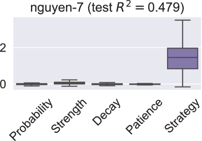
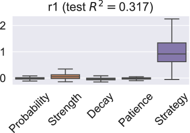
Figure 2. Hyper-parameter importance for the data sets upon which random forest learns a decent mapping (test $R^{2}>0.25$) between hyper-parameter setting and respective training performance of GP-GOMEA. Note that a negative values are due to random permutations used to estimate hyper-parameter importance leading to improved random forest test $R^{2}$ (less likely for good values of test $R^{2}>0.25$).

Before proceeding, we provide examples of why random forest did not learn a meaningful mapping between GP-GOMEA’s coefficient mutation hyper-parameter setting and its training performance for most data sets. Since the coefficient mutation strategy is the most important hyper-parameter from Fig. 2, we keep this hyper-parameter variable, while we fix the others, to a good setting (we explain how this is obtained in the next paragraph), namely probability of $1$, strength temperature-based with $\tau=0.1$, decay of $0.1$ with patience of $5$ generations. Now, Fig. 3 shows how performance changes according to the strategy when the other hyper-parameters are fixed as just mentioned, for three of the data sets for which the random forest’s test $R^{2}<0.25$. As it can be seen, GP-GOMEA obtains limited differences in performance when varying the strategy of coefficient mutation for different reasons. Conversely, Fig. 4 shows that the strategy has an impact on three of the data sets for which random forest obtained $R^{2}\geq 0.25$.

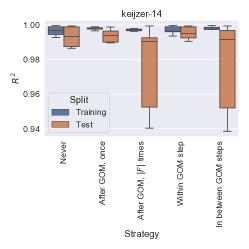
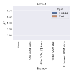
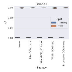
Figure 3. GP-GOMEA’s performance for three data sets for which it was not possible to learn how hyper-parameter settings influence (training) performance. The hyper-parameters are set to the best configuration found, expect for strategy, which is varied. In all cases, the (training) performance differences are too small across settings. Left: the runs found relatively good solutions. Middle: the runs always found perfect solutions. Right: the runs never found good solutions.

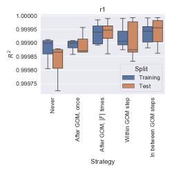
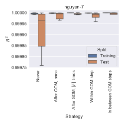
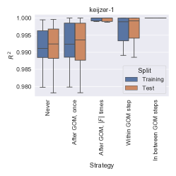
Figure 4. GP-GOMEA’s performance for three data sets for which it was possible to learn how hyper-parameter settings influence (training) performance. The hyper-parameters are set to the best configuration found, expect for strategy, which is varied.

Finally, we consider the five data sets of Fig. 2 and we look at the hyper-parameter settings that lead to top $15\%$ training performance. The result is shown separately for hyper-parameter and data set in Fig. 5, and jointly across both in Fig. 6. Two configurations appear to be most promising, which have in common the in between GOM steps strategy, probability of $1$, strength temperature-based with $\tau=0.1$, and patience of $5$ generations, while decay can be set to $0.1$ or $0.9$. We pick the decay of $0.1$ and proceed with the next experiment.

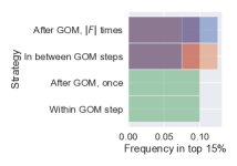
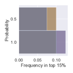
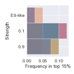
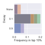
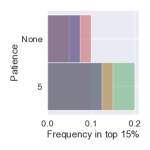
Figure 5. Frequency with which a coefficient mutation hyper-parameter setting appears in the top 15% of training performance, for the data sets burks, keijzer-1, keijzer-2, nguyen-7, and r1.

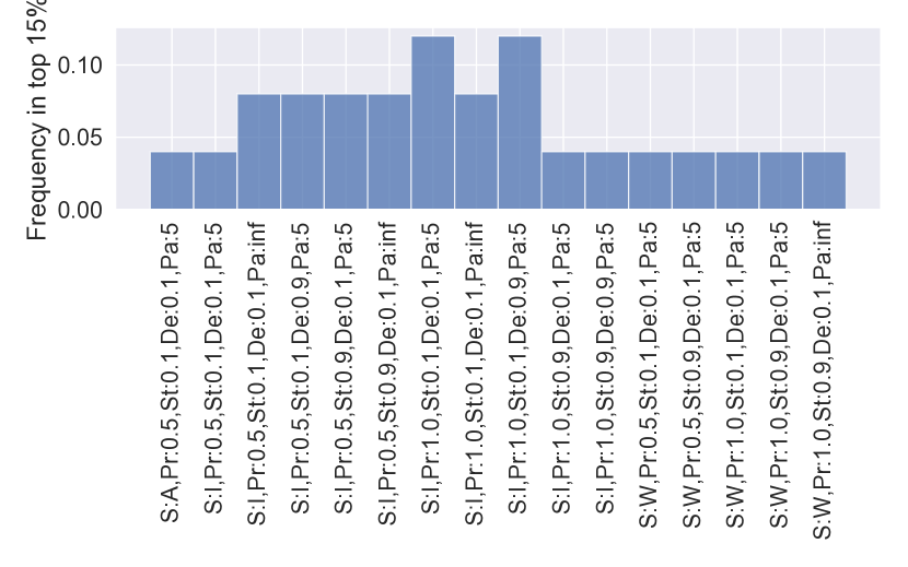
Figure 6. Frequency with which a hyper-parameter configuration appears among the top 15% of training performance obtained by GP-GOMEA. The abbreviations S:A, S:I, and S:W stand for strategy set to after GOM —FOS— times, in between GOM steps, and within GOM steps, respectively. The other abbreviations stand for, in order, probability, strength, decay, and patience.

6. Experiment 2: Application to SRBench

We use the promising hyper-parameter configuration from the previous experiment and proceed with benchmarking GP-GOMEA with coefficient mutation on the so-called ground-truth data sets of SRBench. These data sets were generated from a known, ground-truth equation, with varying level of noise added to the target variable (see (La Cava et al., 2021) for details). Here, we evaluate two options for the depth of the template tree (hereon simply referred to as depth, for brevity), i.e., $4$ and $6$, and two options for coefficient mutation, i.e., active (using the promising configuration) or inactive. Note that the current results for GP-GOMEA reported in (La Cava et al., 2021) and on the repository of SRBench use a depth of $6$ and no coefficient mutation.

We begin by considering the test $R^{2}$ obtained by the evolved models, as shown in Fig. 7 (see (La Cava et al., 2021) for full names and descriptions of the competing algorithms). All four configurations of GP-GOMEA perform very competitively, with rather small differences in terms of $R^{2}$ across different noise levels. Coefficient mutation seems not to make a large difference here. To get a more complete view, in Fig. 8 we report the solution rate, i.e., the frequency (out of ten repetitions) with which the algorithms re-discover the ground-truth equations from which the data set was generated. There, two configurations of GP-GOMEA achieve better results, namely the one using a depth of $6$ and inactive coefficient mutation, and the one using a depth of $4$ and active coefficient mutation. Regarding the other two configurations, using a depth of 6 and active coefficient mutation perform worse because it requires the largest number of evaluations (SRBench uses a budget of $1\,000\,000$ evaluations), while using a depth of 4 and inactive coefficient mutation makes it hard for GP-GOMEA to refine the models, which are necessarily small due to the constrained template size.

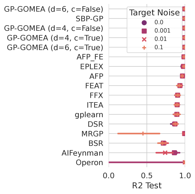
Figure 7. Test $R^{2}$ for the variants of GP-GOMEA and other algorithms currently benchmarked in SRBench. The large error bar of Operon is due to an outlier.

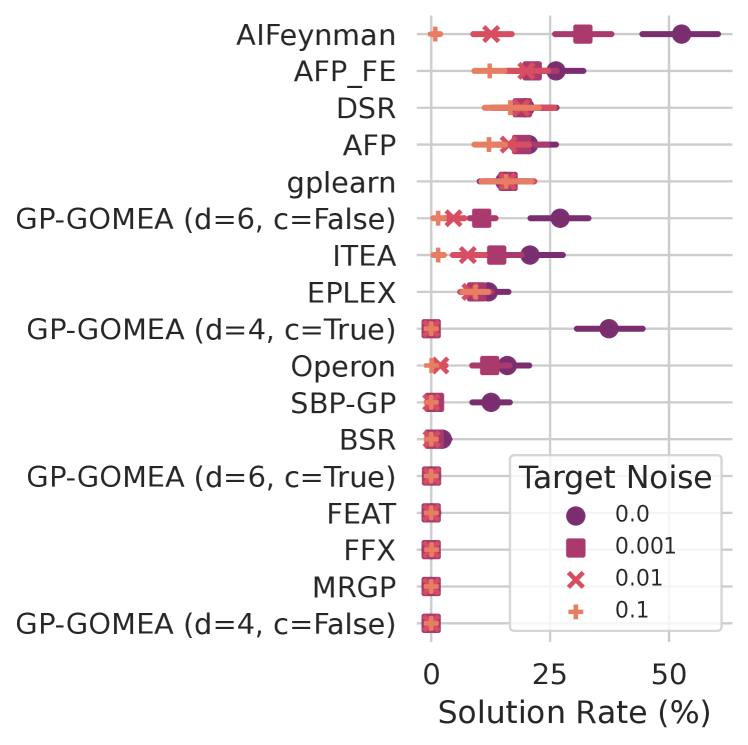
Figure 8. Rate with which an algorithm discovers the ground-truth equation from which the data set was generated, for the variants of GP-GOMEA and other algorithms currently benchmarked in SRBench.

Interestingly, despite having a smaller template for representing solutions, GP-GOMEA with depth of 4 and active coefficient mutation can be competitive with GP-GOMEA with depth of 6 and inactive coefficient mutation, at least when no noise is added to the target variable. Actually, without noise, coefficient mutation allows to substantially improve the discovery of the ground-truth equation, by approximately $+10\%$ (compared to GP-GOMEA with depth 6 and inactive coefficient mutation). However, when noise is added to the target, coefficient mutation makes GP-GOMEA dramatically less reliable in discovering the ground-truth equation.

7. Discussion

As variation in GP-GOMEA works differently than in GP, we investigated different strategies that determine at what stage and for how many attempts coefficient mutation should be applied in GP-GOMEA. In our first experiment (Sec. 5), we found that the choice of this strategy is typically the most important factor at play; at least for the data sets in which coefficient mutation plays a substantial role. The best strategy we found is to apply coefficient mutation in between every step of GOM. However, good results were also observed when applying coefficient mutation after all GOM steps had taken place, as long as the number of attempts matched those of GOM (i.e., the size of the FOS). In particular, applying coefficient mutation only a single time after an offspring is generated is not sufficient in GP-GOMEA.

Other hyper-parameter settings concerning coefficient mutation are generally less important. The temperature-based way of determining the strength of coefficient mutation, at least for the experimental setup we used (e.g., with the evaluation budget of SRBench), performed slightly better than the ES-like approach. However, the ES-like approach has the appeal that it requires less hyper-parameters to be set, and is likely to reach similar performance if more budget is given thanks to its self-adaptation. In particular, for this approach, it suffices that $\epsilon$ is a small number (we used $10^{-16}$), but a better choice of $\gamma$ may be important (we used $0.1$). We remark that the orders of magnitude for the sampling variance used in the ES-like approach and in the temperature-based approach at initialization can be dissimilar but not wildly so. With our choice of $\gamma$, we obtained that, at initialization, the sampling variance is approximately $1$ for all constant nodes (see Eqs. 2 and 3). For the temperature-based approach the sampling variance depends on $\tau$ and the current value of the coefficient $c$ (which is initialized according to the formula in Table 1). For a constant initialized at, e.g., $-5$ or $+10$, then using $\tau=0.1$ (found to perform best in Sec. 5) leads to a sampling variance of $0.25$ or $1$, respectively.

A downside of coefficient mutation (compared to, e.g., gradient descent) is that changes may often be detrimental. Therefore, one needs to evaluate whether the quality of a solution does improve after coefficient mutation, and roll back detrimental changes (at least in a stochastic manner). Under the assumption that node-wise recombination plays a key role in GP(-GOMEA), we did not investigate the effect of having more evaluations being spent for coefficient mutation instead of recombination (GOM). However, it may be important to study such scenarios, and of course to include other approaches for coefficient optimization. (Stochastic) gradient descent is a prime candidate for the future studies.

To understand the dynamics of coefficient mutation with respect to noisy measurements and discovery of ground-truth equations, we must consider Fig. 7 and Fig. 8 at the same time. This comparison reveals that, when noise is present, GP-GOMEA with (depth 4 and) active coefficient mutation discovers decently accurate models that, however, do not match the ground-truth equations. So, on the one hand, coefficient mutation allows for good models to be found under a relatively restrained representation (template tree with depth 4 compared to 6). On the other hand, coefficient mutation makes GP-GOMEA more susceptible to overfitting to noise. This begs the question as to whether the use of coefficient mutation (or coefficient optimization in general) should be accompanied with the use of some form of regularization, to reduce the chance of overfitting to (noise in) the training set.

8. Conclusion

Tuning coefficients can be important to tackle symbolic regression effectively. In this paper, we investigated how some simple, gradient-free forms of coefficient optimization can be integrated in GP-GOMEA, a state-of-the-art algorithms for symbolic regression. We have carried out two sets of experiments, on two different benchmark sets. In the first experiment, we have found that coefficient mutation does not always make a difference; however, when it does, then its most important factor is the strategy used to apply it. In GP-GOMEA, the amount of coefficient mutation attempts needs to be commensurate to the amount of recombination attempts. In the second experiment, we applied different variants of GP-GOMEA with and without coefficient mutation to the part of the SRBench benchmark that concerns discovering ground-truth equations from data. We have found that coefficient mutation enhances GP-GOMEA’s discovery success rate only if the data does not include noise. With noisy data, coefficient mutation leads to finding different equations than the ground-truth ones, which however are similarly accurate.

References

- (1)
- Babovic and Keijzer (2000) Vladan Babovic and Maarten Keijzer. 2000. Genetic programming as a model induction engine. Journal of Hydroinformatics 2, 1 (2000), 35–60.
- Beyer and Schwefel (2002) Hans-Georg Beyer and Hans-Paul Schwefel. 2002. Evolution strategies–A comprehensive introduction. Natural Computing 1, 1 (2002), 3–52.
- Biggio et al. (2021) Luca Biggio, Tommaso Bendinelli, Alexander Neitz, Aurelien Lucchi, and Giambattista Parascandolo. 2021. Neural Symbolic Regression that Scales. In International Conference on Machine Learning. PMLR, 936–945.
- Bottou (2010) Léon Bottou. 2010. Large-scale machine learning with stochastic gradient descent. In Proceedings of COMPSTAT. Springer, 177–186.
- Breiman (2001) Leo Breiman. 2001. Random forests. Machine Learning 45, 1 (2001), 5–32.
- Cranmer et al. (2020) Miles Cranmer, Alvaro Sanchez Gonzalez, Peter Battaglia, Rui Xu, Kyle Cranmer, David Spergel, and Shirley Ho. 2020. Discovering symbolic models from deep learning with inductive biases. Advances in Neural Information Processing Systems 33 (2020), 17429–17442.
- d’Ascoli et al. (2022) Stéphane d’Ascoli, Pierre-Alexandre Kamienny, Guillaume Lample, and François Charton. 2022. Deep Symbolic Regression for Recurrent Sequences. arXiv preprint arXiv:2201.04600 (2022).
- de França (2018) Fabrício Olivetti de França. 2018. A greedy search tree heuristic for symbolic regression. Information Sciences 442 (2018), 18–32.
- Dick et al. (2020) Grant Dick, Caitlin A Owen, and Peter A Whigham. 2020. Feature standardisation and coefficient optimisation for effective symbolic regression. In Proceedings of the Genetic and Evolutionary Computation Conference. 306–314.
- Evett and Fernandez (1998) Matthew Evett and Thomas Fernandez. 1998. Numeric mutation improves the discovery of numeric constants in genetic programming. Genetic Programming (1998), 66–71.
- Hein et al. (2018) Daniel Hein, Steffen Udluft, and Thomas A Runkler. 2018. Interpretable policies for reinforcement learning by genetic programming. Engineering Applications of Artificial Intelligence 76 (2018), 158–169.
- Howard and D’Angelo (1995) Les M Howard and Donna J D’Angelo. 1995. The GA-P: A genetic algorithm and genetic programming hybrid. IEEE Expert 10, 3 (1995), 11–15.
- Izzo et al. (2017) Dario Izzo, Francesco Biscani, and Alessio Mereta. 2017. Differentiable genetic programming. In European Conference on Genetic Programming. Springer, 35–51.
- Kadra et al. (2021) Arlind Kadra, Marius Lindauer, Frank Hutter, and Josif Grabocka. 2021. Well-tuned Simple Nets Excel on Tabular Datasets. Advances in Neural Information Processing Systems 34 (2021).
- Kammerer et al. (2020) Lukas Kammerer, Gabriel Kronberger, Bogdan Burlacu, Stephan M Winkler, Michael Kommenda, and Michael Affenzeller. 2020. Symbolic regression by exhaustive search: Reducing the search space using syntactical constraints and efficient semantic structure deduplication. In Genetic Programming Theory and Practice XVII. Springer, 79–99.
- Kantor et al. (2021) Daniel Kantor, Fernando J Von Zuben, and Fabricio Olivetti de Franca. 2021. Simulated annealing for symbolic regression. In Proceedings of the Genetic and Evolutionary Computation Conference. 592–599.
- Keijzer (2003) Maarten Keijzer. 2003. Improving symbolic regression with interval arithmetic and linear scaling. In European Conference on Genetic Programming. Springer, 70–82.
- Kommenda et al. (2020) Michael Kommenda, Bogdan Burlacu, Gabriel Kronberger, and Michael Affenzeller. 2020. Parameter identification for symbolic regression using nonlinear least squares. Genetic Programming and Evolvable Machines 21, 3 (2020), 471–501.
- Koza (1994) John R Koza. 1994. Genetic programming as a means for programming computers by natural selection. Statistics and Computing 4, 2 (1994), 87–112.
- La Cava et al. (2021) William La Cava, Patryk Orzechowski, Bogdan Burlacu, Fabrício Olivetti de França, Marco Virgolin, Ying Jin, Michael Kommenda, and Jason H Moore. 2021. Contemporary symbolic regression methods and their relative performance. arXiv preprint arXiv:2107.14351 (2021).
- La Cava et al. (2018) William La Cava, Tilak Raj Singh, James Taggart, Srinivas Suri, and Jason H Moore. 2018. Learning concise representations for regression by evolving networks of trees. In International Conference on Learning Representations.
- Langdon and Nordin (2000) William B Langdon and JP Nordin. 2000. Seeding genetic programming populations. In European Conference on Genetic Programming. Springer, 304–315.
- McConaghy (2011) Trent McConaghy. 2011. FFX: Fast, scalable, deterministic symbolic regression technology. In Genetic Programming Theory and Practice IX. Springer, 235–260.
- Medvet et al. (2018) Eric Medvet, Alberto Bartoli, Andrea De Lorenzo, and Fabiano Tarlao. 2018. GOMGE: Gene-pool optimal mixing on grammatical evolution. In International Conference on Parallel Problem Solving from Nature. Springer, 223–235.
- Miller and Smith (2006) Julian F Miller and Stephen L Smith. 2006. Redundancy and computational efficiency in cartesian genetic programming. IEEE Transactions on Evolutionary Computation 10, 2 (2006), 167–174.
- Moré (1978) Jorge J Moré. 1978. The Levenberg-Marquardt algorithm: Implementation and theory. In Numerical Analysis. Springer, 105–116.
- Nelder and Mead (1965) John A Nelder and Roger Mead. 1965. A simplex method for function minimization. The computer journal 7, 4 (1965), 308–313.
- Oliveira et al. (2018) Luiz Otavio VB Oliveira, Joao Francisco BS Martins, Luis F Miranda, and Gisele L Pappa. 2018. Analysing symbolic regression benchmarks under a meta-learning approach. In Proceedings of the Genetic and Evolutionary Computation Conference Companion. 1342–1349.
- Petersen et al. (2019) Brenden K Petersen, Mikel Landajuela Larma, T Nathan Mundhenk, Claudio P Santiago, Soo K Kim, and Joanne T Kim. 2019. Deep symbolic regression: Recovering mathematical expressions from data via risk-seeking policy gradients. arXiv preprint arXiv:1912.04871 (2019).
- Poli et al. (2008) Riccardo Poli, William B Langdon, Nicholas F McPhee, and John R Koza. 2008. A Field Guide to Genetic Programming. (2008).
- Rivero et al. (2022) Daniel Rivero, Enrique Fernandez-Blanco, and Alejandro Pazos. 2022. DoME: A deterministic technique for equation development and Symbolic Regression. Expert Systems with Applications (2022), 116712.
- Sadowski et al. (2016) Krzysztof L Sadowski, Peter AN Bosman, and Dirk Thierens. 2016. Learning and exploiting mixed variable dependencies with a model-based EA. In IEEE Congress on Evolutionary Computation. IEEE, 4382–4389.
- Sadowski et al. (2018) Krzysztof L Sadowski, Dirk Thierens, and Peter AN Bosman. 2018. GAMBIT: A parameterless model-based evolutionary algorithm for mixed-integer problems. Evolutionary Computation 26, 1 (2018), 117–143.
- Schmidt and Lipson (2009) Michael Schmidt and Hod Lipson. 2009. Distilling free-form natural laws from experimental data. science 324, 5923 (2009), 81–85.
- Thierens (2010) Dirk Thierens. 2010. The linkage tree genetic algorithm. In International Conference on Parallel Problem Solving from Nature. Springer, 264–273.
- Topchy and Punch (2001) Alexander Topchy and W. F. Punch. 2001. Faster Genetic Programming Based on Local Gradient Search of Numeric Leaf Values. In Proceedings of the Genetic and Evolutionary Computation Conference. Morgan Kaufmann Publishers Inc., San Francisco, CA, USA, 155–162.
- Trujillo et al. (2014) Leonardo Trujillo, Oliver Schütze, and Pierrick Legrand. 2014. Evaluating the effects of local search in genetic programming. In EVOLVE-A Bridge between Probability, Set Oriented Numerics, and Evolutionary Computation V. Springer, 213–228.
- Udrescu and Tegmark (2020) Silviu-Marian Udrescu and Max Tegmark. 2020. AI Feynman: A physics-inspired method for symbolic regression. Science Advances 6, 16 (2020), eaay2631.
- Van Laarhoven and Aarts (1987) Peter JM Van Laarhoven and Emile HL Aarts. 1987. Simulated annealing. In Simulated annealing: Theory and applications. Springer, 7–15.
- Virgolin et al. (2017) Marco Virgolin, Tanja Alderliesten, Cees Witteveen, and Peter AN Bosman. 2017. Scalable genetic programming by gene-pool optimal mixing and input-space entropy-based building-block learning. In Proceedings of the Genetic and Evolutionary Computation Conference. 1041–1048.
- Virgolin et al. (2021) Marco Virgolin, Tanja Alderliesten, Cees Witteveen, and Peter AN Bosman. 2021. Improving model-based genetic programming for symbolic regression of small expressions. Evolutionary Computation 29, 2 (2021), 211–237.
- Virgolin et al. (2022) Marco Virgolin, Eric Medvet, Tanja Alderliesten, and Peter AN Bosman. 2022. Less is More: A Call to Focus on Simpler Models in Genetic Programming for Interpretable Machine Learning. arXiv preprint arXiv:2204.02046 (2022).
- Zhang and Smart (2005) Mengjie Zhang and Will Smart. 2005. Learning weights in genetic programs using gradient descent for object recognition. In Workshops on Applications of Evolutionary Computation. Springer, 417–427.