Fractional Brownian Gyrator

Abstract

When a physical system evolves in a thermal bath at a constant temperature, it arrives eventually to an equilibrium state whose properties are independent of the kinetic parameters and of the precise evolution scenario. This is generically not the case for a system driven out of equilibrium which, on the contrary, reaches a steady-state with properties that depend on the full details of the dynamics such as the driving noise and the energy dissipation. How the steady state depends on such parameters is in general a non-trivial question. Here, we approach this broad problem using a minimal model of a two-dimensional nano-machine, the Brownian gyrator, that consists of a trapped particle driven by fractional Gaussian noises – a family of noises with long-ranged correlations in time and characterized by an anomalous diffusion exponent $\alpha$. When the noise is different in the different spatial directions, our fractional Brownian gyrator persistently rotates. Even if the noise is non-trivial, with long-ranged time correlations, thanks to its Gaussian nature we are able to characterize analytically the resulting nonequilibrium steady state by computing the probability density function, the probability current, its curl and the angular velocity and complement our study by numerical results.

1 Introduction

The Brownian gyrator model, that consists of a pair of coupled, standardly defined Ornstein-Uhlenbeck processes each evolving at its own temperature, is one of the simplest models exhibiting a non-trivial out-of-equilibrium dynamics and, for this reason, has received much interest in the last two decades. It was originally introduced as a solvable model of dynamics with two temperatures [1], and it was realized only years later that a systematic torque is generated on the object [2], so that it can be seen as a minimal nano-machine that, on average, undergoes steady gyration around the origin. Following this remarkable observation, various facets of the model have been studied in different contexts. In addition to the theoretical calculation of the evolution of some relevant properties (see e.g. Refs. [3, 4, 5, 6, 7]), several more general questions have also been addressed including the role of cross-correlations between different degrees of freedom coupled to different thermostats on the production of entropy [8], the directionality of interactions between cellular processes [9], statistical properties of the energy exchanged between two heat baths in electric circuits [10, 11] and their spectral properties [12], dynamics in suspensions of two types of particles exposed to different heat baths [13] and in laser-cooled atomic gases [14], as well as the synchronization of out-of-equilibrium Kuramoto oscillators [15]. Furthermore, exerting external forces on a Brownian gyrator has lead to derive a special fluctuation theorem and to identify associated effective temperatures [16, 12, 17]. The latter setting with external forces was found to be mathematically equivalent to the bead-spring model studied via Brownian dynamics simulations in Ref. [18] and analytically in Refs. [19, 20]. Finally, different versions of a Brownian gyrator were studied experimentally, especially from the point of view of fluctuation relations [10, 11, 21].

All the above-mentioned analyses concentrated exclusively on situations in which the noise acting on both components of the gyrator is thermal and delta-correlated in time. However, nano-machines can be encountered or engineered in a variety of environments including active suspensions [22, 23] or complex biological mediums [24] where the noise is athermal and correlated in time. It is thus important to understand the effects of correlated noise on the Brownian gyrator. A first step was made recently in Ref. [25] which considered persistent noise that is exponentially correlated in time and the associated memory kernel for the damping so that, individually, the noise on each component remains thermal. Even for such short-ranged correlations, essential departures from the standard white noise model emerge which raise the question of the effect of other types of noise, athermal and/or with long-ranged time correlations. From a broader perspective, because of its simplicity, the Brownian gyrator model is an ideal playground to understand the effects of different types of noise correlations on the properties of a nonequilibrium steady state.

In the present paper, we tackle the question formulated above by generalizing the Brownian gyrator model to a fractional Brownian gyrator (FBG) in which the noise acting on each component is the so-called fractional Gaussian noise (FGN) [26]. The latter, in fact, represent a family of colored noises parametrized by an anomalous diffusion exponent $\alpha$ such that an overdamped particle in free space subject to a FGN performs the standard fractional Brownian motion [26, 27]. When $\alpha<1$ the increments are anti-correlated and the dynamics is sub-diffusive whereas for $\alpha>1$ the increments are positively correlated which entails a super-diffusive motion. The standard Brownian gyrator model is recovered in the borderline case when $\alpha=1$. Our analysis here covers all three situations within a unified framework, so that we can inquire for each type of correlations if they are beneficial or, on the contrary, detrimental to rotation. In any case, rotation can appear only if the symmetry between the two spatial components is broken. Here, to assess independently the different features of the noise, we discuss especially two situations: In the first case, both noises have the same $\alpha$ but different amplitudes while in the second case the amplitudes are equal while the values of $\alpha$ differ. We calculate exactly the probability density function $P(x,y;t)$ and present its explicit form in the limit $t\to\infty$. We further compute the probability current, its curl, and eventually calculate the ensemble-averaged angular velocity. For each quantity, we compare our results to numerical simulations.

The paper is outlined as follows: We first introduce the dynamics and detail the two variants of the model that breaks the symmetry using different parameters in Sec. 2. In Sec. 3 we compute analytically the first moments of the position before giving the full probability density function and considering numerical applications. We further compute some important quantities characterizing the nonequilibrium steady state in Sec. 4: the probability current, its curl and the mean angular velocity. Finally, we summarize our findings in Sec. acknowledgments. Details of intermediate calculations are relegated to Appendices.

2 The Model

2.1 Definition

Let us first present the standard Brownian gyrator (BG) as introduced in Ref. [1]. We denote by $x(t)$ and $y(t)$ the Cartesian coordinates of an overdamped particle evolving in a potential $U(x,y)$ according to the Langevin equation

$$\gamma\dot{x}(t) =-\partial_{x}U(x,y)+\xi_{x}(t)$$ (1)

$$\gamma\dot{y}(t) =-\partial_{y}U(x,y)+\xi_{y}(t)\,,$$

where $\gamma$ is the damping coefficient, $U(x,y)=(1/2)(k_{x}x^{2}+k_{y}y^{2})-uxy$ is a generic harmonic potential and $\xi_{x}(t)$ and $\xi_{y}(t)$ are additive Gaussian white noises with zero mean. Adopting appropriate space and time units, we can choose without loss of generality $k_{x}=k_{y}=1$ and $\gamma=1$ so that the dynamics rewrite

$$\dot{x}(t) =-x(t)+uy(t)+\xi_{x}(t)$$ (2)

$$\dot{y}(t) =-y(t)+ux(t)+\xi_{y}(t)\,.$$

with noise variance

$$\langle\xi_{i}(t_{1})\xi_{j}(t_{2})\rangle=2T_{j}\delta_{i,j}\delta(t_{1}-t_{2})\,,\qquad i,j=x,y\,.$$ (3)

We are interested in the case when the particle is trapped, which requires $|u|<1$. When $T_{x}\neq T_{y}$, the system is out of equilibrium and exhibits a persistent rotation in steady state [2].

In this paper, we generalize the BG model by considering the situation in which $\xi_{x}(t)$ and $\xi_{y}(t)$ are two fractional Gaussian noises (FGNs) with different parameters so that their correlation function reads

$$\langle\xi_{i}(t_{1})\xi_{j}(t_{2})\rangle=T_{j}\delta_{ij}N_{\alpha_{j}}(t_{1},t_{2})\,.$$ (4)

The kernel $N_{\alpha_{j}}(t_{1},t_{2})$ is defined such that in free space, $\dot{x}_{\rm free}=\xi_{x}(t)$ yields the so-called fractional Brownian for $x_{\rm free}$ (see, e.g., [31]):

$$\langle x_{\rm free}(t_{1})x_{\rm free}(t_{2})\rangle =T_{x}\int_{0}^{t_{1}}\textrm{d}\tau_{1}\int_{0}^{t_{2}}\textrm{d}\tau_{2}\,N_{\alpha x}(\tau_{1},\tau_{2})$$

$$=T_{x}(t_{1}^{\alpha}+t_{2}^{\alpha}-|t_{1}-t_{2}|^{\alpha})\,.$$ (5)

In particular, the mean squared displacement exhibits an anomalous diffusion

$$\langle x_{\rm free}^{2}(t)\rangle=2T_{x}t^{\alpha}\,,$$ (6)

where $\alpha\in(0,2)$ is the anomalous diffusion exponent. $\alpha=1$ corresponds to the standard Brownian motion while $\alpha<1$ and $\alpha>1$ generate sub-diffusion and super-diffusion respectively. The explicit expression of the kernel $N_{\alpha_{j}}$ that satisfies Eq. (5) for arbitrary $\alpha\in(0,2)$ is not needed for the calculations presented in this paper. The interested reader can find detailed discussions on this topic in Refs.[31, 28, 29, 32].

Let us note that, although in the following we will call abusively $T_{x}$ and $T_{y}$ “temperatures”, one should keep in mind that they are not physical temperatures but rather only the noise amplitudes. Indeed, even if the components are independent ($u=0$), each component is out of equilibrium since the noise and damping do not satisfy the fluctuation-dissipation theorem, except when $\alpha=1$.

Numerical simulations are performed by solving Eq. (2) using an Euler–Maruyama algorithm. The FGN is generated by using the Davies and Harte method [33] and is provided by the Stochastic python module.

2.2 Two variants

Although all our analytical results can be derived for the general FBG introduced above, it will help to discuss specifically two variants of the model in which we vary different parameters. In the first one (Model 1) the anomalous diffusion exponent is unique, $\alpha_{x}=\alpha_{y}\equiv\alpha$, but the temperatures $T_{x}$ and $T_{y}$ are different, so that the noise correlations read

$${\rm Model\,1:}\qquad\langle\xi_{x}(t_{1})\xi_{x}(t_{1})\rangle=T_{x}N_{\alpha}(t_{1},t_{2})\,,\qquad\langle\xi_{y}(t_{1})\xi_{y}(t_{1})\rangle=T_{y}N_{\alpha}(t_{1},t_{2})\,.$$ (7)

In Model 2, the temperature $T_{x}=T_{y}\equiv T$ is the same for both components but the anomalous diffusion exponents are different, so that

$${\rm Model\,2:}\qquad\langle\xi_{x}(t_{1})\xi_{x}(t_{1})\rangle=TN_{\alpha_{x}}(t_{1},t_{2})\,,\qquad\langle\xi_{y}(t_{1})\xi_{y}(t_{1})\rangle=TN_{\alpha_{y}}(t_{1},t_{2})\,.$$ (8)

3 Spatial distribution

We first solve the equations of motion for a given realization of the noise which will allow us to obtain any moment of the position distribution. Thanks to their linear structure, the equations of motion Eq. (2) are readily integrated to give

$$x(t) =\int_{0}^{t}\textrm{d}\tau\,Q_{c}(t-\tau)\xi_{x}(\tau)+\int_{0}^{t}\textrm{d}\tau\,Q_{s}(t-\tau)\xi_{y}(\tau)$$ (9)

$$y(t) =\int_{0}^{t}\textrm{d}\tau\,Q_{s}(t-\tau)\xi_{x}(\tau)+\int_{0}^{t}\textrm{d}\tau\,Q_{c}(t-\tau)\xi_{y}(\tau)\,,$$

with the kernels

$$Q_{c}(t)=\textrm{e}^{-t}\cosh(ut)\,,\qquad Q_{s}(t)=\textrm{e}^{-t}\sinh(ut)\,.$$ (10)

For simplicity, and since we are interested only in the steady-state properties, we chose the initial condition $x(0)=y(0)=0$. Since the noises have zero mean it follows that $\langle x(t)\rangle=\langle y(t)\rangle=0$ at all time.

In the following, we first compute the second moment of the position in Sec. 3.1 and the full probability density function in Sec. 3.2 and analyze quantitatively the effect of the FGN on the spatial distribution in Sec. 3.3.

3.1 Mean squared displacement and cross correlations

The second moments of the position distribution can be computed at all time from Eq. (9) and the expression of the noise correlation Eq. (5). They take the form

$$\langle x^{2}(t)\rangle =A_{x}(t)T_{x}+B_{y}(t)T_{y}$$ (11)

$$\langle y^{2}(t)\rangle =B_{x}(t)T_{x}+A_{y}(t)T_{y}$$ (12)

$$\langle x(t)y(t)\rangle =C_{x}(t)T_{x}+C_{y}(t)T_{y}\,,$$ (13)

where $A_{j}(t)$, $B_{j}(t)$, and $C_{j}(t)$ are given by the following integrals

$$A_{j}(t) =\int_{0}^{t}\textrm{d}\tau_{1}\int_{0}^{t}\textrm{d}\tau_{2}\,Q_{c}(t-\tau_{1})Q_{c}(t-\tau_{2})N_{\alpha_{j}}(\tau_{1},\tau_{2})$$ (14)

$$B_{j}(t) =\int_{0}^{t}\textrm{d}\tau_{1}\int_{0}^{t}\textrm{d}\tau_{2}\,Q_{s}(t-\tau_{1})Q_{s}(t-\tau_{2})N_{\alpha_{j}}(\tau_{1},\tau_{2})$$ (15)

$$C_{j}(t) =\int_{0}^{t}\textrm{d}\tau_{1}\int_{0}^{t}\textrm{d}\tau_{2}\,Q_{c}(t-\tau_{1})Q_{s}(t-\tau_{2})N_{\alpha_{j}}(\tau_{1},\tau_{2})\,,$$ (16)

where $j=x,y$ and to compute $C_{j}(t)$, we have used the symmetry $N_{\alpha_{j}}(\tau_{1},\tau_{2})=N_{\alpha_{j}}(\tau_{2},\tau_{1})$. Since we are interested in the nonequilibrium steady state (NESS), we evaluate the quantities in Eqs. (14)-(16) in the limit $t\rightarrow\infty$. Details of the derivation can be found in A. Eventually, we find

$$A_{j} =\frac{\Gamma(1+\alpha_{j})}{4}\biggl{[}\frac{2-u}{(1-u)^{\alpha_{j}}}+\frac{2+u}{(1+u)^{\alpha_{j}}}\biggr{]}$$ (17)

$$B_{j} =\frac{\Gamma(1+\alpha_{j})}{4}\biggl{[}\frac{u}{(1-u)^{\alpha_{j}}}-\frac{u}{(1+u)^{\alpha_{j}}}\biggr{]}$$ (18)

$$C_{j} =\frac{\Gamma(1+\alpha_{j})}{4}\biggl{[}\frac{1}{(1-u)^{\alpha_{j}}}-\frac{1}{(1+u)^{\alpha_{j}}}\biggr{]}\,.$$ (19)

where $A_{j},B_{j},C_{j}$ denote the limiting values of $A_{j}(t),B_{j}(t),C_{j}(t)$ in the limit $t\to\infty$.

One can notice that the asymptotic values of $A_{j}$, $B_{j}$ and $C_{j}$ are finite (exist) only for $|u|<1$. This is the only case of interest to us. When $|u|\geq 1$, the physics is very different since the particle is not trapped, a fact which is reflected in the diverging mean-squared displacements along both directions as $t\to\infty$.

3.2 Probability density function and characteristic function

Since the noise is Gaussian and the equations of motion are linear, the probability density function $P(x,y;t)$ is fully determined by the second moments. This is most concisely expressed using the characteristic function

$$\Phi(t,\lambda_{x},\lambda_{y};T_{x},T_{y};\alpha_{x},\alpha_{y}) =\langle\textrm{e}^{{\rm i}\lambda_{x}x(t)+{\rm i}\lambda_{y}y(t)}\rangle$$

$$=\exp\Bigl{[}-\frac{1}{2}\left(\langle x^{2}(t)\rangle\lambda_{x}^{2}+\langle y^{2}(t)\rangle\lambda_{y}^{2}+2\langle x(t)y(t)\rangle\lambda_{x}\lambda_{y}\right)\Bigr{]}\,,$$ (20)

where $\langle x^{2}(t)\rangle$, $\langle y^{2}(t)\rangle$, and $\langle x(t)y(t)\rangle$ are given by Eqs. (11)-(13). The calculation of the characteristic function Eq. (3.2) is performed in B.

The probability density function is then obtained as the inverse Fourier transform of Eq. (3.2), which gives

$$P(x,y;t)=\frac{1}{2\pi\sqrt{\langle x^{2}(t)\rangle\langle y^{2}(t)\rangle-\langle x(t)y(t)\rangle^{2}}}\exp\biggl{[}-\frac{\langle y^{2}(t)\rangle x^{2}+\langle x^{2}(t)\rangle y^{2}-2\langle x(t)y(t)\rangle xy}{2(\langle x^{2}(t)\rangle\langle y^{2}(t)\rangle-\langle x(t)y(t)\rangle^{2})}\biggr{]}\,.$$ (21)

The normalization $\int_{\mathbb{R}^{2}}\textrm{d}x\textrm{d}y\,P(x,y;t)=1$ is ensured since the condition $\langle x^{2}(t)\rangle\langle y^{2}(t)\rangle>\langle x(t)y(t)\rangle^{2}$ is satisfied as long as the moments remain finite.

Integrating Eq. (21) over one variable, the marginal distributions $P(x;t)$ and $P(y;t)$ take the expected form

$$P(x;t)=\frac{1}{\sqrt{2\pi\langle x^{2}(t)\rangle}}\textrm{e}^{-\frac{x^{2}}{2\langle x^{2}(t)\rangle}};\quad P(y;t)=\frac{1}{\sqrt{2\pi\langle y^{2}(t)\rangle}}\textrm{e}^{-\frac{y^{2}}{2\langle y^{2}(t)\rangle}}\,.$$ (22)

3.3 Quantitative analysis of the effect of the FGN

We discuss here the effect of the FGN on the position moments in the special cases of Model 1 and 2.

In Model 1, which has $\alpha_{x}=\alpha_{y}$ and $T_{x}\neq T_{y}$, the second moments Eq. (11)-(13) in the steady state simplify to

$$\langle x^{2}\rangle =\frac{\Gamma(1+\alpha)}{4}\left[2\left(\frac{1}{(1-u)^{\alpha}}+\frac{1}{(1+u)^{\alpha}}\right)T_{x}+u\left(\frac{1}{(1-u)^{\alpha}}-\frac{1}{(1+u)^{\alpha}}\right)(T_{x}-T_{y})\right]$$

$$\langle xy\rangle =\frac{\Gamma(1+\alpha)}{4}\left(\frac{1}{(1-u)^{\alpha}}-\frac{1}{(1+u)^{\alpha}}\right)(T_{x}-T_{y})$$ (23)

and $\langle y^{2}\rangle$ is obtained by interchanging $T_{x}$ and $T_{y}$ in the expression for $\langle x^{2}\rangle$. Putting $\alpha=1$, one recovers the results of Ref[3, 14]. Fig. 1 shows the prediction of Eq. (23) for varying $\alpha$. Comparing with numerical simulations confirms that the predictions are exact. We observe that, varying $\alpha$, the shape of the curves is not affected. However, quantitatively, $\alpha$ has a strong effect. In particular, the dependence on $u$ becomes much steeper when $\alpha$ increases, with the amplitude of all quantities increasing by more than an order of magnitude for all $|u|>0.5$ when increasing $\alpha$ from $0.2$ to $1.6$.

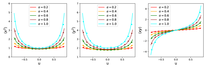
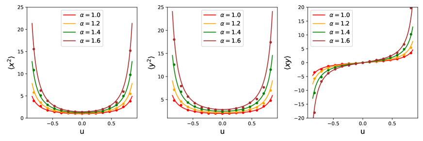
Figure 1: Model $1$: $\langle x^{2}\rangle$, $\langle y^{2}\rangle$ and $\langle xy\rangle$ versus $u$ for varying $\alpha$. $T_{x}=1$ and $T_{y}=2$. We separated the sub-diffusive case (top) and the super-diffusive case (bottom) for readability. Full curves correspond to the exact results and dots to the simulation data.

When $u=0$, we find, as expected, that the two components decouple, i.e. $\langle xy\rangle=0$. The variance becomes $\langle x^{2}\rangle=\Gamma(1+\alpha)T_{x}$ so that we can interpret $\Gamma(1+\alpha)T_{x}\equiv T_{\rm eff,x}$ as an effective temperature and the marginal distribution $P(x)\propto e^{-x^{2}/(2T_{\rm eff,x})}$ as an effective Boltzmann distribution although the system remains out of equilibrium as discussed in Sec. 2.

For Model 2, which has $T_{x}=T_{y}$ and $\alpha_{x}\neq\alpha_{y}$, Figure 2 shows the moments $\langle x^{2}\rangle$, $\langle y^{2}\rangle$ and $\langle xy\rangle$ as functions of the anisotropy parameter $u$ when increasing the difference in exponent while keeping $\alpha_{x}=2-\alpha_{y}$. We see that increasing the difference in exponent from $0$ to $1.2$, the amplitude of all quantities increases, more significantly as $|u|$ gets larger, although the effect remains moderate.

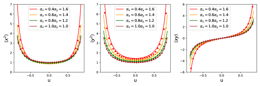
Figure 2: Model $2$: $\langle x^{2}\rangle$, $\langle y^{2}\rangle$ and $\langle xy\rangle$ versus $u$ with $T_{x}=T_{y}=1$ and varying difference in the exponent $\alpha_{x}=2-\alpha_{y}$. Full curves correspond to the exact results and dots to the simulation data.

4 Currents and rotation

A NESS is characterized by the existence of a probability current. We first compute this steady-state current in Sec. 4.1. We then use it to characterize the rotational motion of our gyrator through the angular velocity in Sec. 4.2 and the curl of the current in Sec. 4.3.

4.1 Steady-state current

Computing the current for our FBG involves subtleties due to the fact that for the noises with long-ranged temporal correlations, we cannot write a closed-form differential equation for the probability density function which would generalize the Fokker-Planck equation that can be written when $\alpha=1$ and give us an expression of the current. We circumvent here this fundamental difficulty by starting directly from the definition of the current $\textbf{J}(x,y,t)=(J_{x}(x,y,t),J_{y}(x,y,t))$ as an ensemble-average over noise realizations

$$J_{x}(x,y;t) = \langle\dot{x}(t)\delta(x-x(t))\delta(y-y(t))\rangle$$ (24)

$$J_{y}(x,y;t) = \langle\dot{y}(t)\delta(x-x(t))\delta(y-y(t))\rangle\,.$$ (25)

It is easy to check that this is a good definition of the current, in the sense that it satisfies the continuity equation $\partial_{t}P(x,y,t)+\nabla\cdot\textbf{J}(x,y,t)=0$.

Using the integral representation of the Dirac delta function, $J_{x}$ can be expressed as

$$J_{x}(x,y;t)=\int_{\mathbb{R}^{2}}\frac{\textrm{d}\lambda_{x}\textrm{d}\lambda_{y}}{(2\pi)^{2}}\textrm{e}^{-{\rm i}x\lambda_{x}-{\rm i}y\lambda_{y}}\langle\dot{x}(t)\textrm{e}^{{\rm i}\lambda_{x}x(t)+{\rm i}\lambda_{y}y(t)}\rangle\,.$$ (26)

which becomes, using the equation of motion Eq. (2),

$$J_{x}(x,y;t)=\int_{\mathbb{R}^{2}}\frac{\textrm{d}\lambda_{x}\textrm{d}\lambda_{y}}{(2\pi)^{2}}\textrm{e}^{-{\rm i}x\lambda_{x}-{\rm i}y\lambda_{y}}\langle\bigl{[}-x(t)+uy(t)+\xi_{x}(t)\Bigr{]}\textrm{e}^{{\rm i}\lambda_{x}x(t)+{\rm i}\lambda_{y}y(t)}\rangle\,.$$ (27)

The average containing the first two terms on the r.h.s. can be computed by using the characteristic function

$$\langle x(t)\textrm{e}^{{\rm i}\lambda_{x}x(t)+{\rm i}\lambda_{y}y(t)}\rangle=-{\rm i}\partial_{\lambda_{x}}\Phi(t,\lambda_{x},\lambda_{y})\,;\quad\langle y(t)\textrm{e}^{{\rm i}\lambda_{x}x(t)+{\rm i}\lambda_{y}y(t)}\rangle=-{\rm i}\partial_{\lambda_{y}}\Phi(t,\lambda_{x},\lambda_{y})\,.$$ (28)

with $\Phi(t,\lambda_{x},\lambda_{y})$ (we have omitted the dependence on the other parameters for brevity) given in B.1. The last term requires different characteristic functions

$$\Xi_{x}=\langle\xi_{x}(t)\textrm{e}^{{\rm i}\lambda_{x}x(t)+{\rm i}\lambda_{y}y(t)}\rangle;\qquad\Xi_{y}=\langle\xi_{y}(t)\textrm{e}^{{\rm i}\lambda_{x}x(t)+{\rm i}\lambda_{y}y(t)}\rangle\,,$$ (29)

which are given in B.2.

Putting everything together (see details in C) we arrive at the following expression for the current in steady state

$$J_{x}(x,y) =-P(x,y)\partial_{x}U(x,y)-\Gamma(1+\alpha_{x})T_{x}\partial_{x}P(x,y)$$ (30)

$$J_{y}(x,y) =-P(x,y)\partial_{y}U(x,y)-\Gamma(1+\alpha_{y})T_{y}\partial_{y}P(x,y)\,.$$ (31)

We recognize the effective temperatures $T_{\rm eff,x/y}=\Gamma(1+\alpha_{x/y})T_{x/y}$ introduced in Sec. 3.3 which control the probability distribution at $u=0$ when the two components are decoupled. In addition, we see from Eq. (30) that for any $u$ the relation between current and probability is the same as the one that would be obtained for a standard Brownian gyrator driven by Gaussian white noises at the effective temperatures $T_{\rm eff,x/y}$.

The current field is shown in Fig. 3 for the special case of Model 1 with $T_{x}=1$, $T_{y}=2$ and $u=0.3$ and two values of $\alpha$. Interestingly, one observes that when $\alpha$ becomes larger, the symmetry axis of the current rotates.

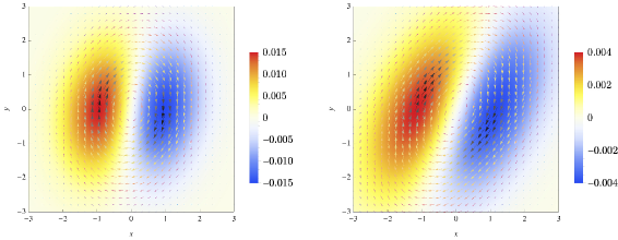
Figure 3: Model 1: Current field with arrows indicating the direction and the color map indicating the amplitude. Left panel: $\alpha=0.5$. Right panel: $\alpha=1.5$. In both panels $T_{x}=1$, $T_{y}=2$, $u=0.3$.

4.2 Angular velocity

One can use the expression Eq. (30) for the current to compute the steady-state angular velocity

$$\langle{\bm{\omega}}\rangle=\int d^{2}{\bf r}\,\,\frac{1}{r^{2}}{\bf r}\land{\bf J}$$ (32)

Since the current vector belongs to the $xy$ plane, we write $\langle{\bm{\omega}}\rangle=\langle\omega\rangle{\bf\hat{z}}$ and, after straightforward algebra, we obtain the explicit, although lengthy, expression:

$$\langle\omega\rangle =\Bigg{(}T_{x}\Gamma(1+\alpha_{x})F(u,\alpha_{x})-T_{y}\Gamma(1+\alpha_{y})F(u,\alpha_{y})\Bigg{)}$$

$$\quad\Bigg{/}\Bigg{(}H(\alpha_{x},u)(T_{x}\Gamma(1+\alpha_{x}))^{2}+H(\alpha_{y},u)(T_{y}\Gamma(1+\alpha_{y}))^{2}$$

$$\qquad+2M(\alpha_{x},\alpha_{y},u)T_{x}T_{y}\Gamma(1+\alpha_{x})\Gamma(1+\alpha_{y})\Bigg{)}^{1/2}\,,$$ (33)

where

$$F(u,\alpha) =(1+u)^{2-\alpha}-(1-u)^{2-\alpha}$$ (34)

$$H(u,\alpha) =-(1+u)^{2-2\alpha}-(1-u)^{2-2\alpha}+2(1+u^{2})(1-u^{2})^{-\alpha}$$ (35)

$$M(\alpha_{x},\alpha_{y},u) =(1+u)^{2-\alpha_{x}-\alpha_{y}}+(1-u)^{2-\alpha-\alpha_{y}}$$

$$+(3-u^{2})\left((1+u)^{-\alpha_{x}}(1-u)^{-\alpha_{y}}+(1-u)^{-\alpha_{x}}(1+u)^{-\alpha_{y}}\right)$$ (36)

As for the standard BG, one needs a double symmetry breaking (geometric and in the noise) to observe a rotation. Indeed, one sees from Eq. (4.2) that the angular velocity vanishes if either $u=0$ or if $\alpha_{x}=\alpha_{y}$ and $T_{x}=T_{y}$.

On the contrary, as soon as both symmetry breakings are present, one observes a rotation in general. This is most clearly seen by performing a series expansion $\langle\omega\rangle$ in powers of $u$ to simplify Eq. (4.2) to

$$\langle\omega\rangle=\frac{T_{x}\Gamma(1+\alpha_{x})(2-\alpha_{x})-T_{y}\Gamma(1+\alpha_{y})(2-\alpha_{y})}{2\sqrt{T_{x}T_{y}\Gamma(1+\alpha_{x})\Gamma(1+\alpha_{y})}}u+O(u^{3})$$ (37)

At this order, the second symmetry breaking occurs when

$$T_{y}\Gamma(1+\alpha_{y})(2-\alpha_{y})\neq T_{x}\Gamma(1+\alpha_{x})(2-\alpha_{x}).$$ (38)

This result encompasses the cases of both Models 1 and 2, showing that rotation is generated by having either different temperatures or different exponents. Conversely, rotation can be diminished, even with different noises, by choosing the parameters so that Eq. (38) becomes an equality.

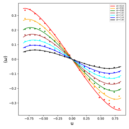
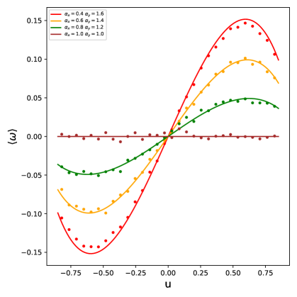
Figure 4: Mean angular velocity as function of the anisotropy parameter $u$. Left: Model 1 with $T_{x}=1$ and $T_{y}=2$. Right: Model 2 with $T_{x}=T_{y}=1$.

Let us now discuss the predictions of Eq. (4.2) and compare with numerical measurements. In practice, we do not use Eq. (32) to compute the angular velocity in simulations but rather compute the time derivative of the polar angle. The mean of $\omega$ is displayed in Fig. 4 for Model 1 and Model 2. For Model 1, we observe that $\langle\omega\rangle$ becomes larger as the asymmetry $|u|$ increases and as $\alpha$ decreases. For Model 2, $\langle\omega\rangle$ shows two extrema with $|u|$ and increases in amplitude when the difference between the exponents increases.

4.3 Curl of the current

The rotational motion of the particle in the NESS can also be characterized by the curl of the current ${\bf\nabla}\land{\bf J}$ which can be computed from Eq. (30). In particular, let us give here its expression at the origin in the case of Model 1

$${\bf\nabla}\land{\bf J}(0,0)=\frac{T_{x}^{2}-T_{y}^{2}}{4\pi(T_{x}T_{y})^{3/2}}\frac{(1-u^{2})^{\alpha/2}}{\Gamma(1+\alpha)}\frac{G_{+}(2u,u,\alpha)}{[1+G_{-}(1+u^{2},u,\alpha)\Delta^{2}]^{3/2}}$$ (39)

where

$$G_{\pm}(x,u,\alpha)=\frac{x}{2}+\frac{1-u^{2}}{4}\biggl{[}-\left(\frac{1+u}{1-u}\right)^{\alpha-1}\pm\left(\frac{1-u}{1+u}\right)^{\alpha-1}\biggr{]};\quad\Delta=\frac{T_{y}-T_{x}}{2\sqrt{T_{x}T_{y}}}\,.$$ (40)

Again one can see the double symmetry breaking that is necessary to obtain a rotational motion since ${\bf\nabla}\land{\bf J}(0,0)$ in Eq. (39) vanishes when either $T_{x}=T_{y}$ or $u=0$. The known result for the Brownian gyrator [3],

$${\bf\nabla}\land{\bf J}_{\rm BG}(0,0)=\frac{T_{x}^{2}-T_{y}^{2}}{4\pi(T_{x}T_{y})^{3/2}}\frac{u\sqrt{1-u^{2}}}{(1+u^{2}\Delta^{2})^{3/2}}\,,$$ (41)

is easily retrieved by observing that $G_{+}(2u,u,1)=u$ and $G_{-}(1+u^{2},u,1)=u^{2}$.

Fig. 5 shows the curl at the origin for various temperatures and two exponents. One observes that the extrema depend little on the temperature but strongly on $\alpha$, increasing by an order of magnitude when going from $\alpha=1.75$ to $\alpha=0.25$. The latter trend is also observed on the current field and its curl at arbitrary positions, displayed in Fig. 6.

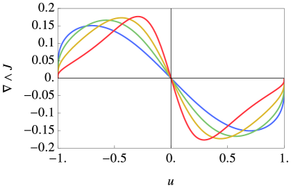
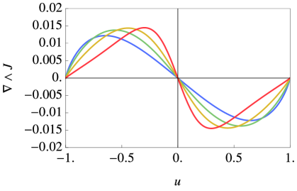
Figure 5: Model 1: ${\bf\nabla}\land{\bf J}(0,0)$ as a function of $u$ for $T_{y}$ taking values $5$ (blue), $10$ (green), $20$ (dark yellow), and $50$ (red). Left panel: $\alpha=0.25$. Right panel: $\alpha=1.75$. $T_{x}=1$.

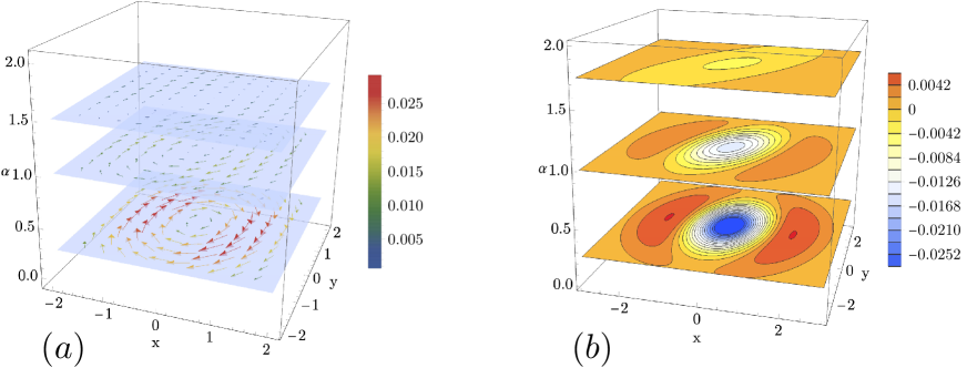
Figure 6: Model 1: Panel (a) the current field $\mathbb{J}(x,y)$ in the steady state. The vertical slices are taken at $\alpha=0.25$, $\alpha=1$ and $\alpha=1.75$. Panel (b): the $z$-component of $\nabla\wedge\textbf{J}(x,y)$ at the same values of $\alpha$. For both panels: $T_{x}=1$, $T_{y}=2$, $u=0.5$

In the case of Model 2, unsurprisingly, the curl at the origin increases when the difference between the exponents increase, as illustrated in Fig. 7.

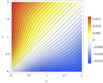
Figure 7: Model 2: Density plot of ${\bf\nabla}\land{\bf J}(0,0)$ as a function of $\alpha_{x}$, $\alpha_{y}$ with $T=1$ and $u=0.1$. The curl vanishes for $\alpha_{x}=\alpha_{y}$ (dashed line).

5 Conclusion

We have considered the two-dimensional motion of a particle in a harmonic potential. The particle undergoes Brownian motion in the overdamped limit under the action of different fractional Gaussian noises along the two spatial directions. As such it is out of equilibrium and display a non-vanishing current in steady state. Most strikingly, the particle rotates around the origin. This model can be seen as a minimal model of a nonequilibrium steady state driven by long-range correlated noise that can be tuned to be sub-diffusive or super-diffusive. We have computed analytically the full position probability distribution and the current in steady state, from which we deduced the angular velocity and the curl of the current characterizing the rotational motion of the particle. Numerical simulations confirmed these derivations in two special cases where the rotation is driven either by different amplitudes of the noise or by different exponents. The effect of the fractional noise, compared to the white noise case $\alpha=1$ is rather paradoxical: When decreasing $\alpha$ the position distribution becomes more and more insensitive to the asymmetry $u$ but at the same time the current and angular velocity increase. For large values of $\alpha$, the particle probability becomes much more spread and sensitive to the asymmetry but rotates slower around the origin.

Of course, the properties of the nonequilibrium steady-state that we have determined here depend on the details of the dynamics. For example, we expect that using a generalized Langevin equation as in Ref. [25] but including power-law correlations instead of exponential ones will lead to a different steady state compared to our result even though the free dynamics of each component is exactly the same in both models (see e.g. [28, 29, 30]). Long-ranged correlated non-Gaussian noise could also yield different results. However, there is hope that some universality is at play and that, qualitatively, our conclusions capture the effect of long-ranged time correlations beyond a specific model. It would be interesting to question this universality by studying other models in the future or even by comparing to experimental measurements.

Appendix A Auxiliary functions

The calculation of $A_{j}(t)$, $B_{j}(t)$, and $C_{j}(t)$ involves integrals of the following form

$$g_{\alpha}(t)=\int_{0}^{t}\textrm{d}t_{1}\int_{0}^{t}\textrm{d}t_{2}\,\omega_{1}(t-t_{1})\omega_{2}(t-t_{2})N_{\alpha}(t_{1},t_{2})\,,$$ (42)

the choice of the kernel $\omega_{j}$ depending on the specific function one is considering. We use the fact that

$$N_{\alpha}(t_{1},t_{2})=\partial_{t_{1}}\partial_{t_{2}}\mathcal{G}_{\alpha}(t_{1},t_{2})\,,$$ (43)

where

$$\mathcal{G}_{\alpha}(t_{1},t_{2})=\left(t_{1}^{\alpha}+t_{2}^{\alpha}-|t_{1}-t_{2}|^{\alpha}\right)$$ (44)

is the autocorrelation function in free space. Integrating by parts twice we find an expression for $g_{\alpha}(t)$

$$g_{\alpha}(t) =\omega_{1}(0)\omega_{2}(0)\mathcal{G}_{\alpha}(t,t)+\omega_{1}(0)\int_{0}^{t}\textrm{d}t_{2}\,\omega_{2}^{\prime}(t-t_{2})\mathcal{G}_{\alpha}(t,t_{2})+\omega_{2}(0)\int_{0}^{t}\textrm{d}t_{1}\,\omega_{1}^{\prime}(t-t_{1})\mathcal{G}_{\alpha}(t_{1},t)$$

$$+\int_{0}^{t}\textrm{d}t_{1}\int_{0}^{t}\textrm{d}t_{2}\,\omega_{1}^{\prime}(t-t_{1})\omega_{2}^{\prime}(t-t_{2})\mathcal{G}_{\alpha}(t_{1},t_{2})\,,$$ (45)

where $\omega^{\prime}(u)\equiv\textrm{d}\omega(u)/\textrm{d}u$.

A.1 The function $A_{j}(t)$

For the function $A_{j}(t)$ the kernel is given by $\omega_{1}(t)=\omega_{2}(t)=Q_{c}(t)$. The first term in the right hand side of Eq. (A) yields the contribution $2t^{\alpha}$ because $Q_{c}(0)=1$. The terms involving a single integration are identical and their contribution is denoted $A_{j}^{(\rm I)}(t)$. Then, the contribution stemming from the term involving a double integral is denoted $A_{j}^{(\rm II)}(t)$. Hence,

$$A_{j}(t)=2t^{\alpha}+A_{j}^{(\rm I)}(t)+A_{j}^{(\rm II)}(t)\,,$$ (46)

with

$$A_{j}^{(\rm I)}(t)=2\int_{0}^{t}\textrm{d}t_{1}\,Q_{c}^{\prime}(t-t_{1})\mathcal{G}_{\alpha}(t,t_{1})\,.$$ (47)

Recalling that $Q_{c}^{\prime}(t)=[u\sinh(ut)-\cosh(ut)]e^{-t}$, the change of variables $t-t_{1}=zt$ gives

$$A_{j}^{(\rm I)}(t)=2t^{1+\alpha}\int_{0}^{1}\textrm{d}z\,\Bigl{[}u\sinh(utz)-\cosh(utz)\Bigr{]}\exp(-tz)\bigl{[}1+(1-z)^{\alpha}-z^{\alpha}\bigr{]}\,.$$ (48)

It is convenient to express the integral in terms of the function

$$F(q,\alpha)=\int_{0}^{1}\textrm{d}z\,\exp(-qz)\bigl{[}1+(1-z)^{\alpha}-z^{\alpha}\bigr{]}\,.$$ (49)

Therefore

$$A_{j}^{(\rm I)}(t)=-t^{1+\alpha}\biggl{[}(1-u)F((1-u)t,\alpha)+(1+u)F((1+u)t,\alpha)\biggr{]}\,.$$ (50)

Since we are interested in $\lim_{t\rightarrow\infty}A_{j}(t)$, it is sufficient to consider the infinite-$q$ limit of the function $F(q,\alpha)$ for positive $q$. In such a limit we can use the asymptotic expansion

$$F(q,\alpha)=\frac{2}{q}-\frac{\Gamma(1+\alpha)}{q^{1+\alpha}}-\frac{\alpha}{q^{2}}+O(q^{-3})\,,\qquad q\rightarrow\infty\,.$$ (51)

Taking $0<u<1$, it follows that

$$A_{j}^{(\rm I)}(t)=-4t^{\alpha}+\frac{2\alpha}{1-u^{2}}t^{\alpha-1}+\Gamma(1+\alpha)\biggl{[}\frac{1}{(1-u)^{\alpha}}+\frac{1}{(1+u)^{\alpha}}\biggr{]}+O(t^{\alpha-2})\,.$$ (52)

Let us consider now the contribution from the double integral

$$A_{j}^{(\rm II)}(t)=\int_{0}^{t}\textrm{d}t_{1}\int_{0}^{t}\textrm{d}t_{2}\,Q_{c}^{\prime}(t-t_{1})Q_{c}^{\prime}(t-t_{2})\mathcal{G}_{\alpha}(t_{1},t_{2})\,.$$ (53)

We further split $A_{j}^{(\rm II)}(t)$ into a contribution due to the terms $t_{1}^{\alpha}+t_{2}^{\alpha}$ in $\mathcal{G}_{\alpha}(t_{1},t_{1})$ and the remainder due to $|t_{1}-t_{2}|^{\alpha}$. This splitting is denoted as follows

$$A_{j}^{(\rm II)}(t)=A_{j}^{(\rm II,1)}(t)+A_{j}^{(\rm II,2)}(t)\,,$$ (54)

with

$$A_{j}^{(\rm II,1)}(t)=\int_{0}^{t}\textrm{d}t_{1}\int_{0}^{t}\textrm{d}t_{2}\,Q_{c}^{\prime}(t-t_{1})Q_{c}^{\prime}(t-t_{2})\left(t_{1}^{\alpha}+t_{2}^{\alpha}\right)\,,$$ (55)

and

$$A_{j}^{(\rm II,2)}(t)=-\int_{0}^{t}\textrm{d}t_{1}\int_{0}^{t}\textrm{d}t_{2}\,Q_{c}^{\prime}(t-t_{1})Q_{c}^{\prime}(t-t_{2})|t_{1}-t_{2}|^{\alpha}\,,$$ (56)

The integrals in Eq. (55) are factorized, therefore

$$A_{j}^{(\rm II,1)}(t) =2\int_{0}^{t}\textrm{d}t_{1}\,t_{1}^{\alpha}Q_{c}^{\prime}(t-t_{1})\int_{0}^{t}\textrm{d}t_{2}\,Q_{c}^{\prime}(t-t_{2})\,.$$ (57)

The integration yields

$$A_{j}^{(\rm II,1)}(t)=\left(-1+\textrm{e}^{-t}\cosh(ut)\right)\biggl{[}\phi_{\alpha}((1-u)t)+\phi_{\alpha}((1+u)t)\biggr{]}t^{\alpha}\,,$$ (58)

where

$$\phi_{\alpha}(z)=\textrm{e}^{-{\rm i}\pi\alpha}z^{-\alpha}\textrm{e}^{-z}(\Gamma(\alpha+1)-\Gamma(\alpha+1,-z))\,.$$ (59)

When $z\rightarrow+\infty$ we have

$$\phi_{\alpha}(z)=-1+\frac{\alpha}{z}+O(z^{-2})\,,\qquad z\rightarrow+\infty\,.$$ (60)

Focusing on those terms which in the large-$t$ expansion are not exponentially suppressed, we find

$$A_{j}^{(\rm II,1)}(t)=2t^{\alpha}-\frac{2\alpha}{1-u^{2}}t^{\alpha-1}+O(t^{\alpha-2})\,.$$ (61)

We can now consider the integral Eq. (56), which can be written in the form

$$A_{j}^{(\rm II,2)}(t)=-\int_{0}^{t}\textrm{d}t_{1}\,Q_{c}^{\prime}(t_{1})\int_{0}^{t}\textrm{d}t_{2}\,Q_{c}^{\prime}(t_{2})|t_{1}-t_{2}|^{\alpha}\,,$$ (62)

which follows by applying the change of variables $t_{1}\rightarrow t-t_{1}$ and $t_{2}\rightarrow t-t_{2}$ in Eq. (56). Since the correlation function $\mathcal{G}_{\alpha}(t_{1},t_{2})$ is invariant under the interchange of $t_{1}$ and $t_{2}$, we have

$$A_{j}^{(\rm II,2)}(t)=-2\int_{0}^{t}\textrm{d}t_{1}\,Q_{c}^{\prime}(t_{1})\int_{0}^{t_{1}}\textrm{d}t_{2}\,Q_{c}^{\prime}(t_{2})(t_{1}-t_{2})^{\alpha}\,.$$ (63)

Again, since we are interested in the large-$t$ behavior, we can simply perform a Laplace transform with respect to $t$ and apply the final value theorem. The Laplace transform is written as follows

$$\mathcal{L}\left(A_{j}^{(\rm II,2)}(t);t,s\right)=-\frac{2}{s}\int_{0}^{\infty}\textrm{d}t_{1}\,\textrm{e}^{-st_{1}}Q_{c}^{\prime}(t_{1})\int_{0}^{t_{1}}\textrm{d}t_{2}\,Q_{c}^{\prime}(t_{2})(t_{1}-t_{2})^{\alpha}\,,$$ (64)

where $s$ is the Laplace parameter. The integrations in Eq. (64) can be computed analytically and the corresponding result admits the following Taylor expansion for small $s$

$$\mathcal{L}\left(A_{j}^{(\rm II,2)}(t);t,s\right)=-\frac{2}{s}\sum_{n=0}^{\infty}a_{n}(u,\alpha)s^{n}\,,$$ (65)

where $a_{n}(u,\alpha)$ are functions that can be determined analytically. The final value theorem states that

$$\lim_{t\rightarrow\infty}A_{j}^{(\rm II,2)}(t)=\lim_{s\rightarrow 0}s\mathcal{L}\left(A_{j}^{(\rm II,2)}(t);t,s\right)\,,$$ (66)

and therefore

$$\lim_{t\rightarrow\infty}A_{j}^{(\rm II,2)}(t)=-2a_{0}(u,\alpha)\,\quad\text{with}\quad a_{0}(u,\alpha)=\frac{\Gamma(1+\alpha)}{8}\biggl{[}\frac{2+u}{(1-u)^{\alpha}}+\frac{2-u}{(1+u)^{\alpha}}\biggr{]}\,.$$ (67)

Let us mention that it is also possible to invert the Laplace transform in Eq. (63) and obtain the formal expansion for large $t$, including also the subleading corrections for large times. Collecting the results obtained so far, we find

$$\lim_{t\rightarrow\infty}A_{j}(t)=\frac{}{4}\Gamma(1+\alpha)\biggl{[}\frac{2-u}{(1-u)^{\alpha}}+\frac{2+u}{(1+u)^{\alpha}}\biggr{]}\,.$$ (68)

A.2 The function $B_{j}(t)$

The calculation of this function, which has kernels $\omega_{1}(t)=\omega_{2}(t)=Q_{s}(t)$, turns out to be easier than the calculation of $A_{j}(t)$ because $Q_{s}(t)$ vanishes at $t=0$. As a result,

$$B_{j}(t)=\int_{0}^{t}\textrm{d}t_{1}\int_{0}^{t}\textrm{d}t_{2}\,Q_{s}^{\prime}(t-t_{1})Q_{s}^{\prime}(t-t_{2})\mathcal{G}_{\alpha}(t_{1},t_{2})\,.$$ (69)

We proceed by following the very same guidelines which we followed for the calculation of $A_{j}(t)$. Using the same notation as before, we split Eq. (69) by writing

$$B_{j}(t)=B_{j}^{(\rm II,1)}(t)+B_{j}^{(\rm II,2)}(t)\,,$$ (70)

where

$$B_{j}^{(\rm II,1)}(t) =\int_{0}^{t}\textrm{d}t_{1}\int_{0}^{t}\textrm{d}t_{2}\,Q_{s}^{\prime}(t-t_{1})Q_{s}^{\prime}(t-t_{2})\left(t_{1}^{\alpha}+t_{2}^{\alpha}\right)\,,$$ (71)

$$B_{j}^{(\rm II,2)}(t) =-\int_{0}^{t}\textrm{d}t_{1}\int_{0}^{t}\textrm{d}t_{2}\,Q_{s}^{\prime}(t-t_{1})Q_{s}^{\prime}(t-t_{2})|t_{1}-t_{2}|^{\alpha}\,.$$ (72)

The first integral gives

$$B_{j}^{(\rm II,1)}(t) =2\int_{0}^{t}\textrm{d}t_{1}\,t_{1}^{\alpha}Q_{s}^{\prime}(t-t_{1})\int_{0}^{t}\textrm{d}t_{2}\,Q_{s}^{\prime}(t-t_{2})$$

$$=\sinh(ut)\textrm{e}^{-2t}\biggl{[}(1-u)^{-\alpha}\textrm{e}^{-i\pi\alpha+tu}(\Gamma(1+\alpha)-\Gamma(1+\alpha,-t(1-u)))$$

$$-(1+u)^{-\alpha}\textrm{e}^{-i\pi\alpha-tu}(\Gamma(1+\alpha)-\Gamma(1+\alpha,-t(1+u)))\biggr{]}$$

$$=\sinh(ut)\textrm{e}^{-t}t^{\alpha}\biggl{[}\phi_{\alpha}((1-u)t)-\phi_{\alpha}((1+u)t)\biggr{]}\,.$$ (73)

When $t\rightarrow\infty$ the function $\phi_{\alpha}$ reduces to a constant while the overall $t$-dependence $\sim\exp(-(1-u)t)$ produces

$$\lim_{t\rightarrow\infty}B_{j}^{(\rm II,1)}(t)=0\,.$$ (74)

The second integral in Eq. (71) is first written in the form

$$B_{j}^{(\rm II,2)}(t) =-\int_{0}^{t}\textrm{d}t_{1}\,Q_{s}^{\prime}(t-t_{1})\int_{0}^{t}\textrm{d}t_{2}\,Q_{s}^{\prime}(t-t_{2})|t_{1}-t_{2}|^{\alpha}$$

$$=-\int_{0}^{t}\textrm{d}t_{1}\,Q_{s}^{\prime}(t_{1})\int_{0}^{t}\textrm{d}t_{2}\,Q_{s}^{\prime}(t_{2})|t_{1}-t_{2}|^{\alpha}$$

$$=-2\int_{0}^{t}\textrm{d}t_{1}\,Q_{s}^{\prime}(t_{1})\int_{0}^{t_{1}}\textrm{d}t_{2}\,Q_{s}^{\prime}(t_{2})(t_{1}-t_{2})^{\alpha}\,.$$ (75)

We apply the Laplace transform of both sides

$$\mathcal{L}\left(B_{j}^{(\rm II,2)}(t);t,s\right)=-\frac{2}{s}\int_{0}^{\infty}\textrm{d}t_{1}\,\textrm{e}^{-st_{1}}Q_{s}^{\prime}(t-t_{1})\int_{0}^{t_{1}}\textrm{d}t_{2}\,Q_{s}^{\prime}(t-t_{2})|t_{1}-t_{2}|^{\alpha}\,,$$ (76)

and we get

$$\mathcal{L}\left(B_{j}^{(\rm II,2)}(t);t,s\right)=-\frac{2}{s}\sum_{n=0}^{\infty}b_{n}(u,\alpha)s^{n}\,;\quad b_{0}(u,\alpha)=\frac{u\Gamma(1+\alpha)}{8}\bigl{[}(1+u)^{-\alpha}-(1-u)^{-\alpha}\bigr{]}\,.$$ (77)

The final value theorem then allows us to write

$$\lim_{t\rightarrow\infty}B_{j}(t)=-2b_{0}(u,\alpha)=\frac{u\Gamma(1+\alpha)}{4}\bigl{[}(1-u)^{-\alpha}-(1+u)^{-\alpha}\bigr{]}\,.$$ (78)

A.3 The function $C_{j}(t)$

Now using kernels $\omega_{1}(t)=Q_{c}(t)$ and $\omega_{2}(t)=Q_{s}(t)$, we write as before

$$C_{j}(t) =C_{j}^{(\rm I)}(t)+C_{j}^{(\rm II)}(t)\,,$$

where

$$C_{j}^{(\rm I)}(t) =\int_{0}^{t}\textrm{d}t_{2}\,Q_{s}^{\prime}(t-t_{2})\mathcal{G}_{\alpha}(t,t_{2})$$ (79)

$$C_{j}^{(\rm II)}(t) =\int_{0}^{t}\textrm{d}t_{1}\int_{0}^{t}\textrm{d}t_{2}\,Q_{c}^{\prime}(t-t_{1})Q_{s}^{\prime}(t-t_{2})\mathcal{G}_{\alpha}(t_{1},t_{2})\,.$$ (80)

The first integral gives

$$C_{j}^{(\rm I)}(t)=\frac{1}{2}\Gamma(1+\alpha)\bigl{[}(1-u)^{-\alpha}-(1+u)^{-\alpha}\bigr{]}+\frac{1}{2}t^{\alpha}\Bigl{[}\phi_{\alpha}((1-u)t)-\phi_{\alpha}((1+u)t)\Bigr{]}\,,$$ (81)

and asymptotically it reduces to

$$C_{j}^{(\rm I)}(t)=\frac{1}{2}\Gamma(1+\alpha)\bigl{[}(1-u)^{-\alpha}-(1+u)^{-\alpha}\bigr{]}+\frac{\alpha u}{1-u^{2}}t^{\alpha-1}+O(t^{\alpha-2})\,.$$ (82)

We split the second integral as already done in the previous sections writing

$$C_{j}^{(\rm II)}(t)=C_{j}^{(\rm II,1)}(t)+C_{j}^{(\rm II,2)}(t)\,,$$ (83)

with

$$C_{j}^{(\rm II,1)}(t) =\int_{0}^{t}\textrm{d}t_{1}\,t_{1}^{\alpha}Q_{c}^{\prime}(t-t_{1})\int_{0}^{t}\textrm{d}t_{2}\,Q_{s}^{\prime}(t-t_{2})$$

$$+\int_{0}^{t}\textrm{d}t_{1}\,Q_{c}^{\prime}(t-t_{1})\int_{0}^{t}\textrm{d}t_{2}\,t_{2}^{\alpha}Q_{s}^{\prime}(t-t_{2})$$ (84)

and

$$C_{j}^{(\rm II,2)}(t) =-\int_{0}^{t}\textrm{d}t_{1}\int_{0}^{t}\textrm{d}t_{2}\,Q_{c}^{\prime}(t-t_{1})Q_{s}^{\prime}(t-t_{2})|t_{1}-t_{2}|^{\alpha}\,.$$

Up to exponentially small terms,

$$C_{j}^{(\rm II,1)}(t) \simeq\frac{1}{2}\bigl{[}-\phi_{\alpha}((1-u)t)+\phi_{\alpha}((1+u)t)\bigr{]}t^{\alpha}$$

$$\simeq-\frac{\alpha u}{1-u^{2}}t^{\alpha-1}+O(t^{\alpha-2})\,.$$ (85)

We can now consider $C_{j}^{(\rm II,2)}(t)$, which is given by

$$C_{j}^{(\rm II,2)}(t) =-\int_{0}^{t}\textrm{d}t_{1}\,\int_{0}^{t}\textrm{d}t_{2}\,Q_{c}^{\prime}(t_{1})Q_{s}^{\prime}(t_{2})|t_{1}-t_{2}|^{\alpha}\,.$$

In contrast with the functions $A_{j}^{(\rm II,2)}(t)$ and $C_{j}^{(\rm II,2)}(t)$, the integrand is not symmetric under the exchange of $t_{1}$ and $t_{2}$. This time, we approach the calculation by performing directly the Laplace transform and then integrating with respect to $t_{1}$ and $t_{2}$. The application of the final value theorem then gives

$$\lim_{t\rightarrow\infty}C_{j}^{(\rm II,2)}(t)=-\frac{}{4}\Gamma(1+\alpha)\Bigl{[}(1-u)^{-\alpha}-(1+u)^{-\alpha}\Bigr{]}\,.$$ (86)

Assembling all the pieces together, we finally obtain

$$\lim_{t\rightarrow\infty}C_{j}(t)=\frac{}{4}\Gamma(1+\alpha)\Bigl{[}(1-u)^{-\alpha}-(1+u)^{-\alpha}\Bigr{]}\,.$$ (87)

Appendix B Characteristic functions

Here we calculate the characteristic functions $\Phi$ and $Q_{j}$ which are defined in Eqs. (3.2) and (28), respectively.

B.1 The function $\Phi$

By inserting Eq. (9) into Eq. (3.2), and recalling that $\langle\xi_{x}(t_{1})\xi_{y}(t_{2})\rangle=0$, it follows that Eq. (3.2) can be factorized as follows

$$\Phi(t,\lambda_{x},\lambda_{y};T_{x},T_{y};\alpha_{x},\alpha_{y})=\Psi(t,\lambda_{x},\lambda_{y};T_{x};\alpha_{x})\Psi(t,\lambda_{y},\lambda_{x};T_{y};\alpha_{y})\,,$$ (88)

where

$$\Psi(t,\lambda_{x},\lambda_{y};T_{j};\alpha_{j})=\biggl{\langle}\exp\biggl{[}{\rm i}\int_{0}^{t}\textrm{d}\tau\,\left(\lambda_{x}Q_{c}(t-\tau)+\lambda_{y}Q_{s}(t-\tau)\right)\xi_{x}(\tau)\biggr{]}\biggr{\rangle}\,,\qquad j=x,y\,.$$ (89)

The second factor in the r.h.s. of Eq. (88) is obtained upon interchanging $\lambda_{x}$ with $\lambda_{y}$ and by using the appropriate values for the temperature and anomalous exponent. Since the noise is Gaussian, the characteristic function in Eq. (89) is completely determined by the second moment of the random process appearing in the argument of the exponential. It is formally given by

$$G(t,\lambda_{x},\lambda_{y};T_{j};\alpha_{j})=\biggl{\langle}\biggl{[}{\rm i}\int_{0}^{t}\textrm{d}\tau\,\left(\lambda_{x}Q_{c}(t-\tau)+\lambda_{y}Q_{s}(t-\tau)\right)\xi_{x}(\tau)\biggr{]}^{2}\biggr{\rangle}\,,$$ (90)

and therefore the characteristic function Eq. (89) is

$$\Psi(t,\lambda_{x},\lambda_{y};T_{j};\alpha_{j})=\exp\bigl{[}2^{-1}G(t,\lambda_{x},\lambda_{y};T_{j};\alpha_{j})\bigr{]}\,.$$ (91)

Eventually, we can write the quadratic form in $\lambda_{x}$, $\lambda_{y}$

$$G(t,\lambda_{x},\lambda_{y};T_{j};\alpha_{j}) =-T_{j}\Bigl{[}A_{x}(t)\lambda_{x}^{2}+B_{x}(t)\lambda_{y}^{2}+2C_{x}(t)\lambda_{x}\lambda_{y}\Bigr{]}\,,$$ (92)

By inserting Eq. (92) into Eq. (91), we have

$$\Psi(t,\lambda_{x},\lambda_{y};T_{j};\alpha_{j})=\exp\biggl{[}-\frac{T_{j}}{2}\left(A_{j}(t)\lambda_{x}^{2}+B_{j}(t)\lambda_{y}^{2}+2C_{j}(t)\lambda_{x}\lambda_{y}\right)\biggr{]}\,.$$ (93)

from which Eq. (3.2) is recovered using Eq. (88).

B.2 The function $\Xi_{j}$

In order to compute the characteristic function $\Xi_{j}$ it is instructive to consider a preliminary exercise which can be applied to the calculation of $\Xi_{j}$. Suppose that we want to compute the following characteristic function

$$\Omega(\mathcal{X},t)=\langle\xi_{x}(t)\textrm{e}^{{\rm i}(\mathcal{X}\star\xi_{x})_{t}}\rangle\,,$$ (94)

where $\xi_{x}(t)$ is the FGN, $\star$ denotes the convolution defined by

$$(\mathcal{X}\star\xi_{x})_{t}\equiv\int_{0}^{t}\textrm{d}\tau\,\mathcal{X}(t-\tau)\xi_{x}(\tau)\,,$$ (95)

and $\mathcal{X}$ is some kernel. The calculation of Eq. (94) is performed by expanding in power series the exponential and using the fact that only even powers of $\xi_{x}$ contributes in the averaging. Therefore

$$\Omega(\mathcal{X},t)=\sum_{n=0}^{\infty}\frac{{\rm i}^{2n+1}}{(2n+1)!}\langle\xi_{x}(t)\langle(\mathcal{X}\star\xi_{x})_{t})^{2n+1}\rangle\,.$$ (96)

The quantity in angular brackets can be computed by applying Wick’s theorem, which yields

$$\langle\xi_{x}(t)\langle(\mathcal{X}\star\xi_{x})_{t})^{2n+1}\rangle=(2n+1)!!\langle\xi_{x}(t)(\mathcal{X}\star\xi_{x})_{t})\rangle\Bigl{[}\langle(\mathcal{X}\star\xi_{x})_{t})^{2}\rangle\Bigr{]}^{n}\,,$$ (97)

by inserting Eq. (97) into Eq. (96),

$$\Omega(\mathcal{X},t)={\rm i}\langle\xi_{x}(t)(\mathcal{X}\star\xi_{x})_{t})\rangle\sum_{n=0}^{\infty}\frac{(2n+1)!!}{(2n+1)!}\Bigl{[}-\langle(\mathcal{X}\star\xi_{x})_{t})^{2}\rangle\Bigr{]}^{n}$$ (98)

Thanks to the identity

$$\frac{(2n+1)!!}{(2n+1)!}=\frac{1}{2^{n}n!}\,,$$ (99)

it follows that Eq. (98) is the Taylor expansion of the exponential. The summation of the series gives

$$\Omega(\mathcal{X},t)={\rm i}\langle\xi_{x}(t)(\mathcal{X}\star\xi_{x})_{t})\rangle\exp\biggl{[}-\frac{1}{2}\langle(\mathcal{X}\star\xi_{x})_{t})^{2}\rangle\biggr{]}\,.$$ (100)

We can now to carry out the calculation of the characteristic function $\Xi_{j}$. Let us start with $\Xi_{x}$,

$$\Xi_{x}=\langle\xi_{x}(t)\textrm{e}^{{\rm i}\lambda_{x}x(t)+{\rm i}\lambda_{y}y(t)}\rangle\,.$$ (101)

The quantity in the exponential can be factorized in two terms: the first contains $\xi_{x}$ and a second $\xi_{y}$

$$\Xi_{x} =\biggl{\langle}\xi_{x}(t)\exp\biggl{[}{\rm i}\int_{0}^{t}\textrm{d}\tau\,\left(\lambda_{x}Q_{c}(t-\tau)+\lambda_{y}Q_{s}(t-\tau)\right)\xi_{x}(\tau)\biggr{]}\biggr{\rangle}$$

$$\times\biggl{\langle}\exp\biggl{[}{\rm i}\int_{0}^{t}\textrm{d}\tau\,\left(\lambda_{y}Q_{c}(t-\tau)+\lambda_{x}Q_{s}(t-\tau)\right)\xi_{y}(\tau)\biggr{]}\biggr{\rangle}\,.$$ (102)

The second factor is precisely $\Psi(t,\lambda_{y},\lambda_{x};T_{y};\alpha_{y})$. The first factor has the form of Eq .(94) with the kernel $\mathcal{X}$ given by

$$\mathcal{X}(t-\tau)=\lambda_{x}Q_{c}(t-\tau)+\lambda_{y}Q_{s}(t-\tau)\,.$$ (103)

The result, Eq. (100), can be applied with

$$\langle(\mathcal{X}\star\xi_{x})_{t})^{2}\rangle=T_{x}\left(\lambda_{x}^{2}A_{x}(t)+\lambda_{y}^{2}B_{x}(t)+2\lambda_{x}\lambda_{y}C_{x}(t)\right)\,,$$ (104)

and with

$$\langle\xi_{x}(t)(\mathcal{X}\star\xi_{x})_{t})=T_{x}\left(\lambda_{x}U_{x}(t)+\lambda_{y}V_{x}(t)\right)\,,$$ (105)

where $U_{j}(t)$ and $V_{j}(t)$ are the auxiliary functions

$$U_{j}(t)=\int_{0}^{t}\textrm{d}\tau\,Q_{c}(t-\tau)N_{\alpha_{j}}(t,\tau)\,,\qquad V_{j}(t)=\int_{0}^{t}\textrm{d}\tau\,Q_{s}(t-\tau)N_{\alpha_{j}}(t,\tau)\,.$$ (106)

To recap, $\Xi_{x}$ is given by

$$\Xi_{x} ={\rm i}T_{x}\Bigl{[}\lambda_{x}U_{x}(t)+\lambda_{y}V_{x}(t)\Bigr{]}\exp\biggl{[}-\frac{T_{x}}{2}\left(\lambda_{x}^{2}A_{x}(t)+\lambda_{y}^{2}B_{x}(t)+2\lambda_{x}\lambda_{y}C_{x}(t)\right)\biggr{]}$$

$$\times\Psi(t,\lambda_{y},\lambda_{x};T_{y},\alpha_{y})\,,$$ (107)

and from Eq. (88) it follows that

$$\Xi_{x}={\rm i}T_{x}\Bigl{[}\lambda_{x}U_{x}(t)+\lambda_{y}V_{x}(t)\Bigr{]}\Phi(t,\lambda_{x},\lambda_{y};T_{x},T_{y};\alpha_{x},\alpha_{y})\,.$$ (108)

An analogous reasoning applies to $\Xi_{y}$ giving

$$\Xi_{y}={\rm i}T_{y}\Bigl{[}\lambda_{x}V_{y}(t)+\lambda_{y}U_{y}(t)\Bigr{]}\Phi(t,\lambda_{x},\lambda_{y};T_{x},T_{y};\alpha_{x},\alpha_{y})\,.$$ (109)

B.3 The functions $U_{j}(t)$ and $V_{j}(t)$

In order to compute the functions $U_{j}(t)$ and $V{j}(t)$ in the simplest possible way, we introduce the function

$$W_{j}(t,r)=\int_{0}^{t}\textrm{d}\tau\,\textrm{e}^{-r(t-\tau)}N_{\alpha_{j}}(\tau,t)\,,$$ (110)

thanks to which it is possible to use the linear decomposition

$$U_{j}(t) =\frac{1}{2}W_{j}(t,(1+u))+\frac{1}{2}W_{j}(t,(1-u))$$ (111)

$$V_{j}(t) =\frac{1}{2}W_{j}(t,(1+u))-\frac{1}{2}W_{j}(t,(1-u))\,.$$ (112)

The function $W_{j}(t,r)$ has an interesting significance: it is the equal-time correlation function between the noise of a one-dimensional fractional Brownian motion in a fictitious optical trap. More precisely, this identification is established by considering the one-dimensional fractional Brownian motion in the parabolic trap such that the system is described by the Langevin equation

$$\dot{X}(t)=-rX(t)+\zeta(t)\,,$$ (113)

where $\zeta(t)$ is a fractional Gaussian noise with zero average and autocorrelation function given by $\langle\zeta(t_{1})\zeta(t_{2})\rangle=N_{\alpha_{j}}(t_{1},t_{2})$, the parameter $r$ is the stiffness of the potential. In free space, $N_{\alpha_{j}}(t_{1},t_{2})$ originates the autocorrelation function of the position

$$\langle X_{f}(t_{1})X_{f}(t_{2})\rangle=\left(t_{1}^{\alpha}+t_{2}^{\alpha}-|t_{1}-t_{2}|^{\alpha}\right)\,.$$ (114)

The formal solution of Eq. (113) with initial condition $X(0)=0$ is

$$X(t)=\int_{0}^{t}\textrm{d}\tau\,\textrm{e}^{-r(t-\tau)}\zeta(\tau)\,.$$ (115)

We multiply both sides of Eq. (115) by the noise and then we perform the average; the result is

$$\langle X(t)\zeta(t)\rangle=\int_{0}^{t}\textrm{d}\tau\,\textrm{e}^{-r(t-\tau)}\langle\zeta(\tau)\zeta(t)\rangle\,.$$ (116)

It is now clear that the right hand side of Eq. (116) is the function $W_{j}(t,r)$. As a result, we can write

$$W_{j}(t,r)=\langle X(t)\zeta(t)\rangle\,,$$ (117)

as we anticipated. We then plug in Eq. (117) the expression for $\zeta(t)$ provided by Eq. (113) to get

$$W_{j}(t,r)=r\langle X^{2}(t)\rangle+\langle X(t)\dot{X}(t)\rangle\,.$$ (118)

Now the problem is reduced to the evaluation of the mean square displacement and the position-velocity correlation function $\langle X(t)\dot{X}(t)\rangle$. The latter can be computed directly from the correlation function as follows

$$\langle X(t)\dot{X}(t)\rangle=\partial_{t^{\prime}}\langle X(t)X(t^{\prime})\rangle\big{|}_{t^{\prime}=t}\,.$$ (119)

It follows that the MSD is

$$\langle X^{2}(t)\rangle=2\textrm{e}^{-t}t^{\alpha}{}_{1}F_{2}\left(1,\frac{1+\alpha}{2},1+\frac{\alpha}{2};t^{2}/4\right)\,$$ (120)

and

$$\lim_{t\rightarrow\infty}\langle X^{2}(t)\rangle=\Gamma(1+\alpha)\,.$$ (121)

For the equal-time velocity-position correlation function we have

$$\langle X(t)\dot{X}(t)\rangle =t^{\alpha-1}\textrm{e}^{-t}\biggl{[}-t\,{}_{1}F_{2}\left(1,\frac{1+\alpha}{2},1+\frac{\alpha}{2};t^{2}/4\right)+\alpha\,{}_{1}F_{2}\left(1,\frac{1+\alpha}{2},\frac{\alpha}{2};t^{2}/4\right)\biggr{]}$$

and

$$\lim_{t\rightarrow\infty}\langle X(t)\dot{X}(t)\rangle=0\,.$$ (122)

In summary,

$$W_{j}(t\rightarrow\infty,r)=\Gamma(1+\alpha_{j})\,.$$ (123)

Coming back to Eq. (111), the infinite-time limit gives

$$\lim_{t\rightarrow\infty}U_{j}(t) =\Gamma(1+\alpha_{j})$$ (124)

$$\lim_{t\rightarrow\infty}V_{j}(t) =0\,.$$ (125)

Appendix C Calculation of the current vector

Let us introduce the following notation

$$\llbracket f(\lambda_{x},\lambda_{y})\rrbracket=\int_{\mathbb{R}^{2}}\frac{\textrm{d}\lambda_{x}\textrm{d}\lambda_{y}}{(2\pi)^{2}}\textrm{e}^{-{\rm i}x\lambda_{x}-{\rm i}y\lambda_{y}}f(\lambda_{x},\lambda_{y})\,.$$ (126)

Because the characteristic function $\Phi(t,\lambda_{x},\lambda_{y})$ is a bivariate Gaussian distribution, it is easy to derive the following results

$$\llbracket\Phi(t,\lambda_{x},\lambda_{y})\rrbracket =P(x,y,t)$$ (127)

$$\llbracket{\rm i}\partial_{\lambda_{x}}\Phi(t,\lambda_{x},\lambda_{y})\rrbracket =-xP(x,y,t)$$ (128)

$$\llbracket{\rm i}\partial_{\lambda_{y}}\Phi(t,\lambda_{x},\lambda_{y})\rrbracket =-yP(x,y,t)$$ (129)

$$\llbracket{\rm i}\lambda_{x}\Phi(t,\lambda_{x},\lambda_{y})\rrbracket =\frac{b(t)x-c(t)y}{a(t)b(t)-c^{2}(t)}P(x,y,t)$$ (130)

$$\llbracket{\rm i}\lambda_{y}\Phi(t,\lambda_{x},\lambda_{y})\rrbracket =\frac{-c(t)x+a(t)y}{a(t)b(t)-c^{2}(t)}P(x,y,t)\,.$$ (131)

Using these results, one obtains

$$J_{x}(x,y;t) =\biggl{[}-x+uy+T_{x}U_{x}(t)\frac{b(t)x-c(t)y}{a(t)b(t)-c^{2}(t)}+T_{x}V_{x}(t)\frac{-c(t)x+a(t)y}{a(t)b(t)-c^{2}(t)}\biggr{]}P(x,y,t)$$ (132)

$$J_{y}(x,y;t) =\biggl{[}-y+ux+T_{y}V_{y}(t)\frac{b(t)x-c(t)y}{a(t)b(t)-c^{2}(t)}+T_{y}U_{y}(t)\frac{-c(t)x+a(t)y}{a(t)b(t)-c^{2}(t)}\biggr{]}P(x,y,t)\,.$$ (133)

In the infinite-time limit the function $V_{j}$ vanishes and $U_{j}(t)\rightarrow\Gamma(1+\alpha_{j})$ and we are left with

$$J_{x}(x,y) =\biggl{[}-x+uy+\Gamma(1+\alpha_{x})T_{x}\frac{bx-cy}{ab-c^{2}}\biggr{]}P(x,y)$$ (134)

$$J_{y}(x,y) =\biggl{[}-y+ux-\Gamma(1+\alpha_{y})T_{y}\frac{cx-ay}{ab-c^{2}}\biggr{]}P(x,y)\,.$$ (135)

We observe that the quantities in square brackets are related to the potential energy $U(x,y)$ and to the density $P(x,y)$ via

$$\partial_{x}U(x,y)=x-uy\,,\qquad\partial_{y}U(x,y)=y-ux\,,$$ (136)

and

$$\frac{\partial_{x}P(x,y)}{P(x,y)}=-\frac{bx-cy}{ab-c^{2}}\,,\qquad\frac{\partial_{y}P(x,y)}{P(x,y)}=\frac{cx-ay}{ab-c^{2}}\,,$$ (137)

which means that we can write the currents as Eq. (30).

References

References

- [1] Exartier R and Peliti L 1999 A simple system with two temperatures Physics Letters A 261 94–97 ISSN 0375-9601 URL https://www.sciencedirect.com/science/article/pii/S0375960199006064
- [2] Filliger R and Reimann P 2007 Brownian gyrator: A minimal heat engine on the nanoscale Phys. Rev. Lett. 99(23) 230602 URL https://link.aps.org/doi/10.1103/PhysRevLett.99.230602
- [3] Dotsenko V, Maciołek A, Vasilyev O and Oshanin G 2013 Two-temperature langevin dynamics in a parabolic potential Phys. Rev. E 87(6) 062130 URL http://link.aps.org/doi/10.1103/PhysRevE.87.062130
- [4] Fogedby H C and Imparato A 2017 A minimal model of an autonomous thermal motor Europhys. Lett. 119 50007 URL http://stacks.iop.org/0295-5075/119/i=5/a=50007
- [5] Bae Y, Lee S, Kim J and Jeong H 2021 Inertial effects on the brownian gyrator Phys. Rev. E 103(3) 032148 URL https://link.aps.org/doi/10.1103/PhysRevE.103.032148
- [6] Chang H, Lee C L, Lai P Y and Chen Y F 2021 Autonomous brownian gyrators: A study on gyrating characteristics Phys. Rev. E 103(2) 022128 URL https://link.aps.org/doi/10.1103/PhysRevE.103.022128
- [7] Alberici D, Macris N and Mingione E 2021 Stationary non-equilibrium measure for a dynamics with two temperatures and two widely different time scales arXiv e-prints arXiv:2112.11356 (Preprint 2112.11356)
- [8] Crisanti A, Puglisi A and Villamaina D 2012 Nonequilibrium and information: The role of cross correlations Phys. Rev. E 85(6) 061127 URL http://link.aps.org/doi/10.1103/PhysRevE.85.061127
- [9] Lahiri S, Nghe P, Tans S J, Rosinberg M L and Lacoste D 2017 Information-theoretic analysis of the directional influence between cellular processes PLOS ONE 12 1–26 URL https://doi.org/10.1371/journal.pone.0187431
- [10] Ciliberto S, Imparato A, Naert A and Tanase M 2013 Heat flux and entropy produced by thermal fluctuations Phys. Rev. Lett. 110(18) 180601 URL https://link.aps.org/doi/10.1103/PhysRevLett.110.180601
- [11] Ciliberto S, Imparato A, Naert A and Tanase M 2013 Statistical properties of the energy exchanged between two heat baths coupled by thermal fluctuations J. Stat. Mech. 2013 P12014 URL http://stacks.iop.org/1742-5468/2013/i=12/a=P12014
- [12] Cerasoli S, Ciliberto S, Marinari E, Oshanin G, Peliti L and Rondoni L Spectral fingerprints of non-equilibrium dynamics: The case of a brownian gyrator in preparation
- [13] Grosberg A Y and Joanny J F 2015 Nonequilibrium statistical mechanics of mixtures of particles in contact with different thermostats Phys. Rev. E 92(3) 032118 URL http://link.aps.org/doi/10.1103/PhysRevE.92.032118
- [14] Mancois V, Marcos B, Viot P and Wilkowski D 2018 Two-temperature brownian dynamics of a particle in a confining potential Phys. Rev. E 97(5) 052121 URL https://link.aps.org/doi/10.1103/PhysRevE.97.052121
- [15] Dotsenko V S, Maciolek A, Oshanin G, Vasilyev O and Dietrich S 2019 Current-mediated synchronization of a pair of beating non-identical flagella New Journal of Physics 21 033036 URL https://doi.org/10.1088/1367-2630/ab0a80
- [16] Cerasoli S, Dotsenko V, Oshanin G and Rondoni L 2018 Asymmetry relations and effective temperatures for biased brownian gyrators Phys. Rev. E 98(4) 042149 URL https://link.aps.org/doi/10.1103/PhysRevE.98.042149
- [17] Tyagi N and Cherayil B J 2020 Thermodynamic asymmetries in dual-temperature brownian dynamics Journal of Statistical Mechanics: Theory and Experiment 2020 113204 URL https://doi.org/10.1088/1742-5468/abc4e4
- [18] Battle C, Broedersz C P, Fakhri N, Geyer V F, Howard J, Schmidt C F and MacKintosh F C 2016 Broken detailed balance at mesoscopic scales in active biological systems Science 352 604–607 (Preprint https://www.science.org/doi/pdf/10.1126/science.aac8167) URL https://www.science.org/doi/abs/10.1126/science.aac8167
- [19] Li J, Horowitz J M, Gingrich T R and Fakhri N 2019 Quantifying dissipation using fluctuating currents Nature Communications 10 1666 ISSN 2041-1723 URL https://doi.org/10.1038/s41467-019-09631-x
- [20] Sou I, Hosaka Y, Yasuda K and Komura S 2019 Nonequilibrium probability flux of a thermally driven micromachine Phys. Rev. E 100(2) 022607 URL https://link.aps.org/doi/10.1103/PhysRevE.100.022607
- [21] Argun A, Soni J, Dabelow L, Bo S, Pesce G, Eichhorn R and Volpe G 2017 Experimental realization of a minimal microscopic heat engine Physical Review E 96 052106
- [22] Di Leonardo R, Angelani L, Dell’Arciprete D, Ruocco G, Iebba V, Schippa S, Conte M P, Mecarini F, De Angelis F and Di Fabrizio E 2010 Bacterial ratchet motors Proceedings of the National Academy of Sciences 107 9541–9545
- [23] Zakine R, Solon A, Gingrich T and Van Wijland F 2017 Stochastic stirling engine operating in contact with active baths Entropy 19 193
- [24] Needleman D and Dogic Z 2017 Active matter at the interface between materials science and cell biology Nature reviews materials 2 1–14
- [25] Nascimento E d S and Morgado W A M 2021 Stationary properties of a non-markovian brownian gyrator Journal of Statistical Mechanics: Theory and Experiment 2021 013301 ISSN 1742-5468 URL http://dx.doi.org/10.1088/1742-5468/abd027
- [26] Mandelbrot B B and Van Ness J W 1968 Fractional brownian motions, fractional noises and applications SIAM Review 10 422–437 (Preprint https://doi.org/10.1137/1010093) URL https://doi.org/10.1137/1010093
- [27] Guggenberger T, Chechkin A and Metzler R 2021 Fractional brownian motion in superharmonic potentials and non-boltzmann stationary distributions Journal of Physics A: Mathematical and Theoretical 54 29LT01 URL https://doi.org/10.1088/1751-8121/ac019b
- [28] Jeon J H and Metzler R 2012 Inequivalence of time and ensemble averages in ergodic systems: Exponential versus power-law relaxation in confinement Phys. Rev. E 85(2) 021147 URL https://link.aps.org/doi/10.1103/PhysRevE.85.021147
- [29] Jeon J H and Metzler R 2012 Publisher’s note: Inequivalence of time and ensemble averages in ergodic systems: Exponential versus power-law relaxation in confinement [phys. rev. e 85, 021147 (2012)] Phys. Rev. E 85(3) 039904 URL https://link.aps.org/doi/10.1103/PhysRevE.85.039904
- [30] Squarcini A, Gironella M, Sposini V, Grebenkov D S, Ritort F, Metzler R and Oshanin G Anomalous diffusion encaged by an optical tweezer: Power spectral density of trajectories in preparation
- [31] Jeon J H and Metzler R 2010 Fractional brownian motion and motion governed by the fractional langevin equation in confined geometries Phys. Rev. E 81(2) 021103 URL https://link.aps.org/doi/10.1103/PhysRevE.81.021103
- [32] Jeon J H, Chechkin A V and Metzler R 2014 Scaled brownian motion: a paradoxical process with a time dependent diffusivity for the description of anomalous diffusion Phys. Chem. Chem. Phys. 16(30) 15811–15817 URL http://dx.doi.org/10.1039/C4CP02019G
- [33] Davies R B and Harte D S 1987 Tests for hurst effect Biometrika 74 95–101 ISSN 00063444 URL http://www.jstor.org/stable/2336024