Optimal network membership estimation under severe degree heterogeneity

Abstract

Real networks often have severe degree heterogeneity. We are interested in studying the effect of degree heterogeneity on estimation of the underlying community structure. We consider the degree-corrected mixed membership model (DCMM) for a symmetric network with $n$ nodes and $K$ communities, where each node $i$ has a degree parameter $\theta_{i}$ and a mixed membership vector $\pi_{i}$. The level of degree heterogeneity is captured by $F_{n}(\cdot)$ – the empirical distribution associated with $n$ (scaled) degree parameters. We first show that the optimal rate of convergence for the $\ell^{1}$-loss of estimating $\pi_{i}$’s depends on an integral with respect to $F_{n}(\cdot)$. We call a method optimally adaptive to degree heterogeneity (in short, optimally adaptive) if it attains the optimal rate for arbitrary $F_{n}(\cdot)$. Unfortunately, none of the existing methods satisfy this requirement. We propose a new spectral method that is optimally adaptive, the core idea behind which is using a pre-PCA normalization to yield the optimal signal-to-noise ratio simultaneously at all entries of each leading empirical eigenvector. As one technical contribution, we derive a new row-wise large-deviation bound for eigenvectors of the regularized graph Laplacian.

Keywords. DCMM, entry-wise eigenvector analysis, graph Laplacian, least-favorable configuration, leave-one-out, random matrix theory, SCORE, vertex hunting.

AMS 2010 subject classification. 62C20, 62H30, 91C20, 62P25.

1 Introduction

In the analysis of large social network data, mixed membership estimation is a problem of great interest Airoldi et al. (2008). Let $A\in\mathbb{R}^{n\times n}$ be the adjacency matrix of an undirected network with $n$ nodes, where

$$A(i,j)=\left\{\begin{array}[]{ll}1,&\qquad\mbox{if nodes $i$ and $j$ have an edge},\\ 0,&\qquad\mbox{otherwise}.\\ \end{array}\right.\qquad 1\leq i,j\leq n,$$

The diagonals of $A$ are zero since we do not allow for self-edges. Suppose the network has $K$ perceivable communities ${\cal C}_{1},{\cal C}_{2},\ldots,{\cal C}_{K}$. For each node $1\leq i\leq n$, there is a Probability Mass Function (PMF) $\pi_{i}=(\pi_{i}(1),\pi_{i}(2),\ldots,\pi_{i}(K))^{\prime}\in\mathbb{R}^{K}$ such that

$$\mbox{$\pi_{i}(k)$ is the weight that node $i$ puts on ${\cal C}_{k}$},\qquad 1\leq k\leq K.$$

We call node $i$ a pure node if $\pi_{i}$ is degenerate (i.e., one entry is $1$ and the other entries are $0$) and a mixed node otherwise. The goal is to estimate these membership vectors $\pi_{1},\pi_{2},\ldots,\pi_{n}$ from the data matrix $A$. This problem has found applications in learning research interests of statisticians from co-citation networks Ji et al. (2022) and understanding developmental brain disorders from gene co-expression networks Liu et al. (2018).

Various methods have been proposed for mixed membership estimation and inference. The Bayesian approach (Airoldi et al., 2008) puts a Dirichlet prior on $\pi_{i}$’s and uses variational inference to get the posteriors. The spectral approach (Jin et al., 2017; Zhang et al., 2020) estimates $\pi_{i}$’s from the leading eigenvectors of $A$; for example, Jin et al. (2017) discovered a simplex structure in the spectral domain and transformed membership estimation to a simplex vertex hunting problem. Fan et al. (2022) considered testing $\pi_{i}=\pi_{j}$ for two given nodes $i$ and $j$ and proposed eigenvector-based test statistics that have tractable null distributions. Despite these progresses in the literature, the optimal rate of mixed membership estimation still remains unknown. In this paper, we study the optimal rate of mixed membership estimation and propose a rate-optimal spectral method.

1.1 The DCMM model and the optimal rate of mixed membership estimation

We adopt the degree-corrected mixed membership (DCMM) model Zhang et al. (2020); Jin et al. (2017, 2021). It assumes that

$$\{A(i,j):1\leq i<j\leq n\}\mbox{ are independent Bernoulli variables}.$$ (1.1)

For a symmetric non-negative matrix $P\in\mathbb{R}^{K,K}$ that models the community structure and a positive vector $\theta=(\theta_{1},\theta_{2},\ldots,\theta_{n})^{\prime}$ that contains the degree parameters,

$$\mathbb{P}\big{(}A(i,j)=1\big{)}=\theta_{i}\theta_{j}\cdot\pi_{i}^{\prime}P\pi_{j},\qquad 1\leq i<j\leq n.$$ (1.2)

To ensure model identifiability, we follow Jin et al. (2017) to assume

$$\mbox{$P$ is non-singular and have unit diagonals}.$$ (1.3)

Write $\Pi=[\pi_{1},\pi_{2},\ldots,\pi_{n}]^{\prime}$ and $\Theta=\mathrm{diag}(\theta_{1},\theta_{2},\ldots,\theta_{n})$. We can write the DCMM model in the matrix form:

$$A=\Omega-\mathrm{diag}(\Omega)+W,\qquad\mbox{where}\quad\Omega=\Theta\Pi P\Pi^{\prime}\Theta\quad\mbox{and}\quad W=A-\mathbb{E}A.$$

A nice feature of DCMM is its flexibility to accommodate degree heterogeneity. The level of degree heterogeneity is characterized by the cumulative distribution function (CDF):

$$F_{n}(t)=\frac{1}{n}\sum_{i=1}^{n}1\Bigl{\{}\frac{\theta_{i}}{\bar{\theta}}\leq t\Bigr{\}},\qquad\mbox{where}\quad\bar{\theta}=\frac{1}{n}\sum_{i=1}^{n}\theta_{i}.$$ (1.4)

The well-known mixed-membership stochastic block model (MMSBM) Airoldi et al. (2008) is a special case where $F_{n}(\cdot)$ is a point mass at $1$. In the case of moderate degree heterogeneity, all $\theta_{i}$’s are at the same order, so $F_{n}(\cdot)$ has a compact support bounded below from zero.

One of our main discoveries is that the optimal error rate of mixed membership estimation depends on $F_{n}(\cdot)$ in a subtle way. Given any estimator $\hat{\Pi}=[\hat{\pi}_{1},\hat{\pi}_{2},\ldots,\hat{\pi}_{n}]^{\prime}$, we measure its performance by the average $\ell^{1}$-error:

$${\cal L}(\hat{\Pi},\Pi)=\min_{T}\Bigl{\{}\frac{1}{n}\sum_{i=1}^{n}\|T\hat{\pi}_{i}-\pi_{i}\|_{1}\Bigr{\}},$$ (1.5)

where the minimum is over all permutations of columns of $\hat{\Pi}$. For any vector $\theta$, let ${\cal Q}_{n}(\theta)$ be a collection of $(\Pi,P)$ that satisfy some regularity conditions (see Section 3 for details). We show that, up to a logarithmic factor of $n$,

$$\inf_{\hat{\Pi}}\sup_{(\Pi,P)\in{\cal Q}_{n}(\theta)}\mathbb{E}{\cal L}(\hat{\Pi},\Pi)\asymp\int\min\Bigl{\{}\frac{err_{n}}{\sqrt{t\wedge 1}},\,1\Bigr{\}}dF_{n}(t),\quad\mbox{with}\;\;err_{n}=\frac{K\sqrt{K}}{\delta_{n}\sqrt{n\bar{\theta}^{2}}}.$$ (1.6)

Here, $err_{n}$ is the baseline rate, in which expression $n\bar{\theta}^{2}$ is the order of average node degree and $\delta_{n}$ is the order of the minimum eigenvalue of $P$. We are interested in the asymptotic regime of $err_{n}\to 0$. The optimal rate is in terms of an integral with respect to $F_{n}(\cdot)$. Since $F_{n}(\cdot)$ is a discrete distribution, this integral is always well defined. Under moderate degree heterogeneity, the support of $F_{n}(\cdot)$ is bounded above and below from $0$, so the optimal rate is the same as the baseline rate. However, under severe degree heterogeneity, the optimal rate can be slower than the baseline rate. For example, when $\theta_{i}$’s are independently drawn from a Gamma distribution with a shape parameter $\alpha$, the optimal rate is $err_{n}^{\min\{1,2\alpha\}}$, which is slower than the baseline rate when $\alpha<1/2$. More examples are given in Section 3.

1.2 A spectral method that is optimally adaptive

The optimal rate in (1.6) depends on the degree heterogeneity through a CDF $F_{n}(\cdot)$. We say that a method $\hat{\Pi}$ is optimally adaptive if it attains the optimal rate for arbitrary $F_{n}(\cdot)$. Unfortunately, none of the existing methods is optimally adaptive. The spectral method in Jin et al. (2017) only attains the optimal rate under moderate degree heterogeneity (i.e., when the support of $F_{n}(\cdot)$ is bounded above and below from zero); under severe degree heterogeneity, its rate of convergence does not match with the expression in (1.6). We note that ‘optimal adaptivity’ is a strong requirement. It essentially needs that the error rate at each $\hat{\pi}_{i}$ has an ‘optimal’ dependence on $\theta_{i}$, simultaneously for all nodes $i$.

In this paper, we propose a new spectral method, Mixed-SCORE-Laplacian. Our method first applies a ‘pre-PCA normalization’ on the adjacency matrix to obtain

$$\widetilde{A}=MAM,\qquad\mbox{where $M$ is a diagonal matrix with positive diagonals}.$$ (1.7)

It aims to re-balance the signal-to-noise ratios (SNRs) of the $n$ entries in each leading eigenvector of $\widetilde{A}$. Without the pre-PCA normalization, a high-degree node will bring in large noise to every entry of an eigenvector and decreases the SNRs at those entries associated with low-degree nodes. The role of $M$ is to properly down-weight (up-weight) the contributions of high-degree (low-degree) nodes in PCA. We choose $M$ in a way such that for every leading eigenvector of $\tilde{A}$, the SNR at each entry has an ‘optimal’ dependence on $\theta_{i}$, simultaneously for all $i$. Our careful eigenvector analysis suggests that a satisfactory choice is

$$M_{ii}=(d_{i}+\bar{d})^{-1/2},$$ (1.8)

where $d_{i}$ is the degree of node $i$ and $\bar{d}$ is the average node degree. The resulting $\widetilde{A}$ happens to be the regularized graph Laplacian. Next, we apply the SCORE normalization Jin (2015) to the leading eigenvectors of $\widetilde{A}$ and discover that there exists a low-dimensional simplex geometry associated with the normalized eigenvectors. We then estimate $\pi_{i}$ by taking advantage of this simplex geometry. It gives rise to a polynomial-time algorithm for estimating $\Pi$.

The pre-PCA normalization is one of the main contributions of our method. While it coincides with the classical Laplacian normalization, it does not mean that we simply took an ad-hoc combination of graph Laplacian with the spectral approach to mixed membership estimation. We in fact started from a general pre-PCA normalization as in (1.7) and pointed out that it serves to adjust the SNRs in leading eigenvectors. We then used careful large-deviation analysis of eigenvectors to identify the correct choice of $M$ as in (1.8). Last, we prove that this $M$ indeed yields the optimal rate of mixed membership estimation under arbitrary degree heterogeneity. Without our insights and analysis, it is unknown that (a) what the optimal rate is, (b) whether there is an $M$ that attains the optimal rate, and (c) whether graph Laplacian is the correct $M$.

In theory, we show that Mixed-SCORE-Laplacian is optimally adaptive, i.e., it attains the rate in (1.6), up to a logarithmic factor of $n$, for quite arbitrary $F_{n}(\cdot)$. To obtain the targeted error rate, especially under severe degree heterogeneity, we need sharp entry-wise large-deviation bounds for leading eigenvectors of the regularized graph Laplacian. As a main technical contribution, we derive such large-deviation bounds by extending the leave-one-out approach Abbe et al. (2020) of eigenvector analysis to random matrices with weakly dependent entries.

1.3 Connections to the literature

Mixed-SCORE-Laplacian can be viewed as a variant of the Mixed-SCORE algorithm in Jin et al. (2017). However, the main contributions of two papers are orthogonal. Jin et al. (2017) applied the SCORE normalization Jin (2015) to eigenvectors of the adjacency matrix, and discovered a simplex geometry in the spectral domain that enables estimation of $\Pi$ from the eigenvectors. Their primary focus is to reveal an explicit connection between eigenvectors and the target quantity $\Pi$. Our primary focus is to improve the entry-wise signal-to-noise ratios in the eigenvectors and to attain the optimal error rate in (1.6). Compared with the orthodox Mixed-SCORE, our method has several non-trivial modifications, including the pre-PCA normalization in (1.7)-(1.8) and proper trimming of low-degree nodes (see Section 2 for details). These modifications are inspired by eigenvector analysis and can significantly improve the error rate of Mixed-SCORE under severe degree heterogeneity.

Our proposed pre-PCA normalization coincides with the use of regularized graph Laplacian for community detection Rohe et al. (2011); Qin and Rohe (2013); Jin et al. (2022). However, we study mixed membership estimation, which is a more sophisticated problem. Furthermore, our pre-PCA normalization is motivated by re-balancing the entry-wise SNRs in leading empirical eigenvectors, in hopes of matching with the optimal rate in (1.6) for arbitrary $F_{n}(\cdot)$. It happens that the correct normalization is the regularized graph Laplacian. In Rohe et al. (2011); Qin and Rohe (2013); Jin et al. (2022), the main purpose of using the regularized graph Laplacian is to improve the bound for the spectral norm of a Wigner-type noise matrix. Therefore, the problems, motivations and theoretical analysis are all different.

Our study is also connected to the recent interests of entry-wise eigenvector analysis of random graphs (Abbe et al., 2020; Erdős et al., 2013; Fan et al., 2022; Jin et al., 2017; Mao et al., 2021; Tang and Priebe, 2018). Most of these works studied eigenvectors of the adjacency matrix. A major technical difference is that the upper triangular entries of the adjacency matrix are independent, but this does not hold for the regularized graph Laplacian. It prevents us from applying the leave-one-our argument in Abbe et al. (2020). We need a more sophisticated leave-one-out argument to deal with the dependence among entries of the regularized graph Laplacian (see Section 4). Tang and Priebe (2018) studied eigenvectors of the regularized graph Laplacian for a network model with no degree heterogeneity and obtained bounds for the maximum $\ell^{2}$-norm error over all $n$ rows of $\hat{\Xi}$ ($\hat{\Xi}$ is the matrix consisting of the first $K$ eigenvectors). This is however insufficient for our purpose, as we work on a model with (severe) degree heterogeneity and need different bounds for different rows of $\hat{\Xi}$.

Community detection (Chen et al., 2018; Jin, 2015; Jin et al., 2022; Lei and Rinaldo, 2015; Ma et al., 2020; Zhang and Zhou, 2016) is a related problem. It assumes that $\pi_{i}$’s are degenerate and aims to cluster nodes into $K$ non-overlapping communities. For community detection, the loss function is the clustering error, and its optimal rate of convergence has an exponential dependence on $\theta_{i}$’s Zhang and Zhou (2016); Gao et al. (2018). However, for mixed membership estimation, the loss function is the $\ell^{1}$-loss, and the optimal rate in (1.6) is a polynomial of $\theta_{i}$’s.

The remaining of this paper is organized as follows. In Section 2, we describe the Mixed-SCORE-Laplacian algorithm and explain the rationale behind it. In Section 3, we present the main theoretical results, including the entry-wise eigenvector analysis, rate of convergence of Mixed-SCORE-Laplacian, a matching lower bound, and the extension to other loss functions. Section 4 describes the proof ideas of the entry-wise large-deviation bounds for eigenvectors. Section 5 provides the least-favorable configurations and proofs of lower bounds. Section 6 contains simulation results. Section 7 concludes the paper with discussions. Proofs of secondary lemmas are relegated to the supplementary material.

Notations.Throughout this paper, we use the notation $C$, $C_{i}$ for $i\in\mathbb{Z}^{+}$ and $c$ to represent generic constants independent of dimension $n$, which may vary from line to line. For any two sequences $a_{n}$ and $b_{n}$, $a_{n}\asymp b_{n}$ means there is a constant $C>1$ such that $C^{-1}b_{n}\leq a_{n}\leq Cb_{n}$; $a_{n}\gtrsim b_{n}$ means there exist a constant $c>0$ such that $a_{n}\geq cb_{n}$. For arbitrary matrix $A$, we denote by $A(i)$ the $i$-th row of $A$, $A(i,j)$ or $A_{ij}$ the $(i,j)$-th entry of $A$. We write $a\vee b$ for $\max\{a,b\}$ and $a\wedge b$ for $\min\{a,b\}$ for any $a,b$. We adopt the convention $\{e_{i}\}_{i=1}^{n}$ for the standard basis of $\mathbb{R}^{n}$. We use $\|\cdot\|$ to denote the Euclidean norm for a vector or operator norm for a matrix and use $\|\cdot\|_{\infty}$ for the $\ell_{\infty}$ norm for either a vector or a matrix.

2 A new spectral algorithm

In Section 2.1, we explain the idea of pre-PCA normalization. In Section 2.2, we describe the Mixed-SCORE-Laplacian algorithm.

2.1 Improving the accuracy of PCA under degree heterogeneity

In our model,

$$A=\Omega-\mathrm{diag}(\Omega)+W=\mbox{`main signal'}+\mbox{`secondary signal'}+\mbox{`noise'},$$ (2.1)

where $\Omega=\Theta\Pi P\Pi^{\prime}\Theta$ and $W=A-\mathbb{E}A$. Our goal is to find an optimal spectral approach to estimating $\Pi=[\pi_{1},\pi_{2},\ldots,\pi_{n}]^{\prime}$. We assume that there is a constant $0<c_{0}<1$ such that $\Omega_{ij}\leq c_{0}$ for all $1\leq i,j\leq n$. This is a mild condition that holds for most networks. Note that

$$\mathbb{E}[A_{ij}]=\Omega_{ij},\qquad\mathrm{Var}(W_{ij})=\Omega_{ij}(1-\Omega_{ij})\asymp\Omega_{ij},\qquad\mbox{where}\;\;\Omega_{ij}=\theta_{i}\theta_{j}\pi_{i}^{\prime}P\pi_{j}.$$

Due to severe degree heterogeneity, $\theta_{i}$ may have different magnitudes. Therefore, the means (and also the variances) of different entries of $A$ may have different magnitudes. In such a case, a direct use of ordinary Principal Component Analysis (PCA) may produce undesirable results (Jin et al., 2022), so we wish to combine PCA with proper normalizations.

A possible approach is to combine PCA with a pre-PCA normalization: for a positive diagonal matrix $M=\mathrm{diag}(m_{1},\ldots,m_{n})$ to be determined, we multiply $M$ on both sides of $A$ and then apply PCA to $MAM$; note that $MAM=M\Omega M-M\mathrm{diag}(\Omega)M+MWM$. The main problem here is that, we can not find an $M$ that can properly normalize the ‘main signal’ matrix $\Omega$ and the ‘noise’ matrix $W$ simultaneously. For example, if we take $M=\Theta^{-1}$, then $(M\Omega M)_{ij}=\pi_{i}^{\prime}P\pi_{j}$ and $\mathrm{Var}((MWM)_{ij})\asymp(\theta_{i}\theta_{j})^{-1}\pi_{i}^{\prime}P\pi_{j}$, $1\leq i,j\leq n,i\neq j$. In this case, the degree heterogeneity effect is removed in the ‘signal’ but still presents in the ‘noise’. A similar claim can be drawn if we take $M=\Theta^{-1/2}$, where $\mathrm{Var}((MWM)_{ij})\asymp\pi_{i}^{\prime}P\pi_{j}$ (so the factor $\theta_{i}\theta_{j}$ is removed as desired) but $(M\Omega M)_{ij}=\sqrt{\theta_{i}\theta_{j}}\pi_{i}^{\prime}P\pi_{j}$, $1\leq i,j\leq n,i\neq j$.

To fix the problem, we use the strategy of two normalizations – a pre-PCA normalization and a post-PCA normalization. The pre-PCA normalization is as above, and the post-PCA normalization is conducted on the leading eigenvectors. Let $\hat{\lambda}_{k}$ be the $k$-th largest (in magnitude) eigenvalue of $MAM$ and let $\hat{\xi}_{k}$ be the corresponding eigenvector, for $1\leq k\leq K$. Write $\hat{\Xi}=[\hat{\xi}_{1},\ldots,\hat{\xi}_{K}]$. Recall that $M\Omega M$ is the ‘main signal’ in $MAM$. Let $\lambda_{k}$ and $\xi_{k}$ be the $k$th largest eigenvalue and the corresponding eigenvector of $M\Omega M$. Write $\Xi=[\xi_{1},\xi_{2},\ldots,\xi_{K}]$. Then,

$$\hat{\Xi}=\Xi+\mbox{``noise"}.$$ (2.2)

Since $M\Omega M$ is a low-rank matrix, those non-leading eigenvectors $MAM$ can only be driven by noise. PCA removes all non-leading eigenvectors and leads to a dramatic noise reduction. As a result, the SNR in (2.2) is much higher than (2.1). To some extent, we can view that any normalization on $\hat{\Xi}$ is mainly on the ‘signal’ part $\Xi$. Now, in the two-normalization strategy, the ‘signal’ part is affected by both pre-PCA and post-PCA normalizations, but the ‘noise’ part is (almost) only affected by the pre-PCA normalization. This makes it possible to have different normalization effects on the ‘signal’ and ‘noise’.

The SCORE normalization (Jin, 2015) is a post-PCA normalization approach that aims to reduce the degree heterogeneity effect in eigenvectors. Given $\hat{\xi}_{1},\ldots,\hat{\xi}_{K}$, it constructs an $n\times(K-1)$ matrix $\hat{R}$ by $\hat{R}(i,k)=\hat{\xi}_{k+1}(i)/\hat{\xi}_{1}(i)$, $1\leq k\leq K-1,1\leq i\leq n$. Jin et al. (2017) applied this normalization on eigenvectors of the adjacency matrix $A$ and discovered an interesting simplex structure associated with the rows of $\hat{R}$; they further used this simplex structure to develop an algorithm for estimating $\Pi$, which we call the orthodox Mixed-SCORE (OMS). OMS is a one-normalization approach that has no pre-PCA normalization. We now aim to combine it with a proper pre-PCA normalization. This pre-PCA normalization must satisfy:

• It is compatible with the post-PCA normalization by SCORE (because these two normalizations will both take effect on the ‘signal’).

• It simultaneously optimizes the SNR at each row of $\hat{R}$.

The first requirement is always satisfied, because we can write $M\Omega M=M(\Theta\Pi P\Pi^{\prime}\Theta)M=\widetilde{\Theta}\Pi P\Pi^{\prime}\widetilde{\Theta}$, where $\widetilde{\Theta}=M\Theta$. The matrix $M\Omega M$ has a similar structure as $\Omega$, where $\tilde{\theta}_{i}=m_{i}\theta_{i}$ is the ‘auxiliary degree parameters’ of node $i$. It can be shown that the main ideas of OMS (e.g., the post-PCA normalization and the post-PCA simplex geometry) can be extended to this case. What remains is to find a proper $M$ such that the second requirement is satisfied.

We consider $M=\Theta^{-b}$, where $b>0$ is a constant. Without loss of generality, we assume $K$ is finite and $\frac{\lambda_{2}}{\lambda_{1}},\ldots,\frac{\lambda_{K}}{\lambda_{1}}$ are distinct constants (these conditions help simplify the illustration of main ideas, but they are not needed in our theory). We measure the SNR at the $i$th row of $\hat{R}$ by (below, $\mathrm{SD}$ denotes the standard deviation)

$$\mathrm{SNR}_{i}(\hat{R})=[\xi_{1}(i)]^{-1}\max_{1\leq k\leq K-1}\mathrm{SD}(\hat{\xi}_{k+1}(i)).$$

By linear algebra analysis, we can show that, $\lambda_{k}\asymp\sum_{i=1}^{n}\theta_{i}^{2-2b}$ and $|\xi_{k+1}(i)|=O(\lambda_{1}^{-1/2}\theta_{i}^{1-b})$. Moreover, we approximate $\hat{\xi}_{k+1}$ by its first-order approximation: The definition of eigenvectors implies $\hat{\xi}_{k+1}=\hat{\lambda}_{k+1}^{-1}MAM\hat{\xi}_{k+1}$; under mild conditions, $\hat{\lambda}_{k+1}\approx\lambda_{k+1}$ and $\hat{\xi}_{k+1}\approx\xi_{k+1}$; therefore, we have $\hat{\xi}_{k+1}\approx\lambda_{k+1}^{-1}MAM\xi_{k+1}\equiv\hat{\xi}_{k+1}^{*}$. Each entry of $\hat{\xi}_{k+1}^{*}$ is a weighted sum of independent Bernoulli variables, whose variance can be calculated explicitly. Our calculations suggest that

$$\mathrm{SNR}_{i}(\hat{R})\asymp\frac{\bigl{(}\sum_{j=1}^{n}\theta_{j}^{3-4b}\bigr{)}^{1/2}}{\sqrt{\theta_{i}}\sum_{j=1}^{n}\theta_{j}^{2-2b}}=\frac{a_{n}}{\sqrt{n\theta_{i}\bar{\theta}}},\qquad\mbox{where }a_{n}=\frac{\bigl{[}\int t^{3-4b}dF_{n}(t)\bigr{]}^{1/2}}{\int t^{2-2b}dF_{n}(t)}.$$ (2.3)

Here, $1/\sqrt{n\theta_{i}\bar{\theta}}$ is the intrinsic order of SNR, and $a_{n}$ captures the degree heterogeneity effect, which does not depend on $i$. We note that $F_{n}(\cdot)$ is self-normalized, where by (1.4), $\int tF_{n}(t)=1$. Therefore, if we choose $b=1/2$, then $a_{n}$ is always equal to $1$ and will not be affected by degree heterogeneity! In contrast, if we choose $b=0$, then $a_{n}$ will be heavily influenced by those large $\theta_{i}$, as $\int t^{3}dF_{n}(t)\gg\int t^{2}dF_{n}(t)$ is possible; if we choose $b=1$, then $a_{n}$ will be heavily influenced by those small $\theta_{i}$, as $\int t^{-1}dF_{n}(t)$ may grow with $n$.

We have seen that $M=\Theta^{-1/2}$ is the best choice. Moreover, if we take $M=J\Theta^{-1/2}$ for a positive diagonal matrix $J$ such that $(\max_{i}J_{ii})/(\min_{i}J_{ii})\leq C$, the same conclusion holds. In practice, we do not know $\theta_{i}$ but we observe $d_{i}$, the degree of node $i$. Under mild regularity conditions, $\mathbb{E}[d_{i}]\asymp\theta_{i}\cdot n\bar{\theta}$. It inspires the choice of

$$M^{*}=\mathrm{diag}(d_{1},d_{2},\ldots,d_{n})^{-1/2}.$$ (2.4)

The calculation in (2.3) assumes that $M$ is a non-stochastic matrix. In this stochastic $M^{*}$, for a low-degree node $i$, the noise dominates in $M^{*}_{ii}$. We thereby add a regularization and use

$$M=[\mathrm{diag}(d_{1},d_{2},\ldots,d_{n})+\lambda_{n}I_{n}]^{-1/2}.$$ (2.5)

In theory, it suffices if $\lambda_{n}$ is at the order of $\bar{d}=\frac{1}{n}\sum_{i=1}^{n}d_{i}$. The resulting $MAM$ happens to be the regularized graph Laplacian. However, we did not start from an ad-hoc combination of graph Laplacian and OMS. We used careful analysis of row-wise SNRs for $\hat{R}$ to come to discover that graph Laplacian is the correct normalization. Such insights are new. .

2.2 The Mixed-SCORE-Laplacian algorithm

For a constant $\tau>0$, we consider the regularized graph Laplacian matrix:

$$L=H^{-1/2}AH^{-1/2},\qquad\mbox{where}\quad H=\mathrm{diag}(d_{1},d_{2},\ldots,d_{n})+\tau\bar{d}\cdot I_{n}.$$ (2.6)

Our analysis in Section 2.1 has suggested that this is the correct pre-PCA normalization. Let $\hat{\lambda}_{1},\cdots,\hat{\lambda}_{K}$ be the $K$ largest eigenvalues (in magnitude) of $L$, and let $\hat{\xi}_{1},\cdots,\hat{\xi}_{K}\in\mathbb{R}^{n}$ be the associated eigenvectors. The SCORE normalization Jin (2015) is a post-PCA normalization that constructs an $n\times(K-1)$ matrix $\hat{R}$ by

$$\hat{R}(i,k)=\hat{\xi}_{k+1}(i)/\hat{\xi}_{1}(i),\qquad 1\leq i\leq n,1\leq k\leq K-1.$$ (2.7)

By Perron’s theorem, as long as the network is connected, $\hat{\xi}_{1}$ is a strictly positive vector Jin (2015). Therefore, $\hat{R}$ is always well-defined. Let $\hat{r}_{1}^{\prime},\hat{r}_{2}^{\prime},\ldots,\hat{r}_{n}^{\prime}$ denote the rows of $\hat{R}$. The next lemma introduces a population counterpart of $\hat{R}$ and shows that there is a simplex structure associated with the rows of $\hat{R}$.

Lemma 2.1 (The simplex geometry).

Consider a DCMM model, where each community $k$ has at least one pure node (i.e., $\pi_{i}=e_{k}$). Let $H_{0}=\mathbb{E}H$ and $L_{0}=H_{0}^{-1/2}\Omega H_{0}^{-1/2}$. Let $\lambda_{k}$ be the $k$th largest eigenvalue (in magnitude) of $L_{0}$, and let $\xi_{k}$ be the corresponding eigenvector. Then, $\xi_{1}$ is a strictly positive vector. Consider the matrix $R\in\mathbb{R}^{n\times(K-1)}$, where $R(i,k)=\xi_{k+1}(i)/\xi_{1}(i)$, $1\leq i\leq n,1\leq k\leq K-1$. Write $R=[r_{1},r_{2},\ldots,r_{n}]^{\prime}$.

• There exists a simplex ${\cal S}\subset\mathbb{R}^{K-1}$ with $K$ vertices $v_{1},v_{2},\ldots,v_{K}$, such that $r_{1},r_{2},\ldots,r_{n}$ are contained in ${\cal S}$. If node $i$ is a pure node, $r_{i}$ is on one vertex of this simplex; if node $i$ is a mixed node, $r_{i}$ is in the interior of the simplex (it can be on an edge or a face, but cannot be on any of the vertices).

• Each $r_{i}$ is a convex combination of the $K$ vertices, $r_{i}=\sum_{k=1}^{K}w_{i}(k)v_{k}$. The combination coefficient vector is $w_{i}=\|\pi_{i}\circ b_{1}\|^{-1}(\pi_{i}\circ b_{1})$, where $\circ$ is the Hardarmart product, $b_{1}(k)=1/\sqrt{\lambda_{1}+v_{k}^{\prime}\mathrm{diag}(\lambda_{2},\ldots,\lambda_{K})v_{k}}$.

Motivated by Lemma 2.1, we estimate the $K$ vertices of ${\cal S}$ from $\hat{r}_{1},\ldots,\hat{r}_{n}$. Let

$$\hat{S}_{n}(c):=\bigl{\{}1\leq i\leq n:\;d_{i}\hat{\delta}_{n}^{2}\geq cK^{3}\log(n)\bigr{\}},\quad\mbox{where }\hat{\delta}_{n}=\min\{\sqrt{K}(\hat{\lambda}_{1}-\hat{\lambda}_{2}),K|\hat{\lambda}_{K}|\},$$ (2.8)

and

$$\hat{S}_{n}^{*}(c,\gamma)=\hat{S}_{n}(c)\cap\{1\leq i\leq n:\;d_{i}\geq\gamma\bar{d}\}.$$ (2.9)

Here, $c>0$ and $\gamma\in(0,1)$ are tuning parameters. We apply the successive projection algorithm (Araújo et al., 2001) on $\{\hat{r}_{i}:i\in\hat{S}^{*}_{n}(c,\gamma)\}$ to estimate the $K$ vertices of the simplex (details are in Step 3 below). Let $\hat{v}_{1},\ldots,\hat{v}_{K}$ be the estimated vertices. By the second bullet point of Lemma 2.1, $\hat{r}_{i}\approx\sum_{k=1}^{K}w_{i}(k)\hat{v}_{k}$, so we can estimate $w_{i}$ from $\hat{r}_{i}$ and $\hat{v}_{1},\ldots,\hat{v}_{K}$ (see Step 4 below). Once $\hat{w}_{i}$ is available, we can estimate $b_{1}$ from $\hat{\lambda}_{k}$’s and $\hat{v}_{k}$’s, and then use $(\hat{b}_{1},\hat{w}_{i})$ to construct $\hat{\pi}_{i}$, following the second bullet point of Lemma 2.1 (details are in Step 4 below).

Mixed-SCORE-Laplaccian. Input: $K$, $A$, $c\in(0,1)$, and $\gamma\in(0,1)$. Output: $\hat{\Pi}$.

1. Let $L$ be the graph Laplacian in (2.6) (with $\tau=1$). Let $\hat{\lambda}_{k}$ be the $k$th largest eigenvalue (in magnitude) of $L$, and let $\hat{\xi}_{k}$ be the associated eigenvector, $1\leq k\leq K$. Obtain the matrix $\hat{R}$ as in (2.7). Denote its rows by $\hat{r}_{1},\hat{r}_{2},\ldots,\hat{r}_{n}$.

2. Let $\hat{S}_{n}(c)$ be as in (2.8). For any $i\notin\hat{S}_{n}(c)$, set $\hat{\pi}_{i}=K^{-1}{\bf 1}_{K}$.

3. Let $\hat{S}_{n}^{*}(c,\gamma)$ be as in (2.9). Run the successive projection algorithm on $\{\hat{r}_{i}:i\in\hat{S}_{n}^{*}(c,\gamma)\}$:

   • Find $i_{1}=\mathrm{argmax}_{i\in\hat{S}_{n}^{*}(c,\gamma)}\|\hat{r}_{i}\|$. Let $\hat{v}_{1}=\hat{r}_{i_{1}}$.

   • For each $2\leq k\leq K$, obtain $\hat{v}_{k}$ from $\hat{v}_{1},\ldots,\hat{v}_{K-1}$ as follows: Let ${\cal P}=Y(Y^{\prime}Y)^{-1}Y$, where $Y$ is an $n\times K$ matrix whose $k$th row is $(1,\hat{r}_{i})^{\prime}$. Find $i_{k}=\mathrm{argmax}_{i\in\hat{S}_{n}^{*}(c,\gamma)}\|(I_{K-1}-{\cal P})x_{i}\|$. Let $\hat{v}_{k}=\hat{r}_{i_{k}}$.

4. For each $i\in\hat{S}_{n}(c)$, solve $\hat{w}_{i}\in\mathbb{R}^{K}$ from the linear equation set: $\sum_{k=1}^{K}\hat{w}_{i}(k)\hat{v}_{k}=\hat{r}_{i}$ and $\sum_{k=1}^{K}\hat{w}_{i}(k)=1$. Obtain $\hat{b}_{1}\in\mathbb{R}^{K}$ from $\hat{b}_{1}(k)=[\hat{\lambda}_{1}+\hat{v}_{k}^{\prime}\hat{\Lambda}_{1}\hat{v}_{k}]^{-1/2}$, for $1\leq k\leq K$, where $\hat{\Lambda}_{1}=\mathrm{diag}(\hat{\lambda}_{2},\ldots,\hat{\lambda}_{K})$. Let $\hat{\pi}_{i}^{*}\in\mathbb{R}^{K}$ be such that $\hat{\pi}_{i}^{*}(k)=\max\{\hat{w}_{i}(k)/\hat{b}_{1}(k),\,0\}$, $1\leq k\leq K$. Output $\hat{\pi}_{i}=\hat{\pi}_{i}^{*}/\|\hat{\pi}_{i}^{*}\|_{1}$, for each $i\in\hat{S}_{n}(c)$.

By default, we set the two tuning parameters as $c=0.1$ and $\gamma=0.05$.

Compared with the OMS algorithm in Jin et al. (2017), the above algorithm not only is equipped with a pre-PCA normalization but also carefully trims off low-degree nodes. In Step 2, it removes those $\hat{r}_{i}$ with $i\notin\hat{S}_{n}(c)$. For these nodes, the ‘noise’ in $\hat{r}_{i}$ is too high, and it is impossible to get a better estimate of $\pi_{i}$ than random guessing. In Step 3, we further remove those $\hat{r}_{i}$’s with $i\in\hat{S}_{n}(c)\setminus S_{n}^{*}(c,\gamma)$. We still estimate $\pi_{i}$ from these $\hat{r}_{i}$, but we do not use them for estimating vertices. This can be viewed as denoising before vertex hunting. Ke and Jin (2021) pointed out that a direct use of the successive projection algorithm can be unsatisfactory, especially when the noise level is high or there are outliers, and they recommended to add a denoising sub-step. In our problem, the noise level at $\hat{r}_{i}$ is monotone increasing with $d_{i}$, so we denoise by filtering out low-degree nodes.

3 Main results

In Section 3.1, we conduct entry-wise eigenvector analysis for the regularized graph Laplacian. In Section 3.2, we study the error rate of Mixed-SCORE-Laplacian. In Section 3.3, we provide a matching lower bound. In Section 3.4, we extend the upper/lower bound results to a weighted $\ell^{1}$-loss.

Consider the DCMM model (1.1)-(1.3). Let $D_{\theta}\in\mathbb{R}^{n\times n}$ be a positive diagonal matrix with $D_{\theta}(i,i)=(e_{i}-\frac{1}{n}{\bf 1}_{n})^{\prime}[\Omega-{\rm diag}(\Omega)]\mathbf{1}_{n}$, $1\leq i\leq n$. Define

$$G:=K\cdot\Pi^{\prime}\Theta D_{\theta}^{-1}\Theta\Pi\quad\in\mathbb{R}^{K\times K}.$$

For a constant $c_{1}>0$, we assume

$$\|G\|\leq c_{1},\qquad\|G^{-1}\|\leq c_{1},\qquad\min_{1\leq k\leq K}\Bigl{\{}\sum_{i=1}^{n}\theta_{i}\pi_{i}(k)\Bigr{\}}\geq c_{1}\|\theta\|_{1}.$$ (3.1)

Let $\lambda_{k}(PG)$ denote its $k$-th largest eigenvalue (in magnitude), $1\leq k\leq K$. Since $PG$ is a nonnegative matrix, by Perron’s theorem, $\lambda_{1}(PG)>0$. For a constant $c_{2}\in(0,1)$ and some $\alpha_{n}\in[1,K]$ and $\beta_{n}\in(0,1)$, we assume

$$\lambda_{1}(PG)\geq\alpha_{n},\quad|\lambda_{K}(PG)|\geq\beta_{n},\quad\max_{k\neq 1}\lambda_{k}(PG)\leq\min\bigl{\{}(1-c_{2})\lambda_{1}(PG),\,c_{2}^{-1}\sqrt{K}\bigr{\}}.$$ (3.2)

Let $\eta_{1}>0$ be the leading right eigenvector of $PG$. For a constant $c_{3}>0$, we assume

$$\min_{1\leq k\leq K}\eta_{1}(k)>0,\qquad\text{and }\qquad\frac{\min_{1\leq k\leq K}\eta_{1}(k)}{\max_{1\leq k\leq K}\eta_{1}(k)}\geq c_{3}.$$ (3.3)

Last, for a constant $c_{4}\in(0,1)$, we assume that

$$\bigl{\{}1\leq i\leq n:\pi_{i}(k)=1,\;\;\theta_{i}\geq c_{4}\bar{\theta}\bigr{\}}\neq\emptyset,\qquad\mbox{for each }1\leq k\leq K.$$ (3.4)

These regularity conditions are mild. Condition (3.1) is about ‘balance’ of communities. The third inequality in (3.1) controls the degree balance. To understand the first two inequalities, consider a case where all $\pi_{i}$’s are degenerate; then, $G$ is a diagonal matrix, whose $k$th diagonal entry is approximately $K$ times the fraction of nodes in community $k$, so the first two inequalities in (3.1) translate to that the sizes of $K$ communities are at the same order. In Condition (3.2), the first two inequalities are not assumptions but just specifying $\alpha_{n}$ and $\beta_{n}$ as the respective orders of $\lambda_{1}(PG)$ and $|\lambda_{K}(PG)|$. The third inequality is a mild eigengap condition. Take for example the case of $G=I_{K}$ (i.e., no mixed membership, equal community size) and $P=(1-b)I_{K}+b{\bf 1}_{K}{\bf 1}_{K}^{\prime}$. It can be shown that $\lambda_{1}(PG)\asymp K$ and $\lambda_{k}(PG)=1-b$ for all $2\leq k\leq K$, so the third inequality in (3.2) holds. Condition (3.3) is also mild. Note that $PG$ is a nonnegative matrix. By Perron’s theorem (Horn and Johnson, 1985), this condition holds if either $P$ or $G$ is irreducible. In the aforementioned example, $\eta_{1}=\frac{1}{\sqrt{K}}{\bf 1}_{K}$ and both requirements in (3.3) are satisfied. Condition (3.4) requires that each community has at least one pure node whose degree parameter is properly large, which is a mild assumption.

3.1 Entrywise eigenvector analysis of the regularized graph Laplacian

Recall that the regularized graph Laplacian matrix $L$ is as in (2.6) and that $\hat{\xi}_{1},\ldots,\hat{\xi}_{K}$ are the first $K$ eigenvectors of $L$. Write $\hat{\Xi}_{1}=[\hat{\xi}_{2},\ldots,\hat{\xi}_{K}]$ and $\hat{\Xi}=[\hat{\xi}_{1},\hat{\Xi}_{1}]$. Define

$$L_{0}=H_{0}^{-1/2}\Omega H_{0}^{-1/2},\qquad\mbox{where}\quad H_{0}=\mathbb{E}H.$$ (3.5)

Then, $L_{0}$ is the population counterpart of $L$. Let $\lambda_{1},\ldots,\lambda_{K}$ be the $K$ largest eigenvalues (in magnitude) of $L_{0}$, and let ${\xi}_{1},\ldots,{\xi}_{K}\in\mathbb{R}^{n}$ be the corresponding eigenvectors. Similarly, we write $\Xi_{1}=[\xi_{2},\ldots,\xi_{K}]$ and $\Xi=[\xi_{1},\Xi_{1}]$.

Theorem 3.1.

Consider the DCMM model in (1.1)-(1.3), where (3.1)-(3.3) are satisfied. Suppose $K^{3}\log(n)/(n\bar{\theta}^{2}\beta_{n}^{2})\to 0$ as $n\to\infty$. With probability $1-o(n^{-3})$, there exists $\omega\in\{1,-1\}$ and an orthogonal matrix $O_{1}\in\mathbb{R}^{K-1,K-1}$ such that

$$|\omega\hat{\xi}_{1}(i)-\xi_{1}(i)| \leq C\sqrt{\frac{K^{3}\theta_{i}\log(n)}{n^{2}\bar{\theta}^{3}\alpha_{n}^{2}}}\Biggl{(}1+\sqrt{\frac{\log(n)}{n\bar{\theta}\theta_{i}}}\,\Biggr{)},$$ (3.6)

$$\|e_{i}^{\prime}(\hat{\Xi}_{1}O_{1}-\Xi_{1})\| \leq C\sqrt{\frac{K^{3}\theta_{i}\log(n)}{n^{2}\bar{\theta}^{3}\beta_{n}^{2}}}\Biggl{(}1+\sqrt{\frac{\log(n)}{n\bar{\theta}\theta_{i}}}\,\Biggr{)},$$ (3.7)

simultaneously for all $1\leq i\leq n$, where $C>0$ is a constant that only depends on $(c_{1},c_{2},c_{3})$ in (3.1)-(3.3) and $\tau$ in (2.6).

As a corollary of Theorem 3.1, we can obtain a large-deviation bound for each row of the matrix $\hat{R}$ in (2.7). Define $R\in\mathbb{R}^{n\times(K-1)}$ by

$$R(i,k)=\xi_{k+1}(i)/\xi_{1}(i),\qquad 1\leq i\leq n,1\leq k\leq K-1.$$ (3.8)

This is a population counterpart of $\hat{R}$. Denote by $r^{\prime}_{1},r^{\prime}_{2},\ldots,r_{n}^{\prime}$ the rows of $R$. Let

$$\delta_{n}=\min\bigl{\{}K^{-1/2}\alpha_{n},\;\beta_{n}\bigr{\}},$$ (3.9)

where $\alpha_{n}$ and $\beta_{n}$ are as in (3.2). In many cases (e.g., $K$ is bounded, or $K\to\infty$ and $\lambda_{1}(P)\geq\beta_{n}\sqrt{K}$), we can show that $\delta_{n}\asymp\beta_{n}\asymp|\lambda_{\min}(P)|$, where $\lambda_{\min}(P)$ is the minimum eigenvalue (in magnitude) of $P$. Hence, $\delta_{n}$ captures the order of the minimum eigenvalue of $P$.

Corollary 3.1.

Consider the DCMM model in (1.1)-(1.3), where (3.1)-(3.3) are satisfied. Suppose $K^{3}\log(n)/(n\bar{\theta}^{2}\delta_{n}^{2})\to 0$ as $n\to\infty$. For any constant $c_{0}>0$, define

$$S_{n}(c_{0}):=\big{\{}1\leq i\leq n:\;n\bar{\theta}\theta_{i}\delta_{n}^{2}\geq c_{0}K^{3}\log(n)\big{\}}.$$ (3.10)

With probability $1-o(n^{-3})$, there exists an orthogonal matrix $O_{1}\in\mathbb{R}^{K-1,K-1}$ such that, simultaneously for $i\in S_{n}(c_{0})$,

$$\|O_{1}^{\prime}\hat{r}_{i}-r_{i}\|\leq C\sqrt{\frac{K^{3}\log n}{n\bar{\theta}(\bar{\theta}\wedge\theta_{i})\delta_{n}^{2}}}.$$ (3.11)

The statement holds for any $c_{0}>0$, except that the constant $C$ will depend on $c_{0}$.

Corollary 3.1 only considers nodes in $S_{n}(c_{0})$. For a node $i\notin S_{n}(c_{0})$, its degree is so small that $\hat{r}_{i}$ is too noisy to contain useful information of $\pi_{i}$. In Mixed-SCORE-Laplacian, the set $S_{n}(c_{0})$ is estimated by $\hat{S}_{n}(c)$, and those $\hat{r}_{i}$’s with $i\notin\hat{S}_{n}(c)$ are discarded.

3.2 The error rate of Mixed-SCORE-Laplacian

We first study the node-wise errors.

Theorem 3.2.

Consider the DCMM model in (1.1)-(1.3), where (3.1)-(3.3) are satisfied, and additionally, (3.4) holds. Suppose $K^{3}\log(n)/(n\bar{\theta}^{2}\delta_{n}^{2})\to 0$ as $n\to\infty$. Let $\hat{\Pi}$ be the estimator from Mixed-SCORE-Laplacian, where the tuning parameters are such that $c>0$ and $0<\gamma<c_{4}$ (here $c_{4}$ is the same as in (3.4)). Then, with probability $1-o(n^{-3})$, there exists a permutation $T$ on $\{1,2,\ldots,K\}$, such that

$$\|T\hat{\pi}_{i}-\pi_{i}\|_{1}\leq C\min\left\{\sqrt{\frac{K^{3}\log n}{n\bar{\theta}(\bar{\theta}\wedge\theta_{i})\delta_{n}^{2}}},\;\;1\right\},$$ (3.12)

simultaneously for all $1\leq i\leq n$.

We compare Theorem 3.2 with the node-wise error bounds in Jin et al. (2017) for the orthodox Mixed-SCORE (OMS) algorithm: With high probability, there exists a permutation $T$ such that

$$\max_{1\leq i\leq n}\|T\hat{\pi}_{i}^{\text{OMS}}-\pi_{i}\|_{1}\leq\sqrt{\frac{\theta_{\max}^{3}\bar{\theta}^{2}}{\theta_{\min}(n^{-1}\|\theta\|^{2})^{2}}}\cdot C\sqrt{\frac{K^{3}\log(n)}{n\bar{\theta}\theta_{\min}\delta_{n}^{2}}}.$$ (3.13)

This bound is for the maximum node-wise error, but it does not give the $\theta_{i}$-dependent bounds for individual nodes. The reason is that the eigenvector analysis in Jin et al. (2017) only gave a bound for $\|\hat{\Xi}O-\Xi\|_{2\to\infty}$, which translates to a bound for $\max_{i}\{\|O_{1}\hat{r}_{i}-r_{i}\|\}$. Such bounds are driven by the lowest-degree node and not sharp for high-degree nodes. Furthermore, even if we set $\theta_{i}=\theta_{\min}$ in (3.12) and compare two bounds, the bound in (3.13) still has an additional factor that is larger than $1$. The main reason is that our new algorithm has a pre-PCA normalization and trimming of low-degree nodes.

We then ensemble the node-wise errors to get upper bounds for the $\ell^{1}$-loss in (1.5). Write

$$err_{n}=K^{3/2}\delta_{n}^{-1}(n\bar{\theta}^{2})^{-1/2}.$$ (3.14)

Recall that $F_{n}(\cdot)$ as in (1.4). The next corollary is proved in the supplementary material.

Corollary 3.2.

Suppose conditions of Theorem 3.2 hold. Let $\hat{\Pi}$ be the estimator from Mixed-SCORE-Laplacian, ${\cal L}(\hat{\Pi},\Pi)$ be the $\ell^{1}$-loss in (1.5), and $err_{n}$ be as in (3.14). Then,

$$\mathbb{E}{\cal L}(\hat{\Pi},\Pi)\leq C\sqrt{\log(n)}\int\min\Bigl{\{}\frac{err_{n}}{\sqrt{t\wedge 1}},\,1\Bigr{\}}dF_{n}(t),$$ (3.15)

3.3 A matching lower bound

We aim to develop a lower bound argument that is specific to $\theta$. To get such a strong lower bound, we need a technical condition (such a condition is not needed for the upper bound argument in Section 3.2).

Definition 3.1.

Fix constants $\gamma>0$ and $a_{0}\in(0,1)$. Recall that $err_{n}$ is as in (3.14). Let ${\cal G}_{n}(\gamma,a_{0})$ be the collection of $\theta\in\mathbb{R}^{n}$ such that there exists $c_{n}>0$ satisfying that $\gamma c_{n}\geq err_{n}^{2}$, $F_{n}(c_{n})\leq 1-a_{0}$, and $\int_{\gamma c_{n}}^{c_{n}}\frac{1}{\sqrt{t\wedge 1}}dF_{n}(t)\geq a_{0}\int_{err_{n}^{2}}^{\infty}\frac{1}{\sqrt{t\wedge 1}}dF_{n}(t)$.

This condition excludes those $F_{n}(\cdot)$ that have ill behavior in the neighborhood of $0$. It is needed in the construction of the least-favorable configuration (see Section 5). In Section E.5 of the supplementary material, we show that the requirements in Definition 3.1 are satisfied if $\theta_{i}$’s are i.i.d. drawn from $\kappa_{n}F(\cdot)$, where $\kappa_{n}>0$ is a scalar and $F(\cdot)$ is a fixed, finite-mean distribution satisfying one of the following conditions: (i) $F(\cdot)$ is a discrete distribution; (ii) $F(\cdot)$ is a continuous distribution with support in $[c,\infty)$, for some $c>0$. (iii) $F(\cdot)$ is a continuous distribution supported in $(0,\infty)$, and its density $f(t)$ satisfies that $\lim_{t\to\infty}t^{b}f(t)=C$, for some $b\neq 1/2$ and $C>0$.

Theorem 3.3.

Fix constants $c_{1}$-$c_{4}$, $\gamma$ and $a_{0}<1$. Given $(n,K)$ and $\theta\in{\cal G}_{n}(\gamma,a_{0})$, let ${\cal Q}_{n}(\theta)$ be the collection of $(\Pi,P)$ such that (3.1)-(3.4) are satisfied. There exists a constant $C>0$ such that, for all sufficiently large $n$,

$$\inf_{\hat{\Pi}}\sup_{(\Pi,P)\in{\cal Q}_{n}(\theta)}\mathbb{E}{\cal L}(\hat{\Pi},\Pi)\geq C\int\min\Bigl{\{}\frac{err_{n}}{\sqrt{t\wedge 1}},1\Bigr{\}}dF_{n}(t).$$ (3.16)

By Corollary 3.2 and Theorem 3.3, Mixed-SCORE-Laplacian attains the optimal rate up to a logarithmic factor of $n$. Furthermore, this is true for every $\theta\in{\cal G}_{n}(\gamma,a_{0})$, hence, Mixed-SCORE-Laplacian is optimally adaptive.

Example 1 (Order of $err_{n}$). Let $G_{n}$ be a distribution on the standard simplex of $\mathbb{R}^{K}$ such that $\mathbb{E}_{G_{n}}[\pi]=\frac{1}{K}{\bf 1}_{K}$ and $\lambda_{\min}(\mathbb{E}_{G_{n}}[\pi\pi^{\prime}])\geq\frac{c}{K}$, for a constant $c>0$. For $a_{n},b_{n}\in(0,1)$, suppose

$$P=(1-b_{n})I_{K}+b_{n}{\bf 1}_{K}{\bf 1}_{K}^{\prime},\qquad\pi_{i}\overset{iid}{\sim}G_{n},\qquad\theta_{i}=\sqrt{a_{n}}\cdot\eta_{i},\qquad\eta_{i}\overset{iid}{\sim}F_{n}.$$

It can be shown that $\lambda_{1}(PG)\asymp K$, $|\lambda_{K}(PG)|\asymp 1-b_{n}$ and $\delta_{n}\asymp 1-b_{n}$. Therefore,

$$err_{n}=\frac{K\sqrt{K}}{\sqrt{na_{n}(1-b_{n})^{2}}}.$$

Here, $a_{n}$ captures network sparsity, and $1-b_{n}$ captures the dissimilarity of communities.

Example 2 (Order of the optimal rate). The baseline rate $err_{n}$ does not depend on the degree heterogeneity characterized by $F_{n}(\cdot)$, but the optimal rate does. We consider several examples of $F_{n}(\cdot)$. Note that by (1.4), the mean of $F_{n}(\cdot)$ is always equal to $1$.

• Uniform distribution: $F_{n}=U([1-\epsilon,1+\epsilon])$, for a constant $\epsilon\in(0,1)$.

• Pareto distribution: $F_{n}=\frac{\alpha-1}{\alpha c_{\min}}\mathrm{Pareto}(c,\alpha)$, where $c>0$ is the scale parameter, $\alpha>1$ is the shape parameter, and the support of the Pareto distribution is $[c_{\min},\infty)$.

• Gamma distribution: $F_{n}=\frac{\beta}{\alpha}\mathrm{Gamma}(\alpha,\beta)$, where $\alpha>0$ is the shape parameter and $\beta>0$ is the rate parameters.

• Mixture distribution: $F_{n}=\sum_{\ell=1}^{L}\epsilon_{\ell}\delta_{x_{\ell}}$, where $x_{1}<x_{2}<\ldots<x_{L}$, $\delta_{x}$ is a point mass at $x$, and $\sum_{\ell=1}^{L}\epsilon_{\ell}x_{\ell}=1$. As $n\to\infty$, $L$ is fixed, each $x_{\ell}$ can depend on $n$, but $x_{1}\gg err_{n}^{2}$.

For all above cases, the requirements in Definition 3.1 are satisfied, so that the lower bound in Theorem 3.3 applies. By direct calculations, the optimal rate is

$$\begin{cases}err_{n},&\mbox{for Uniform, Pareto, and Gamma with $\alpha>1/2$},\cr err_{n}^{2\alpha},&\mbox{for Gamma with $\alpha<1/2$},\cr err_{n}\max_{1\leq\ell\leq L}\Bigl{\{}\frac{\epsilon_{\ell}}{\sqrt{x_{\ell}\wedge 1}}\Bigr{\}},&\mbox{for Mixture}.\end{cases}$$

Here, Pareto is an example where there are a small number of extremely large $\theta_{i}$. These $\theta_{i}$’s affect the baseline rate $err_{n}$ by changing $\bar{\theta}$, and the optimal rate is the same as the baseline rate. Gamma is an example where a considerable fraction of nodes have very small $\theta_{i}$. They have a negligible effect on $\bar{\theta}$, but they can affect the optimal rate. When $\alpha<1/2$, the optimal rate is slower than the baseline rate.

3.4 Extension to other loss functions

We define a general loss function:

$${\cal L}(\hat{\Pi},\Pi;p,q)=\min_{T}\biggl{\{}\Bigl{(}\frac{1}{n}\sum_{i=1}^{n}(\theta_{i}/\bar{\theta})^{p}\|T\hat{\pi}_{i}-\pi_{i}\|_{q}^{q}\Bigr{)}^{1/q}\biggr{\}},\quad\mbox{for $p\geq 0$ and $q\geq 1$}.$$ (3.17)

The $\ell^{1}$-loss in (1.5) is a special case with $p=0$ and $q=1$. When $p>0$, the estimation errors are re-weighted by degree parameters. In many real applications, the $\pi_{i}$ of high-degree nodes are more interesting, so this general loss metric is relevant. We are particularly interested in the case of $p=1/2$ and $q=1$. We call ${\cal L}^{w}(\hat{\Pi},\Pi)\equiv{\cal L}(\hat{\Pi},\Pi;1/2,1)$ the weighted $\ell^{1}$-loss.

Corollary 3.3.

Suppose conditions of Theorem 3.2 hold. Let $\hat{\Pi}$ be the estimator from Mixed-SCORE-Laplacian and ${\cal L}(\hat{\Pi},\Pi;p,q)$ be the loss metric in (3.17), for $p\geq 0$ and $q\geq 1$. Then,

$${\cal L}(\hat{\Pi},\Pi;p,q)\leq C\sqrt{\log(p)}\Big{(}\int t^{p}\min\Bigl{\{}\frac{err^{q}_{n}}{(t\wedge 1)^{q/2}},\,1\Bigr{\}}dF_{n}(t)\Big{)}^{1/q}.$$ (3.18)

Furthermore, in the special case of $p=1/2$ and $q=1$,

$$\mathbb{E}{\cal L}^{w}(\hat{\Pi},\Pi)\leq C\sqrt{\log(n)}\,err_{n}.$$ (3.19)

For the loss metric ${\cal L}^{w}(\hat{\Pi},\Pi)$, we provide a matching lower bound as follows. It suggests that the optimal rate for this loss metric does not depend on degree heterogeneity and that Mixed-SCORE-Laplacian is still optimally adaptive under this loss metric.

Theorem 3.4.

Fix constants $c_{1}$-$c_{4}$. Given $(n,K)$ and $\theta\in\mathbb{R}^{n}$ such that $F_{n}(err_{n}^{2})\leq\check{c}$, for a constant $\check{c}\in(0,1)$. Let ${\cal Q}_{n}(\theta)$ be the collection of $(\Pi,P)$ satisfying (3.1)-(3.4). There exists a constant $C>0$ such that, for all sufficiently large $n$,

$$\inf_{\hat{\Pi}}\sup_{(\Pi,P)\in{\cal Q}_{n}(\theta)}\mathbb{E}{\cal L}^{w}(\hat{\Pi},\Pi)\geq Cerr_{n}.$$ (3.20)

4 Proof ideas for entrywise eigenvector analysis

To study the error rates of Mixed-SCORE-Laplacian, the key is to derive the row-wise large-deviation bounds for eigenvectors in Theorem 3.1. In this section, we explain the proof ideas for this theorem.

There are two possible approaches for entry-wise eigenvector analysis: The first is using a Taylor expansion of the matrix resolvent Erdős et al. (2013). Take the analysis of $\hat{\xi}_{1}$ for example. The key is to derive a large-deviation bound for $|e_{i}^{\prime}(L-L_{0})^{k}\xi_{1}|$, for $1\leq k\leq O(\log(n))$. When degree heterogeneity is severe and when the network is sparse (so that the errors in $\|H-H_{0}\|$ may have a non-negligible effect), it is unclear how to conduct such large-deviation analysis. The second is using the “leave-one-out” idea in Abbe et al. (2020) to create a proxy of $\hat{\xi}_{1}$ by zeroing out the $i$th row and column of $L$. However, the leave-out approach in Abbe et al. (2020) only works for the adjacency matrix. For $L$, if we zero out its $i$th row & column and let $\tilde{\xi}_{1}$ be the leading eigenvector of the resulting matrix, then $\tilde{\xi}_{1}$ is not independent of the $i$th row and column of $L$, making the proofs in Abbe et al. (2020) ineligible.

We still want to use the leave-one-out idea, but our way of “leaving out” is more complicated than that in Abbe et al. (2020). Without loss of generality, we set $\tau=1$ in (2.6). Write $W=A-\mathbb{E}A$. Note that $A=\Omega-\mathrm{diag}(\Omega)+W$. Fix $1\leq i\leq n$. Let $W^{(i)}$ be the matrix obtained by zeroing-out the $i$-th row and column of $W$. Let

$$A^{(i)}=\Omega-{\rm diag}(\Omega)+W^{(i)}.$$

We similarly define a “leave-out” proxy of $H$. By direct calculations, $H(j,j)=\sum_{s}A(j,s)+\frac{1}{n}\sum_{(s,\ell)}A(s,\ell)$. Each $H(j,j)$ depends on the $i$th row and column of $W$. We define $\tilde{H}^{(i)}$ by completely removing the effect of the $i$th row and column of $W$:

$$\tilde{H}^{(i)}(j,j)=\begin{cases}\sum_{s\neq i}A(j,s)+\frac{1}{n}\bigl{[}\sum_{s\neq i,\ell\neq i}A(s,\ell)+\sum_{s\neq i}\Omega(i,s)\bigr{]},&\mbox{for }j\neq i,\cr\sum_{s\neq i}\Omega(j,s)+\frac{1}{n}\bigl{[}\sum_{s\neq i,\ell\neq i}A(s,\ell)+\sum_{s\neq i}\Omega(i,s)\bigr{]},&\mbox{for }j=i.\end{cases}$$ (4.1)

Recall that

$$L=H^{-\frac{1}{2}}AH^{-\frac{1}{2}},\qquad L_{0}=H_{0}^{-\frac{1}{2}}\Omega H_{0}^{-\frac{1}{2}}.$$

We now define two intermediate matrices:

$$\tilde{L}^{(i)}:=(\tilde{H}^{(i)})^{-\frac{1}{2}}\Omega(\tilde{H}^{(i)})^{-\frac{1}{2}},\qquad\overline{L}^{(i)}=(\tilde{H}^{(i)})^{-\frac{1}{2}}A^{(i)}(\tilde{H}^{(i)})^{-\frac{1}{2}}.$$ (4.2)

For $\tilde{L}^{(i)}$, we define $(\tilde{\lambda}^{(i)}_{k},\tilde{\xi}^{(i)}_{1},\tilde{\Xi}^{(i)}_{1})$ similarly as before, and for $\overline{L}^{(i)}$, we define $(\overline{\lambda}^{(i)}_{k},\overline{\xi}^{(i)}_{1},\overline{\Xi}^{(i)}_{1})$ similarly as before. So far, we have created two collections of proxy eigenvectors:

• $\tilde{\xi}_{1}^{(i)},\ldots,\tilde{\xi}_{K}^{(i)}$: They are from replacing $H_{0}$ with $\tilde{H}^{(i)}$ in $L_{0}$, followed by eigen-decomposition. We use $\tilde{\xi}_{k}^{(i)}$ as a ‘proxy’ to $\xi_{k}$. Compared with $\xi_{k}$, $\tilde{\xi}_{k}^{(i)}$ is more convenient for subsequent analysis.

• $\overline{\xi}_{1}^{(i)},\ldots,\overline{\xi}_{K}^{(i)}$: They are obtained by first replacing $(A,H)$ with $(A^{(i)},\tilde{H}^{(i)})$ in $L$ and then conducting eigen-decomposition. Since $\overline{\xi}_{k}^{(i)}$ is independent of the $i$th row and the $i$th column of $W$, it will serve as a key intermediate quantity to connect $\tilde{\xi}_{k}^{(i)}$ and $\hat{\xi}_{k}$.

Below, we prove the claim for $\hat{\xi}_{1}(i)$ in Theorem 3.1. The claims for $\hat{\Xi}_{1}$ can be proved similarly, which proof is relegated to the supplementary material.

4.1 Proof of the first claim in Theorem 3.1

First, we give a lemma about the difference between $\xi_{1}$ and $\tilde{\xi}_{1}^{(i)}$. Note that both $L_{0}$ and $\tilde{L}^{(i)}$ are low rank, and they are different only up to multiplication of diagonal matrices. This allows us to get a tractable form of $\tilde{\xi}^{(i)}_{1}-\xi_{1}$. The following lemma is proved in the supplementary material.

Lemma 4.1.

Suppose the conditions of Theorem 3.1 hold. We pick the sign of $\xi_{1}$ such that $\xi_{1}(1)\geq 0$. For each $1\leq i\leq n$, we pick the sign of $\tilde{\xi}^{(i)}_{1}$ such that $\tilde{\xi}_{1}^{(i)}(1)\geq 0$. With probability $1-o(n^{-3})$, simultaneously for all $1\leq i,j\leq n$,

$$|\tilde{\xi}_{1}^{(i)}(j)-\xi_{1}(j)|\leq CK^{\frac{1}{2}}\kappa_{j}\Big{(}\sqrt{\frac{\theta_{j}}{\bar{\theta}}}\wedge 1\,\Big{)},\qquad\mbox{where}\quad\kappa_{j}:=\sqrt{\frac{\log n}{n\bar{\theta}^{2}}}\sqrt{\frac{\theta_{j}}{n\bar{\theta}}}.$$ (4.3)

Next, we study the difference between $\tilde{\xi}^{(i)}_{1}(i)$ and $\hat{\xi}_{1}(i)$. From $L_{0}$ to $\tilde{L}^{(i)}$, the perturbation is only from multiplication of diagonal matrices. However, from $\tilde{L}^{(i)}$ to $L$, the perturbation involves adding the noise matrix $W$, and we are unable to mimic the proof of Lemma 4.1 any more: If we do so, the bound we get will again depend on $\hat{\xi}_{1}-\tilde{\xi}_{1}^{(i)}$, which creates a circular reasoning. Our strategy is to use $\overline{\xi}_{1}^{(i)}$ to help escape from the circular reasoning.

Lemma 4.2.

Under the assumptions in Theorem 3.1. With probability $1-o(n^{-3})$, there exists some $w\in\{1,-1\}$ such that, simultaneously for all $1\leq i\leq n$,

$$|w\hat{\xi}_{1}(i)-\tilde{\xi}^{(i)}_{1}(i)|\leq CK^{\frac{3}{2}}\alpha_{n}^{-1}\kappa_{i}+CK\alpha_{n}^{-1}|e_{i}^{\prime}\Delta\hat{\xi}_{1}|,$$ (4.4)

$$|e_{i}^{\prime}\Delta\hat{\xi}_{1}|\leq|e_{i}^{\prime}\Delta\tilde{\xi}^{(i)}_{1}|+|e_{i}^{\prime}\Delta(\overline{\xi}^{(i)}_{1}-\tilde{\xi}^{(i)}_{1})|+\frac{C}{\sqrt{n\bar{\theta}^{2}}}\|w\hat{\xi}_{1}-\overline{\xi}^{(i)}_{1}\|,$$ (4.5)

where $\kappa_{i}:=\sqrt{\frac{\log n}{n\bar{\theta}^{2}\alpha_{n}^{2}}}\sqrt{\frac{\theta_{i}}{n\bar{\theta}}}$, $\Delta\equiv\Delta(i):=(\tilde{H}^{(i)})^{-1/2}W{H}^{-1/2}$, and we fix the choice of $\overline{\xi}^{(i)}_{1}$ such that ${\rm sgn}((\tilde{\xi}^{(i)}_{1})^{\prime}\overline{\xi}^{(i)}_{1})=1$.

The proof of Lemma 4.2 is quite involved, which is relegated to the supplementary material. Write $\overline{\xi}_{1}^{(i)}=\overline{\xi}_{1}$, $\tilde{\xi}_{1}^{(i)}=\tilde{\xi}_{1}$ and $\tilde{H}^{(i)}=\tilde{H}$ for short. The role of Lemma 4.2 is to reduce the analysis of $|\hat{\xi}_{1}(i)-\tilde{\xi}_{1}(i)|$ to the analyses of $|e_{i}^{\prime}\Delta\tilde{\xi}_{1}|$, $|e_{i}^{\prime}\Delta(\overline{\xi}_{1}-\tilde{\xi}_{1})|$ and $\|\hat{\xi}_{1}-\overline{\xi}_{1}\|$. Among the three quantities, the first two are relatively easy to bound, because $e_{i}^{\prime}\Delta\approx e_{i}^{\prime}\tilde{H}^{-1/2}W\tilde{H}^{-1/2}$, which is independent of $(\overline{\xi}_{1},\tilde{\xi}_{1})$ (if we put aside the effect of $\tilde{H}$, which is relatively easy to control); therefore, we can apply large-deviation inequalities. What causes a trouble is the third quantity $\|\hat{\xi}_{1}-\overline{\xi}_{1}\|$. We need another key technical lemma:

Lemma 4.3.

Under the assumptions in Lemma 4.2, with probability $1-o(n^{-3})$, for the same $w\in\{1,-1\}$ in Lemma 4.2, simultaneously for all $1\leq i\leq n$,

$$|e_{i}^{\prime}\Delta\tilde{\xi}_{1}^{(i)}| \leq C\widetilde{\kappa}_{i},\qquad\mbox{where}\quad\widetilde{\kappa}_{i}:=\frac{1}{n\bar{\theta}}\sqrt{\frac{\log n}{n\bar{\theta}^{2}}}\sqrt{n\bar{\theta}\theta_{i}\vee\log n},$$ (4.6)

$$|e_{i}\Delta(\overline{\xi}^{(i)}_{1}-\tilde{\xi}^{(i)}_{1})| \leq C\widetilde{\kappa}_{i}\Bigl{(}1+n\bar{\theta}\|(\tilde{H}^{(i)})^{-1/2}(w\hat{\xi}_{1}-\tilde{\xi}^{(i)}_{1})\|_{\infty}\Bigr{)}+\frac{C\log(n)}{n\bar{\theta}^{2}}\|w\hat{\xi}_{1}-\overline{\xi}^{(i)}_{1}\|,$$ (4.7)

$$\|w\hat{\xi}_{1}-\overline{\xi}_{1}^{(i)}\| \leq\frac{CK}{\alpha_{n}}\,\widetilde{\kappa}_{i}\Bigl{[}1+n\bar{\theta}\|(\tilde{H}^{(i)})^{-1/2}(w\hat{\xi}_{1}-\tilde{\xi}^{(i)}_{1})\|_{\infty}\Bigr{]}+\frac{C{K}}{\sqrt{n\bar{\theta}^{2}\alpha_{n}^{2}}}|w\hat{\xi}_{1}(i)-\tilde{\xi}^{(i)}_{1}(i)|.$$ (4.8)

The proof of Lemma 4.3 is quite complicated and tedious, which we relegate to the supplementary material. This lemma connects each term on the right hand side of (4.4)-(4.5) to $\|(\tilde{H}^{(i)})^{-1/2}(w\hat{\xi}_{1}-\tilde{\xi}^{(i)}_{1})\|_{\infty}$ and $|\hat{\xi}_{1}(i)-\tilde{\xi}^{(i)}_{1}(i)|$.

We now use Lemmas 4.1-4.3 to show the claim. In Lemma 4.2, although the vector $\tilde{\xi}^{(i)}$ depends on $i$, the number $w\in\{\pm 1\}$ is shared by all $1\leq i\leq n$; similarly, the $w$ in Lemma 4.3 is also shared by all $1\leq i\leq n$. Therefore, we can assume $w=1$ in all claims, without loss of generality. When there is no confusion, we write $\overline{\xi}_{1}^{(i)}=\overline{\xi}_{1}$, $\tilde{\xi}_{1}^{(i)}=\tilde{\xi}_{1}$ and $\tilde{H}^{(i)}=\tilde{H}$ for short. We plug (4.6)-(4.8) into (4.4)-(4.5) and note that $\kappa_{i}\leq\widetilde{\kappa}_{i}$. It gives

$$|\hat{\xi}_{1}(i)-\tilde{\xi}_{1}(i)|\leq CK^{\frac{3}{2}}\alpha_{n}^{-1}\widetilde{\kappa}_{i}+CK\alpha_{n}^{-1}\widetilde{\kappa}_{i}n\bar{\theta}\|\tilde{H}^{-1/2}(\hat{\xi}_{1}-\tilde{\xi}_{1})\|_{\infty}+\frac{C{K^{2}}\sqrt{\log n}}{n\bar{\theta}^{2}\alpha_{n}^{2}}|\hat{\xi}_{1}(i)-\tilde{\xi}_{1}(i)|.$$

Since $K^{2}\sqrt{\log n}\ll n\bar{\theta}^{2}\alpha_{n}^{2}$, we can rearrange the above inequality to get

$$|\hat{\xi}_{1}(i)-\tilde{\xi}_{1}(i)|\leq CK^{\frac{3}{2}}\alpha_{n}^{-1}\widetilde{\kappa}_{i}+CK\alpha_{n}^{-1}\widetilde{\kappa}_{i}n\bar{\theta}\|\tilde{H}^{-\frac{1}{2}}(\hat{\xi}_{1}-\tilde{\xi}_{1})\|_{\infty}.$$ (4.9)

We further apply Lemma 4.1 and note that $\kappa_{j}\leq\widetilde{\kappa}_{j}$ for all $j$. It follows that

$$|\hat{\xi}_{1}(i)-\xi_{1}(i)| \leq|\hat{\xi}_{1}(i)-\tilde{\xi}_{1}(i)|+|\tilde{\xi}_{1}(i)-\xi_{1}(i)|$$

$$\leq CK^{\frac{3}{2}}\alpha_{n}^{-1}\widetilde{\kappa}_{i}+CK\alpha_{n}^{-1}\widetilde{\kappa}_{i}n\bar{\theta}\|\tilde{H}^{-\frac{1}{2}}(\hat{\xi}_{1}-\tilde{\xi}_{1})\|_{\infty}$$

$$\leq CK^{\frac{3}{2}}\alpha_{n}^{-1}\widetilde{\kappa}_{i}+CK\alpha_{n}^{-1}\widetilde{\kappa}_{i}n\bar{\theta}\|H_{0}^{-\frac{1}{2}}(\hat{\xi}_{1}-\tilde{\xi}_{1})\|_{\infty}$$

$$\leq CK^{\frac{3}{2}}\alpha_{n}^{-1}\widetilde{\kappa}_{i}+CK\alpha_{n}^{-1}\widetilde{\kappa}_{i}n\bar{\theta}\Bigl{(}\|H_{0}^{-\frac{1}{2}}(\hat{\xi}_{1}-\xi_{1})\|_{\infty}+\|H_{0}^{-\frac{1}{2}}(\tilde{\xi}_{1}-\xi_{1})\|_{\infty}\Bigr{)}.$$

To bound the second term in the bracket, we apply Lemma 4.1 again and note that $H_{0}(j,j)\asymp n\bar{\theta}(\bar{\theta}\vee\theta_{j})$ (see (B.4)) and $\kappa_{j}[H_{0}(j,j)]^{-\frac{1}{2}}\leq\widetilde{\kappa}_{j}[H_{0}(j,j)]^{-\frac{1}{2}}\leq\sqrt{\frac{\log n}{n\bar{\theta}^{2}}}\frac{1}{n\bar{\theta}}$. It gives

$$\|H_{0}^{-\frac{1}{2}}(\tilde{\xi}_{1}-\xi_{1})\|_{\infty}\leq C\sqrt{\frac{K\log n}{n\bar{\theta}^{2}}}\frac{1}{n\bar{\theta}}.$$

Combining the above gives

$$|\hat{\xi}_{1}(i)-{\xi}_{1}(i)|\leq CK^{\frac{3}{2}}\alpha_{n}^{-1}\widetilde{\kappa}_{i}+CK\alpha_{n}^{-1}\widetilde{\kappa}_{i}n\bar{\theta}\|{H}_{0}^{-\frac{1}{2}}(\hat{\xi}_{1}-{\xi}_{1})\|_{\infty}.$$ (4.10)

We multiply $H_{0}^{-\frac{1}{2}}(i,i)$ on both sides and use $\widetilde{\kappa}_{j}[H_{0}(j,j)]^{-\frac{1}{2}}\leq\sqrt{\frac{\log n}{n\bar{\theta}^{2}}}\frac{1}{n\bar{\theta}}$ again. It gives

$$\big{|}e_{i}^{\prime}H_{0}^{-\frac{1}{2}}(\hat{\xi}_{1}-\xi_{1})\big{|}\leq CK^{\frac{3}{2}}\sqrt{\frac{\log n}{n\bar{\theta}^{2}\alpha_{n}^{2}}}\frac{1}{n\bar{\theta}}+CK\sqrt{\frac{\log n}{n\bar{\theta}^{2}\alpha_{n}^{2}}}\,\|H_{0}^{-\frac{1}{2}}(\hat{\xi}_{1}-\xi_{1})\|_{\infty}.$$

This is true for every $1\leq i\leq n$. Since $\hat{\xi}_{1}-\xi_{1}$ does not depend on $i$, we can bound $\|H_{0}^{-\frac{1}{2}}(\hat{\xi}_{1}-\xi_{1})\|_{\infty}$ by taking the maximum over $i$. Then, $\|H_{0}^{-\frac{1}{2}}(\hat{\xi}_{1}-\xi_{1})\|_{\infty}$ appears on both hand sides. Since $K\sqrt{\frac{\log n}{n\bar{\theta}^{2}\alpha_{n}^{2}}}=o(1)$, we can re-arrange the terms to get

$$\|H_{0}^{-\frac{1}{2}}(\hat{\xi}_{1}-\xi_{1})\|_{\infty}\leq CK^{\frac{3}{2}}\sqrt{\frac{\log n}{n\bar{\theta}^{2}\alpha_{n}^{2}}}\frac{1}{n\bar{\theta}}\leq CK^{\frac{1}{2}}\frac{1}{n\bar{\theta}}.$$ (4.11)

Plugging (4.11) into (4.10) gives

$$|\hat{\xi}_{1}(i)-{\xi}_{1}(i)|\leq CK^{\frac{3}{2}}\alpha_{n}^{-1}\widetilde{\kappa}_{i}.$$ (4.12)

The claim (3.6) follows immediately by plugging in the definition of $\widetilde{\kappa}_{i}$ in Lemma 4.3. ∎

5 Least-favorable configurations and proof of the lower bound

The key of proving the lower bound arguments in Theorems 3.3-3.4 is to carefully construct the least-favorable configurations (LFC). The LFC for these two theorems are different. We start from the less complicated one, the LFC for the weighted $\ell^{1}$-loss ${\cal L}^{w}(\hat{\Pi},\Pi)$, and then modify it to construct the LFC for the standard $\ell^{1}$-loss ${\cal L}(\hat{\Pi},\Pi)$. The following notation is useful.

Definition 5.1.

Given $(n,K,\alpha_{n},\beta_{n})$, $\theta\in\mathbb{R}^{n}$ and $P\in\mathbb{R}^{K\times K}$, let ${\cal Q}_{n}(K,\theta,P,\alpha_{n},\beta_{n})$ denote the collection of eligible membership matrices $\Pi$ such that (3.1)-(3.4) are satisfied.

First, we construct the LFC for proving the lower bound in Theorem 3.4. We take a special form of $P$,

$$P^{*}=\beta_{n}I_{K}+(1-\beta_{n}){\bf 1}_{K}{\bf 1}_{K}^{\prime},$$ (5.1)

and construct a collection of $\Pi$. We need a well-known lemma (e.g., see Tsybakov (2009) for a proof):

Lemma 5.1 (Varshamov-Gilbert bound for packing numbers).

For any $s\geq 8$, there exist $J\geq 2^{s/8}$ and $\omega^{(0)},\omega^{(1)},\ldots,\omega^{(J)}\in\{0,1\}^{s}$ such that $\omega^{(0)}={\bf 0}_{s}$ and $\|\omega^{(j)}-\omega^{(k)}\|_{1}\geq s/8$, for all $0\leq j<k\leq J$.

In Theorem 3.4, we assume $F_{n}(err_{n})\leq\check{c}$, for a constant $\check{c}\in(0,1)$. Let $c=\frac{1+\check{c}}{2}\in(0,1)$. Let $n_{1}=\lfloor K^{-1}cn\rfloor$and $n_{0}=n-Kn_{1}$. We set

$$\Pi^{*}=\Big{(}\underbrace{\frac{1}{K}{\bf 1}_{K},\cdots,\frac{1}{K}{\bf 1}_{K}}_{\begin{subarray}{c}n_{0}\end{subarray}},\,\underbrace{{\bf e}_{1},\cdots,{\bf e}_{1}}_{\begin{subarray}{c}n_{1}\end{subarray}},\,\cdots,\underbrace{{\bf e}_{K},\cdots,{\bf e}_{K}}_{\begin{subarray}{c}n_{1}\end{subarray}}\Big{)}^{\prime}.$$ (5.2)

Without loss of generality, we can assume that those $\theta_{i}$’s corresponding to the pure nodes in $\Pi^{*}$ contains the top $\lfloor(c-\check{c})n\rfloor$ degrees and they are evenly assigned to different communities such that the average degrees of the pure nodes in different communities are of the same order; we can also assume that the first $n_{0}$ $\theta_{i}$’s satisfy $\theta_{i}/\bar{\theta}\geq err_{n}^{2}$, by the assumption of $F_{n}(err_{n}^{2})\leq\check{c}$. Note that we can always find a permutation to achieve such $\theta$ and re-construct $\Pi^{*}$ correspondingly. Let $m=\lfloor n_{0}/2\rfloor$ and $r=\lfloor K/2\rfloor$. We apply Lemma 5.1 to $s=mr$ to get $\omega^{(0)},\omega^{(1)},\ldots,\omega^{(J)}$, where $J\geq 2^{(mr/8)}$. We re-arrange each $\omega^{(j)}$ to an $m\times r$ matrix, denoted as $H^{(j)}$, and then construct $\Gamma^{(j)}\in\mathbb{R}^{n\times K}$ whose nonzero entries only appear in the top left $(2m)\times(2r)$ block:

$$\Gamma^{(j)}=\left[\begin{array}[]{ccc}H^{(j)}&-H^{(j)}&{\bf 0}_{m\times 1}\\ -H^{(j)}&H^{(j)}&{\bf 0}_{m\times 1}\\ {\bf 0}_{1\times r}&{\bf 0}_{1\times r}&0\\ \hdashline{\bf 0}_{n_{1}\times r}&{\bf 0}_{n_{1}\times r}&{\bf 0}_{n_{1}\times 1}\\ \end{array}\right],\qquad 0\leq j\leq J.$$ (5.3)

In (5.3), if $K$ is an even number, then the last column (consisting of zero entries) disappears; similarly, if $n_{0}$ is an even number, then the last row above the dashed line (consisting of zero entries) disappears. Let $\Theta=\mathrm{diag}(\theta_{1},\theta_{2},\ldots,\theta_{n})$. We construct $\Pi^{(0)},\Pi^{(1)},\ldots,\Pi^{(J)}$ by

$$\Pi^{(j)}=\Pi^{*}+\gamma_{n}\Theta^{-\frac{1}{2}}\Gamma^{(j)},\qquad\mbox{where}\quad\gamma_{n}=c_{0}K^{\frac{1}{2}}(n\bar{\theta}\beta_{n}^{2})^{-\frac{1}{2}},\quad\mbox{for $0\leq j\leq J$},$$ (5.4)

where $c_{0}>0$ is a properly small constant. The following theorem is proved in the supplementary material.

Theorem 5.1.

Fix $c_{1}$-$c_{4}$ in (3.1)-(3.4) and $\check{c}$ in Theorem 3.4. Given any $(n,K,\alpha_{n},\beta_{n})$ and $\theta\in\mathbb{R}^{n}$ such that $F_{n}(err_{n}^{2})\leq\check{c}$, let $P^{*}$ be as in (5.1), and construct $\Pi^{(0)},\Pi^{(1)},\ldots,\Pi^{(J)}$ as in (5.2)-(5.4). When $c_{0}$ in (5.4) is properly small, the following statements are true.

• For any constant $c_{5}>0$, let ${\cal Q}_{n}(\theta,P^{*})={\cal Q}_{n}(K,\theta,P^{*},c_{5}K,c_{5}\beta_{n})$ (see Definition 5.1). There exists a properly small $c_{5}$ such that $\Pi^{(j)}$ is contained in ${\cal Q}_{n}(\theta,P^{*})$, for $0\leq j\leq J$.

• There exists a constant $C_{1}>0$ such that ${\cal L}^{w}(\Pi^{(j)},\Pi^{(k)})\geq C_{1}err_{n}$, for all $0\leq j<k\leq J$.

• Let ${\cal P}_{j}$ be the probability measure of a DCMM model with $(\theta,P^{*},\Pi^{(j)})$ and let $\mathrm{KL}(\cdot,\cdot)$ denote the Kullback-Leibler divergence. There exists a constant $\epsilon_{1}\in(0,1/8)$ such that $\sum_{1\leq j\leq J}\mathrm{KL}(\mathcal{P}_{j},\mathcal{P}_{0})\leq(1/8-\epsilon_{1})J\log(J)$.

Furthermore, $\inf_{\hat{\Pi}}\sup_{\Pi\in{\cal Q}_{n}(\theta,P^{*})}\mathbb{E}{\cal L}^{w}(\hat{\Pi},\Pi)\geq Cerr_{n}$.

Theorem 3.4 follows immediately from Theorem 5.1.

Next, we construct the LFC for proving the lower bound in Theorem 3.3. We still take $P^{*}$ in (5.1) and construct a collection of $\Pi$. Compared with the previous case, the targeted lower bound now depends on $F_{n}(\cdot)$, so that the construction is more sophisticated. We separate two cases according to whether the following holds:

$$\int_{0}^{err_{n}^{2}}dF_{n}(t)\leq C\int_{err_{n}^{2}}^{\infty}\frac{err_{n}}{\sqrt{t_{n}\wedge 1}}dF_{n}(t).$$ (5.5)

To understand (5.5), note that $\theta_{i}/\bar{\theta}\leq err_{n}^{2}$ is equivalent to $n\bar{\theta}\theta_{i}\delta_{n}^{2}\leq K^{3}\log(n)$. For such a node $i$, the best estimator is the naive estimator $\hat{\pi}_{i}^{naive}=\frac{1}{K}{\bf 1}_{K}$. In (5.5), the left hand side is the total contribution of these nodes in ${\cal L}(\hat{\Pi},\Pi)$, and the right hand side is the contribution of remaining nodes. Therefore, (5.5) guarantees that the rate of convergence of the unweighted $\ell^{1}$-loss is driven by those nodes for which we can indeed construct non-trivial estimators of $\pi_{i}$ from data. When (5.5) is violated, the lower bound can be proved by similar techniques but simpler least-favorable configurations. The details of this case is relegated in the supplementary materials and below we will focus on the case that (5.5) holds. Note that all examples in the end of Section 3.2 satisfy (5.5).

We need a technical lemma about the property of $F_{n}(\cdot)$ that satisfies the requirement in Theorem 3.3. It is proved in the supplementary material.

Lemma 5.2.

Fix $\gamma>0$ and $a_{0}\in(0,1)$. Given any $\theta\in{\cal G}_{n}(\gamma,a_{0})$ (see Definition 3.1), recall that $F_{n}(\cdot)$ is the empirical distribution associated with $\eta_{i}=\theta_{i}/\bar{\theta}$, $1\leq i\leq n$. Let $\tilde{F}_{n}$ be the empirical distribution associated with $\tilde{\eta}_{i}=\eta_{i}\wedge 1$. For any $c>0$ and $\epsilon\in(0,1)$, define

$$\tau_{n}(c,\epsilon)=\inf\Bigl{\{}t>0:\,\int_{err_{n}^{2}}^{t}d\tilde{F}_{n}(t)=(1-\epsilon)\int_{err_{n}^{2}}^{c}d\tilde{F}_{n}(t)\Bigr{\}}.$$

If $F_{n}(\cdot)$ satisfies (5.5), then there exists a number $c_{n}>err_{n}^{2}$ and a constant $\tilde{a}_{0}\in(0,1)$ such that $F_{n}(c_{n})\leq 1-\tilde{a}_{0}$ and

$$\int_{\tau_{n}(c_{n},1/8)}^{c_{n}}\frac{1}{\sqrt{t\wedge 1}}dF_{n}(t)\;\geq\;\tilde{a}_{0}\int_{err_{n}^{2}}^{\infty}\frac{1}{\sqrt{t\wedge 1}}dF_{n}(t).$$ (5.6)

We now construct a collection of $\Pi$ using $c_{n}$ in Lemma 5.2. We re-order $\theta_{i}$’s such that

$$\theta_{(1)}\leq\theta_{(2)}\leq\ldots\leq\theta_{(n)}.$$ (5.7)

From the way $\tilde{\eta}_{i}$’s are defined, this ordering also implies that $\tilde{\eta}_{(1)}\leq\tilde{\eta}_{(2)}\leq\ldots\leq\tilde{\eta}_{(n)}$. Let $c_{n}$ be as in Lemma 5.2. Define

$$s_{n}=\min\{1\leq i\leq n:\,\tilde{\eta}_{(i)}\geq err_{n}^{2}\},\qquad n_{0}=\min\{1\leq i\leq n:\,\tilde{\eta}_{(i)}\geq c_{n}\}-s_{n}.$$

It follows from the definition of $\tilde{F}_{n}$ that $n_{0}$ is approximately the total number of $\tilde{\eta}_{i}$’s such that $err_{n}^{2}\leq\tilde{\eta}_{i}<c_{n}$. By definition of $\tau_{n}(c_{n},1/8)$, we have $\tilde{\eta}_{(\lceil 7n_{0}/8\rceil+s_{n})}\leq\tau_{n}(c_{n},1/8)$. Combining these claims with (5.6) gives

$$\frac{1}{n}\sum_{7n_{0}/8<i-s_{n}\leq n_{0}}\frac{1}{\sqrt{\eta_{(i)}\wedge 1}}\;\gtrsim\;a_{0}\int_{err_{n}^{2}}^{\infty}\frac{1}{\sqrt{t\wedge 1}}dF_{n}(t).$$

We multiply $err_{n}$ on both hand sides. By the condition (5.5), we have $err_{n}\int_{err_{n}^{2}}^{\infty}\frac{1}{\sqrt{t\wedge 1}}dF_{n}(t)\geq C^{-1}\int\min\{\frac{err_{n}}{\sqrt{t\wedge 1}},1\}dF_{n}(t)$, which yields a lower bound for the right hand side. For the left hand side, we plug in $\eta_{i}=\theta_{i}\wedge\bar{\theta}$. It follows that

$$\sqrt{\frac{K^{3}}{n\bar{\theta}\beta_{n}^{2}}}\cdot\frac{1}{n}\sum_{7n_{0}/8<i\leq n_{0}}\frac{1}{\sqrt{\theta_{(i)}\wedge\bar{\theta}}}\;\gtrsim\;\int\min\Bigl{\{}\frac{err_{n}}{\sqrt{t\wedge 1}},1\Bigr{\}}dF_{n}(t).$$

Let ${\cal M}_{0}$ be the index set of nodes that are are ordered between $s_{n}$ and $s_{n}+n_{0}$ in (5.7). Let $\gamma_{n}=c_{0}K^{\frac{1}{2}}(n\bar{\theta}\beta_{n}^{2})^{-\frac{1}{2}}$. The above implies that

$$\gamma_{n}\inf_{\begin{subarray}{c}{\cal M}\subset{\cal M}_{0},\\ |{\cal M}|\geq n_{0}/8\end{subarray}}\biggl{\{}\frac{1}{n}\sum_{i\in{\cal M}}\frac{1}{\sqrt{\theta_{i}\wedge\bar{\theta}}}\biggr{\}}\;\gtrsim\;K^{-1}\int\min\Bigl{\{}\frac{err_{n}}{\sqrt{t\wedge 1}},1\Bigr{\}}dF_{n}(t).$$ (5.8)

The set ${\cal M}_{0}$ plays a key role in the construction of the least-favorable configurations. We now re-arrange nodes by putting nodes in ${\cal M}_{0}$ as the first $n_{0}$ nodes, with the last $n-n_{0}$ nodes ordered in a way such that the average degrees of the pure nodes in different communities of $\Pi^{*}$ are of the same order (such an ordering always exists). After node re-arrangement, we construct $\Pi^{*}$ and $\Gamma^{(0)},\Gamma^{(1)},\ldots,\Gamma^{(J)}$ in the same way as in (5.2)-(5.3). Let $\tilde{\theta}_{i}=\theta_{i}\wedge\bar{\theta}$ and $\widetilde{\Theta}=\mathrm{diag}(\tilde{\theta}_{1},\tilde{\theta}_{2},\ldots,\tilde{\theta}_{n})$. Let

$$\Pi^{(j)}=\Pi^{*}+\gamma_{n}\widetilde{\Theta}^{-\frac{1}{2}}\Gamma^{(j)},\qquad\mbox{for}\quad 0\leq j\leq J,$$ (5.9)

where $\gamma_{n}=c_{0}K^{\frac{1}{2}}(n\bar{\theta}\beta_{n}^{2})^{-\frac{1}{2}}$ is the same as in (5.8). The following theorem is an analog of Theorem 5.1 for the unweighted $\ell^{1}$-loss and is proved in the supplementary material.

Theorem 5.2.

Fix $c_{1}$-$c_{4}$ in (3.1)-(3.4) and $(\gamma,a_{0})$ in Theorem 3.4. Given $(n,K,\alpha_{n},\beta_{n})$ and $\theta\in{\cal G}_{n}(\gamma,a_{0})$, let $P^{*}$ be as in (5.1), and construct $\Pi^{(0)},\Pi^{(1)},\ldots,\Pi^{(J)}$ as in (5.9). When $c_{0}$ in (5.4) is properly small, the following statements are true.

• For any constant $c_{5}>0$, let ${\cal Q}_{n}(\theta,P^{*})={\cal Q}_{n}(K,\theta,P^{*},c_{5}K,c_{5}\beta_{n})$. There exists a properly small $c_{5}$ such that $\Pi^{(j)}$ is contained in ${\cal Q}_{n}(\theta,P^{*})$, for $0\leq j\leq J$.

• There exists a constant $C_{2}>0$ such that ${\cal L}(\Pi^{(j)},\Pi^{(k)})\geq C_{2}\int\min\{\frac{err_{n}}{\sqrt{t\wedge 1}},1\}dF_{n}(t)$, for all $0\leq j<k\leq J$.

• Let ${\cal P}_{j}$ be the probability measure of a DCMM model with $(\theta,P^{*},\Pi^{(j)})$ and let $\mathrm{KL}(\cdot,\cdot)$ denote the Kullback-Leibler divergence. There exists a constant $\epsilon_{2}\in(0,1/8)$ such that $\sum_{1\leq j\leq J}\mathrm{KL}(\mathcal{P}_{j},\mathcal{P}_{0})\leq(1/8-\epsilon_{2})J\log(J)$.

Furthermore, $\inf_{\hat{\Pi}}\sup_{\Pi\in{\cal Q}_{n}(\theta,P^{*})}\mathbb{E}{\cal L}(\hat{\Pi},\Pi)\geq C\int\min\{\frac{err_{n}}{\sqrt{t\wedge 1}},1\}dF_{n}(t)n$.

Theorem 3.3 follows immediately from Theorem 5.2.

Remark: In Theorems 5.1-5.2, we fix $P=P^{*}$ and prove the lower bounds by taking supreme over a class of $\Pi$. Such lower bounds are not only $\theta$-specific but also $P$-specific, and they are stronger than the $\theta$-specific lower bounds in Theorems 3.3-3.4. In Section E.4 of the supplementary material, we show that we can prove such $P$-specific lower bounds for an arbitrary $P$ if one of the following holds as $n\to\infty$: (a) $(K,P)$ are fixed; (b) $(K,P)$ can depend on $n$, but $K\leq C$ and $P{\bf 1}_{K}\propto{\bf 1}_{K}$; (c) $(K,P)$ can depend on $n$, and $K$ can be unbounded, but $P{\bf 1}_{K}\propto{\bf 1}_{K}$ and $|\lambda_{2}(P)|\leq C\beta_{n}=o(1)$.

6 Simulations

We conduct two experiments. In Experiment 1, we compare the performance of Mixed-SCORE-Laplacian with the orthodox Mixed-SCORE Jin et al. (2017) that has no pre-PCA normalization. In Experiment 2, we investigate the node-wise errors of Mixed-SCORE-Laplacian and study its relationship with $\theta_{i}$.

In both experiments, we fix $K=2$ and $P=\beta_{n}I_{2}+(1-\beta_{n}){\bf 1}_{2}{\bf 1}_{2}^{\prime}$. The degree parameters $\theta=(\theta_{1},\ldots,\theta_{n})^{\prime}$ are generated as follows: We first draw $\theta^{0}_{1},\theta^{0}_{2},\cdots,\theta^{0}_{n}$ independently from a fixed distribution $F$; then, let $\theta_{i}=b_{n}\cdot\theta^{0}_{i}/\|\theta^{0}\|$, so that the $\ell^{2}$-norm of $\theta$ is equal to $b_{n}$. Write $\mathrm{SNR}=b_{n}(1-P(1,2))=b_{n}\cdot\beta_{n}$. This quantity controls the signal-to-noise ratio. In each experiment, we consider two choices of $F$: $\mathrm{Uniform}([0.3,5])$, which corresponds to to moderate degree heterogeneity, and $\mathrm{Pareto}(10,0.3)$ ($10$ is the scale parameter and $0.3$ is the shape parameter), which corresponds to severe degree heterogeneity. The membership matrix $\Pi=[\pi_{1},\pi_{2},\cdots,\pi_{n}]^{\prime}$ is generated as follows: for the first and second $15\%$ of nodes, we set $\pi_{i}=(1,0)^{\prime}$ and $\pi_{i}=(0,1)^{\prime}$, respectively; for the remaining 70% of nodes, $\pi_{i}=(t_{i},1-t_{i})$, where $t_{i}$’s are independently drawn from $\mathrm{Uniform}(0,1)$.

      

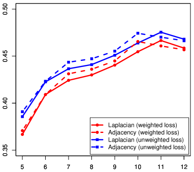
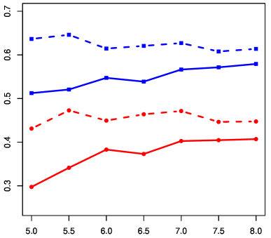
Figure 1: Comparison of Mixed-SCORE-Laplacian (solid curves) and orthodox Mixed-SCORE (dashed curves). In both panels, the $x$-axis is $\|\theta\|$, and the $y$-axis is either the unweighted $\ell^{1}$-loss ${\cal L}(\hat{\Pi},\Pi)$ (blue curves) or the weighted $\ell^{1}$-loss ${\cal L}^{w}(\hat{\Pi},\Pi)$ (red curves), averaged over 100 repetitions. The left panel corresponds to moderate degree heterogeneity, where $\theta_{i}$’s are drawn from a uniform distribution. The right panel corresponds to severe degree heterogeneity, where $\theta_{i}$’s are drawn from a Pareto distribution. $(n,K)=(2000,2)$.

Experiment 1: Comparison with the orthodox Mixed-SCORE

We compare the numerical performances of Mixed-SCORE-Laplacian (MSL) and orthodox Mixed-SCORE (OMS) Jin et al. (2017). A major difference between two methods is that OMS uses $M=I_{n}$ in (1.7), while our proposed MSL uses $M=[\mathrm{diag}(d_{1},\ldots,d_{n})+\bar{d}I_{n}]^{-1/2}$. Fix $(n,K)=(2000,2)$. We consider two sub-experiments: In Experiment 1.1, the fixed distribution $F$ is $\mathrm{Uniform}([0.3,5])$; in Experiment 1.2, $F$ is $\mathrm{Pareto}(10,0.3)$. We let $b_{n}=\|\theta\|$ range in $\{5,6,\ldots,12\}$ in Experiment 1.1 and range in $\{5,5.5,6,6.5,\ldots,8\}$ in Experiment 1.2. As $b_{n}$ varies, we change $\beta_{n}$ accordingly by fixing $\mathrm{SNR}=b_{n}\cdot\beta_{n}=4.5$. We report both the unweighted $\ell^{1}$-loss $\mathcal{L}(\hat{\Pi},\Pi)$ and the weighted $\ell^{1}$-loss $\mathcal{L}^{w}(\hat{\Pi},\Pi)$, over 100 repetitions. The results are displayed in Figure 1.

We first look at the unweighted $\ell^{1}$-loss (blue curves). When degree heterogeneity is moderate (left panel of Figure 1), MSL and OMS have similar performances. This is as expected, because both methods can attain the optimal rate under moderate degree heterogeneity. When degree heterogeneity is severe (right panel of Figure 1), MSL significantly outperforms OMS. This is consistent with our theory, where the rate of MLS is optimal in this case but the rate of OMS is non-optimal. These numerical results also confirm the advantage of using a pre-PCA normalization. We then look at the weighted $\ell^{1}$-loss (red curves), where the conclusions are similar. Note that for each method, the magnitudes of two loss metrics are close under moderate degree heterogeneity (left panel) and quite different under severe degree heterogeneity (right panel). This is also consistent with the definitions of two loss metrics.

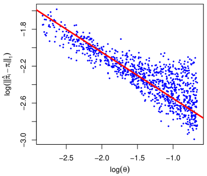
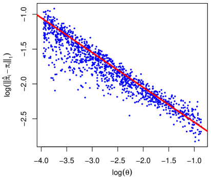
Figure 2: $\theta_{i}$’s are generated from $\mathcal{U}([0.3,5])$ and Pareto$(10,0.3)$, respectively for the left and the right. In both plots, the slope of the red lines is $-1/2$. The results are based on $100$ repetitions.

Experiment 2: Node-wise errors of Mixed-SCORE-Laplacian

We investigate the errors of Mixed-SCORE-Laplacian at individual $\hat{\pi}_{i}$’s and study its relationship with $\theta_{i}$. Theorem 3.2 claims that the error at $\hat{\pi}_{i}$ is approximately proportional to $(\theta_{i}\wedge\bar{\theta})^{-1/2}$. To verify this result, we plot $\log(\|\hat{\pi}_{i}-\pi_{i}\|_{1})$ versus $\log(\theta_{i})$, for $\theta_{i}\leq\bar{\theta}$. We expect the scatter plot to fit a straight light with a slope of $-1/2$. Fix $(n,K)=(2000,2)$. We first generate $\theta$ and $\Pi$ as in Experiment 1. We then fix $(\theta,\Pi)$, generate 100 networks, and compute the average of $\|\hat{\pi}_{i}-\pi_{i}\|_{1}$ over these 100 repetitions, for each $1\leq i\leq n$. Similarly as in Experiment 1, we consider two experiments: In Experiment 2.1, the fixed distribution $F$ is $\mathrm{Uniform}([0.3,5])$; in Experiment 2.2, $F$ is $\mathrm{Pareto}(10,0.3)$. We fix $b_{n}=\|\theta\|=26$ and $\mathrm{SNR}=b_{n}\cdot\beta_{n}=23$. The results are displayed in Figure 2. For both moderate degree heterogeneity (left panel) and severe degree heterogeneity (right panel), the plot fits reasonably well a straight line with slope $-1/2$. This verifies the claim of Theorem 3.2. Interestingly,when degree heterogeneity is more severe, the empirical evidence of Theorem 3.2 is even stronger.

7 Discussions

Many real networks have severe degree heterogeneity. It motivates the study of network models equipped with node-wise degree parameters. When the target quantity is the underlying community structure, the large number of degree parameters are nuisance. There was little understanding to how these nuisance parameters affect the inference of community structure. We give a rigorous answer in the context of mixed membership estimation. Under the DCMM model, we show that the $n$ degree parameters $\theta_{1},\theta_{2},\ldots,\theta_{n}$ affect the optimal rate of mixed membership estimation through $\bar{\theta}$ and $F_{n}(\cdot)$, where $\bar{\theta}$ captures the overall sparsity and $F_{n}(\cdot)$ captures the degree heterogeneity. We identify both examples where the degree heterogeneity does or does not alter the optimal rate.

A desirable mixed membership estimation method should be optimally adaptive to degree heterogeneity. The OMS Jin et al. (2017) is a spectral algorithm. It attains the optimal rate under moderate degree heterogeneity but not severe degree heterogeneity. We combine OMS with a pre-PCA normalization by the regularized graph Laplacian, and show that the new algorithm achieves the optimal rate under quite arbitrary degree heterogeneity. On the one hand, it is surprising that such a simple variant of OMS can be optimally adaptive. On the other hand, it requires a lot of non-trivial insights and analysis to come to this conclusion: (a) We first derive the optimal rate, so that we have a benchmark to access the optimality of any method. (b) We point out that a pre-PCA normalization like (1.7) is promising to tackle severe degree heterogeneity. (c) We calculate the entry-wise SNRs of empirical eigenvectors and find out that $M\propto\Theta^{-1/2}$ is the ideal choice, which motivates the use of graph Laplacian. (d) With many technical efforts (especially the large-deviation analysis of eigenvectors in Section 4), we rigorously prove that the resulting spectral algorithm is optimally adaptive. Our contribution is far more than a naive combination of OMS and graph Laplacian. Without our insights and analysis, it was even unclear whether there exists an $M$ that is optimal, not to say whether graph Laplacian is the optimal $M$.

As a byproduct of our analysis, we provide a new row-wise large-deviation bound for the leading eigenvectors of the regularized graph Laplacian. Most existing results of entrywise eigenvector analysis (e.g., Abbe et al. (2020)) focus on the case of no degree heterogeneity or moderate degree heterogeneity, and study the adjacency matrix. We provide the first entrywise eigenvector analysis that simultaneously (i) deals with graph Laplacian, (ii) allows for severe degree heterogeneity, and (iii) yields the $\theta_{i}$-dependent bound for each entry. We believe this result is of independent interest.

Appendix A Proof of Lemma 2.1

Recall that $L_{0}=H_{0}^{-\frac{1}{2}}\Theta\Pi(P\Pi^{\prime}\Theta H_{0}^{-\frac{1}{2}})$. Under the condition that each community has at least one pure node, $L_{0}$ has a rank $K$. It follows that $L_{0}$ has the same column space as $H_{0}^{-\frac{1}{2}}\Theta\Pi$. Meanwhile, $\Xi=[\xi_{1},\xi_{2},\ldots,\xi_{K}]$ also has the same column space as $L_{0}$. Therefore, there exists a non-singular matrix $B\in\mathbb{R}^{K\times K}$ such that

$$\Xi=H_{0}^{-\frac{1}{2}}\Theta\Pi B.$$

Write $B=[b_{1},b_{2},\ldots,b_{K}]$. Define $v_{1},v_{2},\ldots,v_{K}\in\mathbb{R}^{K-1}$ by $v_{k}(\ell)=b_{\ell+1}(k)/b_{1}(k)$, for $1\leq k\leq K$, $1\leq\ell\leq K-1$. Write $V=[v_{1},v_{2},\ldots,v_{K}]^{\prime}\in\mathbb{R}^{K\times(K-1)}$. It follows that

$$B=\mathrm{diag}(b_{1})[{\bf 1}_{K},V].$$

By definition of $R$, $[{\bf 1}_{n},R]=[\mathrm{diag}(\xi_{1})]^{-1}\Xi$. It follows that

$$[{\bf 1}_{n},R] =[\mathrm{diag}(\xi_{1})]^{-1}\Xi=[\mathrm{diag}(\xi_{1})]^{-1}H_{0}^{-\frac{1}{2}}\Theta\Pi B$$

$$=[\mathrm{diag}(\xi_{1})]^{-1}H_{0}^{-\frac{1}{2}}\Theta\Pi\mathrm{diag}(b_{1})[{\bf 1}_{K},V].$$

Define $W=[\mathrm{diag}(\xi_{1})]^{-1}H_{0}^{-\frac{1}{2}}\Theta\Pi\mathrm{diag}(b_{1})$. The above equation implies that ${\bf 1}_{n}=W{\bf 1}_{K}$ and $R=WV$. Denote by $w_{i}^{\prime}$ the $i$th row of $V$. It follows that $w_{i}^{\prime}{\bf 1}_{K}=1$ and $r_{i}=\sum_{k=1}^{K}w_{i}(k)v_{k}$. Furthermore, under the condition (3.3), we can show that both $\xi_{1}$ and $b_{1}$ are strictly positive vectors; the proof is similar to the proof of Lemma B.4 of Jin et al. (2017), which we omit. It suggests that $W$ is also a nonnegative matrix. Combining the above, each $r_{i}$ is a convex combination of $v_{1},v_{2},\ldots,v_{K}$. This proves the simplex structure.

We now derive the connection between $w_{i}$ and $\pi_{i}$. Write $\alpha_{i}=\xi_{1}^{-1}(i)H^{-\frac{1}{2}}_{0}(i,i)\theta_{i}$. Then, $w^{\prime}_{i}=\alpha_{i}\cdot\pi_{i}^{\prime}\mathrm{diag}(b_{1})=\alpha_{i}\cdot(\pi_{i}\circ b_{1})$. Since $\|w_{i}\|_{1}=1$, we immediately have $\alpha_{i}=1/\|\pi_{i}\circ b_{1}\|_{1}$. This proves that $w_{i}=\frac{1}{\|\pi_{i}\circ b_{1}\|_{1}}(\pi_{i}\circ b_{1})$. To get the expression of $B_{1}$, we notice that

$$\Lambda =\Xi^{\prime}L_{0}\Xi=(H_{0}^{-\frac{1}{2}}\Theta\Pi B)^{\prime}(H_{0}^{-\frac{1}{2}}\Theta\Pi P\Pi^{\prime}\Theta H_{0}^{-\frac{1}{2}})(H_{0}^{-\frac{1}{2}}\Theta\Pi B)$$

$$=B^{\prime}(\Pi^{\prime}\Theta D_{\theta}^{-1}\Theta\Pi)P(\Pi^{\prime}\Theta D_{\theta}^{-1}\Theta\Pi)B^{\prime}=K^{-2}\cdot B^{\prime}GPGB,$$

where $D_{\theta}$ and $G$ are as defined in Section 3 and we note that $D_{\theta}$ is actually $H_{0}$. Moreover, $G=K\cdot(H_{0}^{-\frac{1}{2}}\Theta\Pi)^{\prime}(H_{0}^{-\frac{1}{2}}\Theta\Pi)=K\cdot(\Xi B^{-1})^{\prime}(\Xi B^{-1})=K\cdot(BB^{\prime})^{-1}$. It follows that

$$B\Lambda B^{\prime}=K^{-2}\cdot BB^{\prime}GPGBB=P.$$

Write $\Lambda=\mathrm{diag}(\lambda_{1},\Lambda_{1})$, where $\Lambda_{1}=\mathrm{diag}(\lambda_{2},\ldots,\lambda_{K})$. Also, recall that $B=\mathrm{diag}(b_{1})[{\bf 1}_{K},V]$. We plug them into the above expression to get

$$P=\mathrm{diag}(b_{1})[{\bf 1}_{K},V]\begin{bmatrix}\lambda_{1}\\ &\Lambda_{1}\end{bmatrix}\begin{bmatrix}{\bf 1}_{K}^{\prime}\\ V^{\prime}\end{bmatrix}\mathrm{diag}(b_{1}).$$

It follows that $P(k,k)=b_{1}(k)\cdot[\lambda_{1}+v_{k}^{\prime}\Lambda_{1}v_{k}]\cdot b_{1}(k)$. The identifiability condition (1.3) says that $P(k,k)=1$. Therefore, $b_{1}(k)=1/\sqrt{\lambda_{1}+v_{k}^{\prime}\Lambda_{1}v_{k}}$.

Appendix B Auxiliary lemmas on regularized graph Laplacian

Denote

$$S_{1}=\{1\leq i\leq n:\theta_{i}\geq\bar{\theta}\},\qquad S_{2}=\{1\leq i\leq n:\theta_{i}<\bar{\theta}\}.$$ (B.1)

B.1 Properties of $L_{0}$

Recall that $L_{0}=H_{0}^{-\frac{1}{2}}\Omega H_{0}^{-\frac{1}{2}}$. We state the following three lemmas on its spectrum properties and also estimates of the degree regularization matrix $H_{0}$.

Lemma B.1.

Under the conditions of Theorem 3.1,

$$\lambda_{1}>0,\quad\lambda_{1}\asymp K^{-1}\lambda_{1}(PG),\quad|\lambda_{K}|\asymp K^{-1}\lambda_{K}(PG),\quad\lambda_{1}-\max_{2\leq k\leq K}|\lambda_{k}|\geq c\lambda_{1}.$$ (B.2)

Lemma B.2.

Under the conditions of Theorem 3.1,

$$\xi_{1}(i)\asymp\frac{1}{\sqrt{n}}\begin{cases}\sqrt{\theta_{i}/\bar{\theta}},&i\in S_{1},\\ \theta_{i}/\bar{\theta},&i\in S_{2},\end{cases}\qquad\|\Xi(i)\|\leq\frac{C\sqrt{K}}{\sqrt{n}}\begin{cases}\sqrt{\theta_{i}/\bar{\theta}},&i\in S_{1},\\ \theta_{i}/\bar{\theta},&i\in S_{2},\end{cases}$$ (B.3)

and

$$H_{0}(i,i)\asymp\begin{cases}n\theta_{i}\bar{\theta},&i\in S_{1},\\ n\bar{\theta}^{2},&i\in S_{2}.\end{cases}$$ (B.4)

Lemma B.3.

Under the conditions of Theorem 3.1, with probability $1-o(n^{-3})$,

$$\|I_{n}-H_{0}^{-1}H\|\leq\frac{C\sqrt{\log(n)}}{\sqrt{n\bar{\theta}^{2}}},\qquad\|H_{0}^{-1/2}(A-\Omega)H_{0}^{-1/2}\|\leq\frac{C}{\sqrt{n\bar{\theta}^{2}}}.$$ (B.5)

The proof of Lemma B.1 is straightforward by noting that $D_{\theta}=H_{0}^{-1}$ (see the definition of $D_{\theta}$ in Section 3) and therefore $L_{0}$ share the same eigenvalues as $K^{-1}PG$. Immediately, one can conclude (B.2) from (3.2). In the sequel, we show the proof of the Lemmas B.2 and B.3. Before that, we introduce the Bernstein inequality which we will use frequently to bound sum of independent Bernoulli entries.

Theorem B.1 (Bernstein inequality).

Let $X_{1},\cdots,X_{n}$ be independent zero-mean random variables. Suppose that $|X_{i}|\leq M$ almost surely, for all $i$. Then for all positive $t$,

$$\mathbb{P}\Big{(}\Big{|}\sum_{i=1}^{n}X_{i}\Big{|}\geq t\Big{)}\leq 2\exp\Big{(}-\frac{t^{2}/2}{\sigma^{2}+Mt/3}\Big{)},$$

with $\sigma^{2}:=\sum_{i=1}^{n}\mathbb{E}(X_{i}^{2})$. In particular, taking $t=C(\sigma\sqrt{\log(n)}+M\log(n))$ for properly large $C$, then

$$\Big{|}\sum_{i=1}^{n}X_{i}\Big{|}\leq C(\sigma\sqrt{\log(n)}+M\log(n))\quad\text{ with probability $1-o(n^{-5})$}.$$

Proof of Lemma B.2.

First, we show (B.4). Uniformly for all $1\leq i\leq n$,

$$\mathbb{E}d_{i}=\theta_{i}\sum_{j\neq i}\theta_{j}\pi_{j}^{\prime}P\pi_{i}\geq\theta_{i}\sum_{j\neq i}\theta_{j}\sum_{k}\pi_{j}(k)\pi_{i}(k)\geq c_{1}n\theta_{i}\bar{\theta}$$ (B.6)

by the last inequality in (3.1). On the other hand, $\pi_{j}^{\prime}P\pi_{i}\leq\max_{t,s}P(t,s)$ for all $i,j$, then $\mathbb{E}d_{i}=\theta_{i}\sum_{j\neq i}\theta_{j}\pi_{j}^{\prime}P\pi_{i}\leq cn\theta_{i}\bar{\theta}$ for all $i$. As a result, $\mathbb{E}d_{i}\asymp n\theta_{i}\bar{\theta}$, $\mathbb{E}\bar{d}\asymp n\bar{\theta}^{2}$; and further

$$H_{0}(i,i)=\mathbb{E}d_{i}+\mathbb{E}\bar{d}\asymp\begin{cases}n\theta_{i}\bar{\theta},&i\in S_{1},\\ n\bar{\theta}^{2},&i\in S_{2}.\end{cases}$$

This completes the proof of (B.4). Next, we turn to prove (B.3). By the definition $L_{0}=H_{0}^{-\frac{1}{2}}\Omega H_{0}^{-\frac{1}{2}}$, there exists a non-singular matrix $B\in\mathbb{R}^{K\times K}$ satisfying

$$\Xi=H_{0}^{-\frac{1}{2}}\Theta\Pi B,\qquad BB^{\prime}=(\Pi^{\prime}\Theta H_{0}^{-1}\Theta\Pi)^{-1}.$$

Using (3.1) and $H_{0}=D_{\theta}$, one gets $\|BB^{\prime}\|\leq Kc$, $\lambda_{\min}(BB^{\prime})\geq Kc^{-1}$. Write $B=({b}_{1},\cdots,{b}_{K})$. We have $Kc^{-1}\leq\|b_{i}\|^{2}\leq Kc$ for $1\leq i\leq K$. Taking the $i$-th row of $\Xi$,

$$\|\Xi(i)\|=\frac{\theta_{i}}{\sqrt{H_{0}(i,i)}}\|\pi_{i}^{\prime}B\|\leq C\sqrt{\frac{\theta_{i}}{n\bar{\theta}}}\|\pi_{i}\|\|BB^{\prime}\|^{\frac{1}{2}}\leq C\sqrt{K}\,\sqrt{\frac{\theta_{i}}{n\bar{\theta}}}.$$

For the leading eigenvector $\xi_{1}$, we have

$$\xi_{1}(i)=\frac{\theta_{i}}{\sqrt{H_{0}(i,i)}}\pi_{i}^{\prime}b_{1}$$

It follows from $L_{0}\Xi=\Xi\Lambda$ that $H_{0}^{-\frac{1}{2}}\Theta\Pi P\Pi^{\prime}\Theta H_{0}^{-1}\Theta\Pi B=H_{0}^{-\frac{1}{2}}\Theta\Pi B\Lambda$, which implies that $P\Pi^{\prime}\Theta H_{0}^{-1}\Theta\Pi B=B\Lambda$. As a consequence, $b_{1}$ is the first right singular vector of $P\Pi^{\prime}\Theta H_{0}^{-1}\Theta\Pi$, and equivalently, the first right singular vector of $PG$. Using (3.3), we easily conclude that $b_{1}(k)>0,b_{1}(k)\asymp 1$ for all $1\leq k\leq K$. Then, $\pi_{i}^{\prime}b_{1}\asymp 1$ for all $1\leq i\leq n$, and the entrywise estimate of $\xi_{1}$ simply follows from (B.4). ∎

Proof of Lemma B.3.

Recall the definition of $H_{0},H$. We write

$$\frac{H(i,i)}{H_{0}(i,i)}-1=\frac{d_{i}-\mathbb{E}d_{i}+\bar{d}-\mathbb{E}\bar{d}}{H_{0}(i,i)},\qquad d_{i}-\mathbb{E}d_{i}=\sum_{j\neq i}A_{ij}-\mathbb{E}A_{ij}.$$

By (B.4), we easily see that $H_{0}(i,i)\asymp n\bar{\theta}(\theta_{i}\vee\bar{\theta})$. What remains is to estimate the numerator, or $d_{i}-\mathbb{E}d_{i}$ for all $1\leq i\leq n$. This actually can be done with the help of Bernstein inequality. Applying the Bernstein inequality (Theorem B.1) to $d_{i}-\mathbb{E}d_{i}$, we see that

$$\mathbf{P}\Big{(}\big{|}\sum_{j\neq i}A_{ij}-\mathbb{E}A_{ij}\big{|}\geq t\Big{)}\leq 2\exp\bigg{(}{-\frac{\frac{1}{2}t^{2}}{\sum_{j\neq i}{\rm var}A_{ij}+\frac{1}{3}Mt}}\bigg{)}$$

where $M=\sup_{j}|A_{ij}-\mathbb{E}A_{ij}|\leq 2$. Moreover, we have the crude bound

$$\sum_{j\neq i}{\rm var}A_{ij}\leq cn\theta_{i}\bar{\theta}.$$

Taking $t=C\sqrt{\log(n)}\sqrt{n\bar{\theta}\theta_{i}\vee\log(n)}$, it gives that $\big{|}\sum_{j\neq i}A_{ij}-\mathbb{E}A_{ij}\big{|}\leq C\sqrt{\log(n)(n\bar{\theta}\theta_{i}\vee\log(n))}$ with probability $1-o(n^{-5})$. Consider all $i$’s together, one gets

$$\mathbf{P}\Big{(}\bigcup_{i=1}^{n}\Big{\{}\big{|}\sum_{j\neq i}A_{ij}-\mathbb{E}A_{ij}\big{|}\geq C\sqrt{\log n}\,\big{(}\sqrt{n\theta_{i}\bar{\theta}}\vee\sqrt{\log n}\big{)}\,\Big{\}}\Big{)}\leq cn^{-4},$$

This, combined with $H_{0}(i,i)\asymp n\bar{\theta}(\theta_{i}\vee\bar{\theta})$, implies that

$$\Big{|}1-H(i,i)/H_{0}(i,i)\Big{|} \leq\frac{|d_{i}-\mathbb{E}d_{i}|}{H_{0}(i,i)}+\frac{1}{n}\sum_{j=1}^{n}\frac{|d_{j}-\mathbb{E}d_{j}|}{H_{0}(i,i)}$$

$$\leq C\sqrt{\frac{\log n}{n\bar{\theta}^{2}}}+C\sqrt{\frac{\log n}{n\bar{\theta}^{2}}}\frac{1}{n}\sum_{j=1}^{n}\max\Big{\{}\sqrt{\frac{\theta_{j}}{\bar{\theta}}},\sqrt{\frac{\log n}{n\bar{\theta}^{2}}}\,\Big{\}}$$

$$\leq C\sqrt{\frac{\log n}{n\bar{\theta}^{2}}}\Big{(}1+\frac{1}{n}\sum_{j=1}^{n}\sqrt{\frac{\theta_{j}}{\bar{\theta}}}+\sqrt{\frac{\log n}{n\bar{\theta}^{2}}}\,\Big{)}\leq C\sqrt{\frac{\log n}{n\bar{\theta}^{2}}}$$

with probability $1-o(n^{-3})$ uniformly for all $1\leq i\leq n$. Here in the last step, we used the Cauchy-Schwarz inequality $\sum_{j=1}^{n}\sqrt{\theta_{j}}\leq\sqrt{n}\sqrt{\sum_{j=1}^{n}\theta_{j}}=n\sqrt{\bar{\theta}}$. This finished the first estimate of (B.5). Now, we proceed to the second estimate. We crudely bound $\|H_{0}^{-1/2}(A-\Omega)H_{0}^{-1/2}\|$ by $\|H_{0}^{-1/2}WH_{0}^{-1/2}\|+\|H_{0}^{-1/2}{\rm diag}(\Omega)H_{0}^{-1/2}\|$. First it is easy to get the bound

$$\|H_{0}^{-1/2}{\rm diag}(\Omega)H_{0}^{-1/2}\|\leq C\max_{1\leq i\leq n}\frac{\theta_{i}^{2}\pi_{i}^{\prime}P\pi_{i}}{H_{0}(i,i)}\leq\frac{C}{n\bar{\theta}}\leq\frac{C}{\sqrt{n\bar{\theta}^{2}}}.$$

Next, we apply the non-asymptotic bounds for random matrices in Bandeira and Van Handel (2016) to bound the operator norm of $\widehat{W}:=H_{0}^{-1/2}WH_{0}^{-1/2}$. Note that $\widehat{W}$ is a symmetric random matrix with independent upper triangular entries. Using Corollary 3.12 of Bandeira and Van Handel (2016) with Remark 3.13, we bound

$$\mathbb{P}(\|\widehat{W}\|\geq C\tilde{\sigma}+t)\leq ne^{-t^{2}/c\tilde{\sigma}_{*}^{2}}$$

for some constant $C,c>0$, with

$$\tilde{\sigma}=\max_{i}\sqrt{\sum_{j}\mathbb{E}\widehat{W}(i,j)^{2}}\leq 1/\sqrt{n\bar{\theta}^{2}},\quad\tilde{\sigma}_{*}=\max_{i,j}\|\widehat{W}(i,j)\|_{\infty}\leq C/n\bar{\theta}^{2}.$$

Then one just need to take $t=c/\sqrt{n\bar{\theta}^{2}}$ for properly large $c$ and use the assumption $n\bar{\theta}^{2}\gg\log(n)$. It follows that $\|\widehat{W}\|\leq C/\sqrt{n\bar{\theta}^{2}}$ with probability $1-o(n^{-3})$. We thus complete the proof of Lemma B.3. ∎

B.2 Properties of $\tilde{L}^{(i)}$

In this section, for an arbitrary fixed index $i$ and the intermediate matrix $\tilde{L}^{(i)}$, we collect the spectrum properties of $\tilde{L}^{(i)}$ and estimate on $\tilde{H}^{(i)}$ in the lemmas below. Let $E$ be the event that Lemma B.3 holds.

Lemma B.4.

Under the conditions in Theorem 3.1. Over the event $E$, for any fixed $1\leq i\leq n$, the eigenvalues $\tilde{\lambda}^{(i)}_{1},\cdots,\tilde{\lambda}^{(i)}_{K}$ of $\tilde{L}^{(i)}$ satisfy

$$\tilde{\lambda}^{(i)}_{1}>0,\quad\tilde{\lambda}^{(i)}_{1}\asymp K^{-1}\lambda_{1}(PG),\quad|\tilde{\lambda}^{(i)}_{K}|\asymp K^{-1}|\lambda_{K}(PG)|,\quad\tilde{\lambda}^{(i)}_{1}-\max_{2\leq k\leq K}|\tilde{\lambda}^{(i)}_{k}|\geq C^{-1}\tilde{\lambda}^{(i)}_{1};$$ (B.7)

and for the associated eigenvectors,

$$\tilde{\xi}^{(i)}_{1}(j)\asymp\frac{1}{\sqrt{n}}\begin{cases}\sqrt{\theta_{j}/\bar{\theta}},&j\in S_{1},\\ \theta_{j}/\bar{\theta},&j\in S_{2},\end{cases}\qquad\|\tilde{\Xi}^{(i)}(j)\|\leq\frac{C\sqrt{K}}{\sqrt{n}}\begin{cases}\sqrt{\theta_{j}/\bar{\theta}},&j\in S_{1},\\ \theta_{j}/\bar{\theta},&j\in S_{2}.\end{cases}$$ (B.8)

Lemma B.5.

Under the conditions of Theorem 3.1. Over the event $E$, for any fixed $1\leq i\leq n$ and $\tilde{H}^{(i)}$,

$$\|I_{n}-H_{0}^{-1}\tilde{H}^{(i)}\|\leq\frac{C\sqrt{\log(n)}}{\sqrt{n\bar{\theta}^{2}}},\quad\|I_{n}-(\tilde{H}^{(i)})^{-1}{H}\|\leq\frac{C\sqrt{\log(n)}}{\sqrt{n\bar{\theta}^{2}}}.$$ (B.9)

Besides the above lemma, by Theorem B.1 and after elementary computations, we also have that for each $1\leq j\leq n,j\neq i$, over the event $E$,

$$\big{|}\tilde{H}^{(i)}(j,j)-H(j,j)\big{|} =\Big{|}-A(j,i)-\frac{1}{n}\Big{(}\sum_{s\neq i}A(i,s)+\sum_{s\neq i}A(i,s)-\mathbb{E}A(i,s)\Big{)}\Big{|}$$

$$\leq A(j,i)+C\theta_{i}\bar{\theta}+\frac{C\log(n)}{n};$$ (B.10)

and

$$\big{|}\tilde{H}^{(i)}(i,i)-H(i,i)\big{|}\leq C\sqrt{n\theta_{i}\bar{\theta}\log n}+C\log(n).$$ (B.11)

Applying (B.2) and (B.11) with Lemma B.3, it is easy to deduce the estimates in Lemma B.5. To show the eigen-properties of $\tilde{L}$ in Lemma B.4, one only need to rely on the estimate

$$\|\tilde{L}^{(i)}-L\|\asymp\|I_{n}-H_{0}^{-1}\tilde{H}^{(i)}\|\lambda_{1}(L_{0})\leq C\sqrt{\frac{\log(n)}{n\bar{\theta}^{2}}}\gg|\lambda_{K}|$$

under the assumption of Theorem 3.1, then (B.7) can be derived simply by further applying Lemma B.1. Moreover, (B.8) follows from Lemmas 4.1, C.1 and B.2. Thereby, we omit the proofs of Lemmas B.4 and B.5. We comment here that the proof of Lemmas 4.1, C.1 only depends on the lemmas in Section B.1, i.e., the properties of $L_{0}$, not the properties of $\tilde{L}^{(i)}$. There is no circular logic for the lemmas presenting in this subsection.

Appendix C Entrywise eigenvector analysis

Here we show the complete proof of Theorem 3.1 and a brief proof of Corollary 3.1 in our manuscript. In Sections C.1 -C.3, we state the proofs of key lemmas for proving (3.6), while the claim of (3.6) is already presented in the manuscript. Section C.4 collects the proof of the second claim in Theorem 3.1 (i.e., (3.7)) which provides the entry-wise estimates for the $2$- to $K$-th eigenvectors. Similarly to the proof of the first claim in Theorem 3.1 (i.e., (3.6) ), we introduce three key lemmas, Lemmas C.1- C.3, counterpart to Lemmas 4.1-4.3. The proofs of Lemmas C.1- C.3 are provided correspondingly in Section C.5-C.7. In the end of this section, we briefly state the proof of Corollary 3.1 based on Theorem 3.1.

C.1 Proof of Lemma 4.1

In this subsection, we show the proof of Lemma 4.1 using the eigen-properties of $L_{0}$ in Section B.1.

Fix the index $i$, we study the perturbation from $L_{0}=H_{0}^{-1/2}\Omega H_{0}^{-1/2}$ to $\tilde{L}^{(i)}=(\tilde{H}^{(i)})^{-1/2}\Omega(\tilde{H}^{(i)})^{-1/2}$. By definition,

$$L_{0}=H_{0}^{-1/2}\Omega H_{0}^{-1/2}=\sum_{k=1}^{K}\lambda_{k}\xi_{k}\xi_{k}^{\prime},\qquad(\tilde{H}^{(i)})^{-1/2}\Omega(\tilde{H}^{(i)})^{-1/2}\tilde{\xi}^{(i)}_{1}=\tilde{\lambda}^{(i)}_{1}\tilde{\xi}^{(i)}_{1}.$$

Write $\tilde{Y}\equiv\tilde{Y}^{(i)}:={H_{0}^{1/2}(\tilde{H}^{(i)})^{-1/2}}$. Then, we have

$$\tilde{Y}\bigl{(}\sum_{k=1}^{K}\lambda_{k}\xi_{k}\xi_{k}^{\prime}\bigr{)}\tilde{Y}\tilde{\xi}^{(i)}_{1}=\tilde{\lambda}^{(i)}_{1}\tilde{\xi}^{(i)}_{1}.$$

It follows that, for each $1\leq j\leq n$,

$$\frac{1}{\tilde{Y}(j,j)}\tilde{\xi}^{(i)}_{1}(j)=\frac{\lambda_{1}(\xi_{1}^{\prime}\tilde{Y}\tilde{\xi}^{(i)}_{1})}{\tilde{\lambda}^{(i)}_{1}}\xi_{1}(j)+\sum_{k=2}^{K}\frac{\lambda_{k}(\xi_{k}^{\prime}\tilde{Y}\tilde{\xi}^{(i)}_{1})}{\tilde{\lambda}^{(i)}_{1}}\xi_{k}(j).$$ (C.1)

As a result,

$$|\tilde{\xi}^{(i)}_{1}(j)-\xi_{1}(j)|\leq\Bigl{|}\frac{1}{\tilde{Y}(j,j)}-1\Bigr{|}|\tilde{\xi}^{(i)}_{1}(j)|+\Bigl{|}\frac{\lambda_{1}(\xi_{1}^{\prime}\tilde{Y}\tilde{\xi}^{(i)}_{1})}{\tilde{\lambda}^{(i)}_{1}}-1\Bigr{|}|\xi_{1}(j)|+\sum_{k=2}^{K}\Bigl{|}\frac{\lambda_{k}(\xi_{k}^{\prime}\tilde{Y}\tilde{\xi}^{(i)}_{1})}{\tilde{\lambda}^{(i)}_{1}}\Bigr{|}|\xi_{k}(j)|.$$ (C.2)

By Lemma B.1, $\|L_{0}\|\leq CK^{-1}\lambda_{1}(PG)$. And using the first estimate in (B.9), it is easy to conclude that

$$\|\tilde{Y}-I_{n}\|=\big{\|}I_{n}-(H_{0}^{-1}\tilde{H}^{(i)})^{-\frac{1}{2}}\big{\|}\leq\frac{C\sqrt{\log(n)}}{\sqrt{n\bar{\theta}^{2}}},$$ (C.3)

over the event $E$ where Lemma B.3 holds. As a result, we have $\|\tilde{L}^{(i)}-L_{0}\|\leq CK^{-1}\lambda_{1}(PG)\|\tilde{Y}-I_{n}\|$. Using Weyl’s inequality, we then see that

$$\max_{1\leq k\leq K}{|\tilde{\lambda}^{(i)}_{k}-\lambda_{k}|} \leq\|\tilde{L}^{(i)}-L_{0}\|\leq CK^{-1}\lambda_{1}(PG)\|\tilde{Y}-I_{n}\|\leq C\|\tilde{Y}-I_{n}\|$$

since $\lambda_{1}(PG)\leq CK$ under our model assumption. Furthermore, by Lemma B.1, the eigen-gap between the largest eigenvalue and the other nonzero eigenvalues of $L_{0}$ is at the order $K^{-1}\lambda_{1}(PG)$. Hence, the eigengap between $\lambda_{1}$ and $\tilde{\lambda}_{2}^{(i)},\cdots,\tilde{\lambda}_{K}^{(i)}$ is still of the order $K^{-1}\lambda_{1}(PG)$. It follows from the sin-theta theorem that

$$|\xi_{1}^{\prime}\tilde{Y}\tilde{\xi}^{(i)}_{1}-1| \leq|\xi_{1}^{\prime}\tilde{\xi}^{(i)}_{1}-1|+\|\xi_{1}^{\prime}(\tilde{Y}-I_{n})\tilde{\xi}^{(i)}_{1}\|$$

$$\leq C(K\lambda_{1}^{-1}(PG)\|\tilde{L}^{(i)}-L_{0}\|)^{2}+\|\tilde{Y}-I_{n}\|\leq C\|\tilde{Y}-I_{n}\|.$$

Here ${\rm sgn}(\xi_{1}^{\prime}\tilde{\xi}^{(i)}_{1})=1$ since we fix our choices of $\xi_{1},\tilde{\xi}^{(i)}_{1}$ with positive first components and they are both from the positive matrices. Then this will be claimed by Perron’s theorem.

Using Cauchy-Schwarz inequality, we bound $\sum_{k=2}^{K}|\xi_{k}^{\prime}\tilde{Y}\tilde{\xi}^{(i)}_{1}||\xi_{k}(j)|\leq\|\Xi_{1}^{\prime}\tilde{Y}\tilde{\xi}^{(i)}_{1}\|\|\Xi_{1}(j)\|$. And by sine-theta theorem,

$$\|\Xi_{1}^{\prime}\tilde{Y}\tilde{\xi}^{(i)}_{1}\| \leq\|(\tilde{\xi}^{(i)}_{1})^{\prime}\Xi_{1}\|+\|\tilde{Y}-I_{n}\|$$

$$\leq C\Big{(}K\lambda_{1}^{-1}(PG)\|\tilde{L}^{(i)}-L_{0}\|+\|\tilde{Y}-I_{n}\|\Big{)}$$

$$\leq C\|\tilde{Y}-I_{n}\|.$$

Plugging the above estimates, we have

$$|\tilde{\xi}^{(i)}_{1}(j)-\xi_{1}(j)| \leq C\|\tilde{Y}-I_{n}\||\tilde{\xi}^{(i)}_{1}(j)|+C\|\tilde{Y}-I_{n}\|\|\Xi(j)\|$$

$$\leq C\|\tilde{Y}-I_{n}\||\tilde{\xi}^{(i)}_{1}(j)-\xi_{1}(j)|+C\|\tilde{Y}-I_{n}\|\|\Xi(j)\|.$$

Since $\|\tilde{Y}-I_{n}\|=o(1)$ over the event $E$, rearranging the terms gives

$$|\tilde{\xi}^{(i)}_{1}(j)-\xi_{1}(j)|\leq C\|\tilde{Y}-I_{n}\|\|\Xi(j)\|,\qquad\mbox{for all }1\leq t\leq n.$$ (C.4)

We plug (C.3) into (C.4) and use the bound for $\|\Xi(j)\|$ in (B.3). It follows that over the event $E$, for all $1\leq j\leq n$,

$$|\tilde{\xi}^{(i)}_{1}(j)-\xi_{1}(j)|\leq C\sqrt{K}\sqrt{\frac{\log(n)}{n\bar{\theta}^{2}}}\sqrt{\frac{\theta_{j}}{n\bar{\theta}}}\bigg{(}\sqrt{\frac{\theta_{j}}{\bar{\theta}}}\wedge 1\,\bigg{)}$$ (C.5)

Then, consider all $i$’s together, we conclude (4.3) with probability $1-o(n^{-3})$ simultaneously for all $1\leq i,j\leq n$.

C.2 Proof of Lemma 4.2

In this subsection, we state the proof of Lemma 4.2 which heavily relies on the eigen-properties of $\tilde{L}^{(i)}$ in Section B.2.

Fix the index $i$, we first show (4.5) which is based on the decomposition

$$w\hat{\xi}_{1}=\tilde{\xi}^{(i)}_{1}+(\overline{\xi}^{(i)}_{1}-\tilde{\xi}^{(i)}_{1})+(w\hat{\xi}_{1}-\overline{\xi}^{(i)}_{1})$$

where $w={\rm sgn}({\xi}_{1}^{\prime}\hat{\xi}_{1})$ will be claimed later. It is not hard to derive

$$|e_{i}^{\prime}\Delta(w\hat{\xi}_{1}-\overline{\xi}^{(i)}_{1})|\leq\|\Delta\|\,\|w\hat{\xi}_{1}-\overline{\xi}^{(i)}_{1}\| \leq\|H_{0}^{-\frac{1}{2}}WH_{0}^{-\frac{1}{2}}\|\|H_{0}^{\frac{1}{2}}H^{-\frac{1}{2}}\|\|H_{0}^{\frac{1}{2}}(\tilde{H}^{(i)})^{-\frac{1}{2}}\|\,\|w\hat{\xi}_{1}-\overline{\xi}^{(i)}_{1}\|$$

$$\leq\frac{C}{\sqrt{n\bar{\theta}^{2}}}\,\|w\hat{\xi}_{1}-\overline{\xi}^{(i)}_{1}\|$$

over the event $E$, in light of Lemmas B.3 and B.5. We thus end up with (4.5) . We now turn to prove (4.4). We study the perturbation from $\tilde{L}^{(i)}=(\tilde{H}^{(i)})^{-1/2}\Omega(\tilde{H}^{(i)})^{-1/2}$ to $L=H^{-1/2}AH^{-1/2}$. Write $X\equiv X^{(i)}:=(\tilde{H}^{(i)})^{1/2}H^{-1/2}$. We can rewrite

$$L=X(\tilde{H}^{(i)})^{-\frac{1}{2}}A(\tilde{H}^{(i)})^{-\frac{1}{2}}X=X\tilde{L}^{(i)}X-X(\tilde{H}^{(i)})^{-\frac{1}{2}}{\rm diag}(\Omega)(\tilde{H}^{(i)})^{-\frac{1}{2}}X+X\Delta$$

with $\Delta=(\tilde{H}^{(i)})^{-1/2}WH^{-1/2}$. By definition, $\tilde{L}^{(i)}=(\tilde{H}^{(i)})^{-1/2}\Omega(\tilde{H}^{(i)})^{-1/2}=\sum_{k=1}^{K}\tilde{\lambda}^{(i)}_{k}\tilde{\xi}^{(i)}_{k}(\tilde{\xi}^{(i)}_{k})^{\prime}$ and $H^{-1/2}AH^{-1/2}\hat{\xi}_{1}=\hat{\lambda}_{1}\hat{\xi}_{1}$. It follows that

$$\sum_{k=1}^{K}\tilde{\lambda}^{(i)}_{k}(\hat{\xi}_{1}^{\prime}X\tilde{\xi}_{k})X\tilde{\xi}^{(i)}_{k}-X(\tilde{H}^{(i)})^{-\frac{1}{2}}{\rm diag}(\Omega)(\tilde{H}^{(i)})^{-\frac{1}{2}}X\hat{\xi}_{1}+X\Delta\hat{\xi}_{1}=\hat{\lambda}_{1}\hat{\xi}_{1}.$$

As a result,

$$\hat{\xi}_{1}(i)= \frac{\tilde{\lambda}^{(i)}_{1}(\hat{\xi}_{1}^{\prime}X\tilde{\xi}^{(i)}_{1})}{\hat{\lambda}_{1}}X(i,i)\tilde{\xi}_{1}^{(i)}(i)+\sum_{k=2}^{K}\frac{\tilde{\lambda}^{(i)}_{k}(\hat{\xi}_{1}^{\prime}X\tilde{\xi}^{(i)}_{k})}{\hat{\lambda}_{1}}X(i,i)\tilde{\xi}^{(i)}_{k}(i)$$

$$+\frac{X^{2}(i,i)\Omega(i,i)}{\hat{\lambda}_{1}\tilde{H}^{(i)}(i,i)}\hat{\xi}_{1}(i)+\frac{X(i,i)}{\hat{\lambda}_{1}}e_{i}^{\prime}\Delta\hat{\xi}_{1}.$$ (C.6)

By Lemma B.5, it is easy to deduce that

$$\|X-I_{n}\|\leq C\frac{\sqrt{\log n}}{\sqrt{n\bar{\theta}^{2}}},$$

Since (B.7), by Weyl’s inequality,

$$\max_{1\leq k\leq K}\bigl{\{}{|\hat{\lambda}_{k}-\tilde{\lambda}^{(i)}_{k}|}\bigr{\}}\leq C\|L-\tilde{L}^{(i)}\|;$$

and over the event $E$,

$$\|L-\tilde{L}^{(i)}\| \leq C\|X-I_{n}\|\|H^{-\frac{1}{2}}AH^{-\frac{1}{2}}\|+\|(\tilde{H}^{(i)})^{-1}H_{0}\|\|{H}_{0}^{-1/2}(A-\Omega){H}_{0}^{-1/2}\|$$

$$\leq C\,\|X-I_{n}\|\|H_{0}^{-\frac{1}{2}}\Omega H_{0}^{-\frac{1}{2}}\|+\|(\tilde{H}^{(i)})^{-1}H_{0}\|\|{H}_{0}^{-1/2}(A-\Omega){H}_{0}^{-1/2}\|,$$

$$\leq C\,\frac{K^{-1}\lambda_{1}(PG)\sqrt{\log(n)}+1}{\sqrt{n\bar{\theta}^{2}}}\ll|\tilde{\lambda}^{(i)}_{K}|$$ (C.7)

since Lemmas B.1, B.3 and (B.7) with the condition $K\beta_{n}^{-1}\sqrt{\log(n)}/\sqrt{n\bar{\theta}^{2}}\ll 1$. Therefore, $\hat{\lambda}_{1},\cdots,\hat{\lambda}_{K}$ share the same asymptotics as $\tilde{\lambda}^{(i)}_{1},\cdots,\tilde{\lambda}^{(i)}_{K}$. The eigengap between $\hat{\lambda}_{1}$ and $\tilde{\lambda}^{(i)}_{2},\cdots,\tilde{\lambda}^{(i)}_{K}$ is $K^{-1}\lambda_{1}(PG)$. It follows from the sin-theta theorem that

$$|\hat{\xi}_{1}^{\prime}X\tilde{\xi}_{1}^{(i)}-w(i)|\leq\|X-I_{n}\|+C\Big{(}K\lambda_{1}^{-1}(PG)\|L-\tilde{L}^{(i)}\|\Big{)}^{2}$$ (C.8)

for some $w(i)\in\{1,-1\}$. In particular,

$$\|\hat{\xi}_{1}^{\prime}X(\tilde{\xi}^{(i)}_{2},\cdots,\tilde{\xi}^{(i)}_{K})\|\leq\|X-I_{n}\|+CK\lambda_{1}^{-1}(PG)\|L-\tilde{L}^{(i)}\|.$$ (C.9)

We can actually claim that $w(i)\equiv w:={\rm sgn}({\xi}_{1}^{\prime}\hat{\xi}_{1})$. To see this, we derive $|\hat{\xi}_{1}^{\prime}{\xi}_{1}+w(i)|>2-|\hat{\xi}_{1}^{\prime}{\xi}_{1}-w(i)|>2-|\hat{\xi}_{1}^{\prime}\tilde{\xi}^{(i)}_{1}-w(i)|-\|\tilde{\xi}^{(i)}_{1}-\xi_{1}\|=2-o(1)$ for all $1\leq i\leq n$; in addition, $|\hat{\xi}_{1}^{\prime}{\xi}_{1}-w|\leq K\|L-L_{0}\|=o(1)$. Then by these two inequalities, it is easy to obtain the claim. In the sequel, we directly write $w$ instead of $w(i)$. We can further derive

$$\bigg{|}\frac{X(i,i)^{2}\Omega(i,i)}{\hat{\lambda}_{1}\tilde{H}^{(i)}(i,i)}\hat{\xi}_{1}(i)\bigg{|}\leq\frac{CK\theta_{i}^{2}}{n\bar{\theta}(\bar{\theta}\vee\theta_{i})\lambda_{1}(PG)}\leq CK\lambda_{1}^{-1}(PG)\frac{\kappa_{i}}{\sqrt{\log(n)}}\Big{(}\sqrt{\frac{\theta_{i}}{\bar{\theta}}}\wedge 1\Big{)},$$

by the estimate $\tilde{H}^{(i)}(i,i)\asymp n\bar{\theta}(\bar{\theta}\vee\theta_{i})$ following from (B.4) and the first estimate in (B.9), with $\kappa_{i}=\frac{\sqrt{\log(n)}}{n\bar{\theta}}\cdot\frac{\sqrt{\theta_{i}}}{\sqrt{\bar{\theta}}}$. Then, plugging the above bound and (C.2)-(C.9) into (C.2) gives

$$|w\hat{\xi}_{1}(i)-\tilde{\xi}_{1}^{(i)}(i)| \leq C\kappa_{i}\Big{(}\sqrt{\frac{\theta_{i}}{\bar{\theta}}}\wedge 1\Big{)}\Big{(}\sqrt{K}+\frac{K}{\lambda_{1}(PG)\sqrt{\log(n)}}\Big{)}+CK\lambda_{1}^{-1}(PG)\|L-\tilde{L}^{(i)}\|\cdot\|\tilde{\Xi}^{(i)}(i)\|$$

$$\qquad+CK\lambda_{1}^{-1}(PG)|e_{i}^{\prime}\Delta\hat{\xi}_{1}|$$

$$\leq C\kappa_{i}\Big{(}\sqrt{\frac{\theta_{i}}{\bar{\theta}}}\wedge 1\Big{)}\Big{(}\sqrt{K}+K^{\frac{3}{2}}\lambda_{1}^{-1}(PG)/\sqrt{\log(n)}\Big{)}+CK\lambda_{1}^{-1}(PG)|e_{i}^{\prime}\Delta\hat{\xi}_{1}|$$ (C.10)

where in the last step, we plugged in (C.2) and the bound of $\|\tilde{\Xi}^{(i)}(i)\|$ in (B.8). Since the assumption $\lambda_{1}(PG)\geq\alpha_{n}$, it gives that over the event $E$,

$$|w\hat{\xi}_{1}(i)-\tilde{\xi}^{(i)}_{1}(i)| \leq C\sqrt{K}\kappa_{i}\Big{(}\sqrt{\frac{\theta_{i}}{\bar{\theta}}}\wedge 1\Big{)}\Big{(}1+\frac{K}{\alpha_{n}\sqrt{\log(n)}}\Big{)}+CK\alpha_{n}^{-1}|e_{i}^{\prime}\Delta\hat{\xi}_{1}|.$$

$$\leq CK^{\frac{3}{2}}\alpha_{n}^{-1}\kappa_{i}+CK\alpha_{n}^{-1}|e_{i}^{\prime}\Delta\hat{\xi}_{1}|.$$

This concludes our proof by considering all $i$’s together.

C.3 Proof of Lemma 4.3

In this section, we prove Lemma 4.3. We separate the proofs into three parts corresponding to the three estimates (4.6)- (4.8).

C.3.1 Proof of (4.6)

For any fixed $i$, recall that $X\equiv X(i):=(\tilde{H}^{(i)})^{1/2}H^{-1/2}$. We rewrite $\Delta\equiv\Delta(i)=(\tilde{H}^{(i)})^{-\frac{1}{2}}W(\tilde{H}^{(i)})^{-\frac{1}{2}}X$. It follows that

$$e_{i}^{\prime}\Delta\tilde{\xi}^{(i)}_{1}=\frac{W(i)(\tilde{H}^{(i)})^{-\frac{1}{2}}X\tilde{\xi}^{(i)}_{1}}{\sqrt{\tilde{H}^{(i)}(i,i)}}=\frac{W(i)(\tilde{H}^{(i)})^{-\frac{1}{2}}\tilde{\xi}^{(i)}_{1}}{\sqrt{\tilde{H}^{(i)}(i,i)}}+\frac{W(i)(\tilde{H}^{(i)})^{-\frac{1}{2}}(X-I_{n})\tilde{\xi}^{(i)}_{1}}{\sqrt{\tilde{H}^{(i)}(i,i)}}$$ (C.11)

First, we study the term $|W(i)(\tilde{H}^{(i)})^{-1/2}\tilde{\xi}^{(i)}_{1}|$. Write

$$W(i)(\tilde{H}^{(i)})^{-1/2}\tilde{\xi}^{(i)}_{1}=\sum_{1\leq j\leq n:j\neq i}\frac{W(i,j)}{\sqrt{\tilde{H}^{(i)}(j,j)}}\tilde{\xi}^{(i)}_{1}(j).$$

In the sequel, we only consider the randomness of $W(i)$. Note that the mean is $0$. The variance is bounded by (up to some constant $C$)

$$\sum_{j\neq i}\frac{\theta_{i}\theta_{j}}{n\bar{\theta}(\theta_{j}\vee\bar{\theta})}\big{(}\tilde{\xi}^{(i)}_{1}(j)\big{)}^{2}\leq\sum_{j}\frac{\theta_{i}\theta_{j}}{n\theta_{j}\bar{\theta}}\big{(}\tilde{\xi}^{(i)}_{1}(j)\big{)}^{2}\leq\frac{\theta_{i}}{n\bar{\theta}}.$$

Recall the definition of index sets $S_{1},S_{2}$ in (B.1). Each term in the sum is bounded by

$$\frac{|\tilde{\xi}^{(i)}_{1}(j)|}{\sqrt{\tilde{H}^{(i)}(j,j)}}\leq\frac{C}{n\bar{\theta}}\begin{cases}1,&j\in S_{1},\cr\theta_{j}/\bar{\theta},&j\in S_{2}.\end{cases}$$

Applying Theorem B.1, one see that over the event $E$,

$$\big{|}W(i)(\tilde{H}^{(i)})^{-1/2}\tilde{\xi}^{(i)}_{1}\big{|}\leq C\sqrt{\frac{\theta_{i}\log n}{n\bar{\theta}}}+C\,\frac{\log n}{n\bar{\theta}}$$

Hence, over the event $E$,

$$\frac{W(i)(\tilde{H}^{(i)})^{-\frac{1}{2}}\tilde{\xi}^{(i)}_{1}}{\sqrt{\tilde{H}^{(i)}(i,i)}}\leq C\frac{\sqrt{\log(n)}}{n\bar{\theta}}\Big{(}1\wedge\frac{\sqrt{\theta_{i}}}{\sqrt{\bar{\theta}}}+\frac{\sqrt{\log(n)}}{\sqrt{n\bar{\theta}^{2}}}\Big{)}\leq C\,\widetilde{\kappa}_{i}$$ (C.12)

by using the estimate $\tilde{H}^{(i)}(i,i)\asymp n\bar{\theta}(\bar{\theta}\vee\theta_{i})$ and the definition of $\widetilde{\kappa}_{i}$ in (4.6).

Next, we study the term $|W(i)(\tilde{H}^{(i)})^{-\frac{1}{2}}(X-I_{n})\tilde{\xi}^{(i)}_{1}|$. Over the event $E$, by (B.2) and (B.11), we have

$$|X(j,j)-1|\leq C\frac{|H(j,j)-\tilde{H}^{(i)}(j,j)|}{\tilde{H}^{(i)}(j,j)}\leq C\,\frac{A(i,j)+\theta_{i}\bar{\theta}+\log(n)/n}{\tilde{H}^{(i)}(j,j)},\qquad j\neq i;$$ (C.13)

It follows that

$$|W(i)(\tilde{H}^{(i)})^{-\frac{1}{2}}(X-I_{n})\tilde{\xi}^{(i)}_{1}| =\Bigl{|}\sum_{1\leq j\leq n:j\neq i}W(i,j)\frac{[X(j,j)-1]\tilde{\xi}^{(i)}_{1}(j)}{\sqrt{\tilde{H}^{(i)}(j,j)}}\Bigr{|}$$

$$\leq\sum_{1\leq j\leq n:j\neq i}|W(i,j)|\frac{|X(j,j)-1||\tilde{\xi}^{(i)}_{1}(j)|}{\sqrt{\tilde{H}^{(i)}(j,j)}}$$

$$\leq C\sum_{1\leq j\leq n:j\neq i}\big{(}A(i,j)+\theta_{i}\bar{\theta}+\frac{\log(n)}{n}\big{)}\frac{|\tilde{\xi}^{(i)}_{1}(j)|}{[\tilde{H}^{(i)}(j,j)]^{3/2}},$$

where in the last line we have used the fact that $|W(i,j)|\leq 1$. We shall apply Bernstein’s inequality. The mean is bounded by (up to some constant $C$)

$$\sum_{j\neq i}\frac{\theta_{i}\theta_{j}+\theta_{i}\bar{\theta}+\log(n)/n}{(n\bar{\theta}(\theta_{j}\vee\bar{\theta}))^{3/2}}\cdot\frac{\sqrt{\theta_{j}}}{\sqrt{n\bar{\theta}}}\leq\sum_{j}\frac{\theta_{i}+log(n)/(n\bar{\theta})}{(n\bar{\theta})^{2}}\leq\frac{\theta_{i}}{n\bar{\theta}^{2}}\Big{(}1+\frac{\log(n)}{n\bar{\theta}\theta_{i}}\Big{)}.$$

The variance is bounded by (up to some constant $C$)

$$\sum_{j\neq i}\frac{\theta_{i}\theta_{j}}{(n\bar{\theta}(\theta_{j}\vee\bar{\theta}))^{3}}\big{(}\tilde{\xi}^{(i)}_{1}(j)\big{)}^{2}\leq\frac{1}{(n\bar{\theta}^{2})^{2}}\sum_{j}\frac{\theta_{i}\theta_{j}}{n\theta_{j}\bar{\theta}}\big{(}\tilde{\xi}^{(i)}_{1}(j)\big{)}^{2}\leq\frac{1}{(n\bar{\theta}^{2})^{2}}\cdot\frac{\theta_{i}}{n\bar{\theta}}.$$

Each individual term is bounded by (up to some constant $C$)

$$\frac{|\tilde{\xi}_{1}^{(i)}(j)|}{[\tilde{H}^{(i)}(j,j)]^{3/2}}\leq\frac{C}{n\bar{\theta}}\left.\begin{cases}1/(n\theta_{j}\bar{\theta}),&j\in S_{1}\cr\theta_{j}/(n\bar{\theta}^{3}),&j\in S_{2}.\end{cases}\right\}\leq\frac{C}{n\bar{\theta}}\cdot\frac{1}{n\bar{\theta}^{2}}.$$

We then have

$$|W(i)(\tilde{H}^{(i)})^{-\frac{1}{2}}(X-I_{n})\tilde{\xi}^{(i)}_{1}| \leq C\frac{\theta_{i}}{n\bar{\theta}^{2}}\Big{(}1+\frac{\log(n)}{n\bar{\theta}\theta_{i}}\Big{)}$$

As a result, over the event $E$,

$$\frac{W(i)(\tilde{H}^{(i)})^{-\frac{1}{2}}(X-I_{n})\tilde{\xi}^{(i)}_{1}}{\sqrt{\tilde{H}^{(i)}(i,i)}}\leq\frac{C}{n\bar{\theta}^{2}}\sqrt{\frac{\theta_{i}}{n\bar{\theta}}}\Big{(}1\wedge\frac{\sqrt{\theta_{i}}}{\sqrt{\bar{\theta}}}+\sqrt{\frac{\log(n)}{n\bar{\theta}\theta_{i}}}\sqrt{\frac{\log(n)}{n\bar{\theta}^{2}}}\,\Big{)}\leq C\frac{\widetilde{\kappa_{i}}}{\sqrt{n\bar{\theta}^{2}\log(n)}}$$ (C.14)

We plug (C.12) and (C.14) into (C.11), and consider all $i$’s over the event $E$, then we conclude the proof of (4.6).

C.3.2 Proof of (4.7)

Similarly to (C.11), we have

$$|e_{i}^{\prime}\Delta(\overline{\xi}^{(i)}_{1}-\tilde{\xi}^{(i)}_{1})| \leq\frac{|W(i)(\tilde{H}^{(i)})^{-1/2}(\overline{\xi}^{(i)}_{1}-\tilde{\xi}^{(i)}_{1})|}{\sqrt{\tilde{H}^{(i)}(i,i)}}+\frac{C|W(i)(\tilde{H}^{(i)})^{-1/2}(X-I_{n})(\overline{\xi}^{(i)}_{1}-\tilde{\xi}^{(i)}_{1})|}{\sqrt{\tilde{H}^{(i)}(i,i)}}$$ (C.15)

We first study the term $|W(i)(\tilde{H}^{(i)})^{-1/2}(\overline{\xi}^{(i)}_{1}-\tilde{\xi}^{(i)}_{1})|$. Write

$$W(i)(\tilde{H}^{(i)})^{-1/2}(\overline{\xi}^{(i)}_{1}-\tilde{\xi}^{(i)}_{1})=\sum_{1\leq j\leq n:j\neq i}\frac{W(i,j)[\overline{\xi}^{(i)}_{1}(j)-\tilde{\xi}^{(i)}_{1}(j)]}{\sqrt{\tilde{H}^{(i)}(j,j)}}.$$

We shall apply Bernstein’s inequality since $(\tilde{H}^{(i)})^{-1/2}(\overline{\xi}^{(i)}_{1}-\tilde{\xi}^{(i)}_{1})$ is independent of $W(i)$. The variance is bounded by (up to some constant)

$$\sum_{j\neq i}\frac{\theta_{i}\theta_{j}}{n\bar{\theta}(\theta_{j}\wedge\bar{\theta})}[\overline{\xi}^{(i)}_{1}(j)-\tilde{\xi}^{(i)}_{1}(j)]^{2}\leq\sum_{j}\frac{\theta_{i}\theta_{j}}{n\theta_{j}\bar{\theta}}[\overline{\xi}^{(i)}_{1}(j)-\tilde{\xi}^{(i)}_{1}(j)]^{2}\leq\frac{2\theta_{i}}{n\bar{\theta}}$$

Each individual term is bounded by $\|(\tilde{H}^{(i)})^{-1/2}(\overline{\xi}^{(i)}_{1}-\tilde{\xi}^{(i)}_{1})\|_{\infty}$. As a result,

$$\quad|W(i)(\tilde{H}^{(i)})^{-1/2}(\overline{\xi}^{(i)}_{1}-\tilde{\xi}^{(i)}_{1})|$$

$$\leq C\frac{\sqrt{\theta_{i}\log(n)}}{\sqrt{n\bar{\theta}}}+C\log(n)\|(\tilde{H}^{(i)})^{-1/2}(\overline{\xi}^{(i)}_{1}-\tilde{\xi}^{(i)}_{1})\|_{\infty}$$

$$\leq C\frac{\sqrt{\theta_{i}\log(n)}}{\sqrt{n\bar{\theta}}}+C\log(n)\|(\tilde{H}^{(i)})^{-1/2}(w\hat{\xi}_{1}-\tilde{\xi}^{(i)}_{1})\|_{\infty}+C\log(n)\|(\tilde{H}^{(i)})^{-1/2}(\overline{\xi}^{(i)}_{1}-w\hat{\xi}_{1})\|$$

$$\leq C\frac{\sqrt{\theta_{i}\log(n)}}{\sqrt{n\bar{\theta}}}+C\log(n)\|(\tilde{H}^{(i)})^{-1/2}(w\hat{\xi}_{1}-\tilde{\xi}^{(i)}_{1})\|_{\infty}+\frac{C\log(n)}{\sqrt{n\bar{\theta}^{2}}}\|\overline{\xi}^{(i)}_{1}-w\hat{\xi}_{1}\|.$$

Further,

$$\frac{|W(i)(\tilde{H}^{(i)})^{-1/2}(\overline{\xi}^{(i)}_{1}-\tilde{\xi}^{(i)}_{1})|}{\sqrt{\tilde{H}^{(i)}(i,i)}} \leq C\kappa_{i}+C\kappa_{i}\frac{\sqrt{n\bar{\theta}\log(n)}}{\sqrt{\theta_{i}}}\|(\tilde{H}^{(i)})^{-1/2}(w\hat{\xi}_{1}-\tilde{\xi}^{(i)}_{1})\|_{\infty}+\frac{C\log(n)}{n\bar{\theta}^{2}}\|\overline{\xi}^{(i)}_{1}-w\hat{\xi}_{1}\|$$

$$\leq C\widetilde{\kappa}_{i}+C\widetilde{\kappa}_{i}n\bar{\theta}\,\|(\tilde{H}^{(i)})^{-1/2}(w\hat{\xi}_{1}-\tilde{\xi}^{(i)}_{1})\|_{\infty}+\frac{C\log(n)}{n\bar{\theta}^{2}}\|\overline{\xi}^{(i)}_{1}-w\hat{\xi}_{1}\|$$ (C.16)

by the definition of $\widetilde{\kappa}_{i}=\frac{1}{n\bar{\theta}}\sqrt{\frac{\log n}{n\bar{\theta}^{2}}}\sqrt{n\bar{\theta}\theta_{i}\vee\log n}$.

We then study the term $|W(i)(\tilde{H}^{(i)})^{-1/2}(X-I_{n})(\overline{\xi}^{(i)}_{1}-\tilde{\xi}^{(i)}_{1})|$. On the event $E$, recall (C.13). It follows that

$$|W(i)(\tilde{H}^{(i)})^{-1/2}(X-I_{n})(\overline{\xi}^{(i)}_{1}-\tilde{\xi}^{(i)}_{1})| =\Bigl{|}\sum_{1\leq j\leq n:j\neq i}W(i,j)\frac{[X(j,j)-1][\overline{\xi}^{(i)}_{1}(j)-\tilde{\xi}^{(i)}_{1}(j)]}{\sqrt{\tilde{H}^{(i)}(j,j)}}\Bigr{|}$$

$$\leq\sum_{1\leq j\leq n:j\neq i}|W(i,j)|\frac{|X(j,j)-1||\overline{\xi}^{(i)}_{1}(j)-\tilde{\xi}^{(i)}_{1}(j)|}{\sqrt{\tilde{H}^{(i)}(j,j)}}$$

$$\leq C\sum_{1\leq j\leq n:j\neq i}\frac{A(i,j)+\theta_{i}\bar{\theta}+\log(n)/n}{\tilde{H}^{(i)}(j,j)}\,\frac{|\overline{\xi}^{(i)}_{1}(j)-\tilde{\xi}^{(i)}_{1}(j)|}{\sqrt{\tilde{H}^{(i)}(j,j)}}.$$

We now decompose the RHS above as

$$\sum_{1\leq j\leq n:j\neq i}\frac{A(i,j)+\theta_{i}\bar{\theta}+\frac{\log(n)}{n}}{\tilde{H}^{(i)}(j,j)}\,\frac{|\overline{\xi}^{(i)}_{1}(j)-w\hat{\xi}_{1}(j)|}{\sqrt{\tilde{H}^{(i)}(j,j)}}+\sum_{1\leq j\leq n:j\neq i}\frac{A(i,j)+\theta_{i}\bar{\theta}+\frac{\log(n)}{n}}{\tilde{H}^{(i)}(j,j)}\,\frac{|w\hat{\xi}_{1}(j)-\tilde{\xi}^{(i)}_{1}(j)|}{\sqrt{\tilde{H}^{(i)}(j,j)}}$$

and we bound the sub-terms separately as below.

$$\sum_{1\leq j\leq n:j\neq i}\frac{A(i,j)+\theta_{i}\bar{\theta}+\frac{\log(n)}{n}}{\tilde{H}^{(i)}(j,j)}\,\frac{|\overline{\xi}^{(i)}_{1}(j)-w\hat{\xi}_{1}(j)|}{\sqrt{\tilde{H}^{(i)}(j,j)}}\leq\Big{(}\sum_{1\leq j\leq n:j\neq i}\frac{(A(i,j)+\theta_{i}\bar{\theta}+\frac{\log(n)}{n})^{2}}{\tilde{H}^{(i)}(j,j)^{3}}\Big{)}^{\frac{1}{2}}\|\overline{\xi}^{(i)}_{1}-w\hat{\xi}_{1}\|$$ (C.17)

by Cauchy-Schwarz inequality, and

$$\sum_{1\leq j\leq n:j\neq i}\frac{A(i,j)+\theta_{i}\bar{\theta}+\frac{\log(n)}{n}}{\tilde{H}^{(i)}(j,j)}\,\frac{|w\hat{\xi}_{1}(j)-\tilde{\xi}^{(i)}_{1}(j)|}{\sqrt{\tilde{H}^{(i)}(j,j)}}\leq\sum_{1\leq j\leq n:j\neq i}\frac{A(i,j)+\theta_{i}\bar{\theta}+\frac{\log(n)}{n}}{\tilde{H}^{(i)}(j,j)}\,\|(\tilde{H}^{(i)})^{-\frac{1}{2}}(\tilde{\xi}^{(i)}_{1}-w\hat{\xi}_{1})\|_{\infty}.$$ (C.18)

Applying Theorem B.1, we can have the estimates

$$\Big{(}\sum_{1\leq j\leq n:j\neq i}\frac{(A(i,j)+\theta_{i}\bar{\theta}+\frac{\log(n)}{n})^{2}}{\tilde{H}^{(i)}(j,j)^{3}}\Big{)}^{\frac{1}{2}} \leq C\Big{(}\frac{n\bar{\theta}\theta_{i}+\log n}{(n\bar{\theta}^{2})^{3}}\Big{)}^{\frac{1}{2}}\leq C\Big{(}\frac{1}{n\bar{\theta}^{2}}\sqrt{\frac{\theta_{i}}{\bar{\theta}}}+\frac{1}{n\bar{\theta}^{2}}\sqrt{\frac{\log n}{n\bar{\theta}^{2}}}\,\Big{)}$$ (C.19)

and

$$\sum_{1\leq j\leq n:j\neq i}\frac{A(i,j)+\theta_{i}\bar{\theta}+\frac{\log(n)}{n}}{\tilde{H}(j,j)}\leq C\,\frac{\theta_{i}}{\bar{\theta}}+C\,\frac{\log n}{n\bar{\theta}^{2}}$$ (C.20)

over the event $E$. We thus conclude that

$$\quad|W(i)(\tilde{H}^{(i)})^{-1/2}(X-I_{n})(\overline{\xi}^{(i)}_{1}-\tilde{\xi}^{(i)}_{1})|$$

$$\leq C\Big{(}\frac{\theta_{i}}{\bar{\theta}}+\frac{\log n}{n\bar{\theta}^{2}}\Big{)}\|(\tilde{H}^{(i)})^{-\frac{1}{2}}(\tilde{\xi}^{(i)}_{1}-w\hat{\xi}_{1})\|_{\infty}+C\Big{(}\frac{1}{n\bar{\theta}^{2}}\sqrt{\frac{\theta_{i}}{\bar{\theta}}}+\frac{1}{n\bar{\theta}^{2}}\sqrt{\frac{\log n}{n\bar{\theta}^{2}}}\,\Big{)}\|\overline{\xi}^{(i)}_{1}-w\hat{\xi}_{1}\|$$

Further with $\tilde{H}^{(i)}(i,i)\asymp n\bar{\theta}(\theta_{i}\vee\bar{\theta})$, we have

$$\quad\frac{|W(i)(\tilde{H}^{(i)})^{-1/2}(X-I_{n})(\overline{\xi}^{(i)}_{1}-\tilde{\xi}^{(i)}_{1})|}{\sqrt{\tilde{H}(i,i)}}$$

$$\leq C\widetilde{\kappa_{i}}n\bar{\theta}\|(\tilde{H}^{(i)})^{-1/2}(w\hat{\xi}_{1}-\tilde{\xi}^{(i)}_{1})\|_{\infty}+C{(n\bar{\theta}^{2})^{-\frac{3}{2}}}\|\overline{\xi}^{(i)}_{1}-w\hat{\xi}_{1}\|$$ (C.21)

over the event $E$. Now, plugging (C.3.2) and (C.3.2) into (C.15) and combining all $i$’s, we thus finish the proof of (4.7).

C.3.3 Proof of (4.8)

Note that $\overline{\xi}^{(i)}_{1}$ is the first eigenvector of $(\tilde{H}^{(i)})^{-1/2}\tilde{A}^{(i)}(\tilde{H}^{(i)})^{-1/2}$. The eigen-gap between $\tilde{\lambda}^{(i)}_{1}$ and $|\bar{\lambda}_{2}^{(i)}|$ is of order $K^{-1}\lambda_{1}(PG)$ in light of Weyl’s inequality

$$\max_{i}|\overline{\lambda}^{(i)}_{i}-\tilde{\lambda}^{(i)}_{i}|\leq\|(\tilde{H}^{(i)})^{-\frac{1}{2}}(\tilde{A}^{(i)}-\Omega)(\tilde{H}^{(i)})^{-\frac{1}{2}}\|\leq C\sqrt{\frac{\log n}{n\bar{\theta}^{2}}}$$ (C.22)

and $K^{-1}\lambda_{1}(PG)\gg\sqrt{{\log n}/{n\bar{\theta}^{2}}}$. Similarly, the eigengap between $\hat{\xi}_{1}$ and $|\bar{\lambda}_{2}^{(i)}|$ is of order $K^{-1}\lambda_{1}(PG)$. We claim that for $w={\rm sgn}(\hat{\xi}_{1}^{\prime}\tilde{\xi}_{1}^{(i)})\equiv{\rm sgn}(\hat{\xi}_{1}^{\prime}{\xi}_{1})$, $|\hat{\xi}_{1}^{\prime}\overline{\xi}_{1}^{(i)}+w|\geq C$. To see this, we derive

$$|\hat{\xi}_{1}^{\prime}\overline{\xi}_{1}^{(i)}+w|\geq 2-|\hat{\xi}_{1}^{\prime}\tilde{\xi}_{1}^{(i)}-w|-|\hat{\xi}_{1}^{\prime}(\tilde{\xi}_{1}^{(i)}-\overline{\xi}_{1}^{(i)})| \geq 2-o(1)-\|\tilde{\xi}_{1}^{(i)}-\overline{\xi}_{1}^{(i)}\|$$

$$\geq 2-\sqrt{2}\sqrt{|(\overline{\xi}^{(j)}_{1})^{\prime}\tilde{\xi}^{(j)}_{1}-1|}-o(1)$$

$$=2-o(1)$$

due to $|(\overline{\xi}^{(j)}_{1})^{\prime}\tilde{\xi}^{(j)}_{1}-1|\leq K\lambda_{1}^{-1}(PG)\|\tilde{L}^{(i)}-\overline{L}^{(i)}\|=o(1)$ by sine-theta theorem. This indicates that the sin-theta theorem applied to $\hat{\xi}_{1}$ and $\overline{\xi}^{(i)}_{1}$ should involve $w$ instead of $-w$. More precisely,

$$\|\overline{\xi}^{(i)}_{1}-w\hat{\xi}_{1}\|\leq{K}\lambda_{1}^{-1}(PG)\|\underbrace{\big{(}(\tilde{H}^{(i)})^{-1/2}\tilde{A}^{(i)}(\tilde{H}^{(i)})^{-1/2}-H^{-1/2}AH^{-1/2})}_{=:\tilde{\Delta}(i)\equiv\tilde{\Delta}}\hat{\xi}_{1}\|$$

Recall $X=(\tilde{H}^{(i)})^{1/2}H^{-1/2}$. It is seen that

$$\tilde{\Delta} =(\tilde{H}^{(i)})^{-\frac{1}{2}}(\tilde{A}^{(i)}-A)(\tilde{H}^{(i)})^{-\frac{1}{2}}+\big{(}(\tilde{H}^{(i)})^{-\frac{1}{2}}A(\tilde{H}^{(i)})^{-\frac{1}{2}}-H^{-\frac{1}{2}}AH^{-\frac{1}{2}}\big{)}$$

$$=-(\tilde{H}^{(i)})^{-\frac{1}{2}}(e_{i}W(i)+W(i)^{\prime}e_{i}^{\prime})(\tilde{H}^{(i)})^{-\frac{1}{2}}+(\tilde{H}^{(i)})^{-\frac{1}{2}}A((\tilde{H}^{(i)})^{-\frac{1}{2}}-H^{-\frac{1}{2}})+((\tilde{H}^{(i)})^{-\frac{1}{2}}-H^{-1/2})AH^{-\frac{1}{2}}$$

$$=-(\tilde{H}^{(i)})^{-\frac{1}{2}}(e_{i}W(i)+W(i)^{\prime}e_{i}^{\prime})(\tilde{H}^{(i)})^{-\frac{1}{2}}+(\tilde{H}^{(i)})^{-\frac{1}{2}}A(\tilde{H}^{(i)})^{-\frac{1}{2}}(I_{n}-X)+(X^{-1}-I_{n})H^{-\frac{1}{2}}AH^{-\frac{1}{2}}.$$

By definition, $H^{-1/2}AH^{-1/2}\hat{\xi}_{1}=\hat{\lambda}_{1}\hat{\xi}_{1}$. It follows that

$$\tilde{\Delta}\hat{\xi}_{1}=-(\tilde{H}^{(i)})^{-\frac{1}{2}}(e_{i}W(i)+W(i)^{\prime}e_{i}^{\prime})(\tilde{H}^{(i)})^{-\frac{1}{2}}\hat{\xi}_{1}+(\tilde{H}^{(i)})^{-\frac{1}{2}}A(\tilde{H}^{(i)})^{-\frac{1}{2}}(I_{n}-X)\hat{\xi}_{1}+\hat{\lambda}_{1}(X^{-1}-I_{n})\hat{\xi}_{1}.$$

As a result,

$$\|\overline{\xi}^{(i)}_{1}-w\hat{\xi}_{1}\| \leq{K}\lambda_{1}^{-1}(PG)\frac{|W(i)(\tilde{H}^{(i)})^{-\frac{1}{2}}\hat{\xi}_{1}|}{\sqrt{\tilde{H}^{(i)}(i,i)}}+{K}\lambda_{1}^{-1}(PG)\frac{\|(\tilde{H}^{(i)})^{-\frac{1}{2}}W(i)^{\prime}\|}{\sqrt{\tilde{H}^{(i)}(i,i)}}\cdot|\hat{\xi}_{1}(i)|+C\|(I_{n}-X)\hat{\xi}_{1}\|$$ (C.23)

$$\leq{K}\lambda_{1}^{-1}(PG)\frac{|W(i)(\tilde{H}^{(i)})^{-\frac{1}{2}}\hat{\xi}_{1}|}{\sqrt{\tilde{H}^{(i)}(i,i)}}+\frac{C{K}\lambda_{1}^{-1}(PG)}{\sqrt{n\bar{\theta}^{2}}}|\hat{\xi}_{1}(i)|+C\|(I_{n}-X)\hat{\xi}_{1}\|,$$ (C.24)

$$\leq C{K}\lambda_{1}^{-1}(PG)\bigg{(}\frac{|W(i)(\tilde{H}^{(i)})^{-\frac{1}{2}}\hat{\xi}_{1}|}{\sqrt{\tilde{H}^{(i)}(i,i)}}+\frac{1}{\sqrt{n\bar{\theta}^{2}}}|\tilde{\xi}^{(i)}_{1}(i)|+\frac{1}{\sqrt{n\bar{\theta}^{2}}}|w\hat{\xi}_{1}(i)-\tilde{\xi}^{(i)}_{1}(i)|\bigg{)}+C\|(I_{n}-X)\hat{\xi}_{1}\|,$$ (C.25)

$$\leq C{K}\lambda_{1}^{-1}(PG)\bigg{(}\frac{|W(i)(\tilde{H}^{(i)})^{-\frac{1}{2}}\hat{\xi}_{1}|}{\sqrt{\tilde{H}^{(i)}(i,i)}}+\frac{\kappa_{i}}{\sqrt{\log(n)}}+\frac{1}{\sqrt{n\bar{\theta}^{2}}}|w\hat{\xi}_{1}(i)-\tilde{\xi}^{(i)}_{1}(i)|\bigg{)}+C\|(I_{n}-X)\hat{\xi}_{1}\|,$$ (C.26)

where in the first line we have used $\|(\tilde{H}^{(i)})^{-1/2}A(\tilde{H}^{(i)})^{-1/2}\|\leq CK^{-\frac{1}{2}}\lambda_{1}^{-1}(PG)$ and $\|X-I_{n}\|\leq 1/2$, in the second line we have used the estimate

$${(\tilde{H}^{(i)}(i,i))^{-\frac{1}{2}}}\|(\tilde{H}^{(i)})^{-\frac{1}{2}}W(i)^{\prime}\| \leq\sqrt{W(i)(\tilde{H}^{(i)})^{-1}W(i)^{\prime}}\Big{/}\sqrt{\tilde{H}^{(i)}(i,i)}$$

$$\leq\frac{\sqrt{(\theta_{i}/\bar{\theta})\vee(\log n/n\bar{\theta}^{2})}}{\sqrt{n\bar{\theta}(\bar{\theta}\vee\theta_{i})}}\leq C(n\bar{\theta}^{2})^{-\frac{1}{2}},$$

and in the last line we have used (B.3).

We consider the first term in (C.23). Note that

$$\frac{|W(i)(\tilde{H}^{(i)})^{-\frac{1}{2}}\hat{\xi}_{1}|}{\sqrt{\tilde{H}^{(i)}(i,i)}} \leq\frac{|W(i)(\tilde{H}^{(i)})^{-\frac{1}{2}}\tilde{\xi}^{(i)}_{1}|}{\sqrt{\tilde{H}^{(i)}(i,i)}}+\frac{|W(i)(\tilde{H}^{(i)})^{-\frac{1}{2}}(\overline{\xi}^{(i)}_{1}-\tilde{\xi}^{(i)}_{1})|}{\sqrt{\tilde{H}^{(i)}(i,i)}}+\frac{\|W(i)(\tilde{H}^{(i)})^{-\frac{1}{2}}\|\|w\hat{\xi}_{1}-\overline{\xi}^{(i)}_{1}\|}{\sqrt{\tilde{H}^{(i)}(i,i)}}$$

$$\leq\frac{|W(i)(\tilde{H}^{(i)})^{-\frac{1}{2}}\tilde{\xi}^{(i)}_{1}|}{\sqrt{\tilde{H}^{(i)}(i,i)}}+\frac{|W(i)(\tilde{H}^{(i)})^{-\frac{1}{2}}(\overline{\xi}^{(i)}_{1}-\tilde{\xi}^{(i)}_{1})|}{\sqrt{\tilde{H}^{(i)}(i,i)}}+\frac{C}{\sqrt{n\bar{\theta}^{2}}}\|w\hat{\xi}_{1}-\overline{\xi}^{(i)}_{1}\|,$$

In (C.12) and (C.3.2), we have seen that the first two terms are bounded by

$$\widetilde{\kappa}_{i}\bigl{(}1+n\bar{\theta}\|(\tilde{H}^{(i)})^{-\frac{1}{2}}(w\hat{\xi}_{1}-\tilde{\xi}^{(i)}_{1})\|_{\infty}\bigr{)}+\frac{\log(n)}{n\bar{\theta}^{2}}\|\overline{\xi}^{(i)}_{1}-w\hat{\xi}_{1}\|$$

up to some constant. Combining the above gives

$$\frac{|W(i)(\tilde{H}^{(i)})^{-\frac{1}{2}}\hat{\xi}_{1}|}{\sqrt{\tilde{H}^{(i)}(i,i)}} \leq C\widetilde{\kappa}_{i}\bigl{(}1+n\bar{\theta}\|(\tilde{H}^{(i)})^{-\frac{1}{2}}(w\hat{\xi}_{1}-\tilde{\xi}^{(i)}_{1})\|_{\infty}\bigr{)}+\Big{(}\frac{\log(n)}{n\bar{\theta}^{2}}+\frac{1}{\sqrt{n\bar{\theta}^{2}}}\Big{)}\|\overline{\xi}^{(i)}_{1}-w\hat{\xi}_{1}\|.$$ (C.27)

We plug it into (C.23) and move all terms of $\|\overline{\xi}^{(i)}_{1}-w\hat{\xi}_{1}\|$ to the left hand side. It follows that

$$\|\overline{\xi}^{(i)}_{1}-w\hat{\xi}_{1}\|\leq CK\lambda_{1}^{-1}(PG)\bigg{(}\widetilde{\kappa}_{i}\bigl{(}1+n\bar{\theta}\|(\tilde{H}^{(i)})^{-\frac{1}{2}}(w\hat{\xi}_{1}-\tilde{\xi}^{(i)}_{1})\|_{\infty}\bigr{)}+\frac{|w\hat{\xi}_{1}(i)-\tilde{\xi}^{(i)}_{1}(i)|}{\sqrt{n\bar{\theta}^{2}}}\bigg{)}+C\|(I_{n}-X)\hat{\xi}_{1}\|$$ (C.28)

Below, we bound $\|(I_{n}-X)\hat{\xi}_{1}\|$. Note that

$$\|(I_{n}-X)\hat{\xi}_{1}\|\leq\|(I_{n}-X)\tilde{\xi}^{(i)}_{1}\|+\|(I_{n}-X)(w\hat{\xi}_{1}-\tilde{\xi}^{(i)}_{1})\|,$$ (C.29)

where

$$\|(I_{n}-X)\tilde{\xi}^{(i)}_{1}\|^{2} \leq\sum_{j=1}^{n}|X(j,j)-1|^{2}(\tilde{\xi}^{(i)}_{1}(j))^{2}=:{(J_{1})}$$

$$\|(I_{n}-X)(w\hat{\xi}_{1}-\tilde{\xi}^{(i)}_{1})\|^{2} \leq\|(\tilde{H}^{(i)})^{-\frac{1}{2}}(w\hat{\xi}_{1}-\tilde{\xi}^{(i)}_{1})\|^{2}_{\infty}\cdot\sum_{j=1}^{n}|X(j,j)-1|^{2}\tilde{H}^{(i)}(j,j)$$

$$=:\|(\tilde{H}^{(i)})^{-\frac{1}{2}}(w\hat{\xi}_{1}-\tilde{\xi}^{(i)}_{1})\|^{2}_{\infty}\cdot{(J_{2})}.$$

Recall the bound of $|X(j,j)-1|$ in (C.13). It follows that over the event $E$,

$$(J_{1}) \leq C\sum_{j=1}^{n}\frac{|A(i,j)+\theta_{i}\bar{\theta}+\frac{\log(n)}{n}|^{2}(\tilde{\xi}^{(i)}_{1}(j))^{2}}{[\tilde{H}^{(i)}(j,j)]^{2}}\leq C\sum_{j=1}^{n}\big{(}A(i,j)+\theta_{i}\bar{\theta}+\frac{\log(n)}{n}\big{)}\frac{(\tilde{\xi}^{(i)}_{1}(j))^{2}}{[\tilde{H}^{(i)}(j,j)]^{2}},$$

$$(J_{2}) \leq C\sum_{j=1}^{n}\frac{|A(i,j)+\theta_{i}\bar{\theta}+\frac{\log(n)}{n}|^{2}}{\tilde{H}^{(i)}(j,j)}\leq C\sum_{j=1}^{n}\big{(}A(i,j)+\theta_{i}\bar{\theta}+\frac{\log(n)}{n}\big{)}\frac{1}{\tilde{H}^{(i)}(j,j)},$$

where we again use the fact that $A(i,j)\in\{0,1\}$. We shall bound the two terms similarly, using the Bernstein’s inequality (Theorem B.1). For $(J_{1})$,

• The mean is bounded by (up to some constant)

  $$\sum_{j=1}^{n}\Big{(}\theta_{i}\theta_{j}+\theta_{i}\bar{\theta}+\frac{\log(n)}{n}\Big{)}\frac{1}{(n\bar{\theta})^{3}(\bar{\theta}\vee\theta_{j})}\leq\frac{1}{n\bar{\theta}^{2}}\cdot\frac{n\bar{\theta}\theta_{i}+\log(n)}{(n\bar{\theta})^{2}};$$

• The variance is bounded by (up to some constant)

  $$\sum_{j=1}^{n}\frac{\theta_{i}\theta_{j}}{(n\bar{\theta})^{6}(\bar{\theta}\vee\theta_{j})^{2}}\leq\frac{1}{(n\bar{\theta}^{2})^{2}}\cdot\frac{\theta_{i}}{(n\bar{\theta})^{3}};$$

• Each individual term is bounded by (up to some constant) $\frac{|(\tilde{\xi}^{(i)}_{1}(j))^{2}|}{[\tilde{H}^{(i)}(j,j)]^{2}}\leq\frac{1}{n\bar{\theta}^{2}}\cdot\frac{1}{(n\bar{\theta})^{2}}$.

We then have

$$(J_{1}) \leq\frac{C}{n\bar{\theta}^{2}}\frac{\theta_{i}}{n\bar{\theta}}\biggl{(}1+\frac{\log n}{n\bar{\theta}\theta_{i}}\biggr{)}$$ (C.30)

For $(J_{2})$,

• The mean is bounded by (up to some constant)

  $$\sum_{j=1}^{n}\Big{(}\theta_{i}\theta_{j}+\theta_{i}\bar{\theta}+\frac{\log(n)}{n}\Big{)}\frac{1}{n\bar{\theta}(\bar{\theta}\vee\theta_{j})}\leq\frac{\theta_{i}}{\bar{\theta}}+\frac{\log(n)}{n\bar{\theta}^{2}};$$

• The variance is bounded by (up to some constant)

  $$\sum_{j=1}^{n}\frac{\theta_{i}\theta_{j}}{(n\bar{\theta})^{2}(\bar{\theta}\vee\theta_{j})^{2}}\leq\frac{1}{n\bar{\theta}^{2}}\cdot\frac{\theta_{i}}{\bar{\theta}};$$

• Each individual term is bounded by (up to some constant) $\frac{1}{\tilde{H}(j,j)}\leq\frac{C}{n\bar{\theta}^{2}}$.

It follows that

$$(J_{2})\leq\frac{C\theta_{i}}{\bar{\theta}}+\frac{C\log n}{n\bar{\theta}^{2}}$$ (C.31)

Plugging (C.30)-(C.31) into (C.29), we find out that

$$\|(I_{n}-X)\hat{\xi}_{1}\|\leq C\frac{\widetilde{\kappa}_{i}}{\sqrt{\log(n)}}\bigl{(}1+n\bar{\theta}\|(\tilde{H}^{(i)})^{-\frac{1}{2}}(w\hat{\xi}_{1}-\tilde{\xi}^{(i)}_{1})\|_{\infty}\bigr{)}$$ (C.32)

We plug (C.32) into (C.28), together with the assumption $\lambda_{1}(PG)\geq\alpha_{n}$, to get

$$\|\overline{\xi}^{(i)}_{1}-w\hat{\xi}_{1}\| \leq C\frac{K}{\alpha_{n}}\widetilde{\kappa}_{i}\bigl{(}1+n\bar{\theta}\|(\tilde{H}^{(i)})^{-1/2}(w\hat{\xi}_{1}-\tilde{\xi}^{(i)}_{1})\|_{\infty}\bigr{)}+\frac{{K}}{\alpha_{n}\sqrt{n\bar{\theta}^{2}}}|w\hat{\xi}_{1}(i)-\tilde{\xi}^{(i)}_{1}(i)|$$ (C.33)

over the event $E$, which proved (4.8) by considering all $i$’s altogether.

C.4 Proof of the second claim in Theorem 3.1

In this section, we show the proof of (3.7). Similarly to the proof of (3.6), we streamline the proof into the following lemmas. In addition to the notations in the end of Section 1, below we will use $\|\cdot\|_{2\to\infty}$ to denote the matrix $2\to\infty$ norm. Specifically, for any matrix $A$ of dimension $n\times m$, $x$ represents column vector of dimension $m$, $\|A\|_{2\to\infty}:=\max_{\|x\|=1}\|Ax\|_{\infty}=\max_{i}\|A(i)\|$.

Lemma C.1.

Suppose the assumptions in Theorem 3.1 hold. Recall $\kappa_{t}:=\sqrt{\frac{\log n}{n\bar{\theta}^{2}}}\sqrt{\frac{\theta_{t}}{n\bar{\theta}}}$ for $1\leq t\leq n$. With probability $1-o(n^{-3})$, simultaneously for $1\leq i,t\leq n$,

$$\|\tilde{\Xi}^{(i)}_{1}(t)O_{2}^{(i)}-\Xi_{1}(t)\|\leq CK^{\frac{3}{2}}\beta_{n}^{-1}\kappa_{t}\Big{(}1\wedge\sqrt{\frac{\theta_{t}}{\bar{\theta}}}\,\Big{)},$$ (C.34)

for some orthogonal matrices $O_{2}^{(i)}\in\mathbb{R}^{K-1,K-1}$.

Lemma C.2.

Under the assumptions in Theorem 3.1. With probability $1-o(n^{-3})$, simultaneously for $1\leq i\leq n$,

$$\|\hat{\Xi}_{1}(i)-\tilde{\Xi}^{(i)}_{1}(i)O_{3}^{(i)})\|\leq CK^{\frac{3}{2}}\beta_{n}^{-1}\kappa_{i}+CK\beta_{n}^{-1}\|e_{i}^{\prime}\Delta\hat{\Xi}_{1}\|,$$ (C.35)

$$\|e_{i}^{\prime}\Delta\hat{\Xi}_{1}\|\leq\|e_{i}^{\prime}\Delta\tilde{\Xi}^{(i)}_{1}\|+\|e_{i}^{\prime}\Delta(\overline{\Xi}^{(i)}_{1}-\tilde{\Xi}^{(i)}_{1}O_{4}^{(i)})\|+\frac{C}{\sqrt{n\bar{\theta}^{2}}}\|\hat{\Xi}_{1}-\overline{\Xi}^{(i)}_{1}O_{5}^{(i)}\|,$$ (C.36)

for some orthogonal matrices $O_{4}^{(i)},O_{5}^{(i)}\in\mathbb{R}^{K-1,K-1}$ and $O_{3}^{(i)}:=O_{4}^{(i)}O_{5}^{(i)}$, where $\Delta\equiv\Delta^{(i)}:=(\tilde{H}^{(i)})^{-1/2}W{H}^{-1/2}$ for short.

Lemma C.3.

Under the assumptions in Lemma C.2. Recall the notation of $\widetilde{\kappa}_{i}$ in (4.6) for $1\leq i\leq n$. With probability $1-o(n^{-3})$, simultaneously for $1\leq i\leq n$,

$$\|e_{i}^{\prime}\Delta\tilde{\Xi}^{(i)}_{1}\| \leq CK^{\frac{1}{2}}\widetilde{\kappa}_{i}$$ (C.37)

$$\|e_{i}^{\prime}\Delta(\overline{\Xi}^{(i)}_{1}-\tilde{\Xi}^{(i)}_{1}O_{4}^{(i)})\| \leq CK^{\frac{1}{2}}\Big{(}\widetilde{\kappa}_{i}\big{(}1+n\bar{\theta}\|(\tilde{H}^{(i)})^{-\frac{1}{2}}(\hat{\Xi}_{1}-\tilde{\Xi}^{(i)}_{1}O_{3}^{(i)})\|_{2\to\infty}\big{)}+\frac{\log n}{n\bar{\theta}^{2}}\|\hat{\Xi}_{1}-\overline{\Xi}^{(i)}_{1}O_{5}^{(i)}\|\Big{)},$$ (C.38)

$$\|\hat{\Xi}_{1}-\overline{\Xi}^{(i)}_{1}O_{5}^{(i)}\| \leq CK^{\frac{3}{2}}\beta_{n}^{-1}\,\widetilde{\kappa_{i}}\Big{(}1+n\bar{\theta}\|\tilde{H}^{-\frac{1}{2}}(\hat{\Xi}_{1}-\tilde{\Xi}^{(i)}_{1}O_{3}^{(i)})\|_{2\to\infty}\Big{)}+\frac{C{K\beta_{n}^{-1}}}{\sqrt{n\bar{\theta}^{2}}}\|\hat{\Xi}_{1}(i)-\tilde{\Xi}^{(i)}_{1}(i)O_{3}^{(i)}\|.$$ (C.39)

In the sequel, we will prove the second claim in Theorem 3.1 (i.e., (3.7)) based on the above lemmas. The proofs of the lemmas are postponed to the next three subsections.

Proof of (3.7) .

Plugging Lemma C.3 into (C.36), we first have with probability $1-o(n^{-3})$, simultaneously for all $1\leq i\leq n$,

$$\|e_{i}^{\prime}\Delta\hat{\Xi}_{1}\|\leq CK^{\frac{1}{2}}\Big{(}\tilde{\kappa}_{i}\big{(}1+n\bar{\theta}\|(\tilde{H}^{(i)})^{-\frac{1}{2}}(\hat{\Xi}_{1}-\tilde{\Xi}^{(i)}_{1}O_{3}^{(i)})\|_{2\to\infty}\big{)}+\frac{C{K\beta_{n}^{-1}}\sqrt{\log n}}{n\bar{\theta}^{2}}\|\hat{\Xi}_{1}(i)-\tilde{\Xi}^{(i)}_{1}(i)O_{3}^{(i)}\|\Big{)}$$

which, further substituted to (C.35), implies that

$$\|\hat{\Xi}_{1}(i)-\tilde{\Xi}^{(i)}_{1}(i)O_{3}^{(i)})\|\leq CK^{\frac{3}{2}}\beta_{n}^{-1}\widetilde{\kappa}_{i}\big{(}1+n\bar{\theta}\|(\tilde{H}^{(i)})^{-\frac{1}{2}}(\hat{\Xi}_{1}-\tilde{\Xi}^{(i)}_{1}O_{3}^{(i)})\|_{2\to\infty}\big{)}$$

$$+\frac{CK^{3}\log n}{\beta_{n}^{2}n\bar{\theta}^{2}}\frac{1}{\sqrt{\log n}}\|\hat{\Xi}_{1}(i)-\tilde{\Xi}^{(i)}_{1}(i)O_{3}^{(i)})\|.$$

Since $K^{3}\beta_{n}^{-2}\log n/n\bar{\theta}^{2}=o(1)$, we then arrive at

$$\|\hat{\Xi}_{1}(i)-\tilde{\Xi}^{(i)}_{1}(i)O_{3}^{(i)})\|\leq CK^{\frac{3}{2}}\beta_{n}^{-1}\widetilde{\kappa}_{i}\big{(}1+n\bar{\theta}\|(\tilde{H}^{(i)})^{-\frac{1}{2}}(\hat{\Xi}_{1}-\tilde{\Xi}^{(i)}_{1}O_{3}^{(i)})\|_{2\to\infty}\big{)}.$$

Set $\tilde{O}_{1}\equiv\tilde{O}_{1}^{(i)}:=(O_{3}^{(i)})^{\prime}O_{2}^{(i)}$. Using Lemma C.1 and let $t=i$, we will see that

$$\|\hat{\Xi}_{1}(i)-{\Xi}_{1}(i)\tilde{O}_{1}^{\prime}\| \leq\|\hat{\Xi}_{1}(i)-\tilde{\Xi}^{(i)}_{1}(i)O_{3}^{(i)})\|+\|\tilde{\Xi}^{(i)}_{1}(i)O_{2}^{(i)}-\Xi_{1}(i)\|$$

$$\leq CK^{\frac{3}{2}}\beta_{n}^{-1}\widetilde{\kappa}_{i}\big{(}1+n\bar{\theta}\|(\tilde{H}^{(i)})^{-\frac{1}{2}}(\hat{\Xi}_{1}-\tilde{\Xi}^{(i)}_{1}O_{3}^{(i)})\|_{2\to\infty}\big{)}$$

over the event $E$. Suppose that $\hat{\Xi}_{1}^{\prime}\Xi_{1}$ has the singular value decomposition (SVD) $\hat{\Xi}_{1}^{\prime}\Xi_{1}=U^{\prime}\cos\Theta V$, we define $O_{1}={\rm sgn}(\hat{\Xi}_{1}^{\prime}\Xi_{1}):=U^{\prime}V$. Using sine-theta theorem, we can derive

$$\|O_{1}-\tilde{O}_{1}\| \leq\|\hat{\Xi}_{1}^{\prime}\Xi_{1}-O_{1}\|+\|\hat{\Xi}_{1}^{\prime}\Xi_{1}-\tilde{O}_{1}\|$$

$$\leq\|\hat{\Xi}_{1}^{\prime}\Xi_{1}-O_{1}\|+\|\hat{\Xi}_{1}-\tilde{\Xi}^{(i)}_{1}O_{3}^{(i)}\|+\|(\tilde{\Xi}^{(i)}_{1})^{\prime}\Xi_{1}-O_{2}^{(i)}\|$$

$$\leq CK\beta_{n}^{-1}\Big{(}\|L_{0}-L\|+\|\tilde{L}^{(i)}-L\|+\|\tilde{L}^{(i)}-L_{0}\|\Big{)}$$

$$\leq CK\beta_{n}^{-1}\sqrt{\frac{\log n}{n\bar{\theta}^{2}}},$$

by which, we will obtain

$$\|\hat{\Xi}_{1}(i)-{\Xi}_{1}(i){O}_{1}^{\prime}\| \leq\|\hat{\Xi}_{1}(i)-{\Xi}_{1}(i)\tilde{O}_{1}^{\prime}\|+\|\Xi_{1}(i)\|\cdot\|O_{1}-\tilde{O}_{1}\|$$

$$\leq CK^{\frac{3}{2}}\beta_{n}^{-1}\widetilde{\kappa}_{i}\big{(}1+n\bar{\theta}\|(\tilde{H}^{(i)})^{-\frac{1}{2}}(\hat{\Xi}_{1}-\tilde{\Xi}^{(i)}_{1}O_{3}^{(i)})\|_{2\to\infty}\big{)}$$ (C.40)

and

$$\|H_{0}^{-\frac{1}{2}}{\Xi}_{1}({O}_{1}-\tilde{O}_{1})^{\prime})\|_{2\to\infty}\leq\|H_{0}^{-\frac{1}{2}}{\Xi}_{1}\|_{2\to\infty}\cdot\|{O}_{1}-\tilde{O}_{1}\|\leq CK^{\frac{3}{2}}\beta_{n}^{-1}\frac{1}{n\bar{\theta}}\sqrt{\frac{\log n}{n\bar{\theta}^{2}}}$$ (C.41)

Here to obtain the above two inequalities, we used the second estimate of (B.3).

Applying Lemma C.1 again together with (B.9), (C.41), it is easy to deduce that

$$\|(\tilde{H}^{(i)})^{-\frac{1}{2}}(\hat{\Xi}_{1}-\tilde{\Xi}^{(i)}_{1}O_{3}^{(i)})\|_{2\to\infty}$$

$$\leq C\|H_{0}^{-\frac{1}{2}}(\hat{\Xi}_{1}-{\Xi}_{1}\tilde{O}_{1}^{\prime})\|_{2\to\infty}+C\|H_{0}^{-\frac{1}{2}}({\Xi}_{1}(O_{2}^{(i)})^{\prime}-\tilde{\Xi}^{(i)}_{1})O_{3}^{(i)}\|_{2\to\infty}$$

$$\leq C\|H_{0}^{-\frac{1}{2}}(\hat{\Xi}_{1}-{\Xi}_{1}{O}_{1}^{\prime})\|_{2\to\infty}+C\|H_{0}^{-\frac{1}{2}}{\Xi}_{1}({O}_{1}-\tilde{O}_{1})^{\prime})\|_{2\to\infty}+C\|H_{0}^{-\frac{1}{2}}({\Xi}_{1}(O_{2}^{(i)})^{\prime}-\tilde{\Xi}^{(i)}_{1})\|_{2\to\infty}$$

$$\leq C\|H_{0}^{-\frac{1}{2}}(\hat{\Xi}_{1}-{\Xi}_{1}{O}_{1}^{\prime})\|_{2\to\infty}+\frac{CK^{\frac{3}{2}}\beta_{n}^{-1}}{n\bar{\theta}}\sqrt{\frac{\log n}{n\bar{\theta}^{2}}}$$

Thereby, according to the condition $K^{3}\beta_{n}^{-2}\log n/n\bar{\theta}^{2}=o(1)$, (C.4) can further improved to

$$\|\hat{\Xi}_{1}(i)-{\Xi}_{1}(i){O}_{1}^{\prime}\| \leq CK^{\frac{3}{2}}\beta_{n}^{-1}\widetilde{\kappa}_{i}\big{(}1+n\bar{\theta}\|H_{0}^{-\frac{1}{2}}(\hat{\Xi}_{1}-{\Xi}_{1}{O}_{1}^{\prime})\|_{2\to\infty}\big{)}.$$ (C.42)

Next, we multiply both sides of the above inequality by $H_{0}^{-\frac{1}{2}}(i,i)$ and take the maximum over $i$ since $\hat{\Xi}_{1}-\Xi O_{1}^{\prime}$ is independent of $i$, it yields that,

$$\|H_{0}^{-\frac{1}{2}}(\hat{\Xi}_{1}-{\Xi}_{1}O_{1}^{\prime})\|_{2\to\infty} =\max_{i}\|e_{i}^{\prime}H_{0}^{-\frac{1}{2}}(\hat{\Xi}_{1}O_{1}-{\Xi}_{1})\|$$

$$\leq CK^{\frac{3}{2}}\beta_{n}^{-1}(n\bar{\theta})^{-1}\sqrt{\frac{\log n}{n\bar{\theta}^{2}}}+o(\|H_{0}^{-\frac{1}{2}}(\hat{\Xi}_{1}-{\Xi}_{1}O_{1}^{\prime}\|_{2\to\infty})$$ (C.43)

Rearranging both sides of (C.4), we can conclude that

$$\|H_{0}^{-\frac{1}{2}}(\hat{\Xi}_{1}-{\Xi}_{1}O_{1}^{\prime})\|_{2\to\infty}\leq CK^{\frac{3}{2}}\beta_{n}^{-1}(n\bar{\theta})^{-1}\sqrt{\frac{\log n}{n\bar{\theta}^{2}}}.$$

which, further substituted into (C.42), yields (3.7) due to the condition $K^{3}\beta_{n}^{-2}\log n/n\bar{\theta}^{2}=o(1)$. ∎

C.5 Proof of Lemma C.1

We state the proof of Lemma C.1 which is quite similar to Lemma 4.1 with additional attention to the non-commutative multiplication of matrices. Fix the index $i$, we start with the perturbation from $L_{0}$ to $\tilde{L}^{(i)}$.

$$\tilde{\Xi}^{(i)}_{1}\tilde{\Lambda}^{(i)}_{1}=\tilde{L}^{(i)}\tilde{\Xi}^{(i)}_{1} =\big{(}H_{0}^{\frac{1}{2}}(\tilde{H}^{(i)})^{-\frac{1}{2}}\big{)}L_{0}\big{(}H_{0}^{\frac{1}{2}}(\tilde{H}^{(i)})^{-\frac{1}{2}}\big{)}\tilde{\Xi}^{(i)}_{1}=\tilde{Y}\lambda_{1}\xi_{1}\xi_{1}^{\prime}\tilde{Y}\tilde{\Xi}^{(i)}_{1}+\tilde{Y}\Xi_{1}\Lambda_{1}\Xi_{1}^{\prime}\tilde{Y}\tilde{\Xi}^{(i)}_{1}$$

by recalling the definition $\tilde{Y}=H_{0}^{\frac{1}{2}}(\tilde{H}^{(i)})^{-\frac{1}{2}}$. Then, for each $1\leq t\leq n$

$$\tilde{\Xi}^{(i)}_{1}(t)=\tilde{Y}(t,t)\lambda_{1}\xi_{1}(t)\xi_{1}^{\prime}\tilde{Y}\tilde{\Xi}^{(i)}_{1}(\tilde{\Lambda}^{(i)}_{1})^{-1}+\tilde{Y}(t,t)\Xi_{1}(t)\Lambda_{1}\Xi_{1}^{\prime}\tilde{Y}\tilde{\Xi}^{(i)}_{1}(\tilde{\Lambda}^{(i)}_{1})^{-1}.$$ (C.44)

Recall (B.7), over the event $E$, we first crudely bound $\|\lambda_{1}(\tilde{\Lambda}^{(i)}_{1})^{-1}\|$ by $\beta_{n}^{-1}\lambda_{1}(PG)$. Then, using the estimate (C.3), we can crudely bound the first term on the RHS of (C.44) by

$$\|\tilde{Y}(t,t)\lambda_{1}\xi_{1}(t)\xi_{1}^{\prime}\tilde{Y}\tilde{\Xi}^{(i)}_{1}(\tilde{\Lambda}^{(i)}_{1})^{-1}\| \leq C\beta_{n}^{-1}\lambda_{1}(PG)\Big{(}\|\tilde{Y}-I_{n}\||\xi_{1}(t)|+\|\xi_{1}^{\prime}\tilde{\Xi}^{(i)}_{1}\||\xi_{1}(t)|\Big{)}$$

$$\leq C\beta_{n}^{-1}\lambda_{1}(PG)\kappa_{i}\Big{(}1\wedge\sqrt{\frac{\theta_{i}}{\bar{\theta}}}\,\Big{)}$$ (C.45)

over the event $E$, where we used the first estimate in Lemma B.2 and sin-theta theorem for $\|\xi_{1}^{\prime}\tilde{\Xi}^{(i)}_{1}\|$ that

$$\|\xi_{1}^{\prime}\tilde{\Xi}^{(i)}_{1}\|\leq CK\lambda_{1}^{-1}(PG)\|\tilde{L}^{(i)}-L_{0}\|\leq C\|\tilde{Y}-I_{n}\|.$$

For the second term on the RHS of (C.44), we have

$$\|\tilde{Y}(t,t)\Xi_{1}(t)\Lambda_{1}\Xi_{1}^{\prime}\tilde{Y}\tilde{\Xi}^{(i)}_{1}(\tilde{\Lambda}^{(i)}_{1})^{-1}-\Xi_{1}(t)\Lambda_{1}\Xi_{1}^{\prime}\tilde{\Xi}^{(i)}_{1}(\tilde{\Lambda}^{(i)}_{1})^{-1}\|\leq C\beta_{n}^{-1}\lambda_{1}(PG)\|\tilde{Y}-I_{n}\|\|\Xi_{1}(t)\|$$

and

$$\Xi_{1}(t)\Lambda_{1}\Xi_{1}^{\prime}\tilde{\Xi}^{(i)}_{1}(\tilde{\Lambda}^{(i)}_{1})^{-1}=\Xi_{1}(t)\Xi_{1}^{\prime}L_{0}\,\tilde{\Xi}^{(i)}_{1}(\tilde{\Lambda}^{(i)}_{1})^{-1}=\Xi_{1}(t)\Xi_{1}^{\prime}\tilde{\Xi}^{(i)}_{1}+\Xi_{1}(t)\Xi_{1}^{\prime}(L_{0}-\tilde{L}^{(i)})\tilde{\Xi}^{(i)}_{1}(\tilde{\Lambda}^{(i)}_{1})^{-1}.$$

By singular value decomposition (SVD), we write $\Xi_{1}^{\prime}\tilde{\Xi}^{(i)}_{1}=U\cos\varTheta\,V^{\prime}$ for some orthogonal matrices $U,V$ and diagonal matrix $\cos\varTheta$ all of which are $i$-dependent. Setting $O_{2}^{(i)}=\big{(}{\rm sgn}(\Xi_{1}^{\prime}\tilde{\Xi}_{1})\big{)}^{\prime}:=VU^{\prime}$ which is an orthogonal matrix, then we obtain that

$$\|\Xi_{1}^{\prime}\tilde{\Xi}^{(i)}_{1}-({O}_{2}^{(i)})^{\prime}\|\leq C(K\beta_{n}^{-1}\|\tilde{L}^{(i)}-L_{0}\|)^{2}\leq CK\beta_{n}^{-1}\|\tilde{L}^{(i)}-L_{0}\|.$$ (C.46)

Here we used the fact that $K\beta_{n}^{-1}\|\tilde{L}^{(i)}-L_{0}\|\leq CK\beta_{n}^{-1}\|\tilde{Y}-I_{n}\|\leq K\beta_{n}^{-1}\sqrt{\log n}/\sqrt{n\bar{\theta}^{2}}=o(1)$. Further we crudely bound

$$\|\Xi_{1}(t)\Xi_{1}^{\prime}(L_{0}-\tilde{L}^{(i)})\tilde{\Xi}^{(i)}_{1}(\tilde{\Lambda}^{(i)}_{1})^{-1}\|\leq CK\beta_{n}^{-1}\|\tilde{L}^{(i)}-L_{0}\|\|\Xi_{1}(t)\|.$$

Hence,

$$\|\tilde{Y}(t,t)\Xi_{1}(t)\Lambda_{1}\Xi_{1}^{\prime}\tilde{Y}\tilde{\Xi}^{(i)}_{1}(\tilde{\Lambda}^{(i)}_{1})^{-1}-\Xi_{1}(t)({O}_{2}^{(i)})^{\prime}\| \leq C\beta_{n}^{-1}\lambda_{1}(PG)\|\tilde{Y}-I_{n}\|\|\Xi_{1}(t)\|$$

$$\leq C\sqrt{K}\beta_{n}^{-1}\lambda_{1}(PG)\kappa_{i}\Big{(}1\wedge\sqrt{\frac{\theta_{i}}{\bar{\theta}}}\,\Big{)}$$ (C.47)

over the event $E$.

Plugging in (C.5) and (C.5) back to (C.44), we simply conclude that

$$\|\tilde{\Xi}^{(i)}_{1}(t)-\Xi_{1}(t)O_{2}^{\prime}\|\leq C\sqrt{K}\beta_{n}^{-1}\lambda_{1}(PG)\kappa_{i}\Big{(}1\wedge\sqrt{\frac{\theta_{i}}{\bar{\theta}}}\,\Big{)}$$

over the event $E$. Combining all $i$’s together and noting $\mathbb{P}(E)=1-o(n^{-3})$. This finished the proof of Lemma C.1 by further noticing that $\lambda_{1}(PG)\leq CK$.

C.6 Proof of Lemma C.2

In this section, we prove Lemma C.2.

Let us fix the index $i$. The proof of (C.36) is straightforward by the decomposition

$$\hat{\Xi}_{1}=\tilde{\Xi}_{1}^{(i)}O_{4}^{(i)}O_{5}^{(i)}+(\overline{\Xi}_{1}^{(i)}-\tilde{\Xi}_{1}^{(i)}O_{4}^{(i)})O_{5}^{(i)}+\hat{\Xi}_{1}-\overline{\Xi}_{1}^{(i)}O_{5}^{(i)}$$

where the two orthogonal matrices $O_{4}^{(i)},O_{5}^{(i)}$ will be specified later. We further bound

$$\|e_{i}^{\prime}\Delta(\hat{\Xi}_{1}-\overline{\Xi}_{1}^{(i)}O_{5}^{(i)})\| \leq\frac{1}{\sqrt{\tilde{H}^{(i)}(i,i)}}\|W(i)(\tilde{H}^{(i)})^{-\frac{1}{2}}\|\,\|X\|\,\|\hat{\Xi}_{1}-\overline{\Xi}^{(i)}_{1}O_{5}^{(i)}\|$$

$$\leq\frac{C}{\sqrt{n\bar{\theta}^{2}}}\|\hat{\Xi}_{1}-\overline{\Xi}_{1}O_{5}^{(i)}\|$$

over the event $E$, by writing $\Delta=(\tilde{H}^{(i)})^{-1/2}W(\tilde{H}^{(i)})^{-1/2}X$ and using the fact $\|X\|\leq C$ and $\|W(i)(\tilde{H}^{(i)})^{-\frac{1}{2}}\|\leq\sqrt{\theta_{i}/\bar{\theta}}\,\vee\sqrt{\log n/n\bar{\theta}^{2}}$ over the event $E$. This together with the trivial identities $\|e_{i}^{\prime}\Delta\tilde{\Xi}_{1}^{(i)}O_{4}^{(i)}O_{5}^{(i)}\|=\|e_{i}^{\prime}\Delta\tilde{\Xi}_{1}^{(i)}\|$ and $\|e_{i}^{\prime}\Delta(\overline{\Xi}_{1}^{(i)}-\tilde{\Xi}_{1}^{(i)}O_{4}^{(i)})O_{5}^{(i)}\|=\|e_{i}^{\prime}\Delta(\overline{\Xi}_{1}^{(i)}-\tilde{\Xi}_{1}^{(i)}O_{4}^{(i)})\|$ implies (C.36).

We then turn to show (C.35). Note that

$$\hat{\Xi}_{1}\hat{\Lambda}_{1}=L\,\hat{\Xi}_{1}=X(\tilde{H}^{(i)})^{-\frac{1}{2}}A(\tilde{H}^{(i)})^{-\frac{1}{2}}X\hat{\Xi}_{1}=X(\tilde{H}^{(i)})^{-\frac{1}{2}}\Omega(\tilde{H}^{(i)})^{-\frac{1}{2}}X\hat{\Xi}_{1}+X(\tilde{H}^{(i)})^{-\frac{1}{2}}(A-\Omega)(\tilde{H}^{(i)})^{-\frac{1}{2}}X\hat{\Xi}_{1}$$

by the notation $X=(\tilde{H}^{(i)})^{\frac{1}{2}}H^{-\frac{1}{2}}$. Then,

$$\hat{\Xi}_{1}(i)= X(i,i)\tilde{\lambda}^{(i)}_{1}\tilde{\xi}^{(i)}_{1}(i)\big{(}\tilde{\xi}^{(i)}_{1}\big{)}^{\prime}X\hat{\Xi}_{1}\hat{\Lambda}_{1}^{-1}+X(i,i)\tilde{\Xi}^{(i)}_{1}(i)\tilde{\Lambda}^{(i)}(\tilde{\Xi}^{(i)}_{1})^{\prime}X\hat{\Xi}_{1}\hat{\Lambda}_{1}^{-1}$$

$$+X(i,i)e_{i}^{\prime}(\tilde{H}^{(i)})^{-\frac{1}{2}}(A-\Omega)(\tilde{H}^{(i)})^{-\frac{1}{2}}X\hat{\Xi}_{1}\hat{\Lambda}_{1}^{-1}.$$ (C.48)

Recall the estimate $\|X-I_{n}\|\leq C\sqrt{\log n}/\sqrt{n\bar{\theta}^{2}}$ following from Lemma B.5 and the properties of eigenvalues and eigenvectors of $\tilde{L}^{(i)}$ in Lemma B.4. Then, for the first term on the RHS of (C.6), we have

$$\|X(i,i)\tilde{\lambda}^{(i)}_{1}\tilde{\xi}^{(i)}_{1}(i)\big{(}\tilde{\xi}^{(i)}_{1}\big{)}^{\prime}X\hat{\Xi}_{1}\hat{\Lambda}_{1}^{-1}\|\leq CK^{-1}\lambda_{1}(PG)\|\hat{\Lambda}_{1}^{-1}\|\big{|}\tilde{\xi}^{(i)}_{1}(i)\big{|}\Big{(}\|X-I_{n}\|+\|\big{(}\tilde{\xi}^{(i)}_{1}\big{)}^{\prime}\hat{\Xi}_{1}\|\Big{)}.$$ (C.49)

Recall that $\hat{\lambda}_{j}$’s for $1\leq j\leq K$ share the same asymptotic as $\lambda_{j}$’s in (B.2) over the event $E$. By sin-theta theorem and (C.2), we have the bound

$$\|\big{(}\tilde{\xi}^{(i)}_{1}\big{)}^{\prime}\hat{\Xi}_{1}\|\leq C{K}\lambda_{1}^{-1}(PG)\|L-\tilde{L}^{(i)}\|\leq C\Big{(}\sqrt{\frac{\log n}{n\bar{\theta}^{2}}}+\frac{K\lambda_{1}^{-1}(PG)}{\sqrt{n\bar{\theta}^{2}}}\Big{)}.$$ (C.50)

Thus, plugging (C.50), (B.8) together with $\|X-I_{n}\|\leq C\sqrt{\log n}/\sqrt{n\bar{\theta}^{2}}$ into (C.49), we arrive at

$$\|X(i,i)\tilde{\lambda}^{(i)}_{1}\tilde{\xi}^{(i)}_{1}(i)\big{(}\tilde{\xi}^{(i)}_{1}\big{)}^{\prime}X\hat{\Xi}_{1}\hat{\Lambda}_{1}^{-1}\|\leq CK{\beta_{n}^{-1}}\kappa_{i}\Big{(}1\wedge\sqrt{\frac{\theta_{i}}{\bar{\theta}}}\,\Big{)},$$ (C.51)

where we used the trivial bound $\lambda_{1}(PG)\leq CK$.

To estimate the other two term in (C.6), we need the assistance of $\overline{\Xi}$, the eigenspace of $(\tilde{H}^{(i)})^{-\frac{1}{2}}\tilde{A}^{(i)}(\tilde{H}^{(i)})^{-\frac{1}{2}}$, which is counterpart to $\tilde{\Xi}^{(i)}_{1}$ and $\hat{\Xi}_{1}$. Recall that $\tilde{A}^{(i)}=\Omega+\tilde{W}^{(i)}-{\rm diag}(\Omega)$ where $\tilde{W}^{(i)}$ is obtained by zeroing-out $i$-th row and column of $W$. Similarly to (C.46), we can then claim that there exists an orthogonal matrix $O_{4}^{(i)}$ by sin-theta theorem such that

$$\|\overline{\Xi}^{(i)}_{1}-\tilde{\Xi}^{(i)}_{1}O_{4}^{(i)}\|\leq CK\beta_{n}^{-1}\|(\tilde{H}^{(i)})^{-\frac{1}{2}}\tilde{A}^{(i)}(\tilde{H}^{(i)})^{-\frac{1}{2}}-(\tilde{H}^{(i)})^{-\frac{1}{2}}\Omega(\tilde{H}^{(i)})^{-\frac{1}{2}}\|\leq\frac{CK\beta_{n}^{-1}}{\sqrt{{n\bar{\theta}^{2}}}}$$ (C.52)

over the event $E$, where $O_{4}^{(i)}={\rm sgn}((\tilde{\Xi}^{(i)}_{1})^{\prime}\overline{\Xi}^{(i)}_{1})$. We will also need an orthogonal matrix $O_{5}\equiv O_{5}(i):={\rm sgn}((\overline{\Xi}^{(i)}_{1})^{\prime}\hat{\Xi}_{1})$. Again by sin-theta theorem,

$$\|(\overline{\Xi}^{(i)}_{1})^{\prime}\hat{\Xi}_{1}-O_{5}\|^{\frac{1}{2}} \leq CK\beta_{n}^{-1}\|(\tilde{H}^{(i)})^{-\frac{1}{2}}\tilde{A}^{(i)}(\tilde{H}^{(i)})^{-\frac{1}{2}}-H^{-\frac{1}{2}}AH^{-\frac{1}{2}}\|$$

$$\leq C\beta_{n}^{-1}\lambda_{1}(PG)\|X-I_{n}\|+CK\beta_{n}^{-1}\|(\tilde{H}^{(i)})^{-\frac{1}{2}}(\tilde{A}^{(i)}-A)(\tilde{H}^{(i)})^{-\frac{1}{2}}\|$$

$$\leq CK\beta_{n}^{-1}\sqrt{\frac{\log n}{n\bar{\theta}^{2}}}.$$ (C.53)

Here we used $\|(\tilde{H}^{(i)})^{-\frac{1}{2}}A(\tilde{H}^{(i)})^{-\frac{1}{2}}\|\asymp\|(\tilde{H}^{(i)})^{-\frac{1}{2}}\Omega(\tilde{H}^{(i)})^{-\frac{1}{2}}\|\asymp K^{-1}\lambda_{1}(PG)$ to get $K$ canceled for the first term of second line above. We then introduce the shorthand notation $O_{3}^{(i)}=O_{4}^{(i)}O_{5}^{(i)}$. And for the second term on the RHS of (C.6), similarly to (C.5), we get

$$\quad\|X(i,i)\tilde{\Xi}^{(i)}_{1}(i)\tilde{\Lambda}^{(i)}(\tilde{\Xi}^{(i)}_{1})^{\prime}X\hat{\Xi}_{1}\hat{\Lambda}_{1}^{-1}-\tilde{\Xi}^{(i)}_{1}(i)O_{3}^{(i)}\|$$

$$\leq C\big{(}\beta_{n}^{-1}\lambda_{1}(PG)\|X-I_{n}\|+K\beta_{n}^{-1}\|L-\tilde{L}^{(i)}\|+\|(\tilde{\Xi}^{(i)})_{1}^{\prime}\hat{\Xi}_{1}-O_{3}^{(i)}\|\big{)}\|\tilde{\Xi}^{(i)}_{1}(i)\|$$

$$\leq C{K^{\frac{3}{2}}\beta_{n}^{-1}}\kappa_{i}+C\|(\tilde{\Xi}^{(i)}_{1})^{\prime}\hat{\Xi}_{1}-O_{3}^{(i)}\|\|\tilde{\Xi}^{(i)}_{1}(i)\|$$ (C.54)

over the event $E$, where we recall that $\kappa_{i}=\sqrt{\log n/n\bar{\theta}^{2}}\cdot\sqrt{\theta_{i}/n\bar{\theta}}$. Moreover, we have

$$\|(\tilde{\Xi}^{(i)}_{1})^{\prime}\hat{\Xi}_{1}-O_{3}^{(i)}\|\leq\|\overline{\Xi}^{(i)}_{1}-\tilde{\Xi}^{(i)}_{1}O_{4}^{(i)}\|+\|(\overline{\Xi}^{(i)}_{1})^{\prime}\hat{\Xi}_{1}-O_{5}^{(i)}\|$$

which with (C.52), (C.6) and (B.8) leads to

$$\|X(i,i)\tilde{\Xi}^{(i)}_{1}(i)\tilde{\Lambda}^{(i)}(\tilde{\Xi}^{(i)})_{1}^{\prime}Y\hat{\Xi}_{1}\hat{\Lambda}_{1}^{-1}-\tilde{\Xi}^{(i)}_{1}(i)O_{3}^{(i)}\| \leq CK^{\frac{3}{2}}\beta_{n}^{-1}\kappa_{i}$$ (C.55)

Combining (C.51) and (C.55) back into (C.6), we get

$$\|\hat{\Xi}_{1}(i)-\tilde{\Xi}^{(i)}_{1}(i)O_{3}^{(i)}\|\leq C{K^{\frac{3}{2}}\beta_{n}^{-1}}\kappa_{i}+\|X(i,i)e_{i}^{\prime}(\tilde{H}^{(i)})^{-\frac{1}{2}}(A-\Omega)(\tilde{H}^{(i)})^{-\frac{1}{2}}X\hat{\Xi}_{1}\hat{\Lambda}_{1}^{-1}\|$$ (C.56)

In the sequel, we proceed to the second on the RHS above. First, using the trivial bound $|X(i,i)|\leq 2$ and $\|\hat{\Lambda}_{1}\|^{-1}\leq K\beta_{n}^{-1}$, we have

$$\quad\|X(i,i)e_{i}^{\prime}(\tilde{H}^{(i)})^{-\frac{1}{2}}(A-\Omega)(\tilde{H}^{(i)})^{-\frac{1}{2}}X\hat{\Xi}_{1}\hat{\Lambda}_{1}^{-1}\|$$

$$\leq CK\beta_{n}^{-1}\|e_{i}^{\prime}(\tilde{H}^{(i)})^{-\frac{1}{2}}(A-\Omega)(\tilde{H}^{(i)})^{-\frac{1}{2}}X\hat{\Xi}_{1}\|$$

$$\leq CK\beta_{n}^{-1}\Big{(}\|e_{i}^{\prime}(\tilde{H}^{(i)})^{-\frac{1}{2}}W(\tilde{H}^{(i)})^{-\frac{1}{2}}X\hat{\Xi}_{1}\|+\|e_{i}^{\prime}(\tilde{H}^{(i)})^{-\frac{1}{2}}{\rm diag}(\Omega)(\tilde{H}^{(i)})^{-\frac{1}{2}}X\hat{\Xi}_{1}\|\Big{)}$$

We can simply get the bound

$$\|e_{i}^{\prime}(\tilde{H}^{(i)})^{-\frac{1}{2}}{\rm diag}(\Omega)(\tilde{H}^{(i)})^{-\frac{1}{2}}X\hat{\Xi}_{1}\| =\|(\tilde{H}^{(i)})^{-1}(i,i)\Omega(i,i)X(i,i)\hat{\Xi}_{1}(i)\|$$

$$\leq C\,\frac{\theta_{i}^{2}}{n\bar{\theta}(\bar{\theta}\vee\theta_{i})}\,\|\hat{\Xi}_{1}(i)\|$$

$$\leq\frac{\sqrt{K}}{\sqrt{\log(n)}}\kappa_{i}\Big{(}1\wedge\sqrt{\frac{\theta_{i}}{\bar{\theta}}}\,\Big{)}$$

This leads to

$$\|X(i,i)e_{i}^{\prime}(\tilde{H}^{(i)})^{-\frac{1}{2}}(A-\Omega)(\tilde{H}^{(i)})^{-\frac{1}{2}}X\hat{\Xi}_{1}\hat{\Lambda}_{1}^{-1}\|\leq C{K^{\frac{3}{2}}\beta_{n}^{-1}}\kappa_{i}+CK\beta_{n}^{-1}\|e_{i}^{\prime}\Delta\hat{\Xi}_{1}\|$$ (C.57)

over the event $E$ satisfying $\mathbb{P}(E)=1-o(n^{-3})$. Combining (C.57) and (C.56) and considering all $i$’s, we then conclude the proof of (C.35).

C.7 Proof of Lemma C.3

The proof of Lemma C.3 is rather complicated. We will show the three claims (i.e., (C.37)- (C.39)) separately in the following three parts.

C.7.1 Proof of (C.37)

Write $\Delta=(\tilde{H}^{(i)})^{-\frac{1}{2}}W(\tilde{H}^{(i)})^{-\frac{1}{2}}X$, we first crudely have

$$\|e_{i}^{\prime}\Delta\tilde{\Xi}^{(i)}_{1}\| \leq\|e_{i}^{\prime}(\tilde{H}^{(i)})^{-\frac{1}{2}}W(\tilde{H}^{(i)})^{-\frac{1}{2}}\tilde{\Xi}^{(i)}_{1}\|+\|e_{i}^{\prime}(\tilde{H}^{(i)})^{-\frac{1}{2}}W(\tilde{H}^{(i)})^{-\frac{1}{2}}(X-I_{n})\tilde{\Xi}^{(i)}_{1}\|$$ (C.58)

We start with the first term on the RHS of (C.58).

$$\|e_{i}^{\prime}(\tilde{H}^{(i)})^{-\frac{1}{2}}W(\tilde{H}^{(i)})^{-\frac{1}{2}}\tilde{\Xi}^{(i)}_{1}\|=\Big{\|}\frac{1}{\sqrt{\tilde{H}^{(i)}(i,i)}}W(i)(\tilde{H}^{(i)})^{-\frac{1}{2}}\tilde{\Xi}^{(i)}_{1}\Big{\|}=\Big{\|}\frac{1}{\sqrt{\tilde{H}^{(i)}(i,i)}}\sum_{t=1}^{n}\frac{W(i,t)}{\sqrt{\tilde{H}^{(i)}(t,t)}}\tilde{\Xi}^{(i)}_{1}(t)\Big{\|}.$$

Thanks to the independence between $\tilde{\Xi}^{(i)}_{1}$ and $W(i)$, we can estimate $\sum_{t=1}^{n}\frac{W(i,t)}{\sqrt{\tilde{H}^{(i)}(t,t)}}\tilde{\Xi}^{(i)}_{1}(t)$ componentwisely by Bernstein inequality with respect to the randomness of $W(i)$. For each $2\leq p\leq K$, we can bound the variance of $\sum_{t=1}^{n}\frac{W(i,t)}{\sqrt{\tilde{H}^{(i)}(t,t)}}\tilde{\xi}^{(i)}_{p}(t)$ by

$${\rm var}\Big{(}\sum_{t=1}^{n}\frac{W(i,t)}{\sqrt{\tilde{H}^{(i)}(t,t)}}\tilde{\xi}^{(i)}_{p}(t)\Big{)}\asymp\sum_{t=1}^{n}\frac{\theta_{i}\theta_{t}}{\tilde{H}^{(i)}(t,t)}\big{(}\tilde{\xi}^{(i)}_{p}(t)\big{)}^{2} \leq C\sum_{t=1}^{n}\frac{\theta_{i}\theta_{t}}{n\bar{\theta}(\theta_{t}\vee\bar{\theta})}\big{(}\tilde{\xi}^{(i)}_{p}(t)\big{)}^{2}\leq C\frac{\theta_{i}}{n\bar{\theta}}.$$

Each individual summand can be bounded by $C/n\bar{\theta}$ over the event $E$. As a result,

$$\Big{|}\sum_{t=1}^{n}\frac{W(i,t)}{\sqrt{\tilde{H}^{(i)}(t,t)}}\tilde{\xi}^{(i)}_{p}(t)\Big{|}\leq C\Big{(}\sqrt{\frac{\theta_{i}\log n}{n\bar{\theta}}}+\frac{\log n}{n\bar{\theta}}\Big{)}\leq C\frac{\sqrt{\log n}}{n\bar{\theta}}\sqrt{n\bar{\theta}\theta_{i}\vee\log n}$$

Further with $\tilde{H}^{(i)}(i,i)\asymp n\bar{\theta}(\theta_{i}\vee\bar{\theta})$, we finally conclude that

$$\|e_{i}^{\prime}(\tilde{H}^{(i)})^{-\frac{1}{2}}W(\tilde{H}^{(i)})^{-\frac{1}{2}}\tilde{\Xi}^{(i)}_{1}\|=\Big{\|}\frac{1}{\sqrt{\tilde{H}^{(i)}(i,i)}}\sum_{t=1}^{n}\frac{W(i,t)}{\sqrt{\tilde{H}^{(i)}(t,t)}}\tilde{\Xi}^{(i)}_{1}(t)\Big{\|}\leq CK^{\frac{1}{2}}\,\widetilde{\kappa}_{i}.$$ (C.59)

Next, regarding the term $\|e_{i}^{\prime}(\tilde{H}^{(i)})^{-\frac{1}{2}}W(\tilde{H}^{(i)})^{-\frac{1}{2}}(X-I_{n})\tilde{\Xi}^{(i)}_{1}\|$, using the estimate (C.13), we can derive

$$\frac{\|W(i)(\tilde{H}^{(i)})^{-\frac{1}{2}}(X-I_{n})\tilde{\Xi}^{(i)}_{1}\|}{\sqrt{\tilde{H}^{(i)}(i,i)}} \leq\frac{C}{\sqrt{\tilde{H}^{(i)}(i,i)}}\sum_{t=1,t\neq i}^{n}|W(i,t)|\,\frac{A(i,t)+\theta_{i}\bar{\theta}+\frac{\log(n)}{n}}{|\tilde{H}^{(i)}(t,t)|^{\frac{3}{2}}}\|\tilde{\Xi}^{(i)}_{1}(t)\|$$

$$\leq\frac{C}{\sqrt{\tilde{H}^{(i)}(i,i)}}\sum_{t=1,t\neq i}^{n}\,\frac{A(i,t)+\theta_{i}\bar{\theta}+\frac{\log(n)}{n}}{|\tilde{H}^{(i)}(t,t)|^{\frac{3}{2}}}\|\tilde{\Xi}^{(i)}_{1}(t)\|$$

$$\leq C\sqrt{K}\frac{\widetilde{\kappa}_{i}}{\sqrt{\log(n)}}$$ (C.60)

where the last step is analogous to how we get (C.14) by Bernstein’s inequality and one can refer to the details in Section C.3.1. Combining (C.59) and (C.7.1) into (C.58), and considering all $i$’s, we thus conclude (C.37).

C.7.2 Proof of (C.38)

The proof is similar to the proof of (4.7) in Section C.3.2. First, by definition, we bound

$$\|e_{i}^{\prime}\Delta(\overline{\Xi}^{(i)}_{1}-\tilde{\Xi}^{(i)}_{1}O_{4}^{(i)})\|\leq \|e_{i}^{\prime}(\tilde{H}^{(i)})^{-\frac{1}{2}}W(\tilde{H}^{(i)})^{-\frac{1}{2}}(\overline{\Xi}^{(i)}_{1}-\tilde{\Xi}^{(i)}_{1}O_{4}^{(i)})\|$$

$$+\|e_{i}^{\prime}(\tilde{H}^{(i)})^{-\frac{1}{2}}W(\tilde{H}^{(i)})^{-\frac{1}{2}}(X-I_{n})(\overline{\Xi}^{(i)}_{1}-\tilde{\Xi}^{(i)}_{1}O_{4}^{(i)})\|.$$ (C.61)

We rewrite the first term on the RHS by

$$\|e_{i}^{\prime}(\tilde{H}^{(i)})^{-\frac{1}{2}}W(\tilde{H}^{(i)})^{-\frac{1}{2}}(\overline{\Xi}^{(i)}_{1}-\tilde{\Xi}^{(i)}_{1}O_{4}^{(i)})\|=\Big{\|}\frac{1}{\sqrt{\tilde{H}^{(i)}(i,i)}}W(i)(\tilde{H}^{(i)})^{-\frac{1}{2}}(\overline{\Xi}^{(i)}_{1}-\tilde{\Xi}^{(i)}_{1}O_{4}^{(i)})\Big{\|}.$$

According to the definition of $\overline{\Xi}^{(i)}_{1}$, $\overline{\Xi}^{(i)}_{1}-\tilde{\Xi}^{(i)}_{1}O_{4}^{(i)}$ is also independent of $W(i)$. Then, analogously to the previous section, restricted to the randomness of $W(i)$, we bound the variance of each component of $W(i)(\tilde{H}^{(i)})^{-\frac{1}{2}}(\overline{\Xi}^{(i)}_{1}-\tilde{\Xi}^{(i)}_{1}O_{4}^{(i)})$ by

$$\sum_{t=1}^{n}\theta_{i}\theta_{t}\left(\frac{\big{(}\overline{\Xi}^{(i)}_{1}(t)-\tilde{\Xi}^{(i)}_{1}(t)O_{4}^{(i)}\big{)}e_{p}}{\sqrt{\tilde{H}^{(i)}(t,t)}}\right)^{2}\leq\frac{C\theta_{i}}{n\bar{\theta}}.$$

Here to obtain the RHS upper bound, we used an elementary derivation

$$\sum_{t}(\tilde{\Xi}^{(i)}_{1}(t)O_{4}^{(i)}e_{p})^{2}=e_{p}^{\prime}(O_{4}^{(i)})^{\prime}(\tilde{\Xi}^{(i)}_{1})^{\prime}\sum_{t}e_{t}e_{t}^{\prime}\tilde{\Xi}^{(i)}_{1}O_{4}^{(i)}e_{p}=e_{p}^{\prime}(O_{4}^{(i)})^{\prime}(\tilde{\Xi}^{(i)}_{1})^{\prime}\tilde{\Xi}^{(i)}_{1}O_{4}^{(i)}e_{p}=1.$$

There is some ambiguity over the dimension of $e_{p}$ and $e_{t}$. $e_{p}$ shall be of dimension $K-2$ while $e_{t}$ is of dimension $n$. Further, each summand in the $p$-th component of $W(i)(\tilde{H}^{(i)})^{-\frac{1}{2}}(\overline{\Xi}^{(i)}_{1}-\tilde{\Xi}^{(i)}_{1}O_{4}^{(i)})$ is bounded by $C\|(\tilde{H}^{(i)})^{-\frac{1}{2}}(\overline{\Xi}^{(i)}_{1}-\tilde{\Xi}^{(i)}_{1}O_{4}^{(i)})e_{p}\|_{\infty}$. We further have

$$\sqrt{\sum_{p=2}^{K}\|(\tilde{H}^{(i)})^{-\frac{1}{2}}(\overline{\Xi}^{(i)}_{1}-\tilde{\Xi}^{(i)}_{1}O_{4}^{(i)})e_{p}\|_{\infty}^{2}} \leq\sqrt{K}\|(\tilde{H}^{(i)})^{-\frac{1}{2}}(\hat{\Xi}_{1}-\tilde{\Xi}^{(i)}_{1}O_{4}^{(i)}O_{5}^{(i)})\|_{2\to\infty}+\frac{C\sqrt{K}}{\sqrt{n\bar{\theta}^{2}}}\|\hat{\Xi}_{1}-\overline{\Xi}^{(i)}_{1}O_{5}^{(i)}\|$$

Thus, over the event $E$,

$$\quad\|e_{i}^{\prime}(\tilde{H}^{(i)})^{-\frac{1}{2}}W(\tilde{H}^{(i)})^{-\frac{1}{2}}(\overline{\Xi}^{(i)}_{1}-\tilde{\Xi}^{(i)}_{1}O_{4}^{(i)})\|$$

$$\leq C\sqrt{K}\,\kappa_{i}+C\sqrt{K}\frac{\log n}{\sqrt{n\bar{\theta}(\bar{\theta}\vee\theta_{i})}}\,\|(\tilde{H}^{(i)})^{-\frac{1}{2}}(\hat{\Xi}_{1}-\tilde{\Xi}^{(i)}_{1}O_{4}^{(i)}O_{5}^{(i)})\|_{2\to\infty}+\frac{C\sqrt{K}\,\log n}{n\bar{\theta}^{2}}\|\hat{\Xi}_{1}-\overline{\Xi}^{(i)}_{1}O_{5}^{(i)}\|$$ (C.62)

Next, for the second term of (C.7.2), using the estimate (C.13), we have

$$\quad\frac{\|W(i)(\tilde{H}^{(i)})^{-\frac{1}{2}}(X-I_{n})(\overline{\Xi}_{1}-\tilde{\Xi}^{(i)}_{1}O_{4}^{(i)})\|}{\sqrt{\tilde{H}^{(i)}(i,i)}}$$

$$\leq\frac{C}{\sqrt{\tilde{H}^{(i)}(i,i)}}\sum_{t=1,t\neq i}^{n}|W(i,t)|\,\frac{A(i,t)+\theta_{i}\bar{\theta}+\log(n)/n}{\tilde{H}^{(i)}(t,t)}\,\frac{\|\overline{\Xi}_{1}(t)-\tilde{\Xi}^{(i)}_{1}(t)O_{4}^{(i)}\|}{\sqrt{\tilde{H}^{(i)}(t,t)}}$$

$$\leq\frac{C}{\sqrt{\tilde{H}^{(i)}(i,i)}}\sum_{t=1,t\neq i}^{n}\frac{A(i,t)+\theta_{i}\bar{\theta}+\frac{\log(n)}{n}}{\tilde{H}^{(i)}(t,t)}\Big{(}\big{\|}(\tilde{H}^{(i)})^{-\frac{1}{2}}(\hat{\Xi}_{1}-\tilde{\Xi}^{(i)}_{1}O_{4}^{(i)}O_{5}^{(i)})\big{\|}_{2\to\infty}+\frac{1}{\sqrt{\tilde{H}^{(i)}(t,t)}}\|\hat{\Xi}_{1}(t)-\overline{\Xi}^{(i)}_{1}(t)O_{5}^{(i)}\|\Big{)}$$ (C.63)

Similarly to the derivations of upper bounds of (C.17) and (C.18), we bound the two sums on the RHS of (C.7.2) corresponding to the two terms in the parenthesis separately as follows:

$$\quad\frac{1}{\sqrt{\tilde{H}^{(i)}(i,i)}}\sum_{t=1,t\neq i}^{n}\frac{A(i,t)+\theta_{i}\bar{\theta}+\log(n)/n}{\tilde{H}^{(i)}(t,t)}\big{\|}(\tilde{H}^{(i)})^{-\frac{1}{2}}(\hat{\Xi}_{1}-\tilde{\Xi}^{(i)}_{1}O_{4}^{(i)}O_{5}^{(i)})\big{\|}_{2\to\infty}$$

$$\leq\frac{\theta_{i}/\bar{\theta}+\log n/n\bar{\theta}^{2}}{\sqrt{n\bar{\theta}(\bar{\theta}\vee\theta_{i})}}\,\big{\|}(\tilde{H}^{(i)})^{-\frac{1}{2}}(\hat{\Xi}_{1}-\tilde{\Xi}^{(i)}_{1}O_{4}^{(i)}O_{5}^{(i)})\big{\|}_{2\to\infty}$$

$$\leq\Big{(}\frac{1}{\bar{\theta}}\,\sqrt{\frac{\theta_{i}}{n\bar{\theta}}}+\frac{\log n}{(n\bar{\theta}^{2})^{\frac{3}{2}}}\Big{)}\big{\|}(\tilde{H}^{(i)})^{-\frac{1}{2}}(\hat{\Xi}_{1}-\tilde{\Xi}^{(i)}_{1}O_{4}^{(i)}O_{5}^{(i)})\big{\|}_{2\to\infty}$$

and

$$\frac{1}{\sqrt{\tilde{H}^{(i)}(i,i)}}\sum_{t=1,t\neq i}^{n}\frac{A(i,t)+\theta_{i}\bar{\theta}+\log(n)/n}{(\tilde{H}^{(i)}(t,t))^{3/2}}\|\hat{\Xi}_{1}(t)-\overline{\Xi}^{(i)}_{1}(t)O_{5}^{(i)}\|$$

$$\leq\frac{1}{\sqrt{\tilde{H}^{(i)}(i,i)}}\bigg{(}\sum_{t=1,t\neq i}^{n}\frac{\big{(}A(i,t)+\theta_{i}\bar{\theta}+\log(n)/n\big{)}^{2}}{(\tilde{H}^{(i)}(t,t))^{3}}\bigg{)}^{\frac{1}{2}}\Big{(}\sum_{t=1,t\neq i}^{n}\|\hat{\Xi}_{1}(t)-\overline{\Xi}^{(i)}_{1}(t)O_{5}^{(i)}\|^{2}\Big{)}^{\frac{1}{2}}$$

$$\leq C(n\bar{\theta}^{2})^{-\frac{3}{2}}\Big{(}{\rm tr}(\hat{\Xi}_{1}-\overline{\Xi}^{(i)}_{1}O_{5}^{(i)})^{\prime}(\hat{\Xi}_{1}-\overline{\Xi}^{(i)}_{1}O_{5}^{(i)})\Big{)}^{\frac{1}{2}}$$

$$\leq C\sqrt{K}(n\bar{\theta}^{2})^{-\frac{3}{2}}\|\hat{\Xi}_{1}-\overline{\Xi}^{(i)}_{1}O_{5}^{(i)}\|,$$

over the event $E$, in which, we applied (C.20) and (C.19). We plug the above two estimates into (C.7.2) and conclude that over the event $E$,

$$\quad\frac{\|W(i)(\tilde{H}^{(i)})^{-\frac{1}{2}}(X-I_{n})(\overline{\Xi}^{(i)}_{1}-\tilde{\Xi}^{(i)}_{1}O_{4}^{(i)})\|}{\sqrt{\tilde{H}^{(i)}(i,i)}}$$

$$\leq C\widetilde{\kappa_{i}}n\bar{\theta}\,\|(\tilde{H}^{(i)})^{-\frac{1}{2}}(\hat{\Xi}_{1}-\tilde{\Xi}^{(i)}_{1}O_{4}^{(i)}O_{5}^{(i)})\|_{2\to\infty}+\sqrt{K}(n\bar{\theta}^{2})^{-\frac{3}{2}}\|\hat{\Xi}_{1}-\overline{\Xi}^{(i)}_{1}O_{5}^{(i)}\|$$

This, together with (C.7.2), concludes the proof of (C.38) for fixed $i$, by the fact that $\log(n)/\sqrt{n\bar{\theta}^{2}}\leq\widetilde{\kappa}_{i}$. Combining all $i$’s and the fact $\mathbb{P}(E)=1-o(n^{-3})$, we finish the proof.

C.7.3 Proof of (C.39)

By sin-theta theorem and the fact that the eigen-gap is of the order $O(K^{-1}\beta_{n})$ in light of Weyl’s inequality (see (C.22)), analogously to (C.23), we first have

$$\quad\|\hat{\Xi}_{1}-\overline{\Xi}^{(i)}_{1}O_{5}^{(i)}\|$$

$$\leq{K\beta_{n}^{-1}}\|\big{(}H^{-\frac{1}{2}}AH^{-\frac{1}{2}}-(\tilde{H}^{(i)})^{-\frac{1}{2}}\tilde{A}^{(i)}(\tilde{H}^{(i)})^{-\frac{1}{2}}\big{)}\hat{\Xi}_{1}\|$$

$$\leq{K\beta_{n}^{-1}}\Big{(}\|(I_{n}-X^{-1})H^{-\frac{1}{2}}AH^{-\frac{1}{2}}\hat{\Xi}_{1}\|+\|(\tilde{H}^{(i)})^{-\frac{1}{2}}A(\tilde{H}^{(i)})^{-\frac{1}{2}}(X-I_{n})\hat{\Xi}_{1}\|+\|(\tilde{H}^{(i)})^{-\frac{1}{2}}(A-\tilde{A}^{(i)})(\tilde{H}^{(i)})^{-\frac{1}{2}}\hat{\Xi}_{1}\|\Big{)}$$

$$\leq C{K\beta_{n}^{-1}}\Big{(}\|(X-I_{n})\hat{\Xi}_{1}\hat{\Lambda}_{1}\|+\|(\tilde{H}^{(i)})^{-\frac{1}{2}}A(\tilde{H}^{(i)})^{-\frac{1}{2}}(X-I_{n})\hat{\Xi}_{1}\|+\|(\tilde{H}^{(i)})^{-\frac{1}{2}}(e_{i}W(i)+W(i)^{\prime}e_{i}^{\prime})(\tilde{H}^{(i)})^{-\frac{1}{2}}\hat{\Xi}_{1}\|\Big{)}.$$ (C.64)

We start with a simple derivation,

$$\quad\|(\tilde{H}^{(i)})^{-\frac{1}{2}}A(\tilde{H}^{(i)})^{-\frac{1}{2}}(X-I_{n})\hat{\Xi}_{1}\|$$

$$\leq\|(\tilde{H}^{(i)})^{-\frac{1}{2}}\Omega(\tilde{H}^{(i)})^{-\frac{1}{2}}\|\|(X-I_{n})\hat{\Xi}_{1}\|+\|(\tilde{H}^{(i)})^{-\frac{1}{2}}(A-\Omega)(\tilde{H}^{(i)})^{-\frac{1}{2}}\|\|(X-I_{n})\hat{\Xi}_{1}\|$$

$$\leq C{K^{-1}}\lambda_{1}(PG)\|(X-I_{n})\hat{\Xi}_{1}\|;$$

Second, we have

$$\|(\tilde{H}^{(i)})^{-\frac{1}{2}}W(i)^{\prime}e_{i}^{\prime}(\tilde{H}^{(i)})^{-\frac{1}{2}}\hat{\Xi}_{1}\| =\tilde{H}^{(i)}(i,i)^{-\frac{1}{2}}\|\hat{\Xi}_{1}(i)(\tilde{H}^{(i)})^{-\frac{1}{2}}W(i)^{\prime}\|$$

$$\leq\frac{C}{\sqrt{n\bar{\theta}^{2}}}\|\hat{\Xi}_{1}(i)\|$$

$$\leq\frac{C\sqrt{K}\,\kappa_{i}}{\sqrt{\log n}}+\frac{C}{\sqrt{n\bar{\theta}^{2}}}\|\hat{\Xi}_{1}(i)-\tilde{\Xi}^{(i)}_{1}(i)O_{3}^{(i)}\|.$$

where we decomposed $\hat{\Xi}_{1}(i)$ as $\tilde{\Xi}^{(i)}O_{3}^{(i)}+\hat{\Xi}_{1}(i)-\tilde{\Xi}^{(i)}_{1}(i)O_{3}^{(i)}$ and employed (B.8) in the last step. Thus, we further bound the RHS of (C.7.3) as

$$\|\hat{\Xi}_{1}-\overline{\Xi}^{(i)}_{1}O_{5}^{(i)}\|\leq C{\beta_{n}^{-1}}\lambda_{1}(PG)\|(X-I_{n})\hat{\Xi}_{1}\|+C{K\beta_{n}^{-1}}\|\tilde{H}^{(i)}(i,i)^{-\frac{1}{2}}W(i)(\tilde{H}^{(i)})^{-\frac{1}{2}}\hat{\Xi}_{1}\|$$

$$+\frac{C{K^{\frac{3}{2}}\beta_{n}^{-1}}\,\kappa_{i}}{\sqrt{\log n}}+\frac{C{K\beta_{n}^{-1}}}{\sqrt{n\bar{\theta}^{2}}}\|\hat{\Xi}_{1}(i)-\tilde{\Xi}^{(i)}_{1}(i)O_{3}^{(i)}\|.$$ (C.65)

In the sequel, we analyze the first two terms on the RHS above. For $\|(X-I_{n})\hat{\Xi}_{1}\|$, similarly to (C.29), we decompose $\hat{\Xi}_{1}$ and get that

$$\|(X-I_{n})\hat{\Xi}_{1}\|\leq\|(X-I_{n})\tilde{\Xi}^{(i)}_{1}\|+\|(X-I_{n})(\hat{\Xi}_{1}-\tilde{\Xi}^{(i)}_{1}O_{3}^{(i)})\|$$

Then, one just copy the derivations for the two terms in (C.29) with $\tilde{\xi}^{(i)}_{1}$, $\hat{\xi}_{1}$ replaced by $\tilde{\Xi}^{(i)}_{1}$, $\hat{\Xi}_{1}$ and $w$ replaced by $O_{3}^{\prime}$ to get

$$\|(X-I_{n})\tilde{\Xi}^{(i)}_{1}\|^{2} \leq C\sum_{j=1}^{n}\big{(}A(i,j)+\theta_{i}\bar{\theta}+\frac{\log(n)}{n}\big{)}\frac{\|\tilde{\Xi}^{(i)}_{1}(j)\|^{2}}{[\tilde{H}^{(i)}(j,j)]^{2}}\leq\frac{CK\widetilde{\kappa}_{i}^{2}}{\log(n)}$$

$$\|(X-I_{n})(\hat{\Xi}_{1}-\tilde{\Xi}^{(i)}_{1}O_{3}^{(i)})\|^{2} \leq C\|(\tilde{H}^{(i)})^{-1/2}(\hat{\Xi}_{1}-\tilde{\Xi}^{(i)}_{1}O_{3}^{(i)})\|^{2}_{2\to\infty}\sum_{j=1}^{n}\frac{A(i,j)+\theta_{i}\bar{\theta}+\frac{\log(n)}{n}}{\tilde{H}^{(i)}(j,j)}$$

$$\leq C\|(\tilde{H}^{(i)})^{-1/2}(\hat{\Xi}_{1}-\tilde{\Xi}^{(i)}_{1}O_{3}^{(i)})\|^{2}_{2\to\infty}\cdot\frac{n\bar{\theta}\theta_{i}+\log(n)}{n\bar{\theta}^{2}}$$

over the event $E$. More detailed steps can be referred to derivations from (C.29)-(C.31). We thereby arrive at

$$\|(X-I_{n})\hat{\Xi}_{1}\| \leq C\sqrt{K}\,\widetilde{\kappa}_{i}\Big{(}1+n\bar{\theta}\|(\tilde{H}^{(i)})^{-\frac{1}{2}}(\hat{\Xi}_{1}-\tilde{\Xi}^{(i)}_{1}O_{3}^{(i)})\|_{2\to\infty}\Big{)}$$ (C.66)

Now we turn to study the term $\|\tilde{H}^{(i)}(i,i)^{-\frac{1}{2}}W(i)(\tilde{H}^{(i)})^{-\frac{1}{2}}\hat{\Xi}_{1}\|$. Using (C.59), (C.7.2), we can deduce that

$$\|\tilde{H}^{(i)}(i,i)^{-\frac{1}{2}}W(i)(\tilde{H}^{(i)})^{-\frac{1}{2}}\hat{\Xi}_{1}\| \leq\|\tilde{H}^{(i)}(i,i)^{-\frac{1}{2}}W(i)(\tilde{H}^{(i)})^{-\frac{1}{2}}\tilde{\Xi}^{(i)}_{1}\|+\|\tilde{H}^{(i)}(i,i)^{-\frac{1}{2}}W(i)(\tilde{H}^{(i)})^{-\frac{1}{2}}(\overline{\Xi}^{(i)}_{1}-\tilde{\Xi}^{(i)}_{1}O_{4}^{(i)})\|$$

$$\quad+\|\tilde{H}^{(i)}(i,i)^{-\frac{1}{2}}W(i)(\tilde{H}^{(i)})^{-\frac{1}{2}}(\hat{\Xi}_{1}-\overline{\Xi}^{(i)}_{1}O_{5}^{(i)})\|$$

$$\leq C\sqrt{K}\,\widetilde{\kappa}_{i}\Big{(}1+n\bar{\theta}\|(\tilde{H}^{(i)})^{-\frac{1}{2}}(\hat{\Xi}_{1}-\tilde{\Xi}^{(i)}_{1}O_{3}^{(i)})\|_{2\to\infty}\Big{)}$$

$$\quad+C\Big{(}\sqrt{K}\,\frac{\log n}{n\bar{\theta}^{2}}+\frac{1}{\sqrt{n\bar{\theta}^{2}}}\Big{)}\|\hat{\Xi}_{1}-\overline{\Xi}^{(i)}_{1}O_{5}^{(i)}\|$$ (C.67)

over the event $E$. Combining (C.66) and (C.7.3) into (C.7.3) and putting all terms equipped with factor $\|\hat{\Xi}_{1}-\overline{\Xi}^{(i)}_{1}O_{5}^{(i)}\|$ to the LHS, under the condition $K^{3}\beta_{n}^{-2}\log(n)/n\bar{\theta}^{2}=o(1)$ and $\lambda_{1}(PG)\leq CK$, we finally see that

$$\|\hat{\Xi}_{1}-\overline{\Xi}^{(i)}_{1}O_{5}^{(i)}\|\leq CK^{\frac{3}{2}}\beta_{n}^{-1}\,\widetilde{\kappa}_{i}\Big{(}1+n\bar{\theta}\|(\tilde{H}^{(i)})^{-\frac{1}{2}}(\hat{\Xi}_{1}-\tilde{\Xi}^{(i)}_{1}O_{3}^{(i)})\|_{2\to\infty}\Big{)}+\frac{C{K\beta_{n}^{-1}}}{\sqrt{n\bar{\theta}^{2}}}\|\hat{\Xi}_{1}(i)-\tilde{\Xi}^{(i)}_{1}(i)O_{3}^{(i)}\|$$

over the event $E$. Thus we complete the proof by considering all $i$’s.

C.8 Proof of Corollary 3.1

Fix the choice of $\hat{\xi}_{1}$ such that $w=1$ in (3.6). Choose the orthogonal matrix $O_{1}$ appeared in Theorem 3.1. By definition,

$$\|O_{1}^{\prime}\hat{r}_{i}-r_{i}\|=\|e_{i}^{\prime}\big{(}\hat{\Xi}_{1}O_{1}/\hat{\xi}_{1}(i)-\Xi_{1}/\xi_{1}(i)\big{)}\| \leq\|e_{i}^{\prime}(\hat{\Xi}_{1}O_{1}-\Xi_{1})/\hat{\xi}_{1}(i)\|+\|\Xi_{1}(i)\|\Big{|}\frac{1}{\hat{\xi_{1}}(i)}-\frac{1}{{\xi_{1}}(i)}\Big{|}$$

Employing Theorem 3.1 with Lemma B.2, for $i\in S_{n}(c_{0})$, we have

$$\|e_{i}^{\prime}(\hat{\Xi}_{1}O_{1}-\Xi_{1})/\hat{\xi}_{1}(i)\|\leq C\frac{\|e_{i}^{\prime}(\hat{\Xi}_{1}O_{1}-\Xi_{1})\|}{\xi_{1}(i)}\leq C\sqrt{\frac{K^{3}\log(n)}{n\bar{\theta}(\bar{\theta}\wedge\theta_{i})\beta_{n}^{2}}}\leq C\sqrt{\frac{K^{3}\log(n)}{n\bar{\theta}(\bar{\theta}\wedge\theta_{i})\delta_{n}^{2}}}$$

and

$$\|\Xi_{1}(i)\|\Big{|}\frac{1}{\hat{\xi}_{1}(i)}-\frac{1}{{\xi}_{1}(i)}\Big{|}\leq C\frac{\|\Xi_{1}(i)\|}{\xi_{1}(i)}\cdot\frac{|\hat{\xi}_{1}(i)-\xi_{1}(i)|}{\xi_{1}(i)}\leq C\sqrt{\frac{K^{3}\log(n)}{n\bar{\theta}(\bar{\theta}\wedge\theta_{i})\delta_{n}^{2}}}$$

with probability $1-o(n^{-3})$ simultaneously for $i\in S_{n}(c_{0})$ . Combining the above inequalities, we immediately get (3.11) simultaneously for $i\in S_{n}(c_{0})$, with probability $1-o(n^{-3})$.

Appendix D Rate of Mixed-SCORE-Laplacian

We prove the error rate of Mixed-SCORE-Laplacian in this Section. More specifically, we show the proof of Theorem 3.2 in Section D.1; And we briefly state the proofs of Corollary 3.2 and 3.3, which are simple consequences of Theorem 3.2, in Section D.2.

D.1 Proof of Theorem 3.2

We only focus on $i\in\hat{S}_{n}(c)$ (see (2.8)). For $i\notin\hat{S}_{n}(c)$, since we take trivial estimator $K^{-1}\mathbf{1}_{K}$, the estimation error is then trivially bounded by some constant. Recall the definition, for $i\in\hat{S}_{n}(c)$,

$$\hat{\pi}_{i}^{*}(k)=\max\{\hat{w}_{i}(k)/\hat{b}_{1}(k),\,0\},\qquad\hat{\pi}_{i}=\hat{\pi}_{i}^{*}/\|\hat{\pi}_{i}^{*}\|_{1}$$

and correspondingly in the oracle case, $\pi_{i}=\pi_{i}^{*}/\|\pi_{i}^{*}\|_{1},\pi_{i}^{*}=[\mathrm{diag}(b_{1})]^{-1}w_{i}$. We shall study errors of $\hat{w}_{i}$’s and $\hat{b}_{1}$ compared to $w_{i}$’s and $b_{1}$ separately.

We first study $\hat{w}_{i}$’s. Thanks to the choice of a variant of successive projection as our vertex hunting algorithm, referring to Lemma 3.1 of Jin et al. (2017), it is easy to deduce that

$$\|\mathsf{P}\widehat{V}O_{1}-V\|_{2\to\infty}\leq C\max_{i\in\hat{S}_{n}^{*}(c,\gamma)}\|O_{1}^{\prime}\hat{r}_{i}-r_{i}\|\leq C\sqrt{\frac{K^{3}\log n}{n\bar{\theta}^{2}\delta_{n}^{2}}}.$$ (D.1)

for some $K\times K$ permutation matrix $\mathsf{P}$, where we denote by $V=(v_{1},v_{2},\cdots,v_{K})^{\prime}$ and $\widehat{V}=(\hat{v}_{1},\hat{v}_{2},\cdots,\hat{v}_{K})^{\prime}$. In our Mixed-SCORE-Laplacian algorithm, $\hat{w}_{i}$’s are solved from

$$\hat{Q}\hat{w}_{i}=\left(\begin{array}[]{c}1\\ O_{1}^{\prime}\hat{r}_{i}\end{array}\right),\qquad\hat{Q}:=\left(\begin{array}[]{cccc}1&1&\cdots&1\\ O_{1}^{\prime}\hat{v}_{1}&O_{1}^{\prime}\hat{v}_{2}&\cdots&O_{1}^{\prime}\hat{v}_{K}\end{array}\right)$$

Here, a little different from original linear system, we multiply $\hat{r}_{i}$ and $\hat{v}_{1},\cdots,,\hat{v}_{K}$ by $O_{1}^{\prime}$ on the left. Analogously, for the oracle case,

$${Q}{w}_{i}=\left(\begin{array}[]{c}1\\ {r}_{i}\end{array}\right),\qquad{Q}:=\left(\begin{array}[]{cccc}1&1&\cdots&1\\ {v}_{1}&{v}_{2}&\cdots&{v}_{K}\end{array}\right).$$

Note that since $v_{j}$’s, $\hat{v}_{j}$’s for $1\leq j\leq K$ are the vertices, we easily get that both $\hat{Q}$ and $Q$ are of full-rank. Then,

$$\|\mathsf{P}\hat{w}_{i}-w_{i}\| =\left\|(\hat{Q}\mathsf{P}^{\prime})^{-1}\left(\begin{array}[]{c}1\\ O_{1}^{\prime}\hat{r}_{i}\end{array}\right)-Q^{-1}\left(\begin{array}[]{c}1\\ r_{i}\end{array}\right)\right\|$$ (D.6)

$$\leq\left\|\Big{(}(\hat{Q}\mathsf{P}^{\prime})^{-1}-Q^{-1}\Big{)}\left(\begin{array}[]{c}1\\ {r}_{i}\end{array}\right)\right\|+\left\|\hat{Q}^{-1}\left[\left(\begin{array}[]{c}1\\ O_{1}\hat{r}_{i}\end{array}\right)-\left(\begin{array}[]{c}1\\ {r}_{i}\end{array}\right)\right]\right\|.$$ (D.13)

For the first term on the RHS of (D.6), we have

$$\left\|\Big{(}(\hat{Q}\mathsf{P}^{\prime})^{-1}-Q^{-1}\Big{)}\left(\begin{array}[]{c}1\\ {r}_{i}\end{array}\right)\right\|=\left\|\hat{Q}^{-1}(\hat{Q}\mathsf{P}^{\prime}-Q)Q^{-1}\left(\begin{array}[]{c}1\\ {r}_{i}\end{array}\right)\right\|=\big{\|}\hat{Q}^{-1}\big{\|}\,\big{\|}(\hat{Q}\mathsf{P}^{\prime}-Q)w_{i}\big{\|},$$

and

$$\big{\|}(\hat{Q}\mathsf{P}^{\prime}-Q)w_{i}\big{\|}=\|(O_{1}^{\prime}\widehat{V}^{\prime}\mathsf{P}^{\prime}-V^{\prime})w_{i}\|\leq\|\mathsf{P}\widehat{V}O_{1}-V\|_{2\to\infty}$$

If we can claim that $\|\hat{Q}^{-1}\|\asymp 1$, then we are done with the bound of the first term. Notice that one easily check

$$\|\hat{Q}\mathsf{P}^{\prime}-Q\|\leq\sqrt{K}\|\mathsf{P}\widehat{V}O_{1}-V\|_{2\to\infty}=o(\sqrt{K})$$

since $\frac{K^{3}\log(n)}{n\bar{\theta}^{2}\delta_{n}^{2}}\to 0$ as $n\to\infty$. Suppose that $\|Q^{-1}\|\asymp K^{-\frac{1}{2}}$, then immediately $\|\hat{Q}^{-1}\|\asymp K^{-\frac{1}{2}}$. To claim that $\|Q^{-1}\|\asymp K^{-\frac{1}{2}}$, we use the identity

$$v_{k}(t)=\frac{b_{t}(k)}{b_{1}(k)},\quad 2\leq t\leq K,$$ (D.14)

which is easy to be verified with some elementary derivations from the definition of $R$ and the fact $\Xi=H_{0}^{-\frac{1}{2}}\Theta\Pi B$ with $B=(b_{1},\cdots,b_{K})$. We will see that

$$Q=B^{\prime}{\rm diag}(1/b_{1}(1),\cdots,1/b_{1}(K));$$

And due to $b_{1}(k)\asymp 1$ (claimed in the Proof of Lemma B.2), we then obtain that

$$\|Q^{-1}\|=\|{\rm diag}(b_{1}(1),\cdots,b_{1}(K))B^{-1}\|\asymp\|B^{-1}\|.$$

Further recall that $BB^{\prime}=(\Pi^{\prime}\Theta H_{0}^{-1}\Theta\Pi)^{-1}$. Hence, $\lambda_{\min}(BB^{\prime})=1/\lambda_{\max}(\Pi^{\prime}\Theta H_{0}^{-1}\Theta\Pi)\asymp K$, which leads to $\|Q^{-1}\|\asymp\|B^{-1}\|\asymp K^{-\frac{1}{2}}$. As a consequence,

$$\left\|\Big{(}(\hat{Q}\mathsf{P}^{\prime})^{-1}-Q^{-1}\Big{)}\left(\begin{array}[]{c}1\\ {r}_{i}\end{array}\right)\right\|\leq CK^{-\frac{1}{2}}\|\mathsf{P}\widehat{V}O_{1}-V\|_{2\to\infty}.$$

Next, for the second term on the RHS of (D.6), one simply bounds it by $\|\hat{Q}^{-1}\|\|O_{1}\hat{r}_{i}-r_{i}\|\leq CK^{-\frac{1}{2}}\|O_{1}\hat{r}_{i}-r_{i}\|$. Combining these two estimates into (D.6), with the aids of (D.1) and Lemma 3.1, we conclude that

$$\|\mathsf{P}\hat{w}_{i}-w_{i}\|\leq CK^{-\frac{1}{2}}\|O_{1}\hat{r}_{i}-r_{i}\|\leq C\sqrt{\frac{K^{2}\log n}{n\bar{\theta}(\bar{\theta}\wedge\theta_{i})\delta_{n}^{2}}}.$$ (D.15)

Next, we study the error between $1/e_{k}^{\prime}\mathsf{P}\hat{b}_{1}$ and ${b}_{1}^{-1}(k)$. Here to the end of this section, with a little ambiguity of notation, we denote $\{e_{k}\}_{k=1}^{K}$ for the standard basis of $\mathbb{R}^{K}$. By definition, since $P$ is a permutation matrix,

$$\bigg{|}\frac{1}{\big{(}e_{k}^{\prime}\mathsf{P}\hat{b}_{1}\big{)}^{2}}-\frac{1}{\big{(}{b}_{1}(k)\big{)}^{2}}\bigg{|}\leq\big{|}\hat{\lambda}_{1}-\lambda_{1}\big{|}+\big{|}e_{k}^{\prime}\mathsf{P}\widehat{V}\hat{\Lambda}_{1}\widehat{V}^{\prime}\mathsf{P}^{\prime}e_{k}-{v}_{k}^{\prime}{\Lambda}_{1}{v}_{k}\big{|}.$$

The eigenvalue difference is simply bounded by $\sqrt{\log(n)/n\bar{\theta}^{2}}$ by Weyl’ inequality, which has been previously shown in entry-wise eigenvector analysis. To bound the second term above, we first claim $\|v_{k}\|\leq C\sqrt{K}$. To see this, using (D.14) and $b_{1}(k)\asymp 1$,

$$\|v_{k}\|\leq C\|e_{k}^{\prime}B\|\leq C\|BB^{\prime}\|^{\frac{1}{2}}\leq C\sqrt{K}.$$

We can then derive that

$$\quad\big{|}e_{k}^{\prime}\mathsf{P}\hat{V}\hat{\Lambda}_{1}\hat{V}^{\prime}\mathsf{P}^{\prime}e_{k}-{v}_{k}^{\prime}{\Lambda}_{1}{v}_{k}\big{|}$$

$$\leq\big{|}e_{k}^{\prime}(\mathsf{P}\widehat{V}O_{1}-V)O_{1}^{\prime}\hat{\Lambda}O_{1}O_{1}^{\prime}\widehat{V}^{\prime}\mathsf{P}^{\prime}e_{k}\big{|}+\big{|}v_{k}O_{1}^{\prime}\hat{\Lambda}_{1}O_{1}(O_{1}^{\prime}\widehat{V}^{\prime}\mathsf{P}^{\prime}-V)e_{k}\big{|}+\big{|}{v}_{k}^{\prime}(O_{1}^{\prime}\hat{\Lambda}_{1}O_{1}-\Lambda_{1}){v}_{k}\big{|}$$

$$\leq CK^{-\frac{1}{2}}|\lambda_{2}(PG)|\|\mathsf{P}\widehat{V}O_{1}-V\|_{2\to\infty}+\big{|}{v}_{k}^{\prime}(O_{1}^{\prime}\hat{\Lambda}_{1}O_{1}-\Lambda_{1}){v}_{k}\big{|}$$

Here in the last step, we used the trivial bound $\|\hat{\Lambda}_{1}\|\leq K^{-1}|\lambda_{2}(PG)|$. We further estimate the second above. Notice that $O_{1}={\rm sgn}(\hat{\Xi}_{1}^{\prime}\Xi_{1})$ shown up in Theorem 3.1. By $L_{0}\Xi_{1}=\Xi_{1}\Lambda_{1}$, ${L}\hat{\Xi}_{1}=\hat{\Xi}_{1}\hat{\Lambda}_{1}$, and sine-theta theorem,

$$\big{|}{v}_{k}^{\prime}(O_{1}^{\prime}\hat{\Lambda}_{1}O_{1}-\Lambda_{1}){v}_{k}\big{|} \leq\big{|}{v}_{k}^{\prime}(O_{1}-\hat{\Xi}_{1}^{\prime}\Xi_{1})^{\prime}\hat{\Lambda}_{1}O_{1}{v}_{k}\big{|}+\big{|}{v}_{k}^{\prime}\Xi_{1}^{\prime}({L}-L_{0})\hat{\Xi}_{1}O_{1}{v}_{k}\big{|}$$

$$\qquad+\big{|}{v}_{k}^{\prime}\Lambda_{1}(O_{1}-\hat{\Xi}_{1}^{\prime}\Xi_{1})^{\prime}O_{1}{v}_{k}\big{|}$$

$$\leq C|\lambda_{2}(PG)|\|O_{1}-\hat{\Xi}_{1}^{\prime}\Xi_{1}\|+K\|{L}-L_{0}\|$$

$$\leq C|\lambda_{2}(PG)|(K\beta_{n}^{-1}\|{L}-L_{0}\|)^{2}+K\|{L}-L_{0}\|$$

$$\leq C\sqrt{\frac{K^{3}\log n}{n\bar{\theta}^{2}\beta_{n}^{2}}}$$

where we also used $\|{L}-L_{0}\|\leq C\sqrt{\log(n)/n\bar{\theta}^{2}}$ and $K^{\frac{3}{2}}\beta_{n}^{-1}\sqrt{\log(n)/n\bar{\theta}^{2}}=o(1)$. As a consequence,

$$\Big{|}\frac{1}{(\mathsf{P}\hat{b}_{1})(k)}-\frac{1}{b_{1}(k)}\Big{|}\leq C\sqrt{\frac{K^{3}\log n}{n\bar{\theta}^{2}\beta_{n}^{2}}}$$ (D.16)

since $\lambda_{2}(PG)\leq C\sqrt{K}$.

Now, we are able to study $\mathsf{P}\hat{\pi}_{i}^{*}$ and further $\mathsf{P}\hat{\pi}_{i}$ combining (D.15) and (D.16). If $(\mathsf{P}\hat{w}_{i})(k)\leq 0$, trivially we have

$$\big{|}(\mathsf{P}\hat{\pi}_{i}^{*})(k)-\pi_{i}^{*}(k)\big{|}=\pi^{*}_{i}(k)\asymp w_{i}(k)\leq|\hat{w}_{i}(k)-{w}_{i}(k)|$$

For the case that $(\mathsf{P}\hat{w}_{i})(k)>0$, we get the bound

$$\big{|}(\mathsf{P}\hat{\pi}_{i}^{*})(k)-\pi_{i}^{*}(k)\big{|}=\left|\frac{(\mathsf{P}\hat{w}_{i})(k)}{(\mathsf{P}\hat{b}_{1})(k)}-\frac{{w}_{i}(k)}{{b}_{1}(k)}\right| \leq\big{|}(\mathsf{P}\hat{w}_{i})(k)\big{|}\,\Big{|}\frac{1}{(\mathsf{P}\hat{b}_{1})(k)}-\frac{1}{b_{1}(k)}\Big{|}+\frac{|(\mathsf{P}\hat{w}_{i})(k)-{w}_{i}(k)|}{|b_{1}(k)|}$$

Moreover, taking sum over $k$ for both sides above,

$$\|\mathsf{P}\hat{\pi}_{i}^{*}-\pi_{i}^{*}\|_{1} \leq C\max_{k}{\Big{|}\frac{1}{(\mathsf{P}\hat{b}_{1})(k)}-\frac{1}{b_{1}(k)}\Big{|}}+\frac{\|\mathsf{P}\hat{w}_{i}-w_{i}\|_{1}}{\min_{k}|b_{1}(k)|}\leq C\sqrt{\frac{K^{3}\log n}{n\bar{\theta}(\bar{\theta}\wedge\theta_{i})\delta_{n}^{2}}}$$

Here we used the Cauchy-Schwarz inequality $\|\mathsf{P}\hat{w}_{i}-w_{i}\|_{1}\leq\sqrt{K}\|\mathsf{P}\hat{w}_{i}-w_{i}\|$ and further applied (D.15) and (D.16). As a result,

$$\big{|}(\mathsf{P}\hat{\pi}_{i})(k)-\pi_{i}(k)\big{|}=\left|\frac{(\mathsf{P}\hat{\pi}_{i}^{*})(k)}{\|\mathsf{P}\hat{\pi}_{i}^{*}\|_{1}}-\frac{\pi_{i}^{*}(k)}{\|\pi_{i}^{*}\|_{1}}\right|\leq\big{|}(\mathsf{P}\hat{\pi}_{i}^{*})(k)\big{|}\,\frac{\|\mathsf{P}\hat{\pi}_{i}^{*}-\pi_{i}^{*}\|_{1}}{\|\mathsf{P}\hat{\pi}_{i}^{*}\|_{1}\|\pi_{i}^{*}\|_{1}}+\frac{|(\mathsf{P}\hat{\pi}_{i}^{*})(k)-\pi_{i}^{*}(k)|}{\|\pi_{i}^{*}\|_{1}}.$$

And summing up over $k$ for both sides, we can further have

$$\|\mathsf{P}\hat{\pi}_{i}-\pi_{i}\|_{1}\leq\frac{\|\mathsf{P}\hat{\pi}_{i}^{*}-\pi_{i}^{*}\|_{1}}{\|\pi_{i}^{*}\|_{1}}\leq C\sqrt{\frac{K^{3}\log n}{n\bar{\theta}(\bar{\theta}\wedge\theta_{i})\delta_{n}^{2}}}$$

since $\|\pi_{i}^{*}\|_{1}=\sum_{k}w_{i}(k)/b_{1}(k)\asymp 1$ by $b_{1}(k)\asymp 1$ for all $1\leq k\leq K$. Therefore, we finished the proof.

D.2 Proofs of Corollary 3.2 and 3.3

The proofs of Corollary 3.2 and 3.3 are straightforward by employing Theorem 3.2. We shortly claim it below.

Proof of Corollary 3.2.

Recall the definition of the $\ell^{1}$-loss ${\cal L}(\hat{\Pi},\Pi)$ in (1.5). Employing the node-wise errors in Theorem 3.2 and taking average, we see that

$${\cal L}(\hat{\Pi},\Pi)\leq C\sqrt{\log(n)}\int\min\Bigl{\{}\frac{err_{n}}{\sqrt{t\wedge 1}},\,1\Bigr{\}}dF_{n}(t),$$

with probability $1-o(n^{-3})$. Further by the trivial bound ${\cal L}(\hat{\Pi},\Pi)\leq 2$, we translate the high probability error rate into expected $\ell^{1}$-loss rate, i.e., (3.15) and conclude the proof. ∎

Proof of Corollary 3.3.

Recall the loss metric ${\cal L}(\hat{\Pi},\Pi;p,q)$ in (3.17). We crudely bound

$$\|T\hat{\pi}_{i}-\pi_{i}\|_{q}^{q}\leq C_{q}\|\hat{\pi}_{i}-\pi_{i}\|_{1}^{q}$$

where $C_{q}$ is some constant depending on $q$. We then use the error rate in Theorem 3.2 and conclude (3.3).

For the special case $p=1/2$ and $q=1$, we further bound

$${\cal L}^{w}(\hat{\Pi},\Pi) =\min_{T}\Bigl{\{}\frac{1}{n}\sum_{i=1}^{n}(\theta_{i}/\bar{\theta})^{1/2}\|T\hat{\pi}_{i}-\pi_{i}\|_{1}\Bigr{\}}$$

$$\leq\min_{T}\Bigl{\{}\frac{1}{n}\sum_{i\in S_{1}}(\theta_{i}/\bar{\theta})^{1/2}\|T\hat{\pi}_{i}-\pi_{i}\|_{1}\Bigr{\}}+\min_{T}\Bigl{\{}\frac{1}{n}\sum_{i\in S_{2}}(\theta_{i}/\bar{\theta})^{1/2}\|T\hat{\pi}_{i}-\pi_{i}\|_{1}\Bigr{\}}$$ (D.17)

where we recall the definition of $S_{1},S_{2}$ in (B.1). For the first term, we use Cauchy-Schwarz inequality and get

$$\frac{1}{n}\sum_{i\in S_{1}}(\theta_{i}/\bar{\theta})^{1/2}\|T\hat{\pi}_{i}-\pi_{i}\|_{1} \leq\Big{(}\frac{1}{n}\sum_{i\in S_{1}}\theta_{i}/\bar{\theta}\Big{)}^{\frac{1}{2}}\Big{(}\frac{1}{n}\sum_{i\in S_{1}}\|T\hat{\pi}_{i}-\pi_{i}\|_{1}^{2}\Big{)}^{\frac{1}{2}}$$

$$\leq C\sqrt{\log(n)}\,err_{n}$$

with probability $1-o(n^{-3})$. Plugging in the above inequality into (D.2), and applying the error rate in Theorem 3.2 separately for $i\in S_{2}$, one can easily obtain

$${\cal L}^{w}(\hat{\Pi},\Pi)\leq C\sqrt{\log(n)}\,err_{n}$$

with probability $1-o(n^{-3})$. Further with trivial bound ${\cal L}^{w}(\hat{\Pi},\Pi)\leq C$, we then conclude (3.19).

∎

Appendix E Proofs of lower bounds

In this section, we complete the proofs of lower bounds, i.e., Theorems 3.3-3.4. To this end, we will show the proofs of Theorems  5.1-5.2 and Lemma 5.2 stated in Section 5. We organize this section as follows: In Section E.1, we provide the proof of Theorem 5.1 regarding weighted loss metric ${\cal L}^{w}(\hat{\Pi},\Pi)$. In Section E.2, we claim Lemma 5.2 and prove Theorem 5.2 under the condition (5.5). The proof of Theorem 5.2 with (5.5) violated is relatively simpler and we state it in Section E.3 for completeness. In the last subsection, Section E.4, we shortly show how to extend the lower bounds to $P$-specific case under some certain additional assumptions. This supports our arguments in the Remark in the end of Section 5.

Throughout this section, we will use $\mathcal{C}_{p,k}$ to denote the index set collecting indices of the pure nodes in $k$-th community for $1\leq k\leq K$.

E.1 Proof of Theorem 5.1

We begin with the proof of the first claim. We first verify $\Pi^{(j)}\in{\cal Q}_{n}^{*}$, for every $0\leq j\leq J$ which are constructed in (5.2)-(5.4). By the definition of perturbation matrix $\Gamma^{(j)}$’s in (5.3), and the fact that $\gamma_{n}/\sqrt{\theta_{i}}\leq c_{0}/K$ for all $1\leq i\leq n_{0}$ since $\theta_{i}/\bar{\theta}<err_{n}^{2}$ for all $1\leq i\leq n_{0}$, it is easy to see that $\Pi^{(j)}$’s are indeed membership matrices when choosing small $c_{0}$. Next, we check the regularity conditions (3.1)- (3.4). Note that (3.4) and the last inequality in (3.1) immediately hold because of the construction of $\Pi^{*}$. By definition, $G^{(j)}=K(\Pi^{(j)})^{\prime}\Theta H_{0}^{-1}\Theta\Pi^{(j)}$ and

$$\|G^{(j)}-G^{*}\|\leq 2\|G^{*}\|^{\frac{1}{2}}\|\gamma_{n}^{2}(\Gamma^{(j)})^{\prime}\Theta^{\frac{1}{2}}H_{0}^{-1}\Theta^{\frac{1}{2}}\Gamma^{(j)}\|^{\frac{1}{2}}+\|\gamma_{n}^{2}(\Gamma^{(j)})^{\prime}\Theta^{\frac{1}{2}}H_{0}^{-1}\Theta^{\frac{1}{2}}\Gamma^{(j)}\|.$$ (E.1)

Elementary computations lead to

$$G^{*}=\Big{(}\sum_{i=1}^{n_{0}}\frac{\theta_{i}^{2}}{H_{0}(i,i)}\Big{)}\frac{1}{K}\mathbf{1}_{K}\mathbf{1}_{K}^{\prime}+K{\rm diag}\Big{(}\sum_{i\in\mathcal{C}_{p,1}}\frac{\theta_{i}^{2}}{H_{0}(i,i)}\,,\cdots,\sum_{i\in\mathcal{C}_{p,K}}\frac{\theta_{i}^{2}}{H_{0}(i,i)}\Big{)}$$

According to our construction and assumptions on $\Pi^{*}$ and $\theta$, it can be derived from $\sum_{i=1}^{n}\theta_{i}^{2}/H_{0}(i,i)\asymp 1$ that

$$K\sum_{i\in\mathcal{C}_{p,k}}\frac{\theta_{i}^{2}}{H_{0}(i,i)}\asymp 1$$

for all $1\leq k\leq K$. It follows that $\|G^{*}\|\leq c_{1}$ and $\|(G^{*})^{-1}\|\leq c_{1}$ for some constant $c_{1}$. Furthermore, one can also derive

$$\|\gamma_{n}^{2}(\Gamma^{(j)})^{\prime}\Theta^{\frac{1}{2}}H_{0}^{-1}\Theta^{\frac{1}{2}}\Gamma^{(j)}\|\leq c_{0}^{2}K^{-1}err_{n}^{2}=o(1)$$ (E.2)

following from $\sum_{i=1}^{n}\theta_{i}/H_{0}(i,i)\leq 1/\bar{\theta}$ and $|e_{i}\Gamma^{(j)}x|\leq\sqrt{K}$ for all $1\leq i\leq n$ and any unit vector $x\in\mathbb{R}^{K}$. Therefore, by Weyl’s inequality and (E.1), we can conclude that the first two inequalities in (3.1) hold for all $G^{(j)}$’s. Further with our choice of special $P^{*}$ which satisfies that $\lambda_{1}(P^{*})\asymp K$ and $\lambda_{k}(P^{*})=\beta_{n}$ for all $2\leq k\leq K$, (3.2) holds automatically for $P^{*}G^{*}$ and the first two inequalities in (3.2) hold for $P^{*}G^{(j)}$’s. The eigengap condition in (3.2) for $P^{*}G^{(j)}$’s follows from Weyl’s inequality and $\|P^{*}G^{(j)}-P^{*}G^{*}\|\leq c\,err_{n}$ for some constant $c$, which can be derived from (E.1). More precisely,

$$\lambda_{1}(P^{*}G^{(j)})-|\lambda_{2}(P^{*}G^{(j)})| >\big{(}\lambda_{1}(P^{*}G^{*})-c\,err_{n}\big{)}-(|\lambda_{2}(P^{*}G^{*})|+c\,err_{n})$$

$$\geq CK-2c\,err_{n}>C^{\prime}K.$$

Lastly, we claim (3.3) holds for all $G^{(j)}$’s. Using Perron’s theorem, we obtain that the first right singular vector of $P^{*}G^{(j)}$ is positive for all $1\leq j\leq J$. In particular, for $P^{*}G^{*}$, all of its entries are positive and of order $1$, i.e., $\min_{i,j}P^{*}G^{*}(i,j)/\max_{i,j}P^{*}G^{*}(i,j)>c$ for some constant c. Then, $\eta^{*}_{1}$, the first right singular vector of $P^{*}G^{*}$, satisfies

$$\frac{\min_{k}\eta^{*}_{1}(k)}{\max_{k}\eta^{*}_{1}(k)}\geq\frac{\min_{i,j}P^{*}G^{*}(i,j)\sum_{k}\eta^{*}_{1}(k)}{\max_{i,j}P^{*}G^{*}(i,j)\sum_{k}\eta^{*}_{1}(k)}>c.$$ (E.3)

Thus $P^{*}G^{*}$ satisfies (3.3). For $P^{*}G^{(j)}$ with its the first right singular vector $\eta^{(j)}_{1}$, by sine-theta theorem, we have

$$\|\eta^{(j)}_{1}-\eta^{*}_{1}\|\leq\sqrt{2|(\eta_{1}^{*})^{\prime}\eta^{(j)}_{1}-1|}\leq CK^{-1}\|P^{*}G^{*}-P^{*}G^{(j)}\|\leq CK^{-1}\,err_{n}.$$

Then,

$$\frac{\min_{k}\eta^{(j)}_{1}(k)}{\max_{k}\eta^{(j)}_{1}(k)}>\frac{\min_{k}\eta^{*}_{1}(k)-CK^{-1}\,err_{n}}{\max_{k}\eta^{*}_{1}(k)+CK^{-1}\,err_{n}}>c$$ (E.4)

for some $c$, since $\eta^{(j)}_{1}(k)\asymp K^{-\frac{1}{2}}$ by (E.3) and we can choose sufficiently small $c_{0}$. We then conclude the proof of first statement.

Next, we proceed to prove the second statement, the pairwise difference between $\Pi^{(j)}$’s. under the weighted loss metric. By definition,

$${\cal L}^{w}(\Pi^{(j)},\Pi^{(k)}) =\frac{1}{n}\sum_{i=1}^{n}(\theta_{i}/\bar{\theta})^{\frac{1}{2}}\|\pi_{i}^{(j)}-\pi_{i}^{(k)}\|_{1}=\frac{c_{0}}{n}\sum_{i=1}^{n_{0}}\frac{\sqrt{K}}{\beta_{n}\sqrt{n\bar{\theta}^{2}}}\|{\bf e}_{i}\big{(}\Gamma^{(j)}-\Gamma^{(k)}\big{)}\|_{1}$$

$$=\frac{c_{0}\sqrt{K}}{\beta_{n}\sqrt{n\bar{\theta}^{2}}}\cdot\frac{1}{n}\|\Gamma^{(j)}-\Gamma^{(k)}\|_{1}\geq Cerr_{n}.$$

In the last part, we prove the third claim in Theorem 5.1 regarding the KL divergence statement. Note that

$$KL(\mathcal{P}_{\ell},\mathcal{P}_{0})=\sum_{1\leq i<j\leq n}\Omega^{(\ell)}_{ij}\log(\Omega^{(\ell)}_{ij}/\Omega^{(0)}_{ij})+\big{(}1-\Omega^{(\ell)}_{ij}\big{)}\log\frac{1-\Omega^{(\ell)}_{ij}}{1-\Omega^{(0)}_{ij}}.$$

Notice that $\Omega_{ij}^{(\ell)}=\Omega_{ij}^{(0)}$ for $n_{0}<i<j\leq n$. Only the pairs $0<i<j\leq n_{0}$ and $0<i\leq n_{0}<j\leq n$ have the contributions. We then write $KL(\mathcal{P}_{\ell},\mathcal{P}_{0})=(I)+(II)$ where

$$(I):=\sum_{0<i<j\leq n_{0}}\Omega^{(\ell)}_{ij}\log(\Omega^{(\ell)}_{ij}/\Omega^{(0)}_{ij})+\big{(}1-\Omega^{(\ell)}_{ij}\big{)}\log\frac{1-\Omega^{(\ell)}_{ij}}{1-\Omega^{(0)}_{ij}}$$ (E.5)

$$(II):=\sum_{0<i\leq n_{0}<j\leq n}\Omega^{(\ell)}_{ij}\log(\Omega^{(\ell)}_{ij}/\Omega^{(0)}_{ij})+\big{(}1-\Omega^{(\ell)}_{ij}\big{)}\log\frac{1-\Omega^{(\ell)}_{ij}}{1-\Omega^{(0)}_{ij}}$$ (E.6)

We begin with the bound of $(I)$. For simplicity, we write $\Gamma^{(\ell)}=\big{(}\Gamma_{1}^{(\ell)},\cdots,\Gamma_{n}^{(\ell)}\big{)}^{\prime}$ for $\ell=0,\cdots,J$. By definition, for $0<i<j\leq n_{0}$,

$$\Omega_{ij}^{(0)}=\theta_{i}\theta_{j}\Big{(}\frac{1}{K^{2}}{\bf 1}_{K}^{\prime}P{\bf 1}_{K}\Big{)}=\theta_{i}\theta_{j}\big{(}1-(1-1/K)\beta_{n}\big{)};$$

and

$$\Omega_{ij}^{(\ell)} =\theta_{i}\theta_{j}\big{(}\frac{1}{K}{\bf 1}_{K}+\frac{\gamma_{n}}{\sqrt{\theta_{i}}}\Gamma_{i}^{(\ell)}\big{)}^{\prime}P\big{(}\frac{1}{K}{\bf 1}_{K}+\frac{\gamma_{n}}{\sqrt{\theta_{j}}}\Gamma_{j}^{(\ell)}\big{)}$$

$$=\theta_{i}\theta_{j}\big{(}1-(1-1/K)\beta_{n}\big{)}+\theta_{i}\theta_{j}\frac{\gamma_{n}^{2}\beta_{n}}{\sqrt{\theta_{i}\theta_{j}}}\big{(}\Gamma_{i}^{(\ell)}\big{)}^{\prime}\Gamma_{j}^{(\ell)}$$

$$=\Omega_{ij}^{(0)}\Big{(}1+\Delta_{ij}^{(\ell)}\Big{)}$$

in which, $\Delta_{ij}^{(\ell)}:=\gamma_{n}^{2}/\sqrt{\theta_{i}\theta_{j}}\,\cdot\beta_{n}\big{(}\Gamma_{i}^{(\ell)}\big{)}^{\prime}\Gamma_{j}^{(\ell)}/[1-(1-1/K)\beta_{n}]$. Further notice that

$$\max_{0<i,j\leq n_{0}}|\Delta_{ij}^{(\ell)}|\leq C\frac{c_{0}^{2}K^{2}}{\beta_{n}\sqrt{(n\bar{\theta}\theta_{i})(n\bar{\theta}\theta_{j})}}\leq Cc_{0}^{2}K^{-1}\beta_{n}$$

Choosing sufficiently small $c_{0}$, we have the Taylor expansions

$$\Omega^{(\ell)}_{ij}\log(\Omega^{(\ell)}_{ij}/\Omega^{(0)}_{ij})=\Omega_{ij}^{(0)}\big{(}1+\Delta_{ij}^{(\ell)}\big{)}\log\big{(}1+\Delta_{ij}^{(\ell)}\big{)}=\Omega_{ij}^{(0)}\big{(}\Delta_{ij}^{(\ell)}+\frac{1}{2}(\Delta_{ij}^{(\ell)})^{2}+O((\Delta_{ij}^{(\ell)})^{3})\big{)}$$

and

$$\big{(}1-\Omega^{(\ell)}_{ij}\big{)}\log\frac{1-\Omega^{(\ell)}_{ij}}{1-\Omega^{(0)}_{ij}} =\big{(}1-\Omega_{ij}^{(0)}-\Omega_{ij}^{(0)}\Delta_{ij}^{(\ell)}\big{)}\log\Big{(}1-\frac{\Omega_{ij}^{(0)}}{1-\Omega^{(0)}_{ij}}\Delta_{ij}^{(\ell)}\Big{)}$$

$$=-\Omega^{(0)}_{ij}\Delta_{ij}^{(\ell)}+\frac{(\Omega^{(0)}_{ij})^{2}}{2(1-\Omega^{(0)}_{ij})}(\Delta_{ij}^{(\ell)})^{2}+O\big{(}(\Omega^{(0)}_{ij}\Delta_{ij}^{(\ell)})^{3}\big{)}$$

Combining the above two equations together into (E.5), we arrive at

$$(I) \leq\sum_{0<i<j\leq n_{0}}\frac{\Omega^{(0)}_{ij}}{(1-\Omega^{(0)}_{ij})}(\Delta_{ij}^{(\ell)})^{2}=\sum_{0<i<j\leq n_{0}}\frac{\gamma_{n}^{4}\beta_{n}^{2}[\big{(}\Gamma_{i}^{(\ell)}\big{)}^{\prime}\Gamma_{j}^{(\ell)}]^{2}}{[1-(1-1/K)\beta_{n}](1-\Omega^{(0)}_{ij})}$$

$$\leq C\gamma_{n}^{4}\beta_{n}^{2}n_{0}^{2}K^{2}\leq Cc_{0}^{4}n_{0}K\cdot\frac{K^{3}}{\beta_{n}^{2}n\bar{\theta}^{2}}\leq Cc_{0}^{4}n_{0}K$$ (E.7)

since $K^{3}/\beta_{n}^{2}(n\bar{\theta}^{2})\leq c$.

In the sequel, we turn to study $(II)$. Since $0<i\leq n_{0}<j\leq n$, we suppose that $j\in\mathcal{C}_{p,\hat{j}}$ for some $1\leq\hat{j}\leq K$. Then,

$$\Omega_{ij}^{(0)}=\theta_{i}\theta_{j}\Big{(}\frac{1}{K}{\bf 1}_{K}^{\prime}P{\bf e}_{\hat{j}}\Big{)}=\theta_{i}\theta_{j}\big{(}1-(1-1/K)\beta_{n}\big{)};$$

and

$$\Omega_{ij}^{(\ell)} =\theta_{i}\theta_{j}\big{(}\frac{1}{K}{\bf 1}_{K}+\frac{\gamma_{n}}{\sqrt{\theta_{i}}}\Gamma_{i}^{(\ell)}\big{)}^{\prime}P{\bf e}_{\hat{j}}$$

$$=\theta_{i}\theta_{j}\big{(}1-(1-1/K)\beta_{n}\big{)}+\theta_{i}\theta_{j}\frac{\gamma_{n}\beta_{n}}{\sqrt{\theta_{i}}}\big{(}\Gamma_{i}^{(\ell)}\big{)}^{\prime}{\bf e}_{\hat{j}}$$

$$=\Omega_{ij}^{(0)}\Big{(}1+\widetilde{\Delta}_{ij}^{(\ell)}\Big{)}$$

with $\widetilde{\Delta}_{ij}^{(\ell)}:=\gamma_{n}/\sqrt{\theta_{i}}\cdot\beta_{n}\big{(}\Gamma_{i}^{(\ell)}\big{)}^{\prime}{\bf e}_{\hat{j}}/\big{(}1-(1-1/K)\beta_{n}\big{)}$. Similarly, one can easily check that

$$\max_{i,j}|\widetilde{\Delta}_{ij}^{(\ell)}|\leq\frac{Cc_{0}\sqrt{K}}{\sqrt{n\bar{\theta}\theta_{i}}}\leq Cc_{0}K^{-1}\beta_{n}.$$

Therefore, in the same way as (E.1), we can derive

$$(II) \leq\sum_{0<i\leq n_{0}<j\leq n}\frac{\Omega^{(0)}_{ij}}{(1-\Omega^{(0)}_{ij})}(\widetilde{\Delta}_{ij}^{(\ell)})^{2}=\sum_{0<i<j\leq n_{0}}\frac{\theta_{j}\gamma_{n}^{2}\beta_{n}^{2}[\big{(}\Gamma_{i}^{(\ell)}\big{)}^{\prime}{\bf e}_{\hat{j}}]^{2}}{[1-(1-1/K)\beta_{n}](1-\Omega^{(0)}_{ij})}$$

$$\leq C\Big{(}\sum_{j=n_{0}+1}^{n}\theta_{j}\Big{)}\gamma_{n}^{2}\beta_{n}^{2}n_{0}\leq Cc_{0}^{2}n_{0}K.$$ (E.8)

We now combine (E.1) and (E.1). They imply that

$$\sum_{\ell=1}^{J}KL(\mathcal{P}_{\ell},\mathcal{P}_{0})\leq Cc_{0}^{2}JnK.$$

Here $C$ is a constant independent of choice of $c_{0}$ and $n$. At the same time, since $J\geq 2^{\lfloor n_{0}/2\rfloor\times\lfloor K/2\rfloor/8}$, we obtain that $\log J\geq cnK$ for some constant $c$ not relying on the other parameters. By properly choosing $c_{0}$, we finish the proof of the last claim. Further with standard techniques of lower bound analysis (e.g., (Tsybakov, 2009, Theorem 2.5)), we ultimately obtain the lower bound stated in Theorem 5.1.

E.2 Proof of Lemma 5.2 and Theorem 5.2

Proof of Lemma 5.2.

Recall Definition 3.1. For such $c_{n}$, $\gamma$ and $a_{0}$, we see that if $\tau_{n}(c_{n},1/8)\geq\gamma c_{n}$, then

$$\int_{\tau_{n}(c_{n},1/8)}^{c_{n}}\frac{1}{\sqrt{t\wedge 1}}{\rm d}F_{n}(t)\geq\frac{1}{8\sqrt{c_{n}\wedge 1}}\tilde{F}_{n}(c_{n})\geq\frac{\sqrt{\gamma}}{8\sqrt{\gamma c_{n}\wedge 1}}\tilde{F}_{n}(c_{n})\geq\frac{\sqrt{\gamma}}{8}\int_{\gamma c_{n}}^{c_{n}}\frac{1}{\sqrt{t\wedge 1}}{\rm d}F_{n}(t)\;$$

By Definition 3.1, we conclude

$$\int_{\tau_{n}(c_{n},1/8)}^{c_{n}}\frac{1}{\sqrt{t\wedge 1}}{\rm d}F_{n}(t)\geq\tilde{a}_{0}\int_{err_{n}^{2}}^{\infty}\frac{1}{\sqrt{t\wedge 1}}{\rm d}F_{n}(t),\quad\tilde{a}_{0}:=\frac{\sqrt{\gamma}}{8}a_{0}.$$

In the case that $\tau_{n}(c_{n},1/8)<\gamma c_{n}$, trivially, (5.6) holds with $\tilde{a}_{0}=a_{0}$. ∎

With the help of Lemma 5.2, we are able to prove Theorem 5.2 below.

Proof of Theorem 5.2.

Since the least-favorable configuration $\Pi^{*}$ and $\Pi^{(j)}$’s are quite similar to those for the weighted loss metric, only with slightly different perturbation scales. This will not affect the regularity conditions. In fact, one can simply verify the regularity conditions in the same manner as the first part of the proof of Theorem 5.1. We thus conclude the first statement without details.

Next, for the pairwise difference under unweight loss metric, by definition,

$${\cal L}(\Pi^{(j)},\Pi^{(k)})=\frac{1}{n}\sum_{i=1}^{n}\|\pi_{i}^{(j)}-\pi_{i}^{(k)}\|_{1} =\frac{1}{n}\sum_{i=1}^{n_{0}}\frac{\gamma_{n}}{\sqrt{\theta_{i}\wedge\bar{\theta}}}\|{\bf e}_{i}^{\prime}\big{(}\Gamma^{(j)}-\Gamma^{(k)}\big{)}\|_{1}$$

Note that $\|H^{(j)}-H^{(k)}\|_{1}\geq\lfloor n_{0}/2\rfloor\times\lfloor K/2\rfloor/8$. At least $\lfloor n_{0}/2\rfloor/8$ rows of $H^{(j)}-H^{(k)}$ will contribute to the RHS term above. Since the construction of $\Gamma^{(j)}$ based on $H^{(j)}$, it is not hard to see that

$$\frac{\gamma_{n}}{n}\sum_{i=1}^{n_{0}}\frac{1}{\sqrt{\theta_{i}\wedge\bar{\theta}}}\|{\bf e}_{i}^{\prime}\big{(}\Gamma^{(j)}-\Gamma^{(k)}\big{)}\|_{1} \geq\frac{\gamma_{n}}{n}\min_{\begin{subarray}{c}{\cal M}\subset{\cal M}_{0},\\ |{\cal M}|=\lfloor n_{0}/2\rfloor/4\end{subarray}}\sum_{i\in\mathcal{M}}\frac{K}{\sqrt{\theta_{i}\wedge\bar{\theta}}}$$

$$\geq\frac{\gamma_{n}}{2n}\min_{\begin{subarray}{c}{\cal M}\subset{\cal M}_{0},\\ |{\cal M}|=n_{0}/8\end{subarray}}\sum_{i\in\mathcal{M}}\frac{K}{\sqrt{\theta_{i}\wedge\bar{\theta}}}$$

$$\gtrsim\;\int\min\Bigl{\{}\frac{err_{n}}{\sqrt{t\wedge 1}},1\Bigr{\}}{\rm d}F_{n}(t)$$

where the last step is due to (5.8). This concludes the second statement.

In the end, we briefly state the proof of the KL divergence bound since it is quite analogous to the counterpart proof of Theorem 5.1. We again define $(I)$ and $(II)$ as (E.5)-(E.6), and bound them separately. Thanks to the slight difference on the perturbation scale, one can simply mimic the proof of Theorem 5.1 and obtain the following bounds under current settings.

$$(I) \leq\sum_{1\leq i<j\leq n_{0}}\frac{\Omega^{(0)}_{ij}}{(1-\Omega^{(0)}_{ij})}(\Delta_{ij}^{(\ell)})^{2}=\sum_{1\leq i<j\leq n_{0}}\frac{\frac{\theta_{i}}{\theta_{i}\wedge\bar{\theta}}\,\frac{\theta_{j}}{\theta_{j}\wedge\bar{\theta}}\,\gamma_{n}^{4}\beta_{n}^{2}[\big{(}\Gamma_{i}^{(\ell)}\big{)}^{\prime}\Gamma_{j}^{(\ell)}]^{2}}{[1-(1-1/K)\beta_{n}](1-\Omega^{(0)}_{ij})}$$

$$\leq C\gamma_{n}^{4}\beta_{n}^{2}n_{0}^{2}K^{2}\leq Cc_{0}^{4}n_{0}K\cdot\frac{K^{3}}{\beta_{n}^{2}n\bar{\theta}^{2}}\leq Cc_{0}^{4}n_{0}K$$

and

$$(II) \leq\sum_{0<i\leq n_{0}<j\leq n}\frac{\Omega^{(0)}_{ij}}{(1-\Omega^{(0)}_{ij})}(\widetilde{\Delta}_{ij}^{(\ell)})^{2}=\sum_{\begin{subarray}{c}0<i\leq n_{0},\\ j\in\mathcal{C}_{p,\hat{j}},1\leq\hat{j}\leq K\end{subarray}}\frac{\frac{\theta_{i}}{\theta_{i}\wedge\bar{\theta}}\,\theta_{j}\gamma_{n}^{2}\beta_{n}^{2}[\big{(}\Gamma_{i}^{(\ell)}\big{)}^{\prime}{\bf e}_{\hat{j}}]^{2}}{[1-(1-1/K)\beta_{n}](1-\Omega^{(0)}_{ij})}$$

$$\leq C\Big{(}\sum_{j=n_{0}+1}^{n}\theta_{j}\Big{)}\gamma_{n}^{2}\beta_{n}^{2}n_{0}\leq Cc_{0}^{2}n_{0}K.$$

Here to obtain the two upper bounds above, we used an estimate

$$\sum_{1\leq i\leq n_{0}}\frac{\theta_{i}}{\theta_{i}\wedge\bar{\theta}}\leq\sum_{1\leq i\leq n_{0}}\Big{(}1+\frac{\theta_{i}}{\bar{\theta}}\Big{)}\leq 2n_{0}$$

where the last step is owing to our ordering of $\theta_{i}$’s so that $\sum_{1\leq i\leq n_{0}}\theta_{i}/n_{0}\leq\bar{\theta}$.

As a result,

$$\frac{1}{J}\sum_{\ell=1}^{J}KL(\mathcal{P}_{\ell},\mathcal{P}_{0})\leq Cc_{0}^{2}n_{0}K\leq\tilde{C}c_{0}^{2}\log J.$$

Properly choosing sufficiently small $c_{0}$, we thus complete the third statement. Furthermore, by standard techniques of lower bound analysis (e.g., (Tsybakov, 2009, Theorem 2.5)), we ultimately obtain the lower bound stated in Theorem 5.2.

∎

E.3 Proof of Theorem 5.2 without (5.5)

In this section, we show the proof of Theorem 5.2 in the case that (5.5) violates. We will need a distinct sequence of least-favorable configurations. We still order $\theta_{i}$’s as (5.7). But we define

$$n_{0}=\max\{1\leq i\leq n:\theta_{i}/\bar{\theta}\leq err_{n}^{2}\}$$

which means $n_{0}$ is the total number of $\eta_{i}$’s such that $0<\eta_{i}\leq err_{n}^{2}$. For the remaining $n-n_{0}$ nodes, we order them in the way that the average degrees of the pure nodes in different communities of $\Pi^{*}$ are of the same order as before. And $\Pi^{*}$ and $\Gamma^{(0)},\Gamma^{(1)},\ldots,\Gamma^{(J)}$are constructed in the same way as in (5.2)-(5.3). Different from (5.9), let

$$\Pi^{(j)}=\Pi^{*}+{c_{0}}K^{-1}\Gamma^{(j)},\qquad\mbox{for}\quad 0\leq j\leq J.$$ (E.9)

First, following the first part of proof of Theorem 5.1, we see that $G^{*},P^{*}G^{*}$ satisfy the regularity conditions (3.1)- (3.4). Furthermore, one can derive

$$\|c_{0}^{2}K^{-1}(\Gamma^{(j)})^{\prime}\Theta H_{0}^{-1}\Theta\Gamma^{(j)}\|\leq c_{0}^{2}K^{-1}.$$

Similarly to the analog in the proof of Theorem 5.1 (see (E.2)-(E.4)), by choosing properly small $c_{0}$, we have the regularity conditions hold for $P^{*}G^{(j)}$’s as well.

Second, under the construction (E.9),

$${\cal L}(\Pi^{(j)},\Pi^{(k)})=\frac{1}{n}\sum_{i=1}^{n}\|\pi_{i}^{(j)}-\pi_{i}^{(k)}\|_{1} =\frac{c_{0}}{nK}\sum_{i=1}^{n_{0}}\|{\bf e}_{i}^{\prime}\big{(}\Gamma^{(j)}-\Gamma^{(k)}\big{)}\|_{1}$$

$$=\frac{4c_{0}}{nK}\|H^{(j)}-H^{(k)}\|_{1}$$

$$\geq C\frac{n_{0}}{n}$$

for some constant $C$ not relying on the other parameters. Notice that $n_{0}/n=\int_{0}^{err_{n}^{2}}{\rm d}F_{n}(t)$. Since (5.5) violates, we thus conclude that

$${\cal L}(\Pi^{(j)},\Pi^{(k)})>C\int_{0}^{err_{n}^{2}}{\rm d}F_{n}(t)\geq C_{2}\int\min\{\frac{err_{n}}{\sqrt{t\wedge 1}},1\}{\rm d}F_{n}(t).$$ (E.10)

for some constant $C_{2}>0$. Third, we claim the KL divergence in the same way as previously, $KL(\mathcal{P}_{\ell},\mathcal{P}_{0})=(I)+(II)$ and $(I)$, $(II)$ are defined in (E.5)-(E.6). By our least-favorable configurations (E.9), we bound

$$(I) \leq\sum_{1\leq i<j\leq n_{0}}\frac{\Omega^{(0)}_{ij}}{(1-\Omega^{(0)}_{ij})}(\Delta_{ij}^{(\ell)})^{2}=\sum_{1\leq i<j\leq n_{0}}\frac{\theta_{i}\theta_{j}c_{0}^{4}K^{-4}\beta_{n}^{2}[\big{(}\Gamma_{i}^{(\ell)}\big{)}^{\prime}\Gamma_{j}^{(\ell)}]^{2}}{[1-(1-1/K)\beta_{n}](1-\Omega^{(0)}_{ij})}$$

$$\leq Cc_{0}^{4}\Big{(}\sum_{i=1}^{n_{0}}\theta_{i}\Big{)}^{2}\beta_{n}^{2}K^{-2}\leq Cc_{0}^{4}n_{0}K\cdot\frac{K^{3}}{\beta_{n}^{2}n\bar{\theta}^{2}}\leq Cc_{0}^{4}n_{0}K$$

where in this case $\Delta_{ij}^{(\ell)}=c_{0}^{2}K^{-2}\beta_{n}\big{(}\Gamma_{i}^{(\ell)}\big{)}^{\prime}\Gamma_{j}^{(\ell)}/(1-(1-1/K)\beta_{n})$, and we used the fact that $\theta_{i}\leq K^{3}\beta_{n}^{-2}/(n\bar{\theta})$ for all $1\leq i\leq n_{0}$ to obtain the second inequality on the second row; and

$$(II) \leq\sum_{0<i\leq n_{0}<j\leq n}\frac{\Omega^{(0)}_{ij}}{(1-\Omega^{(0)}_{ij})}(\widetilde{\Delta}_{ij}^{(\ell)})^{2}=\sum_{\begin{subarray}{c}0<i\leq n_{0},\\ j\in\mathcal{C}_{p,\hat{j}},1\leq\hat{j}\leq K\end{subarray}}\frac{\theta_{i}\theta_{j}c_{0}^{2}K^{-2}\beta_{n}^{2}[\big{(}\Gamma_{i}^{(\ell)}\big{)}^{\prime}{\bf e}_{\hat{j}}]^{2}}{[1-(1-1/K)\beta_{n}](1-\Omega^{(0)}_{ij})}$$

$$\leq Cc_{0}^{2}\Big{(}\sum_{i=1}^{n_{0}}\theta_{i}\Big{)}\Big{(}\sum_{j=n_{0}+1}^{n}\theta_{j}\Big{)}K^{-2}\beta_{n}^{2}\leq Cc_{0}^{2}n_{0}K$$

where $\widetilde{\Delta}_{ij}^{(\ell)}:=c_{0}K^{-1}\cdot\beta_{n}\big{(}\Gamma_{i}^{(\ell)}\big{)}^{\prime}{\bf e}_{\hat{j}}/\big{(}1-(1-1/K)\beta_{n}\big{)}$ for this case. Combining the upper bounds for $(I)$ and $(II)$, we finally get

$$\sum_{1\leq\ell\leq J}\mathrm{KL}(\mathcal{P}_{\ell},\mathcal{P}_{0})\leq Cc_{0}^{2}Jn_{0}K\leq(1/8-\epsilon_{1})J\log(J)$$ (E.11)

for a constant $\epsilon_{1}\in(0,1/8)$, by choosing sufficiently small $c_{0}$ and noting $n_{0}K\asymp\log(J)$.

In conclusion, we proved the analogs of the three claims in Theorem 5.2 when (5.5) violates. Further by standard techniques of lower bound analysis (e.g., (Tsybakov, 2009, Theorem 2.5)), we ultimately obtain the lower bound.

E.4 Extension to $P$-specific lower bounds

In this subsection, we claim the $P$-specific lower bounds of ${\cal L}^{w}(\hat{\Pi},\Pi)$ and ${\cal L}(\hat{\Pi},\Pi)$ for arbitrary $P$ if one of the following condition holds as $n\to\infty$:

• $(K,P)$ are fixed;

• $(K,P)$ can depend on $n$, but $K\leq C$ and $P{\bf 1}_{K}\propto{\bf 1}_{K}$;

• $(K,P)$ can depend on $n$, and $K$ can be unbounded, but $P{\bf 1}_{K}\propto{\bf 1}_{K}$ and $|\lambda_{2}(P)|\leq C\beta_{n}=o(1)$.

Since the proofs are quite analogous to the case of the special $P$ in the manuscript, in the sequel, we point out the key differences compared to the full arguments for Theorems 3.3-3.4, and shortly state how to adapt the proofs in the previous subsections to the current cases.

• If $K=K_{0}$ and $P=P_{0}$, for a fixed integer $K_{0}\geq 2$ and a fixed matrix $P_{0}$, we can simplify the construction of $\Gamma^{(j)}$’s and hence the configurations $\Pi^{(j)}$’s. More specifically, we apply Lemma 5.1 to $n_{0}$ to get $\omega^{(0)},\omega^{(1)},\dots,\omega^{(J)}$, where $J\geq 2^{n_{0}/8}$. We insert $\omega^{(j)}$’s into $n$-dim vectors $\gamma^{(j)}$’s such that

  $$(\gamma^{(j)})^{\prime}=\big{(}\,(\omega^{(j)})^{\prime},\mathbf{0}_{1\times(n-n_{0})}\big{)}.$$ (E.12)

  Let $\eta\in\mathbb{R}^{K_{0}}$ be a nonzero vector such that

  $$\eta^{\prime}\mathbf{1}_{K_{0}}=0,\qquad\eta^{\prime}P_{0}\mathbf{1}_{K_{0}}=0,\qquad\|\eta\|_{1}\asymp K_{0}$$ (E.13)

  Such $\eta$ always exists by solving certain linear system. Based on these notations, we re-define $\Gamma^{(j)}=\gamma^{(j)}\eta^{\prime}$ and re-define $\Pi^{(j)}$ correspondingly as (5.4) for weighted loss, (5.9) or (E.9) for unweighted loss. The verification of regularity conditions and pairwise difference between the configurations can be claimed in the same way as in the proofs of Theorems 5.1-5.2. The most distinguishing part appears in the KL divergence. Especially, for $0<i<j\leq n_{0}$,

  $$\Omega_{ij}^{(\ell)}=\Omega_{ij}^{(0)}\Big{(}1+\Delta_{ij}^{(\ell)}\Big{)},\quad\Delta_{ij}^{(\ell)}\propto\Gamma^{(\ell)}(i)\Gamma^{(\ell)}(j)\eta^{\prime}P\eta$$ (E.14)

  where the coefficients we did not specify for $\Delta_{ij}$’s rely on the perturbation scale we take from (5.4), or (5.9), or (E.9). Similarly for $0<i\leq n_{0}<j\leq n$, if $j\in\mathcal{C}_{p,\hat{j}}$,

  $$\Omega_{ij}^{(\ell)}=\Omega_{ij}^{(0)}\Big{(}1+\widetilde{\Delta}_{ij}^{(\ell)}\Big{)},\quad\widetilde{\Delta}_{ij}^{(\ell)}\propto\Gamma^{(\ell)}(i)\eta^{\prime}Pe_{\hat{j}}.$$ (E.15)

  Nevertheless, in this case, $\eta^{\prime}P\eta\asymp 1$ and $\eta^{\prime}Pe_{\hat{j}}\asymp 1$. In particular, $\beta_{n}\asymp 1$. All of these facts lead to similar derivations on upper bounds of $(I)$ and $(II)$ (see definitions in (E.5)-(E.6)). One can claim the desired upper bounded for KL divergence for the least-favorable configurations we constructed here. One can conclude the proof by mimicking the proofs of Theorems 5.1-5.2.

• If both $(K,P)$ may depend on $n$, but they satisfy that $K\leq C$ and $P{\bf 1}_{K}\propto{\bf 1}_{K}$. We take the same simplified least-favorable configurations as in Case (a). The regularity conditions and pairwise difference can be claimed likewisely. ${\bf 1}_{K}$ is an eigenvector of $P$. We can take special $\eta$, the eigenvector associated to the smallest eigenvalue (in magnitude) of $P$. In (E.14) and (E.15), we have $\eta^{\prime}P\eta\asymp\beta_{n}$ and $\eta^{\prime}Pe_{\hat{j}}\asymp\beta_{n}$, which fit the arguments in the proofs of KL divergence for Theorems 5.1-5.2. Thereby, we can prove the KL divergence in the same way as the proofs of Theorems 5.1-5.2.

• If both $(K,P)$ may depend on $n$ and $K$ can be unbounded, but $P{\bf 1}_{K}\propto{\bf 1}_{K}$ and $|\lambda_{2}(P)|\leq C\beta_{n}=o(1)$. We adopt the same least-favorable configurations in Section 5 correspondingly to Theorems 5.1-5.2. The different parts only show up in the quantities involving $P$. Notice that in this case, ${\bf 1}_{K}$ is the eigenvector associated to the largest eigenvalue of $P$,

  $$(\Gamma_{i}^{(\ell)})^{\prime}P{\bf 1}_{K}\propto(\Gamma_{i}^{(\ell)})^{\prime}{\bf 1}_{K}=0,\qquad(\Gamma_{i}^{(\ell)})^{\prime}P\Gamma_{j}^{(\ell)}\asymp\beta_{n}$$ (E.16)

  since the other eigenvalues of $P$ are asymptotically of order $\beta_{n}$. These two estimates exactly coincide with the ones in the proofs of Theorems 5.1-5.2. Then, all the arguments in the proofs of Theorems 5.1-5.2 can be directly applied in this setting. We thereby conclude our proof.

E.5 Further remark on Definition 3.1

In Section 3.3 of the manuscript, we introduce a technical condition on $F_{n}(\cdot)$ (see Definition 3.1). And we remark in the manuscript that this condition only excludes those Fn(·) that have extremely ill behavior in the neighborhood of 0, which rarely appears in reality. Especially for $\theta_{i}$’s i.i.d. generated from $\kappa_{n}F(\cdot)$, where $\kappa_{n}>0$ is a scalar and $F(\cdot)$ is fixed distribution that is either continuous or discrete with finite mean $m$, we provide some arguments that Definition 3.1 holds below.

$\bullet$ If $F(\cdot)$ is a discrete distribution, i.e., $F=\sum_{\ell=1}^{L}\epsilon_{\ell}\delta_{x_{\ell}}$ where $L$ is a fixed constant and $0<x_{1}<x_{2}<\ldots<x_{L}$, $\epsilon_{\ell}$’s are all fixed, $\delta_{x}$ is a point mass at $x$, and $\sum_{\ell=1}^{L}\epsilon_{\ell}x_{\ell}=1$. In this case, we simply set $c_{n}=x_{L-1}/m$, $\gamma=x_{L-1}/x_{1}$ and $a_{0}=\min_{\ell}{\epsilon_{\ell}}$. One can easily check

$$F_{n}(c_{n})=F(x_{L-1})=1-\epsilon_{L}\leq 1-a_{0},$$

$$\sum_{\ell=1}^{L-1}\frac{\epsilon_{\ell}}{\sqrt{m^{-1}x_{\ell}\wedge 1}}\geq(1-\epsilon_{L})\sum_{\ell=1}^{L}\frac{\epsilon_{\ell}}{\sqrt{m^{-1}x_{\ell}\wedge 1}}\geq a_{0}\sum_{\ell=1}^{L}\frac{\epsilon_{\ell}}{\sqrt{m^{-1}x_{\ell}\wedge 1}}$$

which indeed verify the condition in Definition 3.1.

$\bullet$ If $F(\cdot)$ is a continuous distribution with density $f(\cdot)$ and ${\rm supp(F)}\subset[0,+\infty)$. Since $\int tdF_{n}(t)=1$, it is not hard to see that $dF_{n}(t)=mf(mt)dt$. We can rewrite

$$\int_{err_{n}^{2}}^{\infty}\frac{1}{\sqrt{t\wedge 1}}dF_{n}(t)=\int_{err_{n}^{2}m}^{\infty}\frac{f(t)}{\sqrt{t/m\wedge 1}}dt$$ (E.17)

The singularity of the above RHS integral lies in the neighborhood of $0$, or $err_{n}^{2}/m$.

If $f(t)t^{\frac{1}{2}-\epsilon_{0}}\leq c$ as $t\to 0$ for some $\epsilon_{0}>0$, $c>0$, then the integral on the RHS of (E.17) converges and can be bounded by some constant $C_{1}>0$. Since $F(\cdot)$ is a fixed continuous distribution with finite mean $m$, we can always find $\tilde{c}>0$, $\tilde{a}\in(0,1)$ and $\gamma\in(0,1)$ such that $F(\tilde{c})-F(\gamma\tilde{c})>C_{2}$ and $F(\tilde{c}_{n})\leq 1-\tilde{a}$ for some constant $0<C_{2}<C_{1}$. We then set $c_{n}=\tilde{c}/m$ and $a_{0}=\min\{\tilde{a},C_{2}/C_{1}\}$. As a result,

$$F_{n}(c_{n})=F(\tilde{c})\leq 1-\tilde{a}\leq 1-a_{0},$$

$$\int_{\gamma c_{n}}^{c_{n}}\frac{1}{\sqrt{t\wedge 1}}dF_{n}(t)\geq\frac{F_{n}(\tilde{c}_{n})-F_{n}(\gamma\tilde{c}_{n})}{\sqrt{c_{n}\wedge 1}}\geq C_{2}\geq a_{0}\int_{err_{n}^{2}}^{\infty}\frac{1}{\sqrt{t\wedge 1}}dF_{n}(t).$$

We remark that the case $F(\cdot)$ has a support bounded below from zero is also included in the current discussion.

If $f(t)t^{\frac{1}{2}+\epsilon_{0}}\geq c$ as $t\to 0$ for some $\epsilon_{0}>0$ and $c>0$, the mass of the integral on the RHS of (E.17) should concentrate in the neighborhood of $err_{n}^{2}\,m$. Therefore, we can simply set $c_{n}=Cerr_{n}^{2}$ for some large $C>1$ such that $F(Cerr_{n}^{2}\,m)\leq 1-\tilde{a}$ for some $\tilde{a}>0$ (this can be always achieved since $F(\cdot)$ is a fixed distribution with mean $m$). Let $\gamma=C^{-1}$, then

$$F_{n}(c_{n})=F(Cerr_{n}^{2}\,m)\leq 1-\tilde{a},\quad\int_{\gamma c_{n}}^{c_{n}}\frac{1}{\sqrt{t\wedge 1}}dF_{n}(t)=\int_{err_{n}^{2}\,m}^{Cerr_{n}^{2}\,m}\frac{f(t)}{\sqrt{t/m}}dt>C_{3}\int_{err_{n}^{2}m}^{\infty}\frac{f(t)}{\sqrt{t/m\wedge 1}}dt$$

for some $C_{3}>0$. We thus take $a_{0}=\min\{\tilde{a},C_{3}\}$ and the condition in Definition 3.1 is satisfied.

References

- Abbe et al. (2020) Abbe, E., J. Fan, K. Wang, and Y. Zhong (2020). Entrywise eigenvector analysis of random matrices with low expected rank. Ann. Statist. 48(3), 1452–1474.
- Airoldi et al. (2008) Airoldi, E., D. Blei, S. Fienberg, and E. Xing (2008). Mixed membership stochastic blockmodels. J. Mach. Learn. Res. 9, 1981–2014.
- Araújo et al. (2001) Araújo, M. C. U., T. C. B. Saldanha, R. K. H. Galvao, T. Yoneyama, H. C. Chame, and V. Visani (2001). The successive projections algorithm for variable selection in spectroscopic multicomponent analysis. Chemometrics and Intelligent Laboratory Systems 57(2), 65–73.
- Bandeira and Van Handel (2016) Bandeira, A. S. and R. Van Handel (2016). Sharp nonasymptotic bounds on the norm of random matrices with independent entries. Ann. Probab. 44(4), 2479–2506.
- Chen et al. (2018) Chen, Y., X. Li, and J. Xu (2018). Convexified modularity maximization for degree-corrected stochastic block models. Ann. Statist. 46(4), 1573–1602.
- Erdős et al. (2013) Erdős, L., A. Knowles, H.-T. Yau, and J. Yin (2013). Spectral statistics of erdős–rényi graphs i: Local semicircle law. Ann. Probab. 41(3B), 2279–2375.
- Fan et al. (2022) Fan, J., Y. Fan, X. Han, and J. Lv (2022). SIMPLE: Statistical inference on membership profiles in large networks. J. R. Stat. Soc. Ser. B. 84(2), 630–653.
- Gao et al. (2018) Gao, C., Z. Ma, A. Y. Zhang, and H. H. Zhou (2018). Community detection in degree-corrected block models. Ann. Statist. 46(5), 2153–2185.
- Horn and Johnson (1985) Horn, R. and C. Johnson (1985). Matrix Analysis. Cambridge University Press.
- Ji et al. (2022) Ji, P., J. Jin, Z. T. Ke, and W. Li (2022). Co-citation and co-authorship networks of statisticians. J. Bus. Econom. Statist. 40, 469–485.
- Jin (2015) Jin, J. (2015). Fast community detection by score. Ann. Statist. 43(1), 57–89.
- Jin et al. (2017) Jin, J., Z. T. Ke, and S. Luo (2017). Estimating network memberships by simplex vertex hunting. arXiv:1708.07852.
- Jin et al. (2021) Jin, J., Z. T. Ke, and S. Luo (2021). Optimal adaptivity of signed-polygon statistics for network testing. Ann. Statist. 49(6), 3408–3433.
- Jin et al. (2022) Jin, J., Z. T. Ke, and S. Luo (2022). Improvements on SCORE, especially for weak signals. Sankhya A 84(1), 127–162.
- Ke and Jin (2021) Ke, Z. T. and J. Jin (2021). The SCORE normalization, especially for highly heterogeneous network and text data. Manuscript.
- Lei and Rinaldo (2015) Lei, J. and A. Rinaldo (2015). Consistency of spectral clustering in stochastic block models. Ann. Statist. 43(1), 215–237.
- Liu et al. (2018) Liu, F., D. Choi, L. Xie, and K. Roeder (2018). Global spectral clustering in dynamic networks. Proc. Natl. Acad. Sci. 115(5), 927–932.
- Ma et al. (2020) Ma, Z., Z. Ma, and H. Yuan (2020). Universal latent space model fitting for large networks with edge covariates. J. Mach. Learn. Res. 21(4), 1–67.
- Mao et al. (2021) Mao, X., P. Sarkar, and D. Chakrabarti (2021). Estimating mixed memberships with sharp eigenvector deviations. J. Amer. Statist. Assoc. 116(536), 1928–1940.
- Qin and Rohe (2013) Qin, T. and K. Rohe (2013). Regularized spectral clustering under the degree-corrected stochastic blockmodel. In Adv. Neural Inf Process. Syst., pp. 3120–3128.
- Rohe et al. (2011) Rohe, K., S. Chatterjee, and B. Yu (2011, 08). Spectral clustering and the high-dimensional stochastic blockmodel. Ann. Statist. 39(4), 1878–1915.
- Tang and Priebe (2018) Tang, M. and C. E. Priebe (2018). Limit theorems for eigenvectors of the normalized laplacian for random graphs. Ann. Statist. 46(5), 2360–2415.
- Tsybakov (2009) Tsybakov, A. B. (2009). Introduction to nonparametric estimation. revised and extended from the 2004 french original. translated by vladimir zaiats.
- Zhang and Zhou (2016) Zhang, A. Y. and H. H. Zhou (2016). Minimax rates of community detection in stochastic block models. Ann. Statist. 44(5), 2252–2280.
- Zhang et al. (2020) Zhang, Y., E. Levina, and J. Zhu (2020). Detecting overlapping communities in networks using spectral methods. SIAM J. Math. Data Sci. 2(2), 265–283.