GeV Gamma-ray Emission and Molecular Clouds towards Supernova Remnant G35.6$-$0.4 and the TeV Source HESS J1858+020

Abstract

It is difficult to distinguish hadronic process from the leptonic one in $\gamma$-ray observation, which is however crucial in revealing the origin of cosmic rays. As an endeavor in the regard, we focus in this work on the complex $\gamma$-ray emitting region, which partially overlaps with the unidentified TeV source HESS J1858+020 and includes supernova remnant (SNR) G35.6$-$0.4 and HII region G35.6$-$0.5. We reanalyze CO-line, HI, and Fermi-LAT GeV $\gamma$-ray emission data of this region. The analysis of the molecular and HI data suggests that SNR G35.6$-$0.4 and HII region G35.6$-$0.5 are located at different distances. The analysis the GeV $\gamma$-rays shows that GeV emission arises from two point sources: one (SrcA) coincident with the SNR, and the other (SrcB) coincident with both HESS J1858+020 and HII region G35.6$-$0.5. The GeV emission of SrcA can be explained by the hadronic process in the SNR-MC association scenario. The GeV-band spectrum of SrcB and the TeV-band spectrum of HESS J1858+020 can be smoothly connected by a power-law function, with an index of $\sim$2.2. The connected spectrum is well explained with a hadronic emission, with the cutoff energy of protons above 1 PeV. It thus indicates that there is a potential PeVatron in the HII region and should be further verified with ultra-high energy observations with, e.g., LHAASO.

1 Introduction

In $\gamma$-ray astrophysics, multiband observations play an important role in identifying the source types and understanding the origin of the $\gamma$-ray emissions. Thanks to the observations facilitated in the wide electromagnetic wave window, about 2/3 of the TeV-$\gamma$-ray sources have counterparts at other wavelengths. Because of this, it was konwn that there are a number of types of Galactic $\gamma$-ray emitters, such as supernova remnants (SNRs), pulsars (PSRs) and their wind nebulae (PWNe), HII regions (HIIRs; or star-forming regions), superbubbles, etc. These Galactic $\gamma$-ray sources may be the accelerators of cosmic ray (CRs) below the “knee” energy around $\sim 3\times 10^{15}$ eV if they have the hadronic origin and have the maximum energy of $\gamma$-rays above $\sim$100 TeV. For example, based on the observations toward the typical HIIRs in Milky way, e.g., the Cygnus Region (Aliu et al., 2014; Bartoli et al., 2014; Amenomori et al., 2021; Abeysekara et al., 2021), it is suggested that HIIRs are efficient particle accelerators and may be a type of contributors of Galactic CRs. Due to the TeV spectrum without an obvious cutoff, the unidentified TeV source HESS J1858+020 (Aharonian et al., 2008; H. E. S. S. Collaboration et al., 2018), likely associated with an SNR-HIIR complex G35.6$-$0.4, may be a good candidate of CR source and provide an unique opportunity to distinguish the contribution of high energy $\gamma$-rays from the two components.

The extended radio source G35.6$-$0.4 was discovered in the early radio surveys (Beard & Kerr, 1969; Altenhoff et al., 1970) and had a longtime debate on its class: an HIIR, an SNR, or an SNR-HIIR complex (see Green, 2009). According to the non-thermal spectral index $\alpha_{r}=0.47\pm 0.07\ (S\propto\nu^{-\alpha_{r}}$, where $S$ is the radio flux and $\nu$ the frequency) and the faint infrared (IR) emission, it was re-identified as an SNR although radio recombination lines are detected from it (Green, 2009). Its radio morphology revealed by the VGPS 1.4 GHz data (Stil et al., 2006; Green, 2009) shows a partially limb-brightened structure elongated in the Galactic latitude with a size of $15^{\prime}\times 11^{\prime}$. With deep observations performed by the Giant Metrewave Radio Telescope (GMRT), however, it was resolved at 610 MHz into two nearly circular sources which appear connected with each other (Paredes et al., 2014). This high-resolution GMRT image suggests that the radio source G35.6$-$0.4 defined in the previous works consists of an SNR (G35.6$-$0.4) represented by the big circular structure and an HIIR (G35.6$-$0.5), containing the radio recombination lines (RRLs, Lockman, 1989), represented by the ring-shaped structure with a smaller size (see the left panel of Figure 1). Moreover, there is a semi-circular structure in WISE 12$\,\mu\rm m$ image (Wright et al., 2010) which well delineates the small radio semi-ring (see the right panel of Figure 1).

The distance to the SNR was first assumed to be the same as that, $\sim$10.5 kpc, to the nearby HIIR G35.5$-$0.0, which seems consistent with the $\Sigma-D$ relation (Green, 2009). It was also put at a small distance of $3.6\pm 0.4$ kpc based on the HI absorption feature abstracted from the radio continuum brightness peak region (Zhu et al., 2013) and the association with a CO cloud at the local-standard-of-rest (LSR) velocity $V_{\scriptscriptstyle\rm LSR}\sim+55\ {\rm km\ s^{-1}}$ as suggested by Paron & Giacani (2010). The small distance was also supported by the latest HI study (Ranasinghe & Leahy, 2018). As will be shown below, however, SNR G35.6$-$0.4 and HIIR G35.6$-$0.5 are located at different distances and are not in physical association with one another.

At very high-energy band, a TeV source HESS J1858+020 was found to partially overlap with the southern (in the Galactic coordinate system) part of SNR G35.6$-$0.4 (Aharonian et al., 2008). Assuming a purely hadronic origin, a lower limit on the proton cutoff energy is derived as $\sim$30 TeV at 90% confidence level (Spengler, 2020). Based on the CO observation, in the overlapped region there is a molecular cloud (MC) which was suggested to be likely associated with the SNR and the TeV $\gamma$-ray emission detected in HESS J1858+020 was ascribed to SNR-MC hadronic interaction (Paron & Giacani, 2010; Paron et al., 2011). At GeV band, no emission was found from the 2-yr Fermi-LAT data (Torres et al., 2011). Recently, Cui et al. (2021) performed a Fermi-LAT $\gamma$-ray analysis with 10.7-yr data and found that there are two GeV point sources toward the G35.6$-$0.4 region from the spatial study in the energy range 5–500 GeV. One hard source (SrcX2) is spatially coincident with HESS J1858+020 and a molecular clump. It was suggested that the GeV-TeV $\gamma$-ray emission is from the MC bombarded by the protons escaped from the SNR (Cui et al., 2021). The other (SrcX1) with a soft GeV spectrum is located at the northern boundary of the SNR, with the origin of the $\gamma$-rays  remaining unclear.

In this work, we revisit the Fermi-LAT observational data of the $\gamma$-ray emitting sources toward the SNR-HIIR complex G35.6$-$0.4 and perform a study of the molecular environment of the complex. Data used in this work and the corresponding results are given in sections 2 and 3, respectively. In section 4, the revised distances of the two emitting sources and the origin of the $\gamma$-ray emissions are discussed. Finally, we summarize our results in section 5.

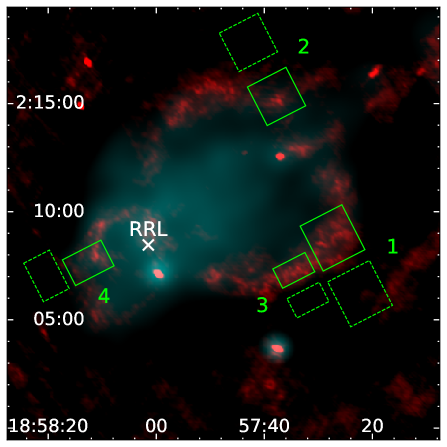
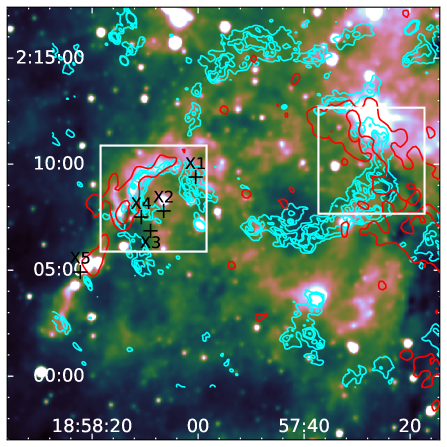
Figure 1: Colored images of the SNR-HIIR complex G35.6$-$0.4 in equatorial coordinate system. Left: The 610 MHz and 1.4 GHz data are represented in red and cyan, respectively. The green solid and dashed boxes mark the source and background regions for studying the HI absorption, respectively. The white cross represents the RRLs found by Lockman (1989). Right: WISE 12$\,\mu\rm m$ image superposed with GMRT 610 MHz contours (cyan) in levels of 0.44, 0.66, and 0.88$\,{\rm mJy\,beam^{-1}}$ (Paredes et al., 2014) and Nobeyama ¹²CO $(J=1-0)$ contours (red) in levels of 15 and 30$\,{\rm K}\,\,{\rm km}\,{\rm s}^{-1}$ in the velocity range of $+53-+57\,{\rm km}\,{\rm s}^{-1}$. The two white boxes represent the regions used to plot the grids of CO spectra. The black crosses are the X-ray sources found by Paredes et al. (2014).

2 Observations and Data

2.1 Fermi-LAT Observational data

In this study, we analyze more than 12 years (from 2008-08-04 15:43:36 (UTC) to 2020-11-30 05:38:25 (UTC)) of Fermi-LAT Pass 8 SOURCE class (evclass=128, evtype=3) data in the energy range 0.2-500 GeV using the python package Fermipy (v1.0.1) (Wood et al., 2017). The corresponding instrument respond functions (IRFs) are “P8R3_SOURCE_V3_v1”. The region of interest (ROI) is a $15\arcdeg\times 15\arcdeg$ square centered at the position of SNR G35.6$-$0.4 (RA = 284.479$\arcdeg$, Dec = 2.217$\arcdeg$). We only select the events within a maximum zenith angle of 90$\arcdeg$ to filter out the background $\gamma$-rays from the Earth’s limb and apply the recommended filter string “($\rm DATA\_QUAL>0)\&\&(LAT\_CONFIG==1$)” to choose the good time intervals. The Galactic diffuse emission (gll_iem_v07.fits) and isotropic emission (iso_P8R3_SOURCE_V3_v1.txt), as well as all the sources listed in the LAT 10-year Source Catalog (4FGL-DR2, Abdollahi et al., 2020) within a radius of $25\arcdeg$ from the ROI center, are included for background modeling, namely the baseline model.

2.2 CO observations and archival data

The observations of ¹²CO $J$=1–0 (at 115.271 GHz) and ¹³CO $J$=1–0 (at 110.201 GHz) were made during 2013 April-May with the 13.7-m millimeter-wavelength telescope of the Purple Mountain Observatory at Delingha (PMOD), China. The total bandwidth of the fast Fourier transform spectrometer of PMOD is 1 GHz and the half-power beamwidth is about 50^′′ for the two lines. The typical RMS noise level is about 0.5 K for ¹²CO ($J$=1–0) at the velocity resolution of 0.16 $\,{\rm km}\,{\rm s}^{-1}$ and 0.3 K for ¹³CO ($J$=1–0) at 0.17 $\,{\rm km}\,{\rm s}^{-1}$.

We also use the archival ¹²CO data of the FOREST Unbiased Galactic plane Imaging survey with the Nobeyama 45-m telescope (FUGIN, Umemoto et al., 2017) observation. The data have an angular resolution of $20^{\prime\prime}$ and an average RMS of 1.5 K at a velocity resolution of 0.65 $\,{\rm km}\,{\rm s}^{-1}$.

2.3 Other data

We also retrieve the Very Large Array (VLA) radio continuum image at 1.4 GHz and HI data from the HI/OH/recombination line survey (THOR) project (Beuther et al., 2016; Wang et al., 2020). The data have a spatial resolution of $25^{\prime\prime}$ and a velocity resolution of 1.5 $\,{\rm km}\,{\rm s}^{-1}$.

3 Data analysis and Results

3.1 Fermi-LAT Data Analysis

3.1.1 Spatial Analysis

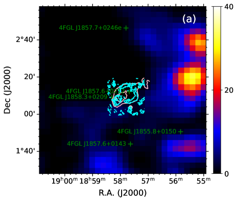
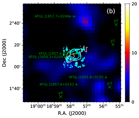
Figure 2: TS maps of a $1.5\arcdeg\times 1.5^{\circ}$ region centered at SNR G35.6$-$0.4 in the energy range of 0.2–500 GeV. Image is smoothed by the pixel size of $0.05^{\circ}$. The pink and cyan contours represent the SNR-HIIR complex G35.6$-$0.4 in 1.4 GHz (Stil et al., 2006) and 610 MHz (Paredes et al., 2014), respectively. Left: baseline model; Right: four point sources p1–p4 with positions listed in Table 3.1.1 are included in the source model.

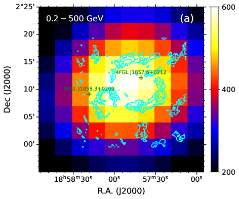
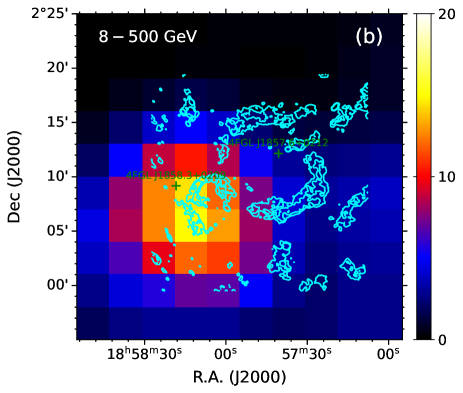
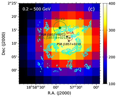
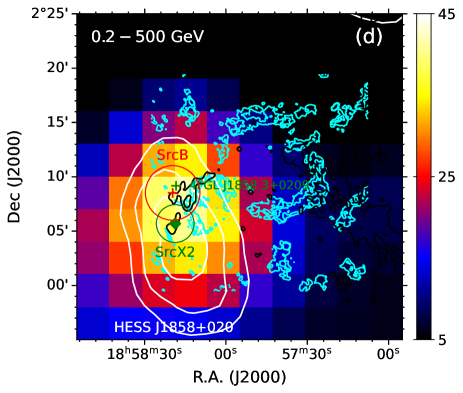
Figure 3: Same as Figure 2 but in a $0.5\arcdeg\times 0.5^{\circ}$ region. (a) 4FGL J1857.6+0212 and 4FGL J1858.3+0209 are excluded from the source model in the energy range 0.2–500 GeV. (b) Same as (a) but in 8–500 GeV. (c) SrcA (4FGL J1857.6+0212) is excluded from the source model. Two pulsars are also marked with the black crosses. (d) Same as (c) but for SrcB (4FGL J1858.3+0209). The white and black contours show the TeV source HESS J1858+020 (H. E. S. S. Collaboration et al., 2018) with 5, 6, and 7$\sigma$ significance and the Nobeyama ${}^{12}\mathrm{CO}$ ($J$=1$-$0) emission with levels [15, 30] K $\,{\rm km}\,{\rm s}^{-1}$ in the velocity range of +53 – +57 $\,{\rm km}\,{\rm s}^{-1}$, respectively. For (c) and (d), the green diamonds show the best-fit positions obtained by Cui et al. (2021) with 1$\sigma$ error shown in black circles. The refitted positions with 1$\sigma$ uncertainty in this study are marked by the red plus and circle. The original positions listed in 4FGL-DR2 are displayed in the green plus.

We note that there are two 4FGL-DR2 catalog sources 4FGL J1857.6+0212 and 4FGL J1858.3+0209 toward the SNR-HIIR complex G35.6$-$0.4 region. They are first treated as backgrounds to check the residual emission around our target. We use fit method to refit the spectral parameters of the sources within $3^{\circ}$ from the ROI center with the significance above $4\sigma$ and the normalization parameters of the two diffuse background components. Then, we fix all parameters except for the normalization of the Galactic diffuse emission to their best-fit values and generate the residual test-statistic (TS) map which is shown in the left panel of Figure 2. Here, the TS value is defined as TS = 2log($L_{1}/L_{0}$), in which $L_{0}$ is the maximum likelihood of the null hypothesis and $L_{1}$ the maximum likelihood with a putative source located in this pixel. As can be seen in Figure 2a, there is still strong residual emission to the west of the SNR-HIIR complex. We thus add three point sources with simple powerlaw spectra located at the peak pixels with TS $>$ 20, the positions of which are listed in Table 3.1.1, to model the residuals and repeat the above procedures. After this, we find that there is still some excess to the south of the complex. We then try adding this access as the fourth point source with powerlaw spectrum. Compared to the 3-point-source model, the likelihood of 4-point-source model can be increased by about 15, resulting in $\mathrm{TS_{model}}$=2log$(L_{\rm 4ps}/L_{\rm 3ps})\approx 30$. So we use the 4 point sources to model the residual emission. Finally, the background-subtracted TS map is displayed in Figure 2b.

Next, we study the $\gamma$-ray morphology toward SNR-HIIR complex G35.6$-$0.4 in detail. After excluding the 4FGL-DR2 catalog sources 4FGL J1857.6+0212 and 4FGL J1858.3+0209 from the source model, the TS maps in 0.2–500 GeV and 8–500 GeV are shown in Figures 3a and 3b, respectively. As can be seen, there is little emission above 8 GeV in the SNR region (represented by the bigger radio contours), while the emission at such energies concentrates on the HII region (represented by the smaller radio contours), suggesting that there are likely two sources. Meanwhile, we use the likelihood ratio to test three spatial models: one point source, one uniform disk, and two point sources. The model with the largest likelihood value will be preferred. To do so, we first use one point source with a LogParabola (LogP) spectrum, and then explore its best-fit position and extension to obtain the likelihood values of $L_{\rm 1ps}$ for the one-point-source model and $L_{\rm disk}$ for the uniform-disk model. For the two-point-source model, we use the templates of 4FGL J1857.6+0212 and 4FGL J1858.3+0209 and refit their best-fit positions, resulting in SrcA (RA = $284.418\arcdeg$, Dec = $2.192\arcdeg$, 1$\sigma$ error = $0.016\arcdeg$) and SrcB (RA = $284.582\arcdeg$, Dec = $2.142\arcdeg$, 1$\sigma$ error = $0.042\arcdeg$) for 4FGL J1857.6+0212 and 4FGL J1858.3+0209, respectively. The extension of the two sources are also explored, giving ${\rm TS}_{\rm ext}=2.4$ and 4.0 for SrcA and SrcB, respectively. Finally, according to the likelihood values for the three spatial models, we obtain $\mathrm{TS}_{\rm disk}=2\mathrm{log}(L_{\rm disk}/L_{\rm 1ps})=13$ and ${\rm TS}_{\rm 2ps}=30$ for the uniform-disk and two-point-source models, respectively. Considering the TS distribution in the different energy ranges and the likelihood ratio test for the three spatial models, two-point-source model for the SNR-HIIR complex G35.6$-$0.4 is preferred and used in the following analysis. The TS values of SrcA and SrcB in the two-point-source model is fitted to be 761.2 and 55.3, corresponding to the significance of 27.1$\sigma$ and 6.7$\sigma$, respectively.

In Figure 3, the TS maps for SrcA and SrcB are also presented in the second row panels. Our best-fit positions with 1$\sigma$ uncertainty are displayed with the red pluses and circles, respectively. For comparison, the 4FGL-DR2 positions and the best-fit ones in Cui et al. (2021) are shown with green pluses and green diamonds, respectively. As can be seen, the new best-fit positions for the both sources are very close to their original ones listed in the catalog, but are different from those in Cui et al. (2021), in particular for SrcA. To check this difference, we fit the positions by just using 5–500 GeV data and obtain similar results to those of our above treatment in 0.2–500 GeV, ruling out the effect of different energy range used in the two studies. Further, we repeat the analysis in Cui et al. (2021) by replacing the IRFs “P8R3_SOURCE_V3_v1” with “P8R3_SOURCE_V2_v1” and using 8-yr catalog for the background, and reproduce the results in Cui et al. (2021). Thus, the discrepancy in the best-fit position for SrcA is verified to be caused by using different IRFs and catalogs.

Table 1: Locations and TS value of the peak pixels in the left panel of Figure 2

Name	R.A.(J2000)	Dec (J2000)	TS
p1	283.850	2.345	41.5
p2	283.800	2.650	39.1
p3	283.900	1.695	23.5
p4	284.653	1.549	16.5

3.1.2 Spectral Analysis

In the 4FGL-DR2 catalog, the spectral types of SrcA and SrcB are LogP and PowerLaw (PL), respectively. To study the spectral properties of the both sources in the whole energy range of 0.2–500 GeV, other spectral types including ExpCutoffPowerLaw (ECPL) and BrokenPowerLaw (BPL) will also be explored. We first change the spectral type of SrcA to PL, ECPL, and BPL, respectively, to find the best spectral type. At the same time, the spectral type of SrcB remains to be PL. After this, we keep the best choice for SrcA and change the spectral type of SrcB to LogP, ECPL, and BPL, respectively, to find the best spectral formula for SrcB. The formulae of these spectra are listed in Table 3.1.2. The spectral type is favored if it has the largest TS value defined as $\mathrm{TS_{model}}=-2\mathrm{log}(L_{\mathrm{PL}}/L_{\mathrm{model}})$. As shown in Table 3.1.2, a LogP spectrum is preferred for SrcA. But for SrcB, there is no obvious difference for the four spectral types and the simplest PL form is adopted. Finally, we obtain the fluxes in 0.2–500 GeV as $4.2\times 10^{-11}\ {\rm erg\ \,{\rm cm}^{-2}\ s^{-1}}$ (with $\Gamma=2.66\pm 0.07$ and $\beta=0.44\pm 0.06$ for $E_{0}$=1.57 GeV) and $1.1\times 10^{-11}\ {\rm erg\ \,{\rm cm}^{-2}\ s^{-1}}$ (with $\Gamma=2.19\pm 0.09$) for SrcA and SrcB, respectively.

The spectral energy distributions (SEDs) within 0.2–500 GeV of SrcA and SrcB are generated by using the maximum likelihood analysis in seven logarithmically spaced energy bins. During the fitting process, the free parameters only include the normalization parameters of the sources with the significance $4\sigma$ within $5^{\circ}$ from the ROI center as well as the Galactic and isotropic diffuse background components, while all the other parameters are fixed to their best-fit values from the above analysis in the whole energy (0.2–500 GeV) range. In the energy bins where the TS value of SrcA or SrcB is smaller than 4, we calculate the 95%-confidence-level upper limit of its flux. The results are displayed in Figure 9.

Table 2: Formulae for $\gamma$-ray spectra

Name	Formula	Free parameters
PL	$dN/dE=N_{0}(E/E_{0})^{-\Gamma}$	$N_{0},\Gamma$
ECPL	$dN/dE=N_{0}(E/E_{0})^{-\Gamma}\mathrm{exp}(-E/E_{\mathrm{cut}})$	$N_{0},\Gamma,E_{\mathrm{cut}}$
LogP	$dN/dE=N_{0}(E/E_{0})^{-\Gamma-\beta\mathrm{log}(E/E_{0})}$	$N_{0},\Gamma,\beta$
BPL	$dN/dE=N_{0}\cases{(E/E_{\mathrm{b}})^{-\Gamma_{1}},E\leq E_{\mathrm{b}}\\ (E/E_{\mathrm{b}})^{-\Gamma_{2}},E\geq E_{\mathrm{b}}}$	$N_{0},E_{\mathrm{b}},\Gamma_{1},\Gamma_{2}$

Table 3: The Likelihood Test Results ($\mathrm{TS_{model}}$) from the Spectral Analysis of SrcA and SrcB

	$\mathrm{TS_{PL}}$	$\mathrm{TS_{ECPL}}$	$\mathrm{TS_{LogP}}$	$\mathrm{TS_{BPL}}$
SrcA	0	70.1	88.9	76.7
SrcB	0	0.1	1.7	2.3

3.2 Molecular environments

The ¹²CO spectra toward SNR G35.6$-$0.4 show multiple line components from $+6\,{\rm km}\,{\rm s}^{-1}$ to $+100\,{\rm km}\,{\rm s}^{-1}$. At $V_{\scriptscriptstyle\rm LSR}$ lower than $\sim+40\,{\rm km}\,{\rm s}^{-1}$ or higher than $\sim+70\,{\rm km}\,{\rm s}^{-1}$, little spatial correspondence between the MCs and the SNR can be found from the CO emission. Figure 4 shows the spatial distribution of the Nobeyama ¹²CO emission in velocity range $\sim+47$ to $+58\,{\rm km}\,{\rm s}^{-1}$, with velocity intervals of $0.65\,{\rm km}\,{\rm s}^{-1}$. The molecular gas in this velocity range seems to generally have a spatial correspondence with the western edge of SNR G35.6$-$0.4. In particular, a bright, clearcut molecular filament nicely follows the western shell of SNR G35.6$-$0.4 at $V_{\scriptscriptstyle\rm LSR}\sim+50\,{\rm km}\,{\rm s}^{-1}$. Notably, the peak ¹²CO main-beam temperature of the filament is about 20 K, which is noticeably higher than the typical temperature of $\sim 10$ K in interstellar MCs.

To investigate whether the molecular gas at the western edge of SNR G35.6$-$0.4 in the velocity range is perturbed by the shock of the SNR shock, we inspect the CO line grid toward this region. As shown in a grid of both ¹²CO ($J$=1–0) and ¹³CO($J$=1–0) spectra covering the western edge of the SNR at $V_{\scriptscriptstyle\rm LSR}\sim+50$ – $+70\,{\rm km}\,{\rm s}^{-1}$ (see Figure 5), the red wings of the ¹²CO lines, which peak at around $+57\,{\rm km}\,{\rm s}^{-1}$, seem to be asymmetrically broadened from about $+59$ to $+64\,{\rm km}\,{\rm s}^{-1}$, and these features are only presented within the boundary of the SNR. Figure 6 shows the averaged CO line profiles of a few pixels at the western edge of the SNR (regions ‘A’ and ‘B’, as marked in Figure 5). In these regions, at $V_{\scriptscriptstyle\rm LSR}\sim+59$ – $+64\,{\rm km}\,{\rm s}^{-1}$, there are non-negligible ¹²CO intensities while there is little ¹³CO emission. Because the ¹³CO is usually optically thin and yielded in quiescent, intrinsically high-column-density molecular material, an asymmetrical ¹²CO-line profile without a similar ¹³CO counterpart could be a kinematic signature of shock perturbation of the molecular gas. Therefore, the broadened ¹²CO red wings indicate that the MCs in this velocity range are probably perturbed by SNR G35.6$-$0.4.

Toward HIIR G35.6$-$0.5, there some noteworthy features at similar LSR velocities. First, there is a thin ¹²CO molecular arc at $V_{\scriptscriptstyle\rm LSR}\sim+55$–$+57~{}\,{\rm km}\,{\rm s}^{-1}$, which corresponds to the “northern clump” described in Paron & Giacani (2010) and delineates the semi-ring of the HIIR, consistent with the previous ¹³CO studies (Paron & Giacani, 2010; Paron et al., 2011). The peak main-beam temperature at the molecular arc is $T_{\rm mb}\sim 22~{}\,{\rm K}$, which is also noticeably higher than the typical temperature of $\sim 10$ K in quiescent interstellar MCs. Secondly, the wings of both the ¹²CO ($J$=1–0) and the ¹³CO ($J$=1–0) lines at a few positions along the molecular arc seem to be slightly asymmetric (see Figure 7). Actually, the asymmetry of the ¹³CO lines have been noted in Paron & Giacani (2010). The morphological agreement, together with the relatively high temperature and the asymmetric CO line profiles, supports the association between the molecular arc and the HII region. Thirdly, a cloudlet at $+52$ – $+55\,{\rm km}\,{\rm s}^{-1}$, corresponding to the “southern” (in the Galactic coordinated system) clump in Paron & Giacani (2010), is present outside the southeastern edge of the HIIR (see Figure 4) and is spatially close to the centroid of HESS J1858+020 (see Figure 3d). Especially, the peak of the main-beam temperature of the cloudlet ($\gtrsim 20$ K) is also significantly high.

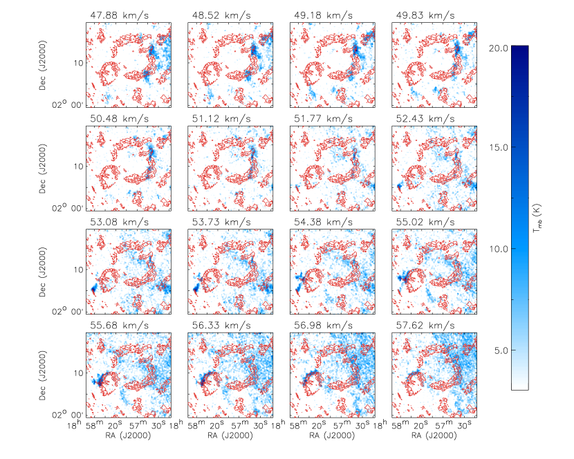
Figure 4: Channel map of the main-beam temperature of Nobeyama ¹²CO $J$=1–0 emission with a step of 0.65 $\,{\rm km}\,{\rm s}^{-1}$, overlaid with contours of GMRT 610 MHz radio emission.

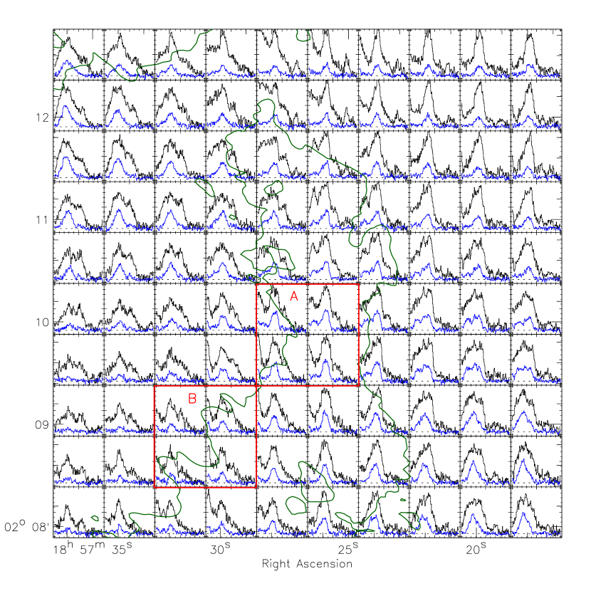
Figure 5: Grid of PMOD ¹²CO (black) and ¹³CO (blue) line profiles in the velocity range of $+50$ – $+70$ $\,{\rm km}\,{\rm s}^{-1}$for the region delineated by the right white box marked in Figure 1 in the SNR region. The GMRT 610 MHz contour of 0.44 mJy beam^-1 is shown in green. The size of each pixel is $30^{\prime\prime}\times 30^{\prime\prime}$. The averaged spectra from regions “A” and “B” are shown in Figure 6.

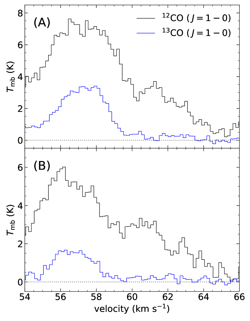
Figure 6: PMOD CO spectra in the $+54$ – $+66$ $\,{\rm km}\,{\rm s}^{-1}$interval for the two regions marked in Figure 5. The black and blue lines are for the ¹²CO ($J=1-0$) and ¹³CO ($J=1-0$), respectively.

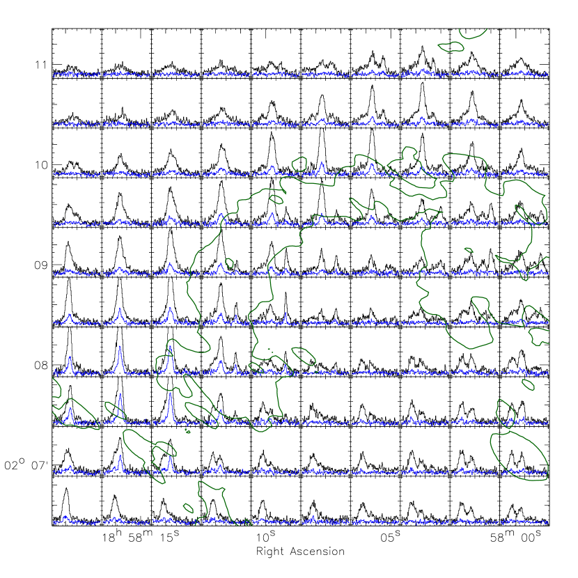
Figure 7: Same as Figure 5 but for HIIR in the velocity range of $+48$ – $+68$ $\,{\rm km}\,{\rm s}^{-1}$.

4 Discussion

4.1 Distances to the HIIR and SNR

Based on the association with the +55 – +56$\,{\rm km}\,{\rm s}^{-1}$ MCs suggested by Paron & Giacani (2010), the distance to SNR-HIIR complex G35.6$-$0.4 was constrained as $3.6\pm 0.4$ kpc by the HI absorption feature (Zhu et al., 2013). The HI absorption spectra abstracted from the radio continuum brightness peak region (very close to the position of RRLs) show the maximum absorption velocity around +61 $\,{\rm km}\,{\rm s}^{-1}$, supporting the near distance. However, the radio image of SNR G35.6$-$0.4 presented in previous works (e.g., Green, 2009) was later resolved into two circular structures by GMRT (Paredes et al., 2014). Although these two structures are projectively connected with each other, they may be at different distances. Thus the HI absorption spectra in Zhu et al. (2013) abstracted from the overlapped region of the two circles maybe only give constraint on the distance to one of them. To separately give constraint on the distances to the two structures, we examine HI absorption by selecting other regions marked in green boxes in Figure 1 and avoiding the overlapped region of the two circles.

The systemic velocity of the eastern HIIR has been well measured as $\sim+56~{}\,{\rm km}\,{\rm s}^{-1}$ according to the RRLs (Lockman, 1989) and CO observations (Paron & Giacani, 2010, and also this study). Assuming a flat Galactic rotation curve and adopting $R_{0}=8.34\,{\rm kpc}$ and $V_{0}=240\,{\rm km}\,{\rm s}^{-1}$ (Reid et al., 2014), this velocity corresponds to both a near distance $3.4\pm 0.4$ kpc and a far distance $10.2\pm 0.5$ kpc (Wenger et al., 2018; Reid et al., 2014), while the latter distance can be ruled out by HI absorption analysis. We follow the methods of Tian & Leahy (2008) and plot the HI absorption spectra, where the HI and continuum data are taken from the THOR and VLA data. The HI absorption is calculated as $e^{\tau}=1-(T_{\rm off}^{\rm HI}-T_{\rm on}^{\rm HI})/(T_{\rm s}^{c}-T_{\rm bg}^{c})$, where $T_{\rm on}^{\rm HI}$ and $T_{\rm off}^{\rm HI}$ are HI temperatures at the source and background regions, and $T_{\rm s}^{c}$ and $T_{\rm bg}^{c}$ are the radio continuum brightness temperatures at the source and background regions, respectively. For the HIIR, the HI absorption spectrum is obtained from the region with label ‘4’ in Figure 1 and is displayed in the fourth panel of Figure 8, showing that the maximum absorption velocity is $\sim+60\,{\rm km}\,{\rm s}^{-1}$. This absorption feature is consistent with the results in Zhu et al. (2013) and supports the near distance.

SNR G35.6$-$0.4 was presumed to be associated with its eastern (in the equatorial coordinate system) HII region, as an MC revealed from the ¹³CO emission is projected at the eastern border of the SNR (Paron & Giacani, 2010). Our ¹²CO analysis has instead shown a strong morphological agreement between the SNR’s western boundary and a warm molecular filament at $V_{\scriptscriptstyle\rm LSR}\sim+50~{}\,{\rm km}\,{\rm s}^{-1}$. The velocity corresponds to both a near distance $3.0\pm 0.4$ kpc and a far distance $10.5\pm 0.4$ kpc, which will below be discriminated with an HI absorption analysis.

We inspect HI absorption toward the SNR, which has not been examined in previous literature, so as to put an additional constraint on the distance to it. the HI and continuum data are taken from the THOR VLA data. The HI absorption is calculated as $e^{\tau}=1-(T_{\rm off}^{\rm HI}-T_{\rm on}^{\rm HI})/(T_{\rm s}^{c}-T_{\rm bg}^{c})$, where $T_{\rm on}^{\rm HI}$ and $T_{\rm off}^{\rm HI}$ are HI temperatures at the source and background regions, and $T_{\rm s}^{c}$ and $T_{\rm bg}^{c}$ are the radio continuum brightness temperatures at the source and background regions, respectively. The selected source and background regions are displayed in Figure 1 with labels ‘1’, ‘2’, and ‘3’. Figure 8 shows significant HI absorption in all of the three regions of the SNR at $V_{\rm LSR}\sim+80$ $\,{\rm km}\,{\rm s}^{-1}$, which corresponds to a distance of $4.7\pm 0.7$ kpc or $8.9\pm 0.8$ kpc. Therefore, the SNR distance should be larger than $4.7\pm 0.7$ kpc so as to explain the existence of the HI absorption at $\sim+80~{}\,{\rm km}\,{\rm s}^{-1}$. Therefore, the SNR is located at the far distance $10.5\pm 0.4\,{\rm kpc}$, behind the tangent point toward the same line-of-sight (at $\sim 6.8\,{\rm kpc}$). Thus, SNR G35.6$-$0.4 and HIIR G35.6$-0.5$ are irrelevant to each other, given the different kinematic distances to them ($\sim 10.5\,{\rm kpc}$ and $3.4\,{\rm kpc}$, respectively).

By taking the two distances, the masses/densities of the MCs associated with SNR G35.6$-$0.5 and HIIR G35.6$-$0.5 are estimated to be about $9\times 10^{3}\,M_{\odot}$/$70\,{\rm cm}^{-3}$ and $1.3\times 10^{3}\,M_{\odot}$/$290\,{\rm cm}^{-3}$, respectively.

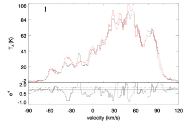
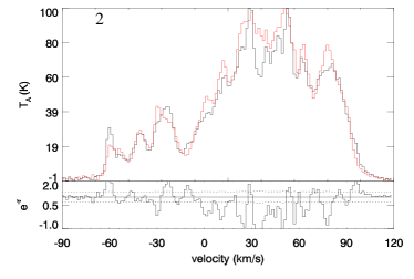
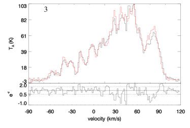
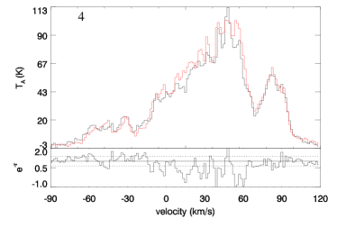
Figure 8: HI spectra (upper panels; red: background; black: source) and HI absorption spectra (lower panels) in three regions toward the SNR region. The numbers in the left-top corner of each panel represent the regions 1, 2, 3, and 4 labeled in Figure 1. The horizontal dotted lines in the lower panels indicate the $\pm 3\sigma$ uncertainty level of the HI absorption spectra.

4.2 Origin of gamma-rays

4.2.1 SNR G35.6$-$0.4

As shown in Figure 3c, SrcA is located within the shell of SNR G35.6$-$0.4 and is projectively close to two pulsars PSR J1857+0212 and PSR J1857+0210. We first discuss the possibility of pulsar’s origin. According to the dispersion measures, PSR J1857+0212 and PSR J1857+0210 are at distances 7.98 kpc (Han et al., 2006) and 15.4 kpc (Morris et al., 2002), respectively. But the distances are revised to 6.0 kpc and 7.3 kpc in the ATNF pulsar catalog (Manchester et al., 2005), respectively, based on the new electron-density model developed by Yao et al. (2017). Taking 6.0 kpc (the smaller one) for example, SrcA would have a luminosity of $\sim 2\times 10^{35}d_{\rm 6kpc}^{-2}\ {\rm erg\ s^{-1}}$ in the energy range 0.2–500 GeV, where $d_{\rm 6kpc}$is distance in unit of 6 kpc, which is significantly higher than the spin-down luminosity of $2.2\times 10^{34}\ {\rm erg\ s^{-1}}$ for PSR J1857+0212 (Han et al., 2006; Manchester et al., 2005) and $2.2\times 10^{33}\ {\rm erg\ s^{-1}}$ for PSR J1857+0212 (Morris et al., 2002; Manchester et al., 2005). Thus the pulsar’s origin for SrcA can be ruled out unless the true distance is smaller than 2 kpc for PSR J1857+0212 and 0.7 kpc for PSR J1857+0210.

SNR G35.6$-$0.4 may be responsible for the $\gamma$-ray emission of SrcA, and we provide estimates for the emission in cases of hadronic and leptonic interaction separately. We simply assume that the particles accelerated in the SNR have a power-law form with a high-energy cutoff:

$$dN_{i}/dE=A_{i}(E/E_{0})^{-\alpha_{i}}\mathrm{exp}(-E/E_{i,c})$$ (1)

where, $i=e,p$, $\alpha_{i}$ and $E_{i,c}$ are the power-law index and high-energy cutoff, respectively. The normalization $A_{i}$ is determined by the total energy ($W_{i}$) in particles with energy above 1 GeV. Since the SNR is very likely to be associated with the $\sim+50\,{\rm km}\,{\rm s}^{-1}$ MC at a distance of $\sim 10.5$ kpc as revealed above, the $\gamma$-ray emission arising from the SNR-accelerated particles’ hadronic interaction is first considered. In such a hadronic scenario, SrcA’s spectrum can be well fit (as shown in the left panel of Figure 7) and we obtain $\alpha_{p}\approx 3.0$ and $n_{0}W_{p}\approx 8\times 10^{51}\ {\rm erg\ cm^{-3}}$, where $n_{0}$ is the number density of the target gas for proton-proton hadronic interaction. The cutoff energy can not be constrained by the current data and is fixed as 3 PeV in our calculation. With the mass of $9\times 10^{3}\,M_{\odot}$ and an average atomic hydrogen density $n_{0}\sim 140\ {\rm cm^{-3}}$ for the $\sim+50\,{\rm km}\,{\rm s}^{-1}$ filamentary molecular gas, the energy budget in protons $W_{p}$ is about $6\times 10^{49}$ erg, which is acceptable and reasonable for the SNR scenario. The somewhat large index may be attributed to the strong ion-neutral collisions (Malkov et al., 2011) or the escaped process (e.g., Aharonian & Atoyan, 1996; Li & Chen, 2012). In addition, the luminosity of SrcA in 1–100 GeV is $2\times 10^{36}\ {\rm erg\ s^{-1}}$, which is consistent with the known $\gamma$-ray-bright interacting SNRs (Liu et al., 2015; Acero et al., 2016). Thus the hadronic scenario in which the energetic protons are from SNR G35.6$-$0.4 is a plausible explanation for SrcA.

For the leptonic case in which $\gamma$-rays are produced via the inverse Compton (IC) process, due to the lack of constraint on the index by the GeV data, we fix $\alpha_{e}=2.0$ based on the radio index $\alpha_{r}=0.47$ (Green, 2009). To explain the data (see the model curve in orange in the left panel of Figure 9), $E_{e,c}\approx 80$ GeV and $W_{e}\approx 7\times 10^{50}$ erg are obtained when the seed photons include the IR emission with a temperature of 35 K and an energy density of 0.6 ${\rm eV\ cm^{-3}}$ estimated from the interstellar radiation field (ISRF) model (Porter et al., 2006; Shibata et al., 2011) and the cosmic microwave background. Considering the large amount of energy in electrons which is comparable to the canonical supernova explosion energy, the leptonic process seems not proper to explain the $\gamma$-ray emission of SrcA unless there is unusually strong IR emission.

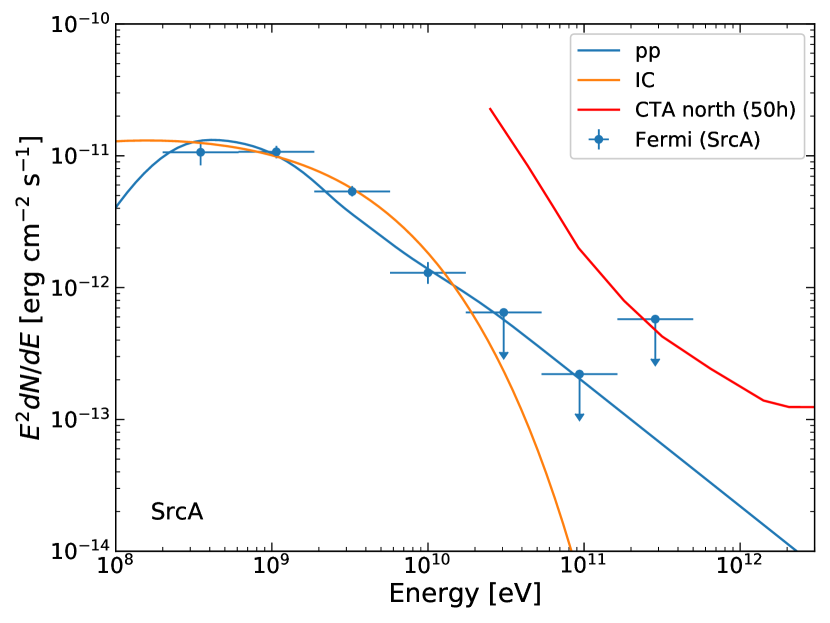
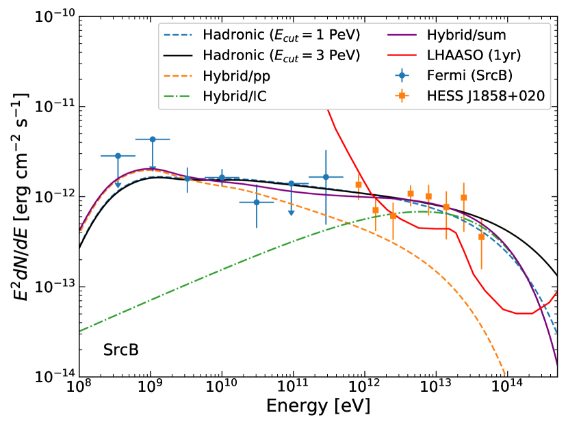
Figure 9: SED of SrcA (SNR G35.6$-$0.4) and SrcB (HII region G35.6$-$0.5 and HESS J1858+020). The TeV data of HESS J1858+020 are taken from Aharonian et al. (2008). The sensitivity of CTA north (50h; Cherenkov Telescope Array Consortium et al., 2019) and LHAASO (1yr; di Sciascio & Lhaaso Collaboration, 2016) are also displayed in the left and right panel, respectively.

4.2.2 HIIR G35.6$-$0.5 and HESS J1858+020

As shown in Figure 3d, the GeV source SrcB is spatially coincident with the unidentified TeV source HESS J1858+020. Moreover, the GeV spectrum of SrcB can be well connected with the TeV spectrum of HESS J1858+020 by a simple power-law function with an index of $\sim$2.2 (see the right panel in Figure 9). Thus, SrcB is very likely the GeV counterpart of TeV source HESS J1858+020. Meanwhile, both sources are spatially coincident with the MCs at a velocity around the $\sim$ +53–+57 $\,{\rm km}\,{\rm s}^{-1}$which have a mass of $1.3\times 10^{3}\,M_{\odot}$ and an average atomic hydrogen number density of $600\ {\rm cm^{-3}}$. As suggested in Paron & Giacani (2010) and this work (§3.2), this molecular arc is likely associated with HIIR G35.6$-$0.5. Both the association with MCs and the soft GeV-TeV spectra (index $>$2) suggest the GeV-TeV $\gamma$-ray emissions likely have a hadronic origin. One possible scenario for SrcB and HESS J1858+020 is that the energetic protons accelerated in HIIR G35.6$-$0.5 bombard the MC to produce the hadronic $\gamma$-ray emission. By adopting a distance of 3.4 kpc, $\alpha_{p}\approx 2.15$ and $W_{p}\approx 1.7\times 10^{47}$ erg are obtained. To explain the TeV data which look without an obvious cutoff, the cutoff energy of protons $E_{p,c}$ should reach the PeV energy (see the right panel of Figure 9). This implies that there may be a potential PeV accelerator in HIIR G35.6$-$0.5. This can be tested by the LHAASO experiment in the future. As one of the PeVatron candidates, the lower limit of the proton cutoff energy $\sim$30 TeV for HESS J1858+020 is obtained by only using the TeV data (Spengler, 2020). In fact, the index and the cutoff energy are strongly degenerated. We note that the index constrained in Spengler (2020) for this source is obviously smaller than 2.0. With the help of the GeV data, the index is fitted as $\sim$2.2 in this study, resulting in a larger cutoff energy.

HIIRs, varies from $\sim$0.1 pc to hundred pc in size, are generally related to the active star formations and are considered as particle accelerators. It has been proposed that particles can be accelerated by the colliding winds of binaries (e.g., Eichler & Usov, 1993) and/or the young massive clusters (Aharonian et al., 2019) which are the ionising sources of HIIRs. This is supported by the TeV $\gamma$-ray observations towards $\eta$ Car (H. E. S. S. Collaboration et al., 2020) for the colliding winds and the Cygnus region (Aliu et al., 2014; Bartoli et al., 2014; Amenomori et al., 2021; Abeysekara et al., 2021) for the massive star clusters. In HIIR G35.6$-$0.5, although there are not massive stars detected as yet, Paron & Giacani (2010) found six young stellar object (YSO) candidates toward the molecular clump at $\sim$+53 $\,{\rm km}\,{\rm s}^{-1}$ (namely the southern clump in their paper) and concluded that there is an active star-formation region. Further observations found at least one evolved YSO (i.e., IRS1) is embedded in the clump, although no the signature of outflows was confirmed (Paron et al., 2011). By analyzing of the Chandra data, Paredes et al. (2014) found seven X-ray sources, and suggested that sources X1–4, almost projectively distributing on the shell of the HIIR (see the right panel of Figure 1), might be embedded protostars and that source X5, closing to the “southern” (in the Galactic coordinate system) clump, might be coincident with the star formation region. Thus, it could not be excluded that there may be some non-detected massive stars embedded in the MC.

Alternatively, we also consider the lepto-hadronic hybrid case in which the GeV emissions are from the hadronic process and the TeV $\gamma$-rays are generated by the IC process. We assume the electrons and protons have the same power-law index and high-energy cutoff. For the seed photons in the IC process, the IR component of ISRF is also included and is estimated as 35 K and 0.6 ${\rm eV\ cm^{-3}}$ by using the similar method for SrcA above. To explain the data (see the purple curve in the right panel of Figure 9), $\alpha_{e}=\alpha_{p}\approx 2.3$ and $E_{c,e}=E_{c,p}\approx 200$ TeV are obtained. Electrons will suffer the synchrotron radiation loss during the acceleration, giving a cooling-limited maximum energy $E_{max,cool}=35u_{3}/\sqrt{\eta_{g}B_{1}}$ TeV (e.g., Zirakashvili & Aharonian, 2007; Ohira et al., 2012), where $u_{3}$ is the shock velocity in unit of 1000 $\,{\rm km}\,{\rm s}^{-1}$, $\eta_{g}$ the gyrofactor, and $B_{1}$ the magnetic field strength in unit of 10 $\mu$G. For the wind velocity $u_{3}=1$ and the Bohm limit $\eta_{g}=1$, it requires $B<0.3\ \mu$G to boost the energy of electrons up to 200 TeV. This magnetic strength is as weak as an order of magnitude lower than the mean value for Galactic ISM, which means that it is hard to accelerate electrons to the 100 TeV band for the standard interstellar magnetic field. Thus, the hybrid model seems rather unlikely according to the fitted results.

5 Summary

In this study, we focus on the SNR-HIIR complex including SNR G35.6$-$0.4 and HIIR G35.6$-$0.5, which partially overlaps with the unidentified TeV source HESS J1858+020 with a hard spectrum. We reanalyze CO-line, HI, and Fermi-LAT GeV $\gamma$-ray emission data of this region. The main results are summarized as follows:

1. Based on the Nobeyama data, we found that a molecular arc at $\sim$+56 $\,{\rm km}\,{\rm s}^{-1}$ delineates the northern (in the equatorial coordinate system) shell of HIIR G35.6$-$0.5 and a molecular filament at $\sim$+50 $\,{\rm km}\,{\rm s}^{-1}$ nicely follows the western boundary of SNR G35.6$-$0.4. Such morphological agreements, together with the relatively high main-beam temperature and the asymmetric or broad CO line profiles, suggest that the two molecular structures are likely to be associated with the HIIR and the SNR, respectively.

2. The HI absorption features suggest that the SNR is located behind the tangent point, at a distance 10.5 kpc, and thus is not associated with the HIIR.

3. Performing the analysis of 12.3-year Fermi-LAT data, we found that there are two point sources (SrcA and SrcB) with significance of 27.1$\sigma$ and 6.7$\sigma$ in 0.2–500 GeV toward the SNR-HIIR complex, respectively. The two sources are spatially coincident with the SNR and the TeV source HESS J1858+020, respectively.

4. For SrcA, leptonic processes for the SNR scenario and the PSR scenario can be ruled out according to the energy budget. In the SNR-MC association scenario, the hadronic process can explain the spectrum with reasonable physical parameters.

5. For SrcB, its GeV-band spectrum can be smoothly connected with the TeV-band spectrum of HESS J1858+020 by a simple power-law function with an index of $\sim$2.2. In combination with the HIIR-MC association, it favors the hadronic origin. To explain the data, the cutoff energy of protons is the order of PeV. This indicates that there may be a potential PeV proton accelerator in HIIR G35.6$-$0.5, which needs to be tested with ultra-high energy observation, e.g., with LHAASO.

References

- Abdollahi et al. (2020) Abdollahi, S., Acero, F., Ackermann, M., et al. 2020, ApJS, 247, 33, doi: 10.3847/1538-4365/ab6bcb
- Abeysekara et al. (2021) Abeysekara, A. U., Albert, A., Alfaro, R., et al. 2021, Nature Astronomy, 5, 465, doi: 10.1038/s41550-021-01318-y
- Acero et al. (2016) Acero, F., Ackermann, M., Ajello, M., et al. 2016, ApJS, 224, 8, doi: 10.3847/0067-0049/224/1/8
- Aharonian et al. (2019) Aharonian, F., Yang, R., & de Oña Wilhelmi, E. 2019, Nature Astronomy, 3, 561, doi: 10.1038/s41550-019-0724-0
- Aharonian et al. (2008) Aharonian, F., Akhperjanian, A. G., Barres de Almeida, U., et al. 2008, A&A, 477, 353, doi: 10.1051/0004-6361:20078516
- Aharonian & Atoyan (1996) Aharonian, F. A., & Atoyan, A. M. 1996, A&A, 309, 917
- Aliu et al. (2014) Aliu, E., Aune, T., Behera, B., et al. 2014, ApJ, 783, 16, doi: 10.1088/0004-637X/783/1/16
- Altenhoff et al. (1970) Altenhoff, W. J., Downes, D., Goad, L., Maxwell, A., & Rinehart, R. 1970, A&AS, 1, 319
- Amenomori et al. (2021) Amenomori, M., Bao, Y. W., Bi, X. J., et al. 2021, Phys. Rev. Lett., 127, 031102, doi: 10.1103/PhysRevLett.127.031102
- Astropy Collaboration et al. (2013) Astropy Collaboration, Robitaille, T. P., Tollerud, E. J., et al. 2013, A&A, 558, A33, doi: 10.1051/0004-6361/201322068
- Astropy Collaboration et al. (2018) Astropy Collaboration, Price-Whelan, A. M., Sipőcz, B. M., et al. 2018, AJ, 156, 123, doi: 10.3847/1538-3881/aabc4f
- Bartoli et al. (2014) Bartoli, B., Bernardini, P., Bi, X. J., et al. 2014, ApJ, 790, 152, doi: 10.1088/0004-637X/790/2/152
- Beard & Kerr (1969) Beard, M., & Kerr, F. J. 1969, Australian Journal of Physics, 22, 121, doi: 10.1071/PH690121
- Beuther et al. (2016) Beuther, H., Bihr, S., Rugel, M., et al. 2016, A&A, 595, A32, doi: 10.1051/0004-6361/201629143
- Cherenkov Telescope Array Consortium et al. (2019) Cherenkov Telescope Array Consortium, Acharya, B. S., Agudo, I., et al. 2019, Science with the Cherenkov Telescope Array, doi: 10.1142/10986
- Cui et al. (2021) Cui, Y., Xin, Y., Liu, S., et al. 2021, A&A, 646, A114, doi: 10.1051/0004-6361/202039041
- di Sciascio & Lhaaso Collaboration (2016) di Sciascio, G., & Lhaaso Collaboration. 2016, Nuclear and Particle Physics Proceedings, 279-281, 166, doi: 10.1016/j.nuclphysbps.2016.10.024
- Eichler & Usov (1993) Eichler, D., & Usov, V. 1993, ApJ, 402, 271, doi: 10.1086/172130
- Green (2009) Green, D. A. 2009, MNRAS, 399, 177, doi: 10.1111/j.1365-2966.2009.14957.x
- H. E. S. S. Collaboration et al. (2018) H. E. S. S. Collaboration, Abdalla, H., Abramowski, A., et al. 2018, A&A, 612, A1, doi: 10.1051/0004-6361/201732098
- H. E. S. S. Collaboration et al. (2020) H. E. S. S. Collaboration, Abdalla, H., Adam, R., et al. 2020, A&A, 635, A167, doi: 10.1051/0004-6361/201936761
- Han et al. (2006) Han, J. L., Manchester, R. N., Lyne, A. G., Qiao, G. J., & van Straten, W. 2006, ApJ, 642, 868, doi: 10.1086/501444
- Li & Chen (2012) Li, H., & Chen, Y. 2012, MNRAS, 421, 935, doi: 10.1111/j.1365-2966.2012.20270.x
- Liu et al. (2015) Liu, B., Chen, Y., Zhang, X., et al. 2015, ApJ, 809, 102, doi: 10.1088/0004-637X/809/1/102
- Lockman (1989) Lockman, F. J. 1989, ApJS, 71, 469, doi: 10.1086/191383
- Malkov et al. (2011) Malkov, M. A., Diamond, P. H., & Sagdeev, R. Z. 2011, Nature Communications, 2, 194, doi: 10.1038/ncomms1195
- Manchester et al. (2005) Manchester, R. N., Hobbs, G. B., Teoh, A., & Hobbs, M. 2005, AJ, 129, 1993, doi: 10.1086/428488
- Morris et al. (2002) Morris, D. J., Hobbs, G., Lyne, A. G., et al. 2002, MNRAS, 335, 275, doi: 10.1046/j.1365-8711.2002.05551.x
- Ohira et al. (2012) Ohira, Y., Yamazaki, R., Kawanaka, N., & Ioka, K. 2012, MNRAS, 427, 91, doi: 10.1111/j.1365-2966.2012.21908.x
- Paredes et al. (2014) Paredes, J. M., Ishwara-Chandra, C. H., Bosch-Ramon, V., et al. 2014, A&A, 561, A56, doi: 10.1051/0004-6361/201322306
- Paron & Giacani (2010) Paron, S., & Giacani, E. 2010, A&A, 509, L4, doi: 10.1051/0004-6361/200913694
- Paron et al. (2011) Paron, S., Giacani, E., Rubio, M., & Dubner, G. 2011, A&A, 530, A25, doi: 10.1051/0004-6361/201016390
- Porter et al. (2006) Porter, T. A., Moskalenko, I. V., & Strong, A. W. 2006, ApJ, 648, L29, doi: 10.1086/507770
- Ranasinghe & Leahy (2018) Ranasinghe, S., & Leahy, D. A. 2018, AJ, 155, 204, doi: 10.3847/1538-3881/aab9be
- Reid et al. (2014) Reid, M. J., Menten, K. M., Brunthaler, A., et al. 2014, ApJ, 783, 130, doi: 10.1088/0004-637X/783/2/130
- Robitaille (2019) Robitaille, T. 2019, APLpy v2.0: The Astronomical Plotting Library in Python, doi: 10.5281/zenodo.2567476
- Robitaille & Bressert (2012) Robitaille, T., & Bressert, E. 2012, APLpy: Astronomical Plotting Library in Python. http://ascl.net/1208.017
- Shibata et al. (2011) Shibata, T., Ishikawa, T., & Sekiguchi, S. 2011, ApJ, 727, 38, doi: 10.1088/0004-637X/727/1/38
- Spengler (2020) Spengler, G. 2020, A&A, 633, A138, doi: 10.1051/0004-6361/201936632
- Stil et al. (2006) Stil, J. M., Taylor, A. R., Dickey, J. M., et al. 2006, AJ, 132, 1158, doi: 10.1086/505940
- Tian & Leahy (2008) Tian, W. W., & Leahy, D. A. 2008, ApJ, 677, 292, doi: 10.1086/529120
- Torres et al. (2011) Torres, D. F., Li, H., Chen, Y., et al. 2011, MNRAS, 417, 3072, doi: 10.1111/j.1365-2966.2011.19465.x
- Umemoto et al. (2017) Umemoto, T., Minamidani, T., Kuno, N., et al. 2017, PASJ, 69, 78, doi: 10.1093/pasj/psx061
- Wang et al. (2020) Wang, Y., Beuther, H., Rugel, M. R., et al. 2020, A&A, 634, A83, doi: 10.1051/0004-6361/201937095
- Wenger et al. (2018) Wenger, T. V., Balser, D. S., Anderson, L. D., & Bania, T. M. 2018, ApJ, 856, 52, doi: 10.3847/1538-4357/aaaec8
- Wood et al. (2017) Wood, M., Caputo, R., Charles, E., et al. 2017, in International Cosmic Ray Conference, Vol. 301, 35th International Cosmic Ray Conference (ICRC2017), 824. https://arxiv.org/abs/1707.09551
- Wright et al. (2010) Wright, E. L., Eisenhardt, P. R. M., Mainzer, A. K., et al. 2010, AJ, 140, 1868, doi: 10.1088/0004-6256/140/6/1868
- Yao et al. (2017) Yao, J. M., Manchester, R. N., & Wang, N. 2017, ApJ, 835, 29, doi: 10.3847/1538-4357/835/1/29
- Zabalza (2015) Zabalza, V. 2015, Proc. of International Cosmic Ray Conference 2015, 922
- Zhu et al. (2013) Zhu, H., Tian, W. W., Torres, D. F., Pedaletti, G., & Su, H. Q. 2013, ApJ, 775, 95, doi: 10.1088/0004-637X/775/2/95
- Zirakashvili & Aharonian (2007) Zirakashvili, V. N., & Aharonian, F. 2007, A&A, 465, 695, doi: 10.1051/0004-6361:20066494